Article

Robot Static Path Planning Method Based on Deterministic Annealing

1
School of Electronic and Information Engineering, Suzhou University of Science and Technology, Suzhou 215009, China
2
School of Automation Science and Electrical Engineering, Beihang University, Beijing 100191, China
*
Author to whom correspondence should be addressed.
These authors contributed equally to this work.
Machines 2022, 10(8), 600; https://doi.org/10.3390/machines10080600
Submission received: 28 May 2022 / Revised: 14 July 2022 / Accepted: 21 July 2022 / Published: 22 July 2022
(This article belongs to the Special Issue Advanced Control Theory with Applications in Intelligent Machines)

Abstract

:
Heuristic calculation is an essential method to solve optimisation problems. However, its vast computing requirements limit its real-time and online applications, especially in embedded systems with limited computing resources, such as mobile robots. This paper presents a robot path planning algorithm called DA-APF based on deterministic annealing. It is derived from the artificial potential field and can effectively solve the local minimum problem of the model established by the potential field method. The calculation performance of DA-APF is considerably improved by introducing temperature parameters to enhance the potential field function and by using annealing and tempering methods. Moreover, an optimal or near-optimal robot path planning scheme is given. A comprehensive case study is performed using heuristic methods, such as genetic algorithm and simulated annealing. Simulation results show that DA-APF performs well in various static path planning environments.

1. Introduction

Path planning is one of the essential links in autonomous mobile robot navigation. In accordance with a specific performance index, path planning aims to search for an optimal or nearly optimal collision-free path from the initial state to the target state. With the development of intelligent control technology and artificial intelligence algorithms, using a heuristic algorithm to solve the robot path planning problem has become one of the research hotspots in mobile robot control.
As a unique method to solve nonlinear problems, heuristic computing attracts extensive attention from researchers. It is a method to obtain and express information through calculation and simulate and realise intelligent behaviour. Given that complex practical problems require intelligent systems to combine knowledge, technologies and methods from different sources, these intelligent systems are expected have the same expertise as humans in specific fields, can adjust themselves to evolve learning ability in a changing environment, and can explain how to make decisions and take actions. The commonly used heuristic methods in robot path planning include genetic algorithm (GA) [1,2], simulated annealing algorithm (SA) [3,4], ant colony algorithm (ACO) [5,6] and particle swarm optimisation algorithm (PSO) [7,8].
However, the artificial potential field (APF) has some inherent flaws in path planning, and these include the absence of a feasible path in dense obstacle space, a path trajectory that goes beyond the equilibrium position, oscillating or repeatedly closed-loop in narrow space, and being trapped at the local minima before reaching the target. Two current solutions can be applied as follows: (1) redefining the potential function, removing or retaining only a small number of local minima (local minimum removal) and (2) avoiding obstacles (local minimum avoidance) or escaping from the local minima (local minimum escape) through intelligent search technology. To address the drawbacks of having an unreachable target and the tendency to fall easily into the local minima in the standard potential field, many scholars at home and abroad have proposed various improvement methods. Reference [9] proposed a fuzzy-based approach for path planning in addition to steering a robot out of local minima through a comparative analysis of some non-fuzzy approaches. In [10], two modified APF-based strategies for solving the dual-arm motion planning task in unknown environments were proposed. Both techniques use configuration sampling and subgoal selection to help APFs avoid local minima scenarios. Reference [11] introduced some modifications and improvements to APF to solve one-obstacle local minima, two-obstacle local minima, goal not-reachable with obstacles nearby and dynamic obstacles. Reference [12] proposed a method based on the combination of a modified APF algorithm with fuzzy logic, which was designed to overcome the problems of classical APF, especially the local minima, and enhanced the navigation in complex environments. Reference [13] proposed a method to avoid local minima. The method involves attracting equilibrium at the target point and repelling equilibriums in the obstacle centres and saddle points on the borders. The method was shown to be effective through a simulation of a two-variable integrator and subsequently applied to unicycle-like, wheeled mobile robots.
The main motivation of the current study is to propose a path planning algorithm based on deterministic annealing (DA) that is an improvement of the standard APF method and can be used for local and global path planning. This improvement does not employ the traditional branch-and-bound method and is thus relatively novel. The proposed algorithm, DA-APF, can prevent the robot from falling into the local minimum of the potential field. At the same time, due to the rapid convergence of DA, the algorithm demonstrates efficient computational performance. We introduce the DA-APF algorithm in detail and illustrate this method by examining the path planning of a model robot in a two-dimensional convex polygon or nonconvex polygon obstacle environment. In this work, the problem is simplified to make it suitable for the study of annealing parameters, but the method can be extended to more complex environments.
The remainder of this paper is organised as follows. The second section introduces the progress of latest research and conventional construction methods of APF. The third section presents the basic idea of DA and the DA-APF algorithm. The fourth section is the simulation part. These results prove the effectiveness of the proposed algorithm. The fifth section summarises this paper.

2. Artificial Potential Field

Khatib [14] was the first to apply the APF approach to path planning. This approach is suitable for real-time control of robots because of its clear physical meaning and simple mathematical description. Therefore, it has been widely used in path planning. The main reason is that the APF method provides a simple, efficient, reliable motion planner for realistic goals. The target generates attraction potential in this potential field, and the obstacle generates repulsion potential. Under the superposition of the two potential energies, the robot moves from a high potential field to a low potential field along the negative gradient direction of the whole potential field. Given that the target is designed as the global minimum with the lowest potential energy in the environment, theoretically, the robot’s motion will eventually stop at this position. This approach has inspired some work. For example, Reference [15] proposed an improved wall-tracking method with high reliability and versatility that can realise real-time motion planning in highly complex environments. Reference [16] focused on the path planning method that combines simulated annealing and APF, which has the ability to escape any possible local minimum. In [17], a deadlock-free APF-based navigation path planning algorithm for a mobile robot was proposed. The algorithm searches for target points in an unknown two-dimensional environment and can eliminate deadlock and unreachable problems in mobile robot navigation. Reference [18] proposed a collision avoidance control algorithm based on the virtual structure and the ‘leader-follower’ control strategy in 3-D space that can avoid obstacles effectively and track the motion target. Reference [19] proposed a novel APF supported by augmented reality to bypass the upcoming local minimum. The algorithm predicts the upcoming local minimum, and the mobile robot’s perception is augmented to bypass it. In [20], an adaptive artificial potential function (AAPF) guidance algorithm capable of reacting to dynamic environments while generating fuel-efficient trajectories was proposed. Experimental evaluations were performed on a spacecraft-air-bearing test bed, and the approach was compared with traditional APF and other real-time guidance methods. To consider positioning accuracy in path planning, the proposed method in [21] uses a mixture of potential and positioning risk fields that generates a hybrid directional flow to guide an unmanned vehicle on a safe and efficient path. The results showed that the proposed method generates successful paths for around 90% of the tested routes, whereas using only the APF method fails for around 50%. Reference [22] presented a membrane evolutionary APF (memEAPF) approach to solve the mobile robot path planning problem. MemEAPF combines membrane computing with GA and the APF method to determine the parameters to generate a feasible and safe path. Reference [23] proposed a novel motion planning and tracking framework for automated vehicles based on the APF elaborated resistance approach. Reference [24] proposed a smart distance metric-based approach for a multi-robot system to identify the robots’ goals smartly and to traverse only a minimal path to reach the goals without colliding. The smart distance metric-based approach is used to identify the intended path. An autonomous vehicle routing problem solution algorithm with parallel ACO considering pilot satisfaction was proposed in [25] to solve the problem in traditional autonomous vehicle routing. For NP problems in autonomous flight, a parallel ACO was used for global optimisation, and a Mapreduce improvement method of parallel ACO was designed to improve the optimisation performance of the algorithm and to obtain the optimal global solution.
However, due to the influence of some unique obstacles, a local minimum usually exists in the potential field, and the gradient here is zero. The robot is trapped before it reaches this point. Figure 1 shows a case of local minima in a U-shaped obstacle. This section introduces the APF method and the development of the appropriate equations required to ensure safe robot navigation. By imitating the potential field, APF calculates the potential energy of each position in the scene in accordance with the obstacles and target points in the environment, then makes the robot move forward along the negative gradient direction (the direction of potential energy decline) to reach the target.

2.1. Attractive Potential Function

The attractive potential provides power for the robot to move forward and drives it to reach the target. The magnitude of the attractive potential is positively correlated with the distance between the robot and target. The potential attractive function can have many forms, but the most commonly used are cone and quadratic forms [14]. Given that the conic function has the problem of discontinuous target position, zero must be divided in the calculation method. Therefore, in this work, a quadratic potential with the following formula is used [26].
U a t t q = 1 2 ξ σ 2 q , q t a r g e t ,
where U a t t q is the numerical value of the attractive field, ξ is the attractive gain constant and q and q t a r g e t are the current and target positions of the robot, respectively. Considering the position of the robot, the attractive force generated by the target is defined as the negative gradient of the potential attractive function as follows:
F a t t q = U a t t q = ξ q q t a r g e t ,   σ q , q t a r g e t σ 0 ,
where σ 0 is the distance threshold between the robot position and the target position. Correspondingly, the components in two directions can be given as follows:
  F a t t x q = ξ x x t a r g e t ,   σ q , q t a r g e t σ 0 ,
  F a t t x q = ξ x x t a r g e t .   σ q , q t a r g e t σ 0

2.2. Repulsive Potential Function

The repulsive potential forces the robot away from obstacles. A reasonable repulsive function is an essential factor that leads to a successful obstacle avoidance. However, if a certain distance threshold exists between the robot and obstacle, its motion state must be free from interference. The repulsive function is as follows [26]:
U r e p q = 1 2 η ( 1 ρ q , q o b s t 1 ρ 0 ) 2 , | ρ q , q o b s t ρ 0 0 , | ρ q , q o b s t > ρ 0
where U r e p q is the numerical value of the repulsive field; η is the repulsion gain constant; q and q o b s t are the current position of the robot and the closest position to the obstacle, respectively; and ρ 0 is the radius of influence of the obstacle. Therefore, the magnitude of the repulsive force generated by the obstacle is the negative gradient of the repulsive potential function.
F r e p q = U r e p q = η ( 1 ρ q , q o b s t 1 ρ 0 ) 1 ρ 2 q , q o b s t q q o b s t ρ q , q o b s t , | ρ q , q o b s t ρ 0 0 . | ρ q , q o b s t > ρ 0
Similarly, the Cartesian components of the repulsive force are given as follows:
F r e p x q = η ( 1 ρ q , q o b s t 1 ρ 0 ) 1 ρ 2 q , q o b s t x x o b s t ρ x , x o b s t , | ρ q , q o b s t ρ 0 0 , | ρ q , q o b s t > ρ 0
F r e p y q = η ( 1 ρ q , q o b s t 1 ρ 0 ) 1 ρ 2 q , q o b s t y y o b s t ρ y , y o b s t , | ρ q , q o b s t ρ 0 0 . | ρ q , q o b s t > ρ 0

2.3. Total Potential Function

The vector sums of attractive force and repulsive force are used to obtain the total potential function as follows:
U q   = U a t t q + i = 1 n U r e p i q .
Therefore, the corresponding total force is
F q   = F a t t q + i = 1 n F r e p i q .

3. Path Planning Approach with Deterministic Annealing

This section introduces the DA method. Considering that local minima are still an important research content of the APF method, a path planning algorithm based on the combination of DA strategy and optimisation theory, namely, DA-APF, is proposed in this paper.

3.1. Deterministic Annealing

Rose proposed DA in 1990 [27]. DA is a continuous homotopy optimisation technique with temperature as a parameter, and it is also a branch of calculation according to natural laws. With reference to the thermodynamic annealing process, the temperature parameter T is introduced into the problem, and the optimal value of the objective function is transformed into the minimum of a series of free-energy functions that vary with temperatures. DA is constrained by the randomness of the solution to minimise application-specific costs, and it gradually reduces this constraint. It avoids many of the poor local optima that plague traditional methods without the slow scheduling typically required by stochastic methods. The solution obtained by this method is completely independent of the choice of the initial configuration, and in the limit of zero temperature, it yields a non-stochastic solution [28].
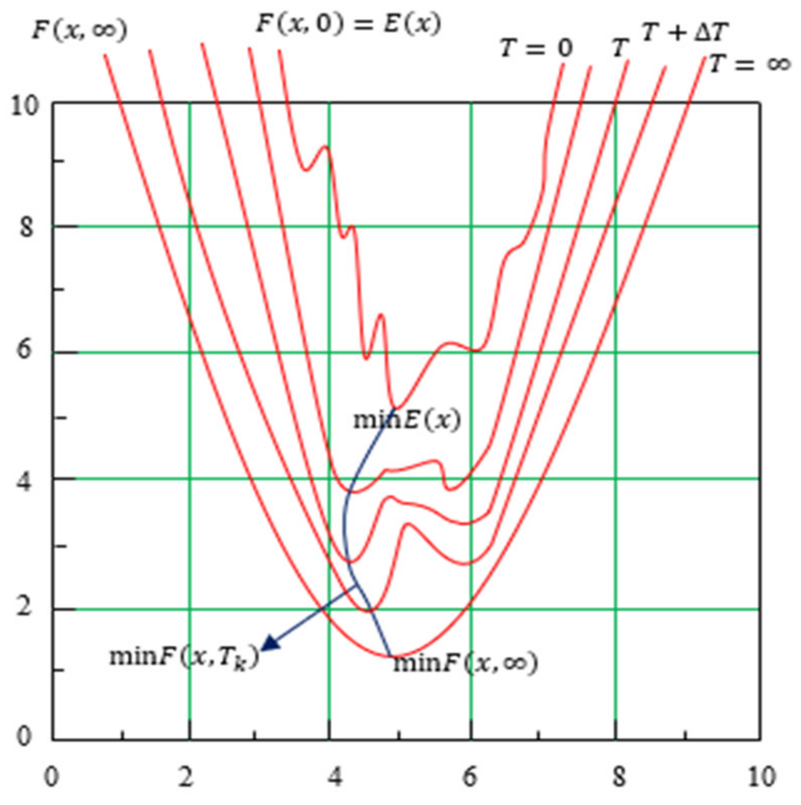
As shown in Figure 2, when solving minimisation problems, m i n E = E x , where E x is the energy of a certain system. When solving this problem with DA, the optimal solution can be obtained from the minima value of the system’s free-energy function. A corresponding free-energy function of the system [29] is constructed as: F x , T = E x T H , where T and H are the temperature and entropy of the system, respectively, and T controls the balance between the energy and entropy of the system. When solving the optimal solution under each T, DA uses the maximum entropy principle in information theory to minimise F x , T , which is essentially to minimise E x . When T slowly approaches zero from a sufficiently large value, F x , T degenerates into the objective function E x . If the above-mentioned process is satisfied, the constructed free-energy function F x , T must meet the following conditions. (1) When T = , the global minimum value of F x , with respect to x is easy to find (if F is a convex function, its global minimum can be easily solved by using some traditional optimisation methods). (2) When T = 0 , F x , 0 = E x . Then, the problem is solved through the following process. The pseudo-code of the process is given in Algorithm 1, which is self-explained.
Algorithm 1 Overview of Deterministic Annealing
1. Set a sufficiently large T 0 T 0 = , k = 0 Solve the optimisation problem m i n F x , T 0 . Let the optimal solution be x m i n T 0 ;
2.  While ( T k > T f )
3.   T k + 1 = c T k ( 0 < c < 1 ) ;
4.  Take x m i n T k as the initial solution, select an iterative method (such as Newton iteration method, conjugate gradient method or gradient descent method) to solve m i n F x , T k + 1 . Let the optimal solution be x m i n T k + 1 ;
5.    X = x m i n T k + 1 ;
6.    k = k + 1 ;
7.  End
8. X is the optimal solution;
9. Return
The process above shows that the basic idea of DA is to establish a mapping φ T , and the image of φ T at a certain point T k is a certain global minimum point of the function F x , T k . When F x , T has a certain continuity, the corresponding global minimum point φ T changes continuously as T decreases from to 0. Under this assumption of continuity, we can take φ T + Δ T as the initial point and use traditional optimisation methods, such as gradient descent, to obtain φ T . By continuously decreasing T, φ 0 , that is, the global minimum of the objective function, can be obtained.
Fox proved that the initialisation of DA should be at a high temperature because deinitialisation at a higher temperature than the initial one can reduce the nonlinear effect. When the temperature is zero, the energy function of the system is directly minimised to produce a non-random solution. The cooling plan has a crucial impact on the performance of this method. Rapid cooling causes a quenching effect, which likely leads to a non-global minimum at zero temperature. Slow cooling can keep the system in equilibrium all the time. Therefore, at zero temperature, the energy configuration of the system is the smallest, and the best solution can be obtained. DA allows the geometric cooling law: T t = ρ T t 1 , 0 < ρ < 1 , and ρ is usually between 0.95 and 0.99. Reference [30] showed that the probability convergence of the global minimum can be achieved when T t = O ( log t 1 ) , where T t is the temperature at time t [31].
If the problem to be solved is an optimisation problem with continuous variables, DA may use the steady optimisation theory’s popular and influential conclusion. Through the mean-field approximation, the most appropriate method is utilised in the optimisation steps at each temperature to select the most unbiased and undeniable solution under given conditions, rather than random probability. Therefore, the time complexity of the algorithm search is much lower than that of the simulated annealing process, and the algorithm can converge quickly. A secondary advantage of DA is that T has fixed minimum and maximum values for any problem. This part of the algorithm is not heuristic, so it can be calculated in principle.
DA has been widely used in travelling salesman problems [32,33] and can efficiently find the optimal path. In recent years, DA has been employed to solve NP-hard problems, such as graph clustering. Reference [34] proposed a deterministic annealing neural network algorithm to solve the graph partitioning problem. Reference [35] presented a Lagrangian-type DA algorithm to solve the maximum clique problem. Some scholars also applied DA to vehicle path planning [36,37].

3.2. Deterministic Annealing Based on Artificial Potential Field

The method of escaping from the local minimum involves randomly searching the surface of the potential energy function and trying to minimise the potential energy function to find a position with lower potential energy than the local minimum where the current robot is stuck. Inspired by the DA process, DA-APF introduces temperature parameters to control the robot’s trajectory, so it can effectively avoid random movement on the surface of the potential energy function. Equations (1) and (5) are reconsidered as follows:
U T a t t q = 1 2 ξ σ 2 q , q t a r g e t α T , σ q , q t a r g e t T σ 0
U T r e p q = 1 2 η 1 ρ q , q o b s t α T 1 ρ 0 2 , | ρ q , q o b s t T ρ 0 0 . | ρ q , q o b s t T > ρ 0
Then,
U T q   = U T a t t q + i = 1 n U T r e p i q ,
where T is the temperature parameter, α is the cooling factor, and 0 < α < 1 . The entropy function of the system is defined as follows:
S = q p q log p q .
Next, the corresponding Lagrangian free-energy potential function is constructed as follows:
E q , T = U T q T S .
Equations (11) and (12) are potential field functions that are improved by introducing the temperature parameter, which can reduce the distance threshold σ 0 between the robot and the target and increase the influence radius ρ 0 of obstacles. In this way, the robot becomes highly sensitive to barriers. In the early stage of path planning, when the temperature is high, the robot focuses on the search and avoidance of blocks. In the late stage of planning, as the temperature decreases slowly, the repulsive force decreases, and the attractive force increases; then, the robot gradually loses ‘interest’ in obstacles until it reaches the target. When the robot falls into the local minimum, the tempering strategy is adopted, and the temperature stops decreasing and rises instead. The repulsive force of the obstacle to the robot suddenly increases to ‘pop’ the robot out of the local minimum. Therefore, the robot can achieve fast pathfinding and efficient obstacle avoidance by increasing the potential influence of obstacles and raising the priority of minimum local departure in path planning. Algorithm 2 is used as the core part of local path planning.
Algorithm 2 DA-APF for local path planning
1. Set P = P 0 , T = T 0 . Here, T 0 is large enough;
2. Start annealing. Set T i + 1 = α T i ( 0 < α < 1 ) , use the conjugate gradient method to obtain the p i corresponding to each T i ;
3. While  ( T i > T f )
4. If  ( p i  P )  Then
5.   Execute the gradient descent potential guided strategy to obtain P ˜ . Let P = P ˜ ;
6. If  ( p i is in the neighbourhood of P under a certain T i )  Then
7.   If  d p i , P ρ 0  Then
8.   Execute the tempering strategy. Let T i + 1 = T i / α until escape. Update P ˜ using gradient descent. Let P = P ˜ ;
9.   Else
10.    Let P = P ˜ ;
11. If U T P ˜ U T P 0  Then
12.  Obtain the optimal path P m i n . Let P = P m i n ;
13. Let T i + 1 = α T i ;
14. End
15. P is the optimal or near-optimal path solution;
16. Return
DA-APF has the real-time performance of the APF method and the stable convergence of the DA method. Before planning the path, the global minimum on the surface of the improved potential energy function is obtained by the DA method, thereby optimising the initial path to the greatest extent. Then, on the basis of the trend of the potential field, path planning is guided by gradient descent. If the robot falls into a local minimum in the process, the tempering strategy is used to help it escape, and annealing is continued until the obstacle avoidance is completed or the target is reached.

4. Simulation Results

In this section, path planning was designed for a complex environment with convex polygon or nonconvex polygon obstacles, and parameter testing and algorithm comparative simulation were performed to illustrate the excellent performance of the proposed DA-APF. The simulation studies were carried out in MATLAB (R2016a) under Windows 10 on a laptop with 2.50 GHz AMD Ryzen 5 4600U CPU and 16.0 GB RAM. The experiment was based on the simulator developed by MATLAB. The simulated robot was a differential-driven mobile platform equipped with six distance sensors evenly distributed on the front, left, right, left and right sides of the robot, and the detection distance was about three meters. All 2D environments contained the local minima that may prevent the robot from reaching the target. In the simulation results, the starting points were represented by S, the targets were represented by T, and their coordinates were (50, 50) and (450, 450), respectively. The size of the environment was 500 cm × 500 cm. The distance and time units were centimeters and seconds, respectively. For all simulations, the parameters were set as follows: ξ = 1 , η = 3 , σ 0 = 100 , ρ 0 = 30 , T 0 = 10000 , α = 0.98
A-Star (A*), GA and SA were used as comparison algorithms in this paper. In Review [38], these algorithms were systematically introduced. A* is a classical path planning algorithm based on cost function minimisation. Reference [39] filtered the nodes in the close-list through the constructor to avoid the problems of many nodes, long distance and large turning angle in the sawtooth and cross paths generated by the traditional A* algorithm. By introducing the radar threat estimation function and a 3D bidirectional sector multilayer variable-step search strategy, Reference [40] proposed an optimal penetration path planning method that aims to satisfy the waypoint accuracy and the algorithm search efficiency. GA is a global optimisation algorithm that has strong robustness and is widely used. Reference [41] proposed an innovative APF algorithm and developed an enhanced genetic algorithm (EGA) to improve the initial path in continuous space and find the optimal path between the start and destination. SA has strong local optimisation ability and can make the search process avoid falling into the local optimal solution. Reference [42] proposed a method based on SA and Dijkstra to obtain the path trajectory of each robot and calculated the shortest path between each region according to the global map information and the Boolean specification.

4.1. Environment I

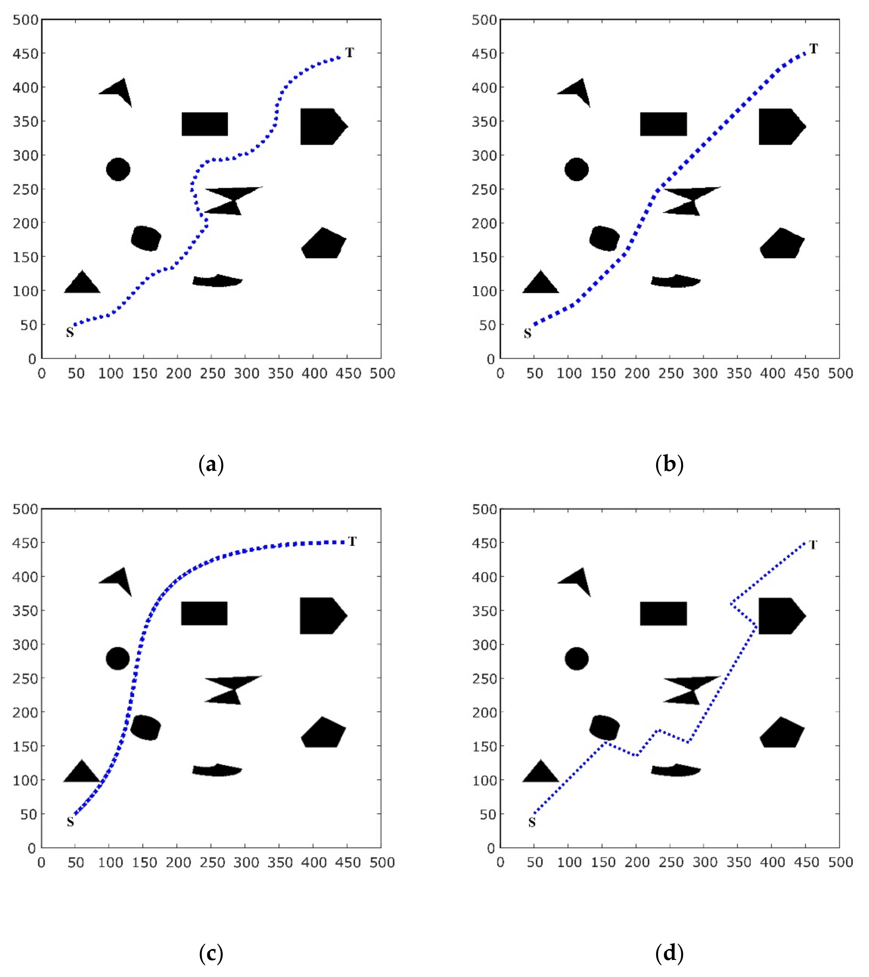
Environment I has nine convex polygon or nonconvex polygon obstacles. When obstacles are detected, DA-APF and the three other algorithms can avoid obstacles and reach the target. Therefore, Figure 3 shows no collision. Notably, the path smoothness of GA is relatively inferior to that of the three other algorithms. Table 1 lists the simulation results for path planning time, path length and pathfinding success rate. The results show that the success rate of all algorithms is 100%. In terms of time and path length, DA-APF is better than GA and SA. A* almost finds the shortest path in this environment, but it consumes the longest time and lacks specific real-time performance.

4.2. Environment II

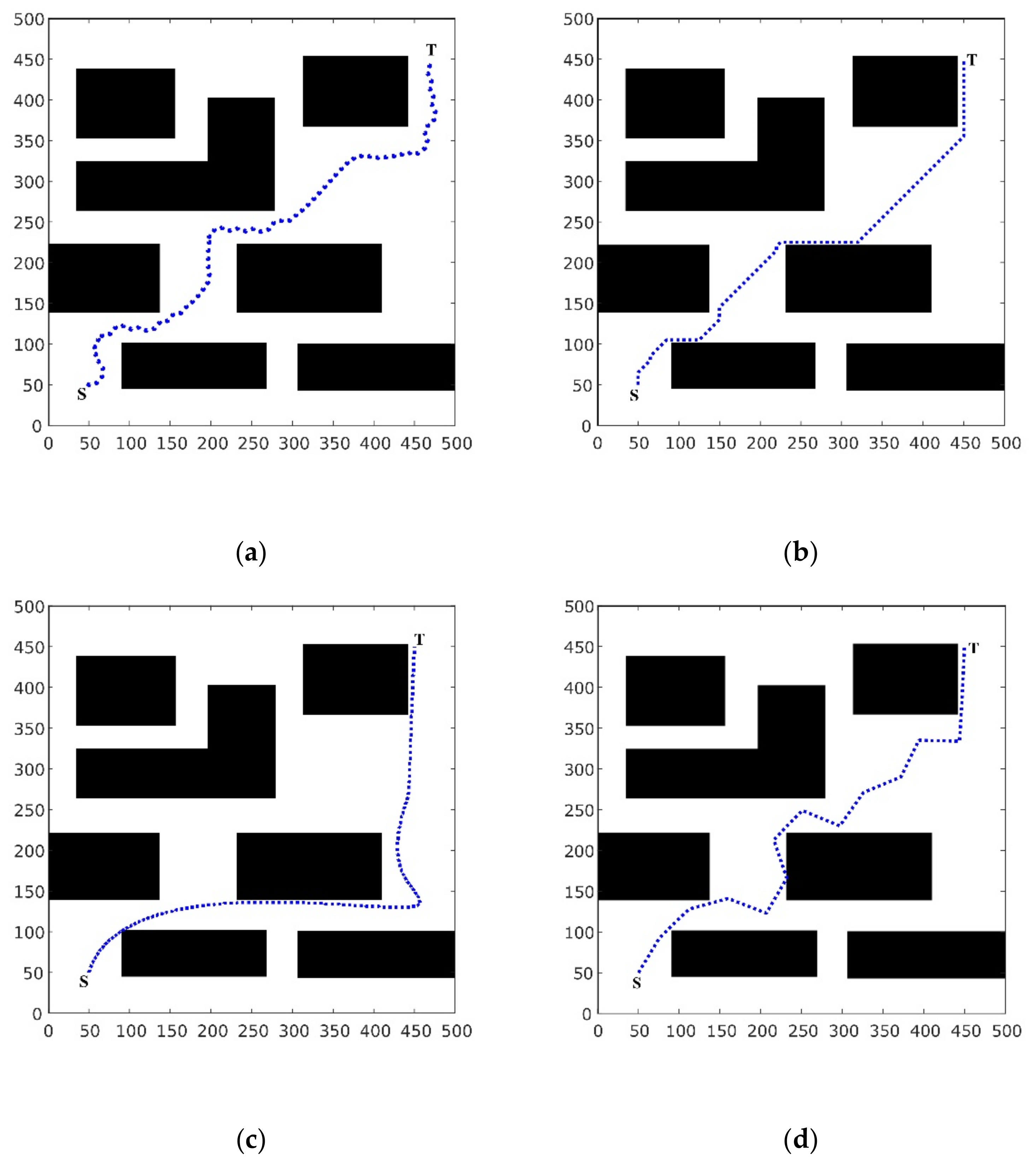
Compared with Environment I, Environment II has a higher volume of obstacles and arrangement density and is more extensive. Figure 4 shows the simulation results for DA-APF and the three comparison algorithms. The path smoothness of SA is the worst, and the path obtained by DA-APF maintains a certain safe distance from the obstacle, which is an advantage that the three other algorithms do not have. Table 2 lists the simulation results for path planning time, path length and pathfinding success rate in Environment II. The table indicates that the all-around performance of GA is the worst (when parameters NoOfGenerations and PopulationSize are set to 20 and 50, respectively), and the implementation of DA-APF is better than that of GA and SA. Compared with the path length of A*, the path length of DA-APF is almost the same, but its path planning time is much shorter.

4.3. Environment III

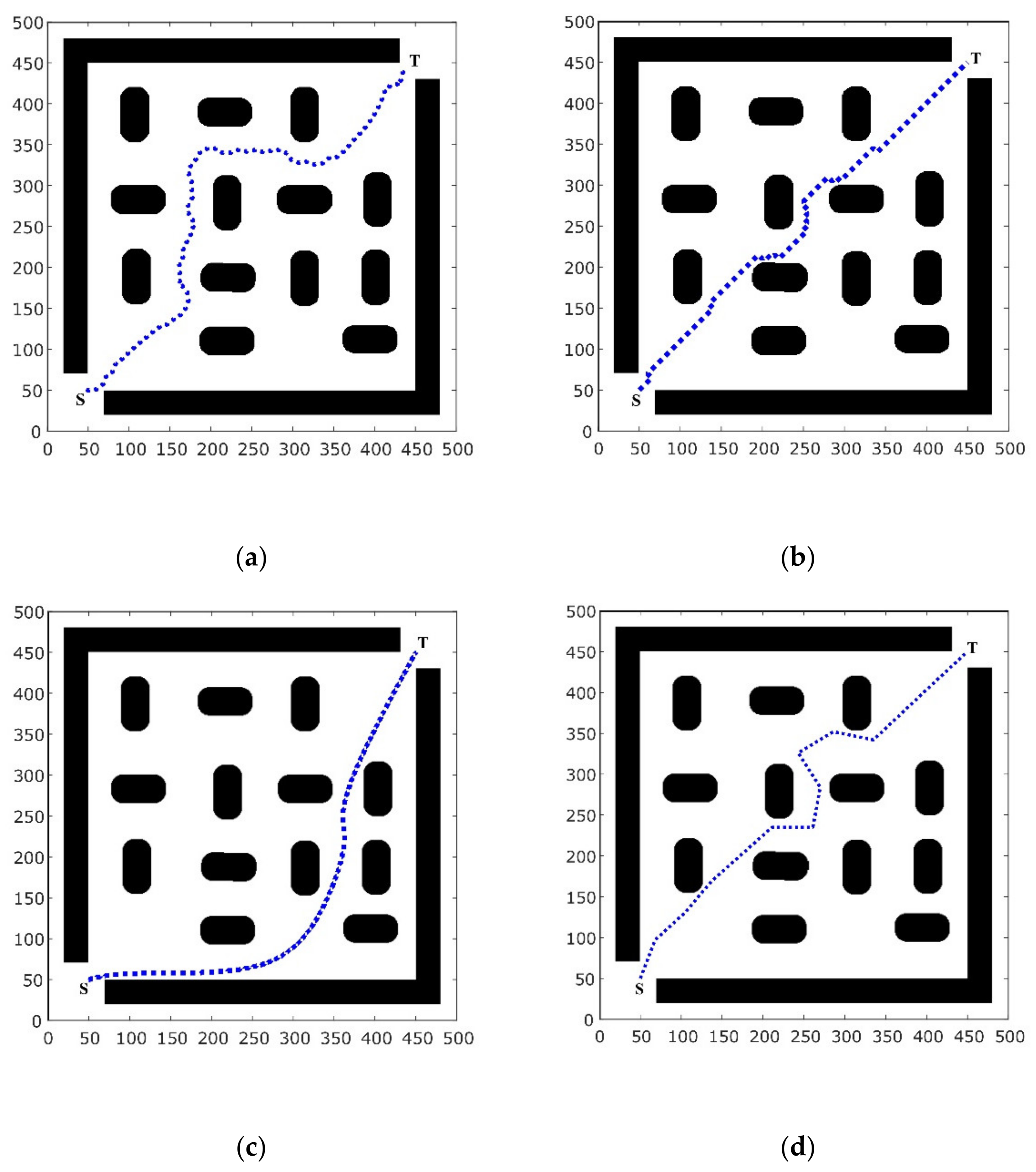
Environment III is more complex than Environment II. It is an almost closed scene with a large number of obstacles and irregular arrangement. Figure 5 shows Environment III and its simulation results. The path obtained by DA-APF is better than those obtained by the three other algorithms in terms of smoothness and safe distance from obstacles. Table 3 shows some quantitative simulation results for Environment III. The table indicates that except for GA, the three other algorithms’ success rate is 100%. DA-APF consumes the least time, and the path length of A* is the shortest, but it is not far from that of DA-APF. Comprehensive comparison shows that DA-APF still performs the best.

4.4. Environment IV

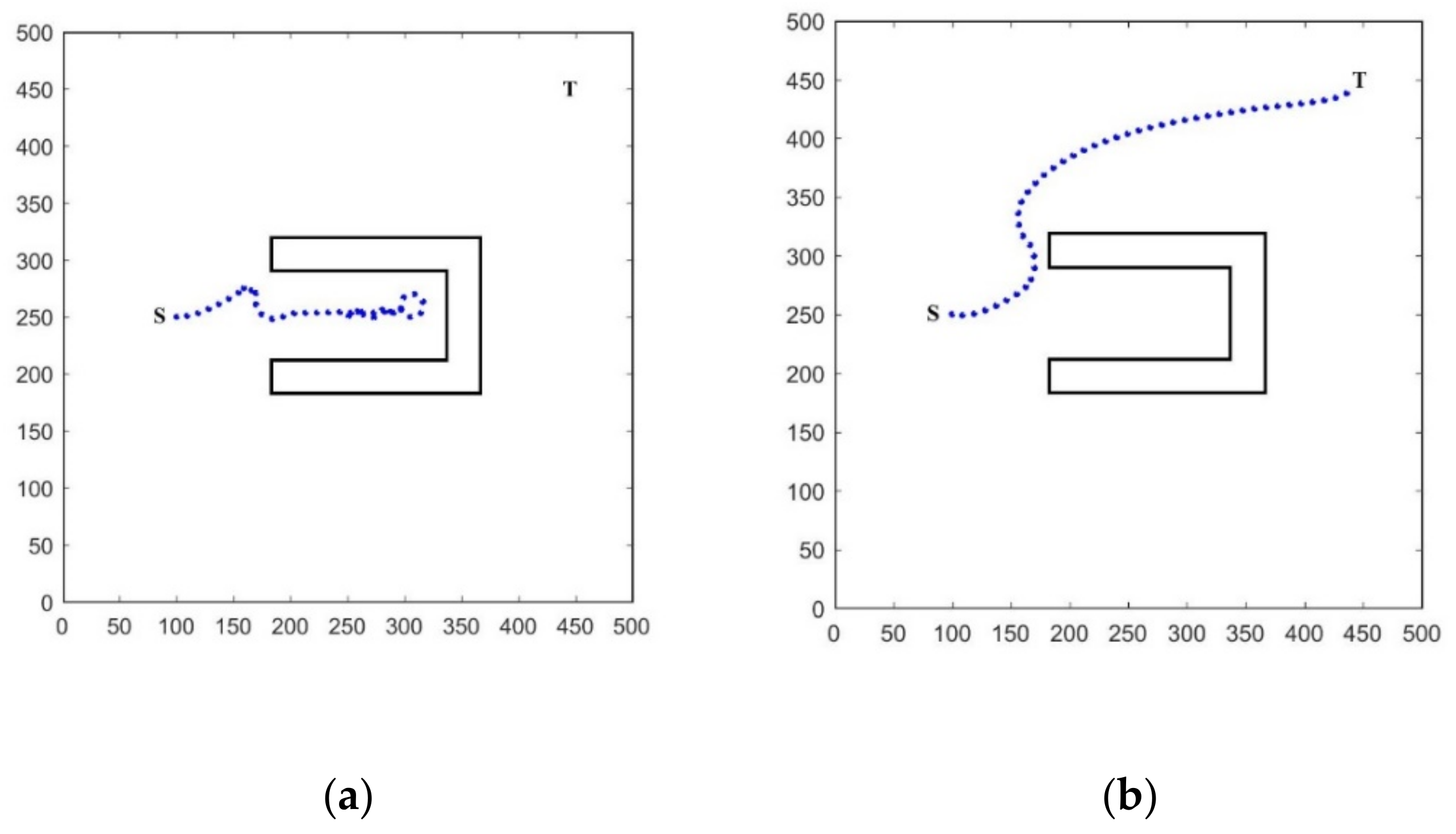
Environment IV is a classic U-shaped obstacle, and it contains strong local minima points. The focus of this section is to show that the proposed DA-APF can cope with local minima. For analysis convenience, the starting point is set to (100, 250). As shown in Figure 6a, standard APF cannot easily complete obstacle avoidance. The robot is trapped in a U-shaped obstacle and finally presents a repeated closed-loop trajectory; hence, it cannot escape. Meanwhile, the proposed DA-APF can solve the local minima problem, as shown in Figure 6b, and the robot does not even enter the U-shaped obstacle. The quantitative analysis in Table 4 indicates that DA-APF has obvious advantages over standard APF.

4.5. Further Performance Analysis

The initial temperature ( T 0 ) and cooling coefficient ( α ) were analysed to investigate the effect of annealing parameters on the performance of DA-APF. The obstacle environment was simplified to make it suitable for the study of annealing parameters. The simulation results are shown in Table 5. The table indicates that the selection of initialisation temperatures and cooling coefficients has a great influence on the performance of DA-APF. When DA-APF was initialised at a sufficiently high temperature, the convergence speed and success rate of DA-APF were high, indicating good performance. By contrast, when the initial temperature was low, the two performance indexes were low (i.e., poor performance), which is also consistent with the basic idea that DA must be initialised at high temperatures. Similarly, the table indicates that DA-APF performs well at high cooling coefficients, but when the coefficient decreases, the performance of the algorithm worsens. The analysis of the number of iterations reveals that when α is less than the theoretical value, the annealing process becomes unstable and may even cause quenching. The analysis of the success rates indicates that a small α accelerates the tempering in the obstacle avoidance process, resulting in the failure of obstacle avoidance or deviation from the target.

5. Conclusions

In this paper, a robot static path planning algorithm inspired by DA (called DA-APF) was proposed. The algorithm is heuristic and has great application potential in embedded systems with limited computing resources. DA-APF is also an improvement of the standard APF algorithm, and it can solve the deadlock problem faced by robots in potential field modelling. The core of the algorithm is to use annealing and tempering strategies to drive and avoid obstacles. Simulation results show that DA-APF can handle environments with multiple convex or non-convex polygon obstacles, and the method performs best at high-temperature initialisation and low cooling rates. Compared with heuristic path planning algorithms, such as GA and SA, DA-APF has advantages in planning time, path length and path smoothness. Compared with the standard APF method, the improved DA-APF can easily adapt to the U-shaped obstacle environment. Notably, the paths obtained by DA-APF are relatively safe. However, considering that robots need pose transformation in the real world, the distance threshold must be studied further for it to become more in line with the real environment. This paper focused on static environments, and the next research direction will be path planning in dynamic and mixed-obstacle environments.

Author Contributions

Conceptualization, Q.G.; methodology, J.Q.; software, J.D.; writing—original draft preparation, J.D. and J.Q.; writing—review and editing, Z.W., H.Y. and C.Z.; supervision, Q.G.; funding acquisition, Z.W. All authors have read and agreed to the published version of the manuscript.

Funding

This research was funded by the NSFC under grant nos. 61803279, in part by the Qing Lan Project of Jiangsu, in part by the China Postdoctoral Science Foundation under grant nos. 2020M671596 and 2021M692369, in part by the Suzhou Science and Technology Development Plan Project (Key Industry Technology Innovation) under grant no. SYG202114, and in part by the Open Project Funding from Anhui Province Key Laboratory of Intelligent Building and Building Energy Saving, Anhui Jianzhu University, under grant no. IBES2021KF08.

Institutional Review Board Statement

Not applicable.

Informed Consent Statement

Not applicable.

Data Availability Statement

Not applicable.

Conflicts of Interest

The authors declare no conflict of interest.

References

  1. Tuncer, A.; Yildirim, M. Dynamic path planning of mobile robots with improved genetic algorithm. Comput. Electr. Eng. 2012, 38, 1564–1572. [Google Scholar] [CrossRef]
  2. Tsai, C.C.; Huang, H.C.; Chan, C.K. Parallel elite genetic algorithm and its application to global path planning for autonomous robot navigation. IEEE Trans. Ind. Electron. 2011, 58, 4813–4821. [Google Scholar] [CrossRef]
  3. Miao, H.; Tian, Y.C. Dynamic robot path planning using an enhanced simulated annealing approach. Appl. Math. Comput. 2013, 222, 420–437. [Google Scholar] [CrossRef] [Green Version]
  4. Behnck, L.P.; Doering, D.; Pereira, C.E.; Rettberg, A. A modified simulated annealing algorithm for SUAVs path planning. IFAC J. Syst. Control 2015, 48, 63–68. [Google Scholar] [CrossRef]
  5. Liu, J.; Yang, J.; Liu, H.; Tian, X.; Gao, M. An improved ant colony algorithm for robot path planning. Soft Comput. 2017, 21, 5829–5839. [Google Scholar] [CrossRef]
  6. Ma, Y.N.; Gong, Y.J.; Xiao, C.F.; Gao, Y.; Zhang, J. Path planning for autonomous underwater vehicles: An ant colony algorithm incorporating alarm pheromone. IEEE Trans. Veh. Technol. 2018, 68, 141–154. [Google Scholar] [CrossRef]
  7. Abbasi, A.; MahmoudZadeh, S.; Yazdani, A.; Moshayedi, A.J. Feasibility assessment of Kian-I mobile robot for autonomous navigation. Neural Comput. Appl. 2022, 34, 1199–1218. [Google Scholar] [CrossRef]
  8. Li, G.; Chou, W. Path planning for mobile robot using self-adaptive learning particle swarm optimization. Sci. China Inform. Sci. 2018, 61, 1–18. [Google Scholar] [CrossRef] [Green Version]
  9. Teli, T.A.; Wani, M.A. A fuzzy based local minima avoidance path planning in autonomous robots. Int. J. Inf. Technol. 2021, 13, 33–40. [Google Scholar] [CrossRef]
  10. Byrne, S.; Naeem, W.; Ferguson, S. Improved APF strategies for dual-arm local motion planning. Trans. Inst. Meas. Control 2015, 37, 73–90. [Google Scholar] [CrossRef] [Green Version]
  11. Ma’Arif, A.; Rahmaniar, W.; Vera, M.A.M.; Nuryono, A.A.; Majdoubi, R.; Çakan, A. Artificial potential field algorithm for obstacle avoidance in uav quadrotor for dynamic environment. In Proceedings of the 2021 IEEE International Conference on Communication, Networks and Satellite (COMNETSAT), Purwokerto, Indonesia, 17–18 July 2021; pp. 184–189. [Google Scholar]
  12. Abdalla, T.Y.; Abed, A.A.; Ahmed, A.A. Mobile robot navigation using PSO-optimized fuzzy artificial potential field with fuzzy control. J. Intell. Fuzzy Syst. 2017, 32, 3893–3908. [Google Scholar] [CrossRef]
  13. Guerra, M.; Efimov, D.; Zheng, G.; Perruquetti, W. Avoiding local minima in the potential field method using input-to-state stability. Control Eng. Pract. 2016, 55, 174–184. [Google Scholar] [CrossRef] [Green Version]
  14. Khatib, O. Real-time obstacle avoidance for manipulators and mobile robots. In Proceedings of the 1985 IEEE International Conference on Robotics and Automation, St. Louis, MO, USA, 25 March 1985; pp. 500–505. [Google Scholar]
  15. Zhang, T.; Zhu, Y.; Song, J. Real-time motion planning for mobile robots by means of artificial potential field method in unknown environment. Int. J. Rob. Res. 2010, 37, 384–400. [Google Scholar]
  16. Zhu, Q.; Yan, Y.; Xing, Z. Robot path planning based on artificial potential field approach with simulated annealing. In Proceedings of the Sixth International Conference on Intelligent Systems Design and Applications, Jian, China, 16–18 October 2006; pp. 622–627. [Google Scholar]
  17. Weerakoon, T.; Ishii, K.; Nassiraei, A.A.F. An artificial potential field based mobile robot navigation method to prevent from deadlock. J. Artif. Intell. Soft 2015, 5, 189–203. [Google Scholar] [CrossRef] [Green Version]
  18. Zhang, J.; Yan, J.; Zhang, P. Fixed-wing UAV formation control design with collision avoidance based on an improved artificial potential field. IEEE Access 2018, 6, 78342–78351. [Google Scholar] [CrossRef]
  19. Szczepanski, R.; Bereit, A.; Tarczewski, T. Efficient local path planning algorithm using artificial potential field supported by augmented reality. Energies 2021, 14, 6642. [Google Scholar] [CrossRef]
  20. Zappulla, R.; Park, H.; Virgili-Llop, J.; Romano, M. Real-time autonomous spacecraft proximity maneuvers and docking using an adaptive artificial potential field approach. IEEE Trans. Control Syst. Technol. 2018, 27, 2598–2605. [Google Scholar] [CrossRef]
  21. Shin, Y.; Kim, E. Hybrid path planning using positioning risk and artificial potential fields. Aerosp. Sci. Technol. 2021, 112, 106640. [Google Scholar] [CrossRef]
  22. Orozco-Rosas, U.; Montiel, O.; Sepúlveda, R. Mobile robot path planning using membrane evolutionary artificial potential field. Appl. Soft Comput. 2019, 77, 236–251. [Google Scholar] [CrossRef]
  23. Huang, Y.; Ding, H.; Zhang, Y.; Wang, H.; Cao, D.; Xu, N.; Hu, C. A motion planning and tracking framework for autonomous vehicles based on artificial potential field elaborated resistance network approach. IEEE Trans. Ind. Electron. 2019, 67, 1376–1386. [Google Scholar] [CrossRef]
  24. Sharma, K.; Doriya, R. Coordination of multi-robot path planning for warehouse application using smart approach for iden-tifying destinations. Intel. Serv. Robot. 2021, 14, 313–325. [Google Scholar] [CrossRef]
  25. Yan, F. Autonomous vehicle routing problem solution based on artificial potential field with parallel ant colony optimization (ACO) algorithm. Pattern Recognit. Lett. 2018, 116, 195–199. [Google Scholar] [CrossRef]
  26. Guo, J.; Gao, Y.; Cui, G. Path planning of mobile robot based on improved potential field. J. Inf. Technol. 2013, 12, 2188. [Google Scholar] [CrossRef] [Green Version]
  27. Rose, K.; Gurewitz, E.; Fox, G.C. Statistical mechanics and phase transitions in clustering. Phys. Rev. Lett. 1990, 65, 945–948. [Google Scholar] [CrossRef]
  28. Wu, Z.; Karimi, H.R.; Dang, C. A deterministic annealing neural network algorithm for the minimum concave cost transportation problem. IEEE Trans. Neural Netw. Learn. Syst. 2019, 31, 4354–4366. [Google Scholar] [CrossRef]
  29. Gibbs, J.W. On the equilibrium of heterogeneous substances. Trans. Conn. Acad. Arts Sci. 1879, 2, 300–320. [Google Scholar] [CrossRef]
  30. Geman, S.; Geman, D. Stochastic relaxation, Gibbs distributions, and the Bayesian restoration of images. IEEE Trans. Pattern Anal. Mach. Intell. 1984, 6, 721–741. [Google Scholar] [CrossRef]
  31. Rose, K.; Gurewitz, E.; Fox, G.C. Vector quantization by deterministic annealing. IEEE Trans. Inf. Theory 1992, 38, 1249–1257. [Google Scholar] [CrossRef]
  32. Dang, C.; Xu, L. A Lagrange multiplier and Hopfield-type barrier function method for the traveling salesman problem. Neural Comput. 2002, 14, 303–324. [Google Scholar] [CrossRef]
  33. Wu, Z.; Gao, Q.; Jiang, B.; Karimi, H.R. Solving the production transportation problem via a deterministic annealing neural network method. Appl. Math. Comput. 2021, 411, 126518. [Google Scholar] [CrossRef]
  34. Wu, Z.; Karimi, H.R.; Dang, C. An approximation algorithm for graph partitioning via deterministic annealing neural network. Neural Netw. 2019, 117, 191–200. [Google Scholar] [CrossRef] [PubMed]
  35. Dai, J.; Wu, Z.; Karimi, H.R.; Jiang, B.; Lu, G. An Approximation Lagrangian-based Algorithm for the Maximum Clique Problem via Deterministic Annealing Neural Network. J. Frankl. Inst. 2022, 359, 6080–6098. [Google Scholar] [CrossRef]
  36. Molenbruch, Y.; Braekers, K.; Caris, A. Operational effects of service level variations for the dial-a-ride problem. Cent. Eur. J. Oper. Res. 2017, 25, 71–90. [Google Scholar] [CrossRef]
  37. Baranwal, M.; Parekh, P.M.; Marla, L.; Salapaka, S.M.; Beck, C.L. Vehicle routing problem with time windows: A deterministic annealing approach. In Proceedings of the IEEE 2016 American Control Conference (ACC), Boston, MA, USA, 6–8 July 2016; pp. 790–795. [Google Scholar]
  38. Patle, B.K.; Pandey, A.; Parhi, D.R.K.; Jagadeesh, A. A review: On path planning strategies for navigation of mobile robot. Def. Technol. 2019, 15, 582–606. [Google Scholar] [CrossRef]
  39. Tang, G.; Tang, C.; Claramunt, C.; Hu, X.; Zhou, P. Geometric A-star algorithm: An improved A-star algorithm for AGV path planning in a port environment. IEEE Access 2021, 9, 59196–59210. [Google Scholar] [CrossRef]
  40. Zhang, Z.; Wu, J.; Dai, J.; He, C. Optimal path planning with modified A-Star algorithm for stealth unmanned aerial vehicles in 3D network radar environment. Proc. Inst. Mech. Eng., Part G J. Aerosp. Eng. 2022, 236, 72–81. [Google Scholar] [CrossRef]
  41. Nazarahari, M.; Khanmirza, E.; Doostie, S. Multi-objective multi-robot path planning in continuous environment using an enhanced genetic algorithm. Expert Syst. Appl. 2019, 115, 106–120. [Google Scholar] [CrossRef]
  42. Shi, W.; He, Z.; Tang, W.; Liu, W.; Ma, Z. Path planning of multi-robot systems with boolean specifications based on simulated annealing. IEEE Rob. Autom. Lett. 2022, 7, 6091–6098. [Google Scholar] [CrossRef]
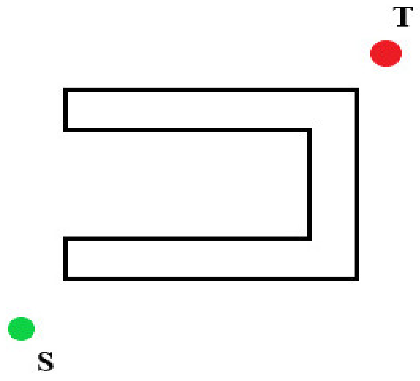
Figure 1. U-shaped obstacle.
Machines 10 00600 g001
Figure 2. Iterative process of deterministic annealing.
Machines 10 00600 g002
Figure 3. Environment I. The figures contain the simulation paths of the following algorithms: (a) DA-APF, (b) A*, (c) GA and (d) SA.
Machines 10 00600 g003
Figure 4. Environment II. The figures contain the simulation paths of the following algorithms: (a) DA-APF, (b) A*, (c) GA and (d) SA.
Machines 10 00600 g004
Figure 5. Environment III. The figures contain the simulation paths of the following algorithms: (a) DA-APF, (b) A*, (c) GA and (d) SA.
Machines 10 00600 g005
Figure 6. Environment IV. The figures contain the simulation paths of the following algorithms: (a) APF and (b) DA-APF.
Machines 10 00600 g006
Table 1. Performance results for Environment I (mean values from 50 runs for all algorithms).
AlgorithmsTimePath LengthSuccess Rate/%
DA-APF1.57629100
A*7.53576100
GA2.07710100
SA2.08673100
Table 2. Performance results for Environment II (mean values from 50 runs for all algorithms).
AlgorithmsTimePath LengthSuccess Rate/%
DA-APF1.79712100
A*10.18675100
GA3.3377984
SA1.59763100
Table 3. Performance results for Environment III (mean values from 50 runs for all algorithms).
AlgorithmsTimePath LengthSuccess Rate/%
DA-APF1.72680100
A*6.56651100
GA1.8170294
SA2.15687100
Table 4. Performance results for Environment IV (mean values from 50 runs for all algorithms).
AlgorithmsTimePath LengthSuccess Rate/%
APF4.15 *492 *24
DA-APF1.12447100
* When the robot successfully reaches the target.
Table 5. Performance results for DA-APF (mean values from 10 runs).
  T 0 α Average Number of IterationsSuccess Rate/%
9999 0.98610100
0.97621100
0.96624100
0.95133980
0.942550
2000 0.98324540
0.97325610
0.96173820
0.954760
0.942300
Publisher’s Note: MDPI stays neutral with regard to jurisdictional claims in published maps and institutional affiliations.