Abstract
This work addresses the end-effector trajectory-tracking force and motion control of a three-dimensional three-link robot considering measurement noises. The last two links of the manipulator are considered as structurally flexible. An absolute coordinate approach is used while obtaining the dynamic equations to avoid complex dynamic equations. In this approach, each link is modeled as if there is no connection between the links. Then, joint connections are expressed as constraint equations. After that, these constraint equations are used in dynamic equations to decrease the number of equations. Then, the resulting dynamic equations are transformed into a form which is suitable for controller design. Furthermore, the dynamic equations are divided as pseudostatic equilibrium and deviation equations. The control torques resulting from the pseudostatic equilibrium and the elastic deflections are obtained easily as the solution of algebraic equations. On the other hand, the control torques corresponding to the deviations are obtained without any linearization. Encoders, strain gauges, position sensors and force and moment sensors are required for measurements. Low pass filters are considered for the sensors. For the crossover frequencies of the sensors, low and high values are chosen to observe the filtering effect on the robot output.
1. Introduction
Flexible manipulators (FMs) have become very important because of demand for low energy consumption, high accuracy, high speed, low cost and low weight. Since the dynamics of these FMs show high coupling and high nonlinearity, obtaining dynamic equations (DEs) and controlling the FM are complicated matters. The recent literature is mentioned in the subsequent paragraphs.
Mosayebi, Ghayour and Sadigh [1] addressed a motion control (MC) algorithm utilizing an output redefinition. They considered a planar single-link (SL) FM. Pereira, Trapero, Diaz and Feliu [2] developed an adaptive control approach for the MC of a planar SL FM. Wang and Kang [3] developed an adaptive neural network technique for the MC of a planar SL FM. Latip, Husain, Mohamed and Basri [4] used an adaptive proportional plus integral plus derivative control technique for the MC of a planar SL FM. Zhang, Yang, Sun and Fang [5] utilized an adaptive fuzzy control approach for the MC of a planar SL FM. Dong, He, Ma, Zhang and Li [6] designed an iterative learning control using proportional plus derivative control for the MC of a planar SL FM. Cambera and Feliu-Batlle [7] presented a control approach utilizing feedback linearization for the MC of a planar SL FM. They considered only the first elastic mode in their dynamic model. Sun, Gao, He and Yu [8] used a fuzzy neural network strategy for the MC of a planar SL FM. Ozguney and Burkan [9] presented a sliding mode control utilizing a fuzzy logic approach to determine the control gains for the MC of a planar SL FM. Qiu, Wang, Zhang and Han [10] considered proportional plus derivative control law and adaptive fuzzy control law for the MC of a spatial SL FM.
Abe [11] considered a feedforward control method for the point-to-point MC of an FM. They considered a planar SL FM and a planar two-link (TL) robot with a flexible first link. Forbes and Damaren [12] presented an optimization method. They utilized a closed-loop (CL) H2 norm as the objective function. The MC of a planar SL FM and a planar TL FM were taken into consideration. Qiu, Li and Zhang [13] designed a minimum variance self-tuning controller and a fuzzy neural network controller for the MC of a planar SL FM. Zhang, Zhang, Zhang and Dong [14] utilized a fuzzy proportional plus integral plus derivative control for the MC of a planar TL FM. Khan and Kara [15] used a neural fuzzy approach for the MC of a planar TL FM. Pradhan and Subudhi [16] used a self-tuning proportional plus integral plus derivative control for the MC of a planar TL FM. Pedro and Smith [17] developed a proportional plus integral plus derivative control with an iterative learning technique for the MC of a planar TL FM. Yang and Zhong [18] considered a terminal sliding mode method for the MC of a planar TL FM. Wang, Niu, Yang and Xu [19] designed a controller by combining the terminal sliding mode and output redefinition for the MC of a planar TL FM. Rahmani and Belkheiri [20] designed an adaptive control method by using joint space variables for the MC of a planar TL FM. They utilized a stable inversion and a linear compensator in their control law. Xu [21] utilized a singular perturbation approach to divide the system dynamics as slow and fast dynamics. Disturbance observer and neural networks were used for the slow dynamics and the sliding mode was considered for the fast dynamics. The control law was developed by using joint space variables for the MC of a planar TL FM. Shafei, Bahrami and Talebi [22] designed a sliding mode control and a Lyapunov function considering planar TL FM and spatial TL FM. Kilicaslan, Ider, and Ozgoren [23] have proposed a task space MC law for a spatial three-link FM.
SL FMs [1,2,3,4,5,6,7,8,9,10], planar FMs [1,2,3,4,5,6,7,8,9,11,12,13,14,15,16,17,18,19,20,21], joint space control [20,21], inverse dynamics techniques [18,20], and singular perturbation techniques [21] utilized for the development of control approaches in recent works have been summarized in the previous paragraphs.
It is assumed that link stiffness is large enough in the singular perturbation approach. If this is not the case, a high gain is needed to separate the dynamics as fast and slow. This may cause a spillover of dynamics, which is not modeled. Since the inverse dynamics approach uses iterative procedures, it needs more computation time. Although joint angles may be controlled so as not to face a non-minimum phase system, controlling the end-effector (EE) variables is better in order to decrease the task errors. The dynamics of planar FMs are much simpler than the dynamics of spatial FMs. Finally, SL FM is too simple to observe the couplings of the rigid and elastic variables.
Moreover, the recent studies mentioned above [1,2,3,4,5,6,7,8,9,10,11,12,13,14,15,16,17,18,19,20,21,22,23] consider only the MC of FMs. However, in industry, there are various applications in which the tip point of the robot has a trajectory in a constrained environment such as deburring, grinding, surface finishing and assembly. In these applications, the hybrid force and motion control (FMC) of FMs is required. Therefore, the performance of the FMC of FMs needs to be checked.
Kilicaslan, Ozgoren, and Ider [24] proposed a task space FMC law and they considered a planar TL FM with an elastic forearm in the simulations. However, the performance of a control method needs to be checked using a spatial FM, as the DEs of spatial FMs are much more complicated than the DEs of planar FMs. In the present work, the proposed method given in [24] is extended to spatial FMs. A spatial three-link robot whose last TLs are elastic are used to inspect the efficiency of the control technique. Additionally, noises in measurements are also taken into consideration.
To avoid complex DEs, each link is modeled as if there is no connection between the links. After that, constraint equations are written for the connections of the links. Then, these constraint equations are used in DEs to decrease the number of equations. After that, the resulting DEs are transformed into an alternative form which is the proper form for controller design.
DEs are separated as pseudostatic equilibrium and deviation equations. Control torques corresponding to pseudostatic equilibrium and elastic deflections are obtained by merely solving a set of algebraic equations. Control torques corresponding to deviations are obtained without needing any linearization. Encoders, strain gauges, position sensors, and force and moment sensors are required for the measurement of joint variables, elastic variables, EE position variables, and contact forces and/or moments, respectively [25]. Low pass filters are considered for the sensors. For the crossover frequencies of the sensors, low and high values are chosen to observe the filtering effect on the robot output.
The control method used in this work has many advantages. One advantage is that at the pseudostatic equilibrium, elastic variables and torques can be calculated easily by using algebraic equations. Another advantage is that, though the related matrices are dependent on the position and velocity level variables, there are linear relationships between accelerations and torques. Therefore, by the placement of the CL poles, properly linear control approaches can be applied without linearization to reduce deviations from the pseudostatic equilibrium. So, the system’s non-minimum phase characteristics are managed in this way. As a result of this, this method can be applied easily in comparison to techniques that need linearization. Particularly if the degree-of-freedom (DOF) of the manipulator is high, this feature of the technique is very beneficial. The third advantage is that since the EE variables are used as the controlled variables, better tracking accuracy may be obtained when compared to the methods that use joint angular variables as the controlled variables.
2. Previous and Present Studies Comparison
Based on the previous section, the previous and present studies are compared in a tabular form by considering the usability of the studies in applications.
For the comparison of the usability of the previous and present studies, firstly, limitations and/or disadvantages of the FMs or control techniques or dynamic models utilized in previous works are given in Table 1. Secondly, limitations and/or disadvantages of the previous studies are listed in Table 2. Lastly, advantages of the FM, control technique, and dynamic model utilized in the present work are given in Table 3.

Table 1.
Limitations and/or disadvantages of the FMs or control techniques or dynamic models utilized in previous works.
Table 2.
Limitations and/or disadvantages of previous works.
Table 3.
Advantages of the FM, control technique, and dynamic model utilized in present work.
Space stations, the chemical industry, the military, nuclear plants, and underwater applications are the basic areas in which spatial FMs have been increasingly utilized. However, there are few studies considering spatial FMs. Therefore, the performance of a control method needs to be checked using spatial FMs as the DEs of spatial FMs are much more complicated than the DEs of planar FMs. Additionally, in industry, there are various applications in which the tip point of the robot has a trajectory in a constrained environment such as deburring, grinding, surface finishing, and assembly. In these applications the hybrid FMC of FMs is required. Therefore, the performance of the FMC of spatial FMs needs to be checked.
3. Dynamic Modeling
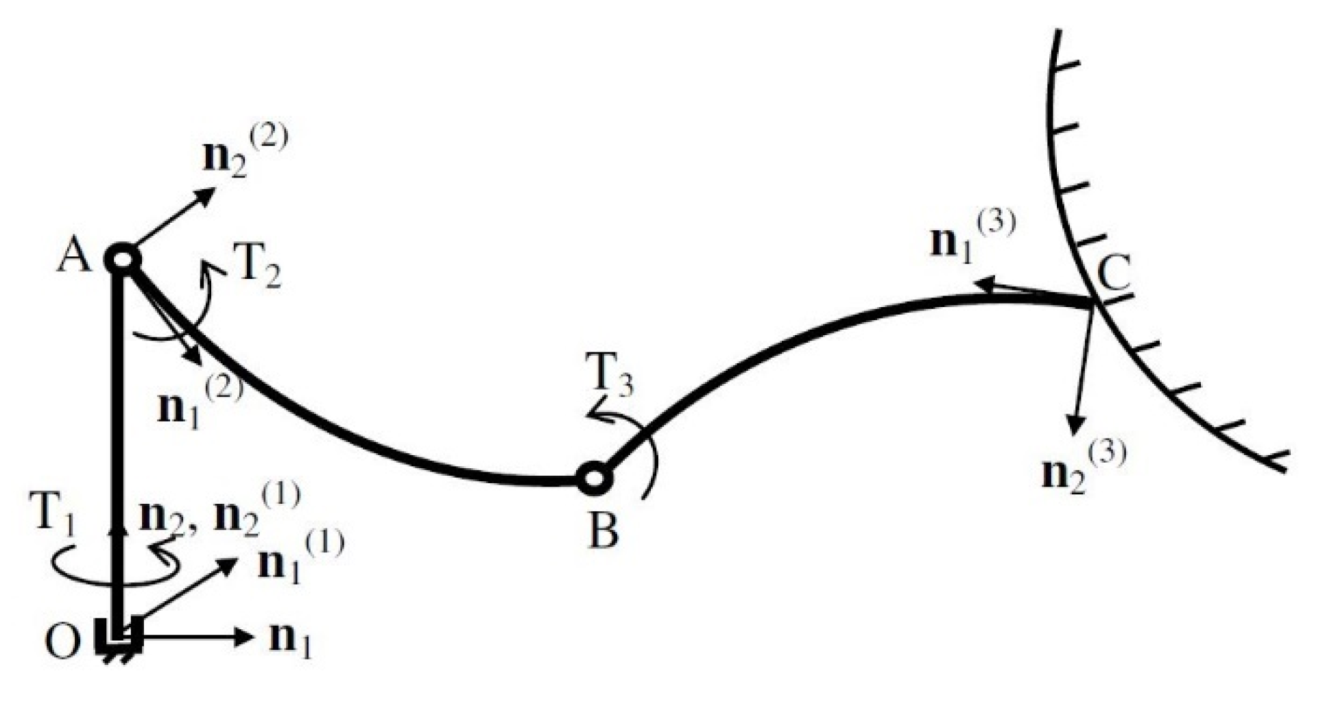
A three-dimensional three-link robot depicted in Figure 1 is considered. The last TLs of the manipulator are considered as structurally flexible. The absolute coordinate approach is used while obtaining the DEs of the FM to avoid complex DEs. In this approach, each link is modeled by utilizing its rigid and flexible DOF based on the fixed frame as if there is no connection between the links. Then, joint connections are written as constraint equations.
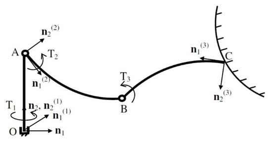
Figure 1.
Spatial three-link FM.
Link 2 and link 3 are assumed to be flexible while link 1 is taken as rigid. Actuators at points A and B and the payload at point C and EE are considered as lumped masses mA, mB, and mC, respectively. Revolute joints are used for the connections.
ℑ(1) represents the frame at point O of link 1, ℑ(2) represents the frame at point A of link 2, ℑ(3) represents the frame at point C of link 3, and ℑ = ℑ(0) represents the fixed frame. Each frame unit vector is denoted by ni(j) where superscript j (j = 0, 1, 2, 3) refers to the frame number and subscript i (i = 1, 2, 3) stands for the axis number.
For flexible link Euler–Bernoulli beams are utilized. It is assumed that deformation displacements stay in the elastic zone. They are expressed with respect to the link frames. Finite element modeling is used for them. In finite element modeling, two-node beam elements are considered for discretization. Deformation rotations and deformation displacements of the centerlines are used as the nodal variables. From the solution of each link’s free vibration problem, nodal variables are transformed to modal variables to decrease the number of variables.
Link 1 and link 2 have no translational DOFs, while link 3 possesses three translational DOFs; link 1 has a single rotational DOF while link 2 and link 3 have three rotational DOFs; link 1 has no modal DOF since it is rigid, while link 2 has m(2) modal DOFs and link 3 possesses m(3) modal DOFs, as seen from Figure 1. Some of the abovementioned translational and rotational motions are dependent on each other due to the motion limitations imposed by the joints. Therefore, the corresponding constraints are taken into consideration before writing out separate constraint equations for simplicity.
By using the remaining constraint equations for the joint connections, the DE of the spatial FM can be written as [25]
Here, y denotes the vector of generalized speeds. fc, fs, fg, fe, and Q are the vectors of generalized contact forces, structural stiffness forces, gravitational forces, external forces, and Coriolis, gyroscopic and centrifugal forces, respectively. B stands for the Jacobian matrix for constraints. M designates the generalized mass matrix. μ represents the vector of constraint forces resulting from the joint constraints. They can be written as:
Components of y are represented as:
In the above equations, y(1), y(2), and y(3) denote the vectors of generalized speeds of links 1, 2 and 3, respectively; β1 stands for the link 1 angle of rotation, and represent the angular velocities of links 2 and 3 written in their own frames, respectively; η(2) and η(3) designate the vectors of modal variables of links 2 and 3, respectively; and ζ(3) stands for the position vector from point O to point C, which is between the origins of the frames attached to the ground and link 3. Although n scalar equations (n = 10 + m(2) + m(3)) can be obtained from Equation (1), there are n + c unknowns in these equations. This means that c constraint equations are needed.
For the rest of the joint constraints, seven expressions can be formed (i.e., c = 7). Due to the revolute joint at point A, the angular velocities of link 1 about the n1(2) and n2(2) axes must be equal to the angular velocities of link 2 about the n1(2) and n2(2) axes. Due to the revolute joint at point B, the velocities of link 2 in the n1, n2, and n3 axes must be equal to the velocities of link 3 in the n1, n2, and n3 axes, and the angular velocities of link 2 about the n1(2B) and n2(2B) axes should be equal to the angular velocities of link 3 about the n1(2B) and n2(2B) axes. ℑ(2B) represents the frame at point B of link 2 where the unit vector n3(2B) is along the rotation axis of the revolute joint at B.
Constraint equations can be put into the following form:
The above expression includes c scalar equations which are at velocity levels. In these constraint equations, the number of unknowns is n which is the same as the unknowns of Equation (1). Acceleration level constraint equations are obtained as follows by taking the derivative of the above constraint equations:
The DEs of the whole FM are obtained by forming the augmented matrix composed of Equations (1) and (6) as follows:
One of the goals of this study is to control the EE position of the FM. To this end, the EE position variables and modal variables of the links are important. As a result of this, the components of y vector can be rearranged as:
where ym stands for the rearranged representation of y. and , m = m(2) + m(3), can be called primary variables, while κ ∈ ℜc can be called secondary variables. Components of the above vector are defined as follows:
By utilizing the constraint equations, the secondary variables may be eliminated from the DE of the FM. As a result of this, a convenient form of the DE is acquired in terms of the primary variables.
The reordered form of Equation (7) compatible with ym is obtained by rearranging its columns and rows consistently:
Here, the subscript m indicates the rearranged representation of the related vector or matrix. Expanded forms of the above equations are presented as:
In the above equations, by partitioning fmc, fme, fms, and Qm, submatrices of Lm, Hm, Sm, and Cm are acquired, respectively. λ denotes the vector of Lagrange multipliers (contact forces) resulting from the contact between a surface and the EE. T is the vector of torques.
By using the following equation
secondary variables are represented as functions of primary variables
With the help of Equations (15) and (17), can also be represented as a function of primary variables:
Utilizing Equations (17) and (18) in Equations (12)–(14), the dynamic behavior of the FM is defined by primary variables and μ as given below:
Here, Zζ, Zη, Zκ, Yζ, Yη, Yκ, Gζ, Gη, Gκ, Kηη, Vζζ, Vζη, Vηζ, Vηη, Vκζ, Vκη, Nζζ, Nζη, Nηζ, Nηη, Nκζ, and Nκη, are expressed as:
With the help of Equation (21), μ may be represented by , , , , and λ as:
By substituting Equation (34) in Equations (19) and (20), the DEs of the spatial FM are defined by the primary variables only as given in the following:
In the above two equations Fζ, Fη, Eζ, Eη, Dζ, Dη, Bζζ, Bζη, Bηζ, Bηη, Aζζ, Aζη, Aηζ, and Aηη are given as:
Features of the spatial FM model considered are tabulated as given in Table 4.
Table 4.
Features of the spatial FM model considered.
4. Control Law
For the control approach, DEs are decomposed as pseudostatic equilibrium equations and deviation equations that represent the deviations from the pseudostatic equilibrium. The pseudostatic equilibrium is a hypothetical condition. In this condition, the velocity and acceleration of the EE and the contact forces and/or moments have their reference values and, at the same time, the elastic deflections are instantaneously constant. The hypothetical pseudostatic equilibrium condition may be considered as an equivalent gravitational field including reference and gravitational acceleration vectors. By using the EE motion variables, the modal variables and the contact force/moment components, torques for the pseudostatic equilibrium and the stabilization of the deviations are obtained. EE motion variables can be measured by utilizing convenient sensors. By using joint and modal variables measurements, EE motion variables can also be obtained if the EE motion sensors are not available. The number of modes used in calculations defines the accuracy of this representation [25].
The EE constraint equations due to contact with a surface may be expressed as:
The derivative of the above equations may be given by:
where ϕ ∈ ℜk, ζ ∈ ℜn and Φ = ∂ϕ/∂ζ. Because of the constraints, position of the EE is given by:
Here, s ∈ ℜn-k denotes the independent variable vector and can be called the “contact surface coordinates”. The derivative of the above equation gives:
Here, denotes the contact surface tangential velocity vector. Ψ is given as:
By substituting Equation (47) into Equation (45), the following expression can be written:
As is not identically equal to zero, from Equation (49) the following equation is written:
The differentiation of Equation (47) gives:
Substitutions of Equations (47) and (51) into Equations (35) and (36) give:
where , , , , , , , and .
The vectors of contact surface coordinates, modal coordinates, control torques, and Lagrange multipliers (contact forces) are separated as:
where s* represents the reference contact surface coordinates, s′ stands for the deviation from the reference contact surface coordinates, η* is the pseudostatic modal coordinates, η′ designates the deviation from the pseudostatic modal coordinates, λ* denotes the reference contact forces at the EE contact constraints, λ′ represents the deviation from the reference contact forces at the EE contact constraints, T* denotes the torques needed for the pseudostatic equilibrium and T′ stands for the torques needed for stabilization to minimize the deviation from the reference contact surface coordinates, pseudostatic modal coordinates, and desired contact forces at the EE contact constraints.
At the pseudostatic equilibrium, it is assumed that Rkl, Ykl, Kkk, Dk, Ek, and Fk (k = ζ, η, and l = ζ, η) are frozen at their instantaneous values and η* is an instantaneously constant vector of elastic deflections due to , , λ* and gravitational acceleration, g. So, the next expressions are written at the pseudostatic equilibrium:
At the pseudostatic equilibrium, Equations (52) and (53) are given by:
Using Equations (56) and (57), η* and T* are obtained in terms of g and , , λ* as follows:
The actuation singularity of the FM occurs if the above inverse does not exist.
Deviation equations that represent the deviations from the pseudostatic equilibrium are acquired by the subtraction of Equation (56) and Equation (57) from Equation (52) and Equation (53), respectively, as:
In Equations (59) and (60), δζ and δη can be considered as disturbances, expressed as:
To stabilize the deviation equations and to minimize the deviations at the minimum level in the case of a disturbance, T′ can be formed as follows [24,25]:
Here, γ′ is the impulse (integral) of the vector of contact force deviation and S is the gain matrix. γ′ is calculated by:
One can conclude from Equations (62) and (63) that the integral controller is utilized for the contact forces and the proportional plus derivative controller is utilized for the motion force. Stabilizing torques are acquired if the gain matrix can be chosen conveniently. Equations (59) and (60) may be represented by:
where
Therefore, deviation equations are represented in terms of state variables as follows:
where W ∈ ℜ2(n-m)-k is assumed to be vector of disturbances. T′ ∈ ℜn is the vector of correction torques. F ∈ ℜ2[(n-m)-k]×n and E ∈ ℜ2[(n-m)-k]×2[(n-m)-k] are proper matrices. x′ ∈ ℜ2(n-m)-k is the deviation equations state vector. Their explicit forms are given by:
The substitution of Equation (62) into Equation (68) gives:
where Γ = E − FS. Here, S is selected such that poles of the above CL deviational system (DS) make the DS stable. For the selection of S, the pole placement technique is utilized. The S value is updated through the trajectory of the FM.
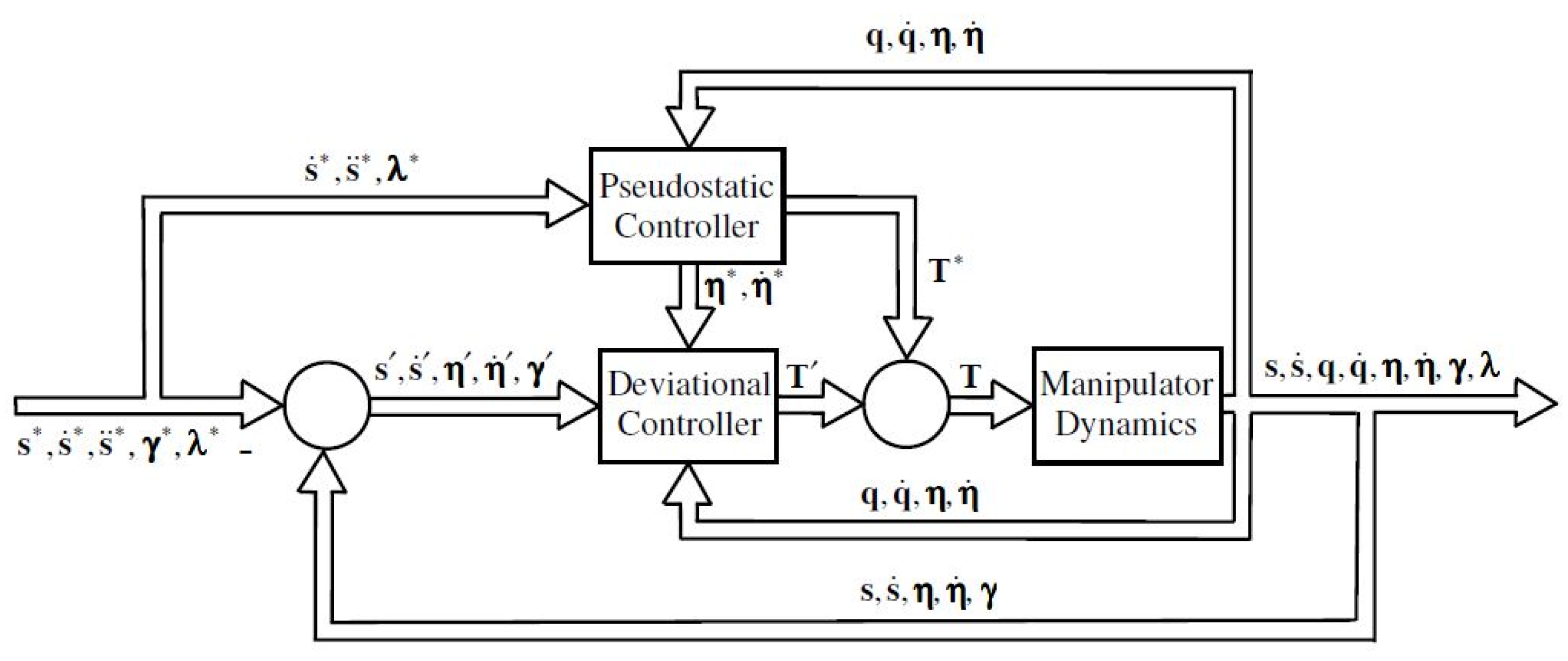
The control approach block diagram can be drawn as in Figure 2. Here, q and denote joint variables and their derivatives, respectively.
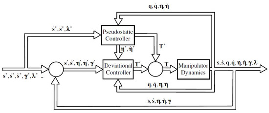
Figure 2.
Control method block diagram.
5. Stability
Assumption 1.
Equations (35) and (36) describe the dynamics of the FM and they are nonlinear equations. Although Equation (70) has a nonlinear structure because of the position and velocity-dependent coefficients, for the deviational forms of the state variables, this equation can be considered in the form of a linear equation. As a result of this, the CL DS given in Equation (70) may be expressed by a linear time-varying (LTV) DS whose coefficients are:
Here, y*(t) results from s*(t) and λ*(t). When the controller is constructed for LTV DS by keeping ||x′(t)|| small enough, then this requirement is satisfied. This means that LTV DSs are made stable by properly selecting S providing that ||x′(0)|| and ||W(t)||are small enough. As a result of this, if x(t) is in the vicinity of x*(t), then DS will also be made stable. Thus, coefficients of DS and LTV DS will be near to each other through the trajectory [23,24]. This means that:
Assumption 2.
Measurement noises are assumed to be Gaussian white noises with small standard deviations. By utilizing a low pass filter with first-order dynamics, measurements are filtered. It is assumed that the filter’s crossover frequencies are large enough such that poles corresponding to filter dynamics are far away from the fundamental poles. Therefore, filter dynamics are ignored.
Remark 1.
The theorem given below is for the stability of the LTV DS expressed by Equation (71). However, because of Assumption 1, the theorem can also be used for the stability of the DS expressed by Equation (70). This means that, for small disturbances and initial deviations, LTV DS stability indicates DS stability [23,24]. Therefore, computations of E, F, and S can be obtained by use of instantly measured variables of y and . Therefore, burdensome and repetitive a priori calculations to obtain y*(t) that corresponds to s*(t) and λ*(t) are not needed. Moreover, storing y*(t) is not necessary for online calculations.
Theorem 1.
If S is chosen by satisfying the following three criteria and if the Assumptions 1 and 2 are satisfied, then, CL DS expressed by Equation (70) will be asymptotically stable.
- (1)
- and
- (2)
- and
- (3)
- ,
where. κi(t) is the ith eigenvalue of Γ. mc andσ0 are real constants.
Proof.
See [23,24]. □
6. Numerical Example
In this section, the FMC of the spatial FM is simulated by considering the DEs and the control method given in Section 3 and Section 4, respectively. In the simulations, measurement noises of the sensors are also taken into considerations.
In the control method, it is assumed that the state variables are measured. The state variables are the azimuth angle and the elevation angle coordinates and the rates of them, the modal variables of links 2 and 3 and the rates of them, and the integral of Lagrange multipliers. Since the Lagrange multipliers are measured in real applications, the integral of the generated noise is taken before adding it to the impulse of the Lagrange multipliers.
To filter noises in measured variables, a low pass filter is introduced. Its first-order dynamics can be described by:
Here, ωc stands for the filter crossover frequency.
Material properties of the links are given in Table 5. The cross-sections of the links are square. The point masses representing actuators at points A and B, and payload and EE at point C are 1.5 kg, 1 kg and 2 kg, respectively. The number of finite elements is taken as five for flexible links. Shear deformations are ignored due to slender links. The first torsional mode natural frequencies of links 2 and 3 are 2995.713 rad/s and 3209.693 rad/s, respectively, and first axial mode natural frequencies of links 2 and 3 are 5344.135 rad/s and 5725.859 rad/s, respectively. This means that the torsional and axial modes are stiff. Therefore, torsional and axial modes are also ignored. Bending modes in the 12 and 13 planes are considered. Clamped-free boundary conditions are applied for the bending modes. The first two bending modes are used. Therefore, the total number of modal variables corresponding to links 2 and 3 is 4. In other words, m(2) = m(3) = 4. Bending modes’ natural frequencies are given in Table 6.
Table 5.
Material properties of the links.
Table 6.
Bending modes’ natural frequencies.
A fourth-order Runge–Kutta technique is applied for solving the DE. MATLAB® is utilized for programming.
A curve on a spherical surface is followed by the EE. Therefore, the constraint is expressed as a function of the EE position variable as:
where ζ1c denotes the sphere coordinate in the n1 direction, ζ2c stands for the sphere coordinate in the n2 direction, ζ3c represents the sphere coordinate in the n3 direction, and R denotes the sphere radius. Thus, the angular spherical coordinate variables s1 and s2 and the EE position variables in the fixed frame n can be combined by the following equations:
where s1 is called the azimuth angle and s2 is called the elevation angle. A polynomial of the ninth-order is considered as a reference trajectory for the azimuth and the elevation angles. Continuous boundary conditions up to the snap are obtained by using this polynomial. It is given by:
where depending on the value of i, si* is the reference azimuth or elevation angle, si0* is the initial value of the reference azimuth or elevation angle, sif* is the final value of the reference azimuth or elevation angle, and tf denotes the time to terminate the motion. tf = 10 s is used in this case.
The desired contact force that is formed by utilizing a cycloidal increase, a dwell, and a cycloidal comeback is expressed as:
where λ* is the reference contact force, λ0* is the constant value of the reference contact force, t1 is the time to finish cycloidal rise motion, and t2 is the time to start the cycloidal return motion. Continuous boundary conditions are also obtained by using this polynomial. t1, t2, and tf are considered as 1.5 s, 8.5 s, and 10 s, respectively. λ0* is used as 50 N.
The following procedure is used for the placement of the poles: Magnitudes of m pole pairs are selected near the natural frequencies of the flexible links. Angles of these m pole pairs are selected to attach a synthetic damping to the elastic modes. The remaining poles are chosen to obtain an adequate achievement by using trial and error.
After a few trials, convenient CL system natural frequency and damping ratio pairs are found as ωn1 = 10 rad/s, ωn2 = 20 rad/s, ωn3 = 30 rad/s, ωn4,5 = 43 rad/s, ωn6,7 = 44 rad/s, ωn8,9 = 268 rad/s, ωn10,11 = 276 rad/s and ζdi = 0.85 (i = 1, 2, …, 11). Notably, (1/500) s is chosen as the sampling time.
Choosing the crossover frequency of the measurement noise filters is important. In general, for better filtering, the crossover frequency should be small. However, the addition of the filter increases the system order, and this may attenuate the relative stability of the system. So, it is better to select a crossover frequency large enough compared to the dominant poles’ magnitudes. In this work, this reality is considered while selecting the crossover frequencies. To show the effect of the crossover frequency on the output, the FMC of the FM is simulated two times by using different crossover frequencies for each simulation.
Random numbers having normal distribution, specific standard deviation, and zero mean are utilized to generate measurement noises. It is assumed that the mean value of each variable has 1% deviation, and this is used to acquire the standard deviation of the associated variable. Moreover, 150 rad/s and 250 rad/s are selected as the filters’ crossover frequencies for the first and second simulations, respectively.
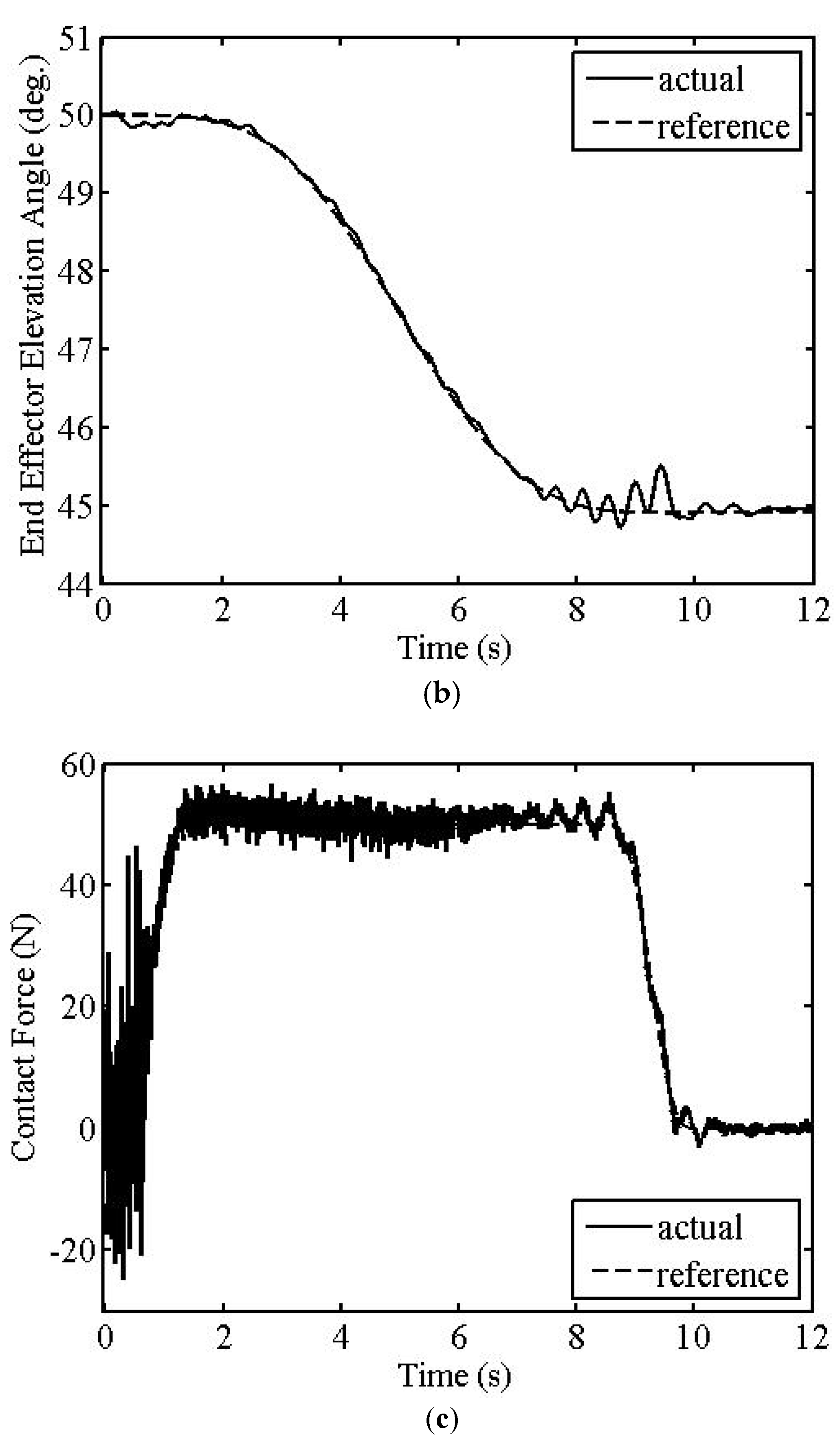
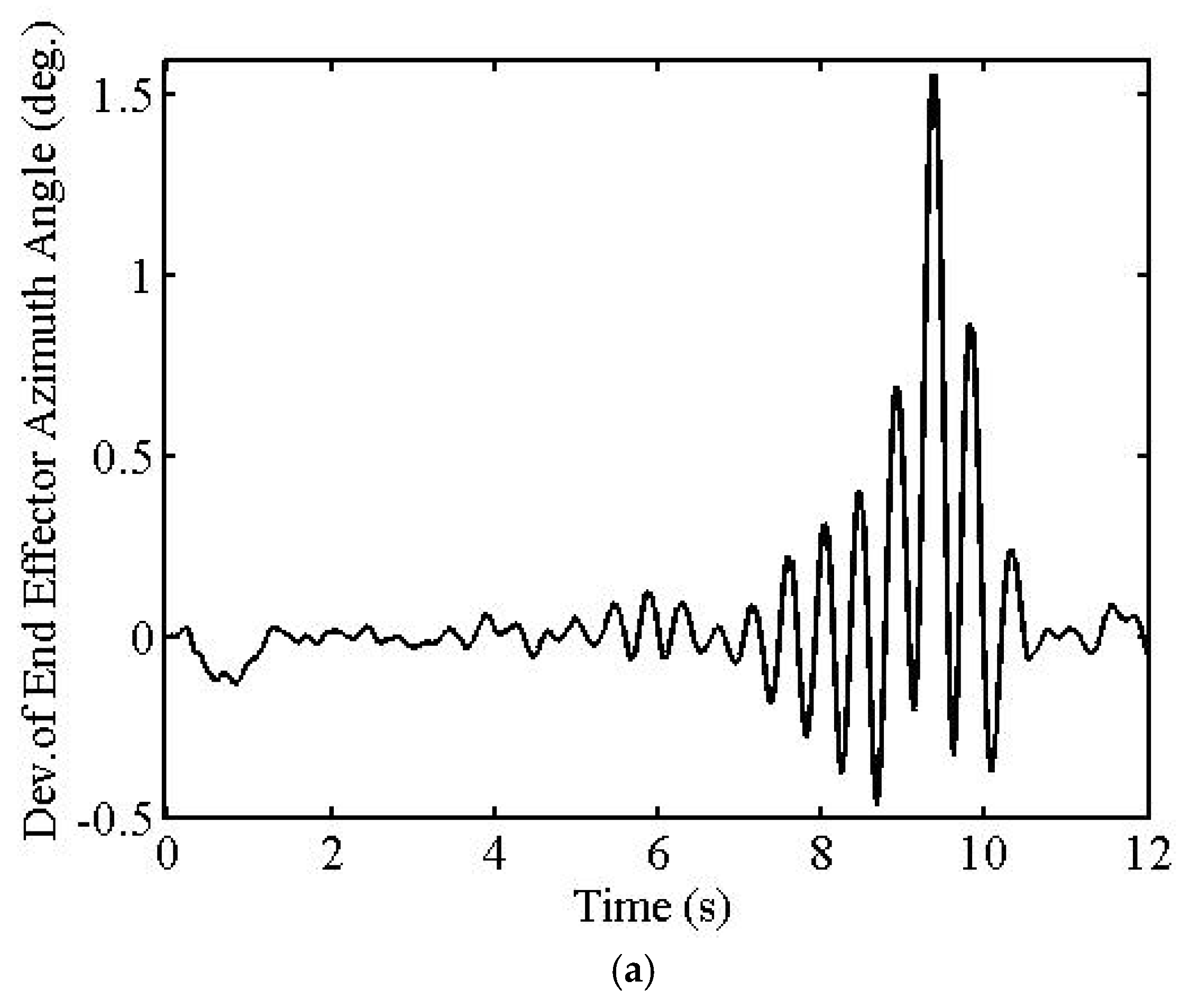
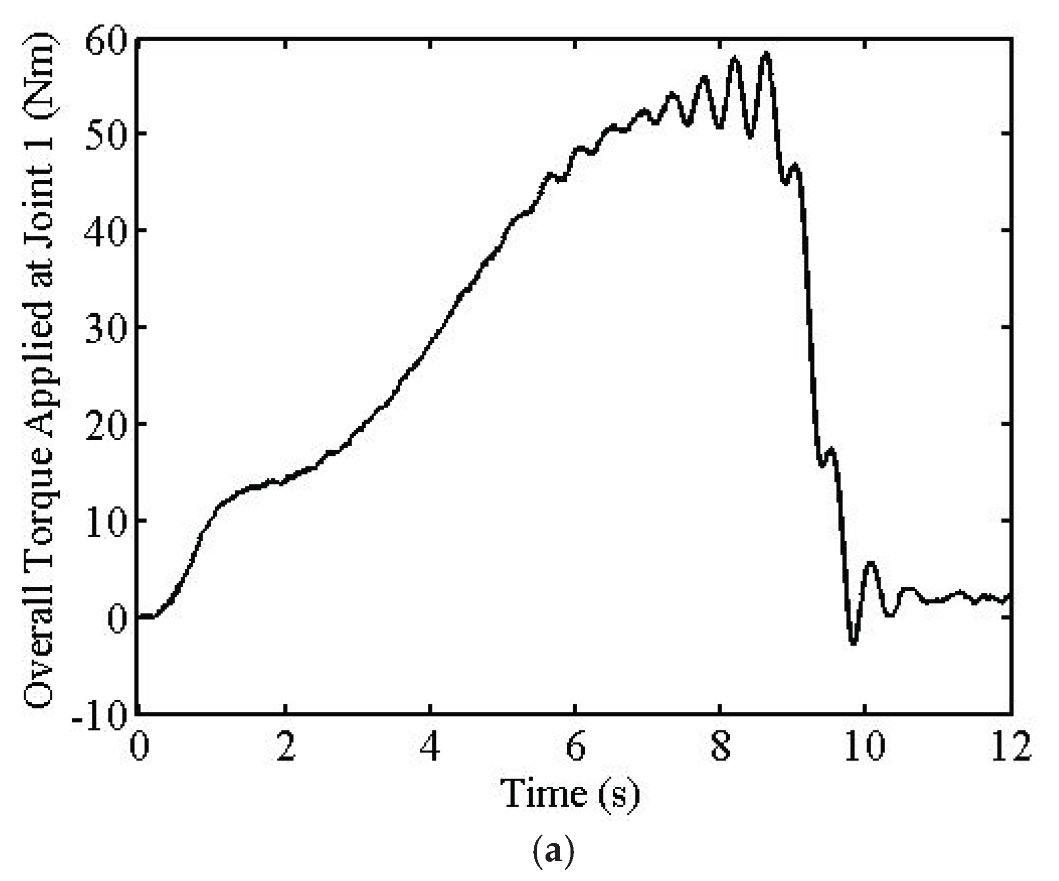
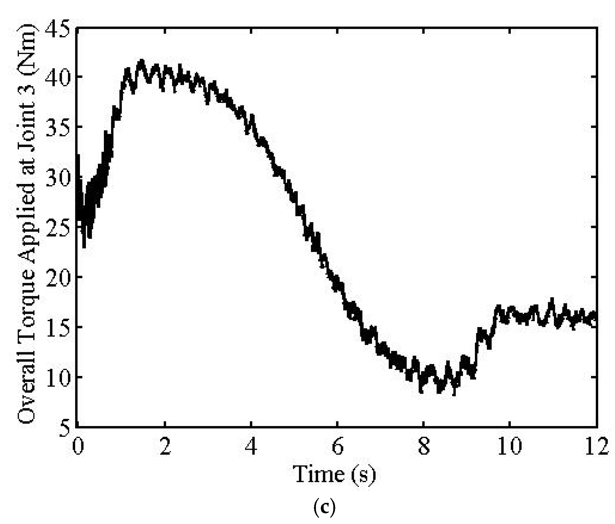
The first simulation results are given in Figure 3, Figure 4 and Figure 5. Tracking error maximum values in the azimuth and elevation angles of the EE are 1.559° and 0.603°, respectively, as seen from Figure 3a,b and Figure 4a,b. The simulations also show that the maximum contact force error value is 6.585 N after the trajectory is settled, as seen from Figure 3c and Figure 4c. The maximum overall torque values do not exceed 170 Nm, as seen from Figure 5.
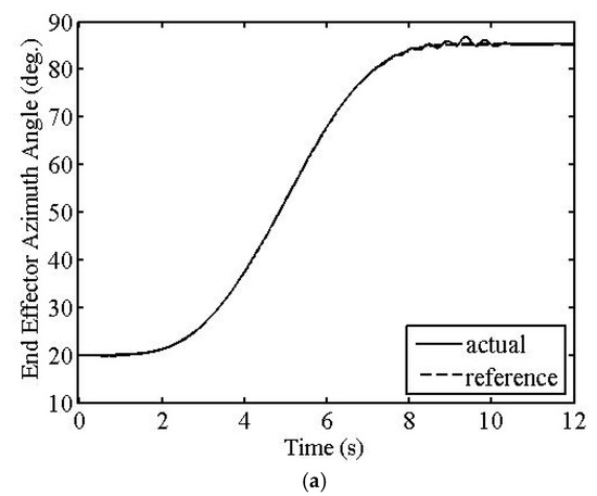
Figure 3.
First simulation results. Azimuth angle (a), elevation angle (b), and contact force (c) of EE.

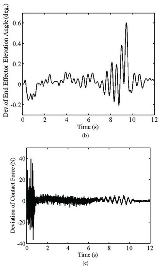
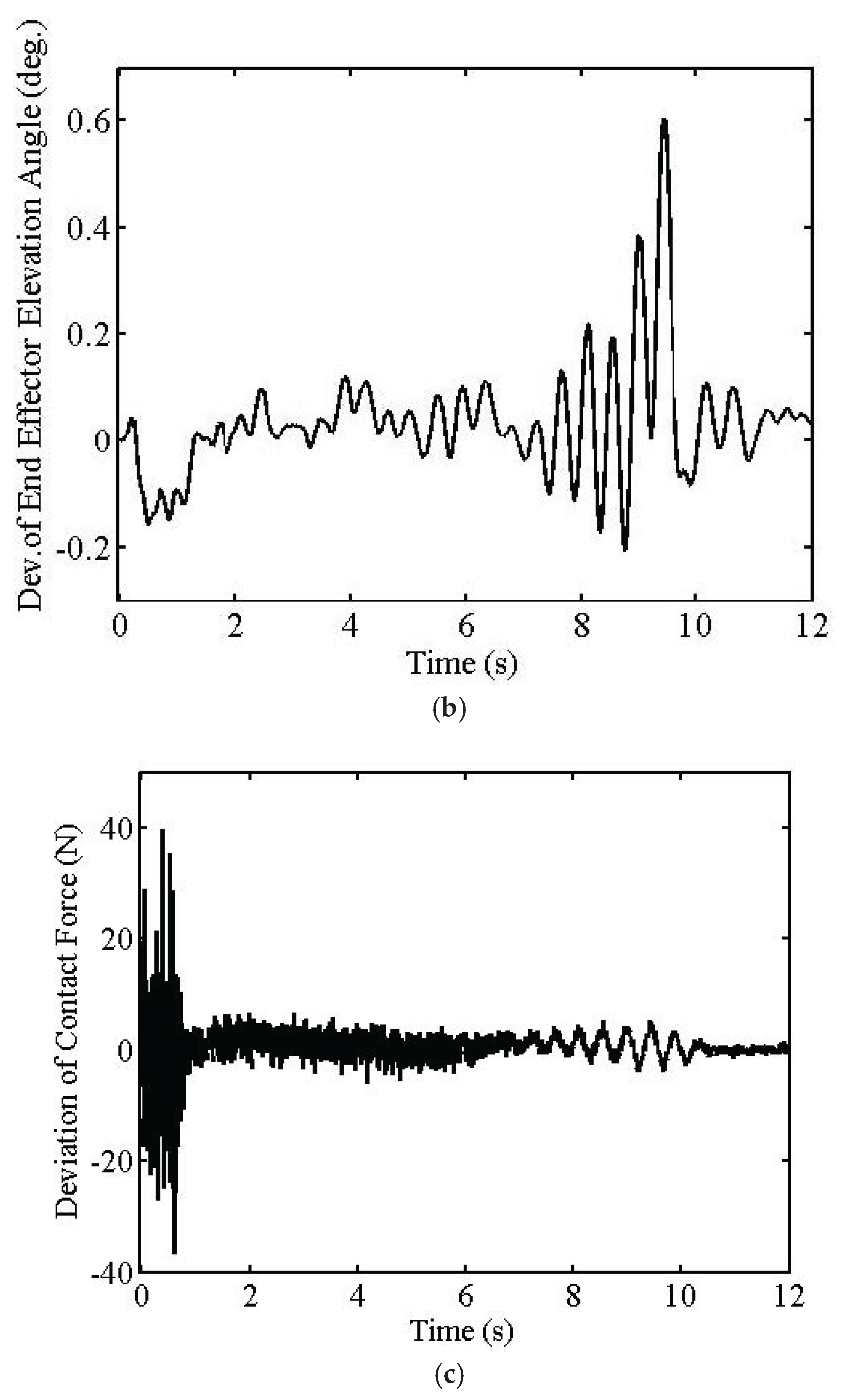
Figure 4.
First simulation results. Deviation of azimuth angle (a), elevation angle (b), and contact force (c) of EE.

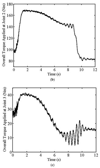
Figure 5.
First simulation results. Joints 1 (a), 2 (b), and 3 (c) torques.
Because of the interference of the dominant CL poles with the smaller crossover frequency (ωc = 150 rad/s), unwanted oscillations are seen in the transient parts of the position and force tracking outputs of the FM, as seen from Figure 3 or Figure 4. However, after the transient part, tracking errors are quite small since the smaller frequency filters the noises more effectively.
By increasing the measurement noise filter crossover frequencies, transient oscillations can be decreased. Therefore, a larger filter crossover frequency (ωc = 250 rad/s) is chosen in the second simulation. This means that the relative stability of the FM is increased by pushing the pole of the filter further away from the dominant CL poles. Therefore, in this case, less noise can be filtered.
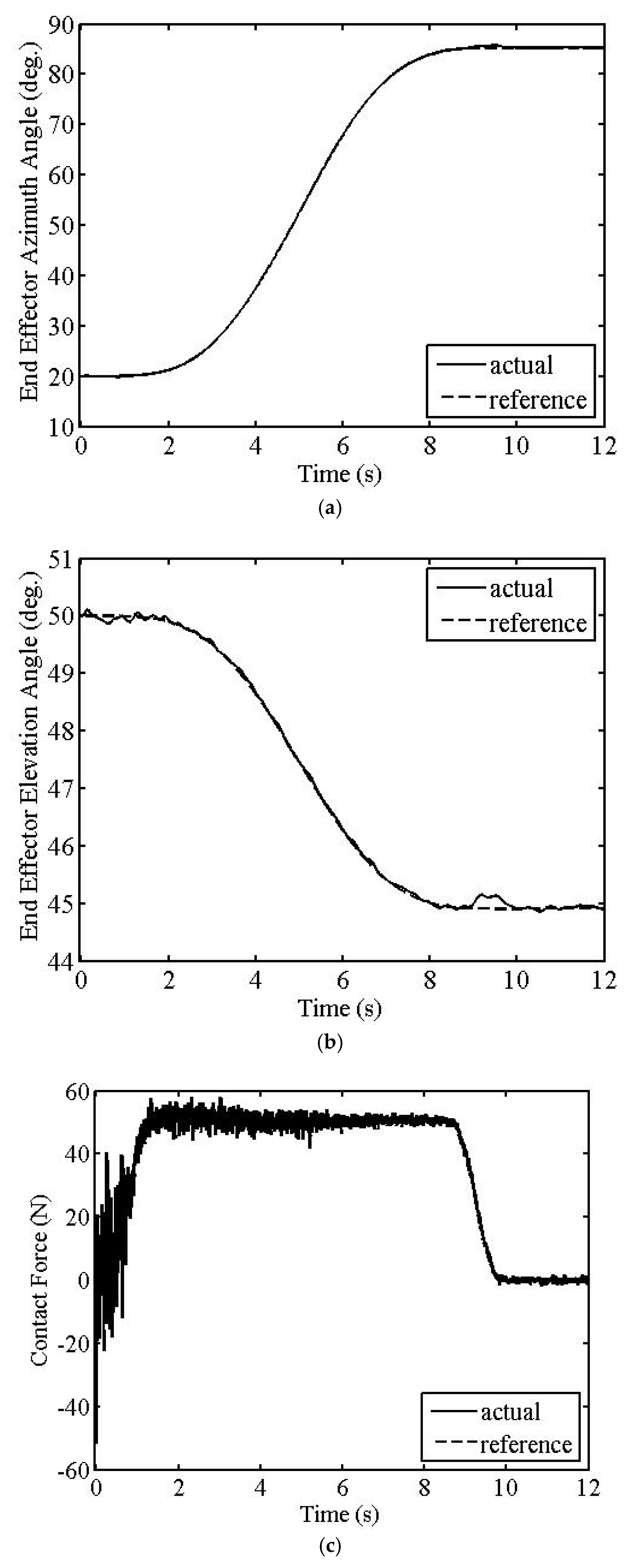
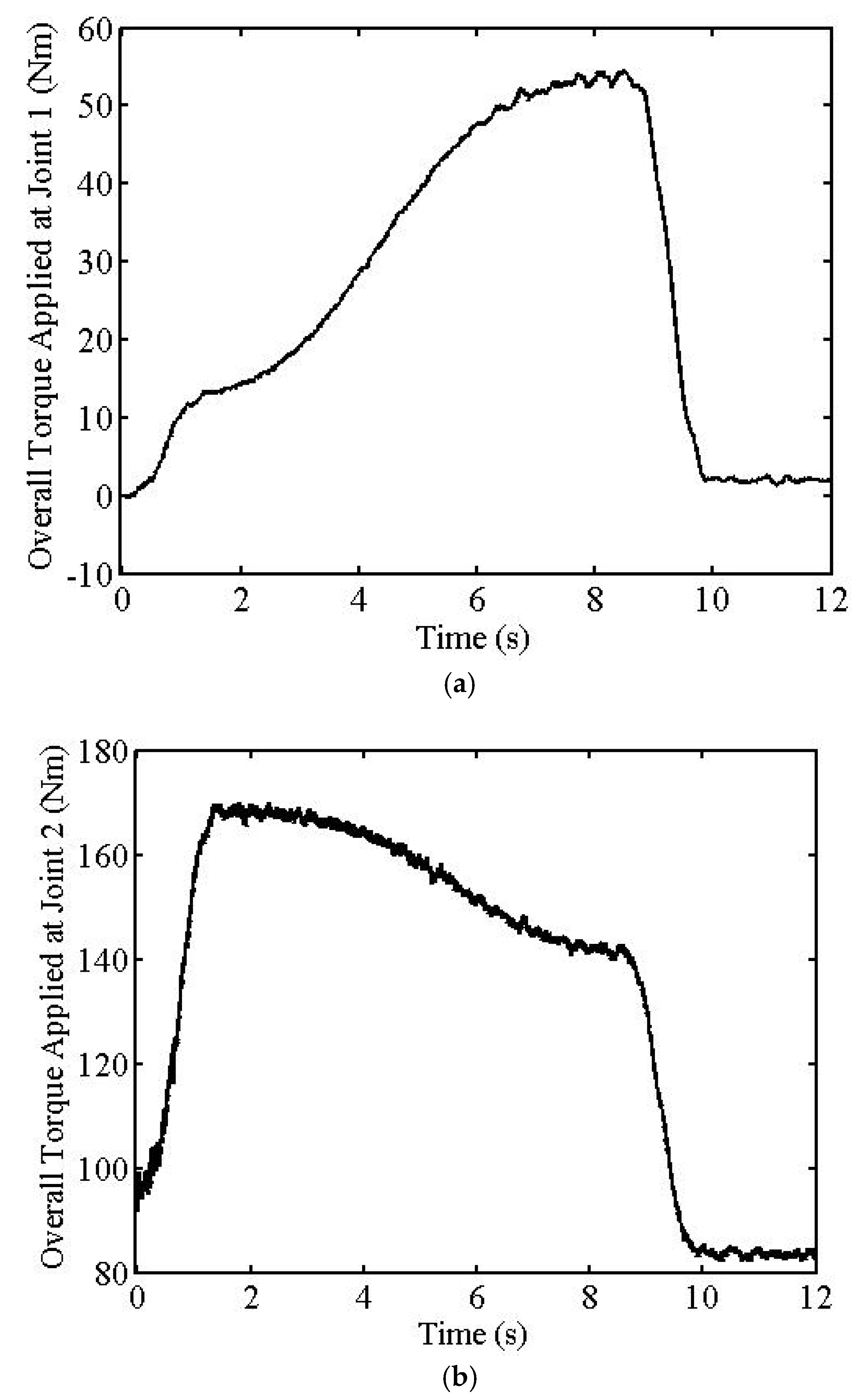
The second simulation results are given in Figure 6, Figure 7 and Figure 8. The maximum tracking error values in the azimuth and elevation angles of the EE are 0.516° and 0.244°, as seen from Figure 6a, Figure 7a and Figure 6b, Figure 7b, respectively. The simulations also show that the maximum contact force error value is 8.083 N after the trajectory is settled, as seen from Figure 6c and Figure 7c. The maximum overall torque values do not exceed 170 Nm, as seen from Figure 8.

Figure 6.
Second simulation results. Azimuth angle (a), elevation angle (b), and contact force (c) of EE.
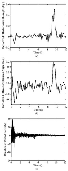
Figure 7.
Second simulation results. Deviation of azimuth angle (a), elevation angle (b), and contact force (c) of EE.
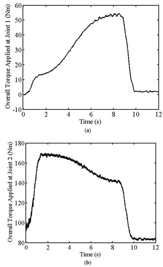

Figure 8.
Second simulation results. Joints 1 (a), 2 (b), and 3 (c) torques.
The position and force tracking transient oscillations are damped out, and trajectory variables settle on the trajectories in a shorter time, as seen from Figure 6 and Figure 7. In addition to this, oscillations of tracking outputs towards the end of the tasks are suppressed. However, towards the end of the task, noise effects are more visible in the tracking outputs.
When the filters’ crossover frequencies are selected as 150 rad/s, unwanted oscillations are seen in the transient parts of the position and force tracking outputs because of the interference of the dominant CL poles with the filters’ crossover frequencies, overall torques are at acceptable magnitudes, and maximum tracking errors are sufficiently small after settling the trajectory. On the other hand, when the filters’ crossover frequencies are selected as 250 rad/s, which is sufficiently far away from the dominant CL poles, transient oscillations of the tracking outputs are decreased, overall torques are at acceptable magnitudes, and maximum tracking errors are sufficiently small after the trajectory is settled. Thus, these two simulations show the effects of the crossover frequency values on the system outputs.
EE position variables may be measured by using optical or proximity sensors. For additional information, encoders may be used for the measurements of the joint variables. EE force and/or moment sensors may be used to measure the contact forces and/or moments. Elastic variables can be obtained by utilizing the measurements of strain gauges. Measurements of strain gauges and joint encoders can be used for the estimations of the EE position variables if the measurements of EE position variables cannot be obtained due to working conditions [25].
7. Conclusions
This work addresses the EE trajectory-tracking FMC of a realistic three-dimensional three-link robot considering measurement noises. The last TLs of the manipulator are considered as structurally flexible. The absolute coordinate approach is used while obtaining the DEs to avoid complex DEs. In this approach, each link is modeled as if there is no connection between the links. After that, constraint equations are written for the connections of the links. Then, these constraint equations are used in DEs to decrease the number of equations. After that, the resulting DEs are transformed into a form which is proper for controller design.
The control method used in this work has many advantages. One advantage is that at the pseudostatic equilibrium, elastic variables and torques can be calculated easily by using algebraic equations. Another advantage is that, though the related matrices are dependent on the position and velocity level variables, there are linear relationships between accelerations and torques. Therefore, by the proper placement of the CL poles, linear control approaches can be applied to reduce deviations from the pseudostatic equilibrium without linearization. So, the system’s non-minimum phase characteristics are managed in this way. As a result of this, this method can be applied easily when compared to methods that need linearization. Particularly, if the DOF of the manipulator is high, this feature of the technique is very beneficial. The third advantage is that, since the EE variables are used as the controlled variables, better tracking accuracy may be obtained when compared to the methods that use joint angular variables as the controlled variables.
In general, overall torques were at acceptable magnitudes and maximum tracking errors were sufficiently small after the trajectory was settled. To filter noises in measured variables, a low pass filter with first-order dynamics was introduced. Filter crossover frequency selection is important to decrease the noise at high frequencies effectively. To demonstrate the effect of crossover frequency on the output, the FMC of the FM was simulated two times using different crossover frequencies for each simulation. Because of the interference of the dominant CL poles with the smaller crossover frequency (ωc = 150 rad/s), unwanted oscillations were seen in the transient parts of the position and force tracking outputs of the FM. However, after the transient part, tracking errors were quite small since the smaller frequency filtered the noises more effectively. By increasing the measurement noise filter crossover frequencies, transient oscillations could be decreased. Therefore, a larger filter crossover frequency (ωc = 250 rad/s) was chosen in the second simulation. This meant that the relative stability of the FM was increased by pushing the poles of the filter further away from the dominant CL poles. This was obtained at the cost of permitting more noise to be filtered in. The position and force tracking transient oscillations were damped out and trajectory variables settled on the trajectories in a shorter time. In addition to this, oscillations of tracking outputs towards the end of the task were suppressed. However, towards the end of the task, noise effects were more visible in the tracking outputs.
Author Contributions
All authors have equally contributed to the conceptualization, methodology, and writing of this research. All authors have read and agreed to the published version of the manuscript.
Funding
This research received no external funding.
Institutional Review Board Statement
Not applicable.
Informed Consent Statement
Not applicable.
Data Availability Statement
Not applicable.
Conflicts of Interest
The authors declare no conflict of interest.
References
- Mosayebi, M.; Ghayour, M.; Sadigh, M.J. A nonlinear high gain observer based input-output control of flexible link manipulator. Mech. Res. Commun. 2012, 45, 34–41. [Google Scholar] [CrossRef]
- Pereira, E.; Trapero, J.R.; Diaz, I.M.; Feliu, V. Adaptive input shaping for single-link flexible manipulators using an algebraic identification. Control Eng. Pract. 2012, 20, 138–147. [Google Scholar] [CrossRef]
- Wang, H.; Kang, S. Adaptive neural command filtered tracking control for flexible robotic manipulator with input dead-zone. IEEE Access 2019, 7, 22675–22683. [Google Scholar] [CrossRef]
- Latip, S.F.A.; Husain, A.R.; Mohamed, Z.; Basri, M.A.M. Adaptive PID actuator fault tolerant control of single-link flexible manipulator. Trans. Inst. Meas. Control. 2019, 41, 1019–1031. [Google Scholar] [CrossRef]
- Zhang, C.; Yang, T.; Sun, N.; Fang, Y. An adaptive fuzzy control method of single-link flexible manipulators with input dead-zones. Int. J. Fuzzy Syst. 2020, 22, 2521–2533. [Google Scholar] [CrossRef]
- Dong, J.; He, B.; Ma, M.; Zhang, C.; Li, G. Open-closed-loop PD iterative learning control corrected with the angular relationship of output vectors for a flexible manipulator. IEEE Access 2019, 7, 167815–167822. [Google Scholar] [CrossRef]
- Cambera, J.C.; Feliu-Batlle, V. Input-state feedback linearization control of a single-link flexible robot arm moving under gravity and joint friction. Robot. Auton. Syst. 2017, 88, 24–36. [Google Scholar] [CrossRef]
- Sun, C.; Gao, H.; He, W.; Yu, Y. Fuzzy neural network control of a flexible robotic manipulator using assumed mode method. IEEE Trans. Neural Netw. Learn. Syst. 2018, 29, 5214–5227. [Google Scholar] [CrossRef]
- Ozguney, O.C.; Burkan, R. Fuzzy-terminal sliding mode control of a flexible link manipulator. Acta Polytech. Hung. 2021, 18, 179–195. [Google Scholar] [CrossRef]
- Qiu, Z.; Wang, B.; Zhang, X.; Han, J. Direct adaptive fuzzy control of a translating piezoelectric Flexible manipulator driven by a pneumatic rodless cylinder. Mech. Syst. Signal Process. 2013, 36, 290–316. [Google Scholar] [CrossRef]
- Abe, A. An effective trajectory planning method for simultaneously suppressing residual vibration and energy consumption of flexible structures. Case Stud. Mech. Syst. Signal Process. 2016, 4, 19–27. [Google Scholar] [CrossRef] [Green Version]
- Forbes, J.R.; Damaren, C.J. Design of optimal strictly positive real controllers using numerical optimization for the control of flexible robotic systems. J. Frankl. Inst. 2011, 348, 2191–2215. [Google Scholar] [CrossRef]
- Qiu, Z.-C.; Li, C.; Zhang, X.-M. Experimental study on active vibration control for a kind of two-link flexible manipulator. Mech. Syst. Signal Process. 2019, 118, 623–644. [Google Scholar] [CrossRef]
- Zhang, S.; Zhang, Y.; Zhang, X.; Dong, G. Fuzzy PID control of a two-link flexible manipulator. J. Vibroeng. 2016, 18, 250–266. [Google Scholar]
- Khan, M.U.; Kara, T. Adaptive control of a two-link flexible manipulator using a type-2 neural fuzzy system. Arab. J. Sci. Eng. 2020, 45, 1949–1960. [Google Scholar] [CrossRef]
- Pradhan, S.K.; Subudhi, B. Position control of a flexible manipulator using a new nonlinear self-tuning PID controller. IEEE/CAA J. Autom. Sin. 2020, 7, 136–149. [Google Scholar] [CrossRef]
- Pedro, J.O.; Smith, R.V. Real-time hybrid PID/ILC control of two-link flexible manipulators. IFAC Pap. 2017, 50, 145–150. [Google Scholar] [CrossRef]
- Yang, X.; Zhong, Z. Dynamics and terminal sliding mode control of two-link flexible manipulators with noncollocated feedback. In Proceedings of the 3rd IFAC International Conference on Intelligent Control and Automation Science, Chengdu, China, 2–4 September 2013; pp. 218–223. [Google Scholar]
- Wang, Y.; Niu, Z.; Yang, M.; Xu, Q. Decoupled terminal sliding mode control of two link flexible manipulators with motor dynamics. In Proceedings of the IECON 2019—45th Annual Conference of the IEEE Industrial Electronics Society, Lisbon, Portugal, 14–17 October 2019; pp. 336–340. [Google Scholar]
- Rahmani, B.; Belkheiri, M. Adaptive neural network output feedback control for flexible multi-link robotic manipulators. Int. J. Control 2019, 92, 2324–2338. [Google Scholar] [CrossRef]
- Xu, B. Composite learning control of flexible-link manipulator using NN and DOB. IEEE Trans. Syst. Man Cybern. Syst. 2018, 48, 1979–1985. [Google Scholar] [CrossRef]
- Shafei, H.R.; Bahrami, M.; Talebi, H.A. Design of adaptive optimal robust control for two-flexible-link manipulators in the presence of matched uncertainties. J. Vib. Control 2021, 27, 612–628. [Google Scholar] [CrossRef]
- Kilicaslan, S.; Ider, S.K.; Özgören, M.K. Motion control of a spatial elastic manipulator in the presence of measurement noises. Arab. J. Sci. Eng. 2021, 46, 12331–12354. [Google Scholar] [CrossRef]
- Kilicaslan, S.; Özgören, M.K.; Ider, S.K. Hybrid force and motion control of robots with flexible links. Mech. Mach. Theory 2010, 45, 91–105. [Google Scholar] [CrossRef]
- Kilicaslan, S. Unconstrained Motion and Constrained Force and Motion Control of Robots with Flexible Links. Ph.D. Dissertation, Department of Mechanical Engineering, Middle East Technical University, Ankara, Turkey, 2005; 412p. [Google Scholar]


Publisher’s Note: MDPI stays neutral with regard to jurisdictional claims in published maps and institutional affiliations. |
© 2022 by the authors. Licensee MDPI, Basel, Switzerland. This article is an open access article distributed under the terms and conditions of the Creative Commons Attribution (CC BY) license (https://creativecommons.org/licenses/by/4.0/).