Abstract
The service conditions of underground coal mine equipment are poor, and it is difficult to accurately extract the fault characteristics of rolling bearings. In order to better improve the accuracy of the fault identification of rolling bearings, a fault-detection method based on multiscale permutation entropy and SOA-SVM is proposed. First, the whale optimization algorithm is used to select the modal analysis number K and the penalty factor α of the variational mode decomposition algorithm. Then, the vibration signal of rolling bearings is dissolved according to the optimized variational mode decomposition algorithm, and the multi-scale permutation entropy of the main intrinsic mode function is calculated. Finally, the feature values of the matrix are entered into the SVM algorithm optimized by the seagull optimization algorithm to obtain the classification result. The experimental results based on the published rolling bearing datasets of Western Reserve University show that the identification success rate of the proposed method can reach 98.75%. The fault detection of the rolling bearings can be completed accurately and efficiently.
1. Introduction
As a key component of rotating machinery and equipment, the operating conditions of rolling bearings immediately impact the working characteristics of mining fans. When there is a problem with a rolling bearing, the damage point constantly collides with other parts that it touches, resulting in shock oscillation and unstable, nonlinear, multi-frequency data signals [1]. Sudden faults such as loose or damaged rolling bearings will cause uneven bearing capacity, the expansion of frictional resistance, or shutdown, leading to faults such as displacement, unbalance, and the surge of the mining fan. The problems caused by rolling bearings account for about 50% of the common failures of mining fans, and the shutdown time caused by rolling bearings also accounts for about 45%. Therefore, the accurate identification of faults of rolling bearings is of key practical significance to the safety and stability of mining fans.
The stucture of rolling bearing determines the load distribution showing cycling changes. Rolling balls and outer race cantact point changes will make the stiffness of the system form a periodic change, thus producing harmonic vibration. The causes of vibration include raceway waviness, radial play, ball errors, etc. Zmarzły [2] evaluates the impact of the race’s roundness and waviness deviations, radial clearance, and total curvature ratio on the vibration. Vibration will occur whether the rolling bearing is normal or not. Different vibration characteristics of the bearing can reflect the different operating conditions of the bearing. The testing of rolling bearing vibration can be classified into three groups. The first group concerns the evaluation of the vibration of new rolling bearings on testing rigs. The second testing group concerns the vibration analysis of rolling bearings operating in real application conditions. The third testing group concerns the intentional induction of defects or damage in rolling bearing elements to determine their impact on the generated vibration.
Vibration analysis method is widely used in rolling bearing fault diagnosis because it reveals the inherent characteristics of the bearing fault [3]. Generally speaking, the reliability analysis method mainly includes three levels: data preprocessing, fault feature extraction, and failure mode classification [4]. Because the evaluation of vibration signal usually shows the characteristics of optimal control and instability, the research in recent years is mainly concentrated on time-frequency analysis technology [5]. At present, there are two types of time-frequency analysis technology. The first methods do not need to establish the primary parameters before examining the vibration signals. A very typical example is empirical mode decomposition (EMD) [6]. EMD is a responsive reliability analysis technology, which can dissolve all complicated data signals into several characteristic modal analysis function formulas according to the original vibration. Although several applications have proved the efficiency of EMD in detecting rolling bearing faults [7], it still has issues with the terminal effect and modal aliasing. The second methods need to set some main parameters before they are used to analyze vibration signals, such as wavelet transform (WT). However, this method must define the wavelet basis function and threshold in advance [8], and the choice of wavelet basis function has a considerable influence on the final output. Therefore, the wavelet transform does not have adaptive characteristics.
Dragomiretshiy [9] introduced variational mode decomposition (VMD) as a method for determining the frequency center and the bandwidth of a variational model. Compared with empirical mode decomposition and wavelet transform, variational mode decomposition has a rigorous mathematical theoretical foundation and can separate vibration signals efficiently and accurately. Although the frequencies of the vibration signals can be adaptively divided by the VMD method, the attenuation results are still limited by the choice of the modal number K and the penalty parameter α. Z. Zhang [10] determined the selection of K value by observing the center frequency of intrinsic mode function (IMF). Z. Guo [11] selected the appropriate number of decomposition layers by setting the threshold of multi-scale permutation entropy. With the increasing applications of intelligent algorithms, researchers tend to combine intelligent algorithms with parameter optimization of VMD. G. A. Ran [12] introduced the grey wolf algorithm to optimize K. J. Li [13] introduced genetic algorithm to optimize K and α at the same time. Although it takes a very long time to optimize the parameters of variational mode decomposition with intelligent algorithm, it has become a research hotspot because it considers the coupling impact of the two factors on the decomposition effect.
Following the dissolution of the vibration data signal into a sequence of IMFs via VMD, the next task is how to obtain the fault information from the obtained IMF weights. Richman explicitly proposed the sample entropy [14]. Because sample entropy is less sensitive to data length and noise, it is of general concern. Permutation entropy (PE) was suggested by Bandt [15] to analyze the plurality of mechanical systems and assess their conditions. Since PE considers complexity in terms of relatively close proximity, it is simple and not compromised by noise. However, sample entropy and permutation entropy estimate complexity only on a single scale, which will produce adverse results when applied to the analysis of data on multiple time scales. In view of this shortcoming, Costa [16] developed a method for assessing the complexity of unprocessed time series at different scales using a multi-scale sample entropy approach. However, the complexity estimation of the actually measured bearing fault vibration signal by multi-scale sample entropy is poor, and the processing of a long time series is particularly time-consuming. To assess the complexity of time-series data, Aziz and ARIF [17] introduced the multiscale permutation entropy (MPE). In addition, the stability and robustness of MPE were verified. J. Zheng [18] employed MPE and SVM to identify rolling bearing defects, proving the superiority of MPE in the feature extraction of rolling bearing faults. Therefore, MPE is selected as a special tool for the SVM algorithm in this paper.
At this stage, the specific methods used for rolling bearing fault classification include SVM [19], the extreme learning machine [20], the BP neural network [21], etc. In small samples, SVM has strong generalization ability and a relatively simple structure. The SVM solid model has two key main parameters C and g, where C is the penalty index, the tolerance for deviation. If the C value is too large, it is easy to achieve multicollinearity; and if the C value is too small, it is easy to underfit. If C is too large or too small, it will lead to the poor generalization ability of SVM [22]. g is the main parameter after the RBF function formula is evaluated as a kernel function. It categorizes the data after projecting it explicitly to the interior space with new features. The larger the g value is, the less applicable the space vectors are; and the smaller the g value is, the more applicable space vectors are. The number of applicable space vectors can compromise the rate of training. The intelligent optimization algorithm is often used to select C and g of the support vector machine. J. Zheng [23] optimized SVM for rolling bearing defect type detection using the cuckoo search method, and its overall recognition rate reached 98.03%.
Inspired by previous scientific research, a combined model based on multi-scale permutation entropy and SOA-SVM is pointed out in this paper. First, the envelope entropy is adopted as the fitness function of the whale optimization algorithm to obtain the preset parameter pair of the variational mode decomposition algorithm [K, α]. Then, the bearing vibration signal is decomposed by using the variational mode decomposition algorithm optimization of the parameters to generate a set of intrinsic mode functions. The multi-scale permutation entropy of the main intrinsic mode functions is calculated on the basis of the kurtosis and correlation coefficient to form the feature vector. Finally, the SOA-SVM method is employed to identify four statuses of rolling bearing (normal, inner ring fault, outer ring fault, and rolling element fault).
2. The Proposed Method
2.1. WOA-VMD
VMD has a high signal attenuation efficiency as a prominent time-frequency analysis approach [24]. For the original signal x(t), it can be decomposed into a series of intrinsic mode functions IMFs ui in automation mode.
To guarantee the minimum sum of the bandwidth of each center frequency, the process can be expressed as
where = {u1,…ui} is a series of decomposed intrinsic mode functions, and {ωk} = {ω1,…ωk} is the center frequency corresponding to each intrinsic mode function. In order to arrive at the best solution in Equation (2), the Lagrange penalty factor L and secondary penalty factor α are introduced.
The combination of decomposition levels K and the penalty factor α has a significant impact on the decomposition result of the variational mode decomposition method [25]. Over-decomposition, and erroneous components, will result if the K value is too high; under-decomposition will result if the K value is too low. The bandwidth surrounding each center frequency will be too narrow if the value is too high. The bandwidth surrounding each center frequency will be too wide if the value is too low. Improper parameter selection will lead to the difficulty of subsequent feature extraction, which will affect the final accuracy of the fault recognition. Therefore, the reasonable parameter setting is very important to get satisfactory decomposition results.
WOA was explicitly proposed by Mirjalili [26] based on the scientific research on the hunting behavior of whales. WOA is selected because this method has the advantages of fast improvement speed, strong global convergence, and a few parameters. The specific steps of the WOA optimization are as follows:
- (1)
- The initialization of parameters such as whale individual population, location, and iteration times. The i-th individual location is:where is a random number within the range of [0, 1]. is in the range of [, ]. is the minimum value of the parameter boundary, and is the maximum value of the parameter boundary.
- (2)
- When p < 0.5 and |A| < 1, shrink and surround according to the best search agent, as shown in Equation (5):where , , and p are random numbers, and the value range is [0, 1]. i is the current number of iterations; is the maximum number of iterations.
When p < 0.5 and |A| ≥ 1, a random search agent is selected to iterate and update the Expression (6). is the whale position vector selected randomly.
When p ≥ 0.5, the spiral contraction method is adopted for iteration, as shown in Formula (7):
where is the distance between simulated whales and prey; b is the defined helix constant; and m is a random number between (−1, 1).
- (3)
- Check if the termination requirements have been satisfied or if the maximum number of repetitions has been reached. If not, return to step (2). If yes, output the best search agent.
Using the whale optimization algorithm, it is also necessary to select the appropriate fitness function [27]. In this paper, the envelope entropy proposed by Tang Guiji [28] is used as the fitness function, and its expression is as follows:
where is a sequence of probability distribution processed by the envelope signal; is the envelope signal got by Hilbert Demodulation of the original signal [29]; and is envelope entropy, which can quantitatively measure the sparsity of vibration signals [30].
When the signal contains a large number of interference components, the fault impact and modulation phenomenon caused by the fault will be hidden in the signal, resulting in the weakening of the sparsity of the signal, and the envelope entropy value is large at this time. The sparsity of the signal is high, and the envelope entropy value is low when it contains clear fault impact and modulation events. The envelope entropy is used as the fitness function for the parameter optimization of VMD, and its minimum is taken as the search goal of the algorithm to complete the optimization of relevant parameters.
The process of optimizing VMD parameters with WOA is shown in Figure 1. First, initialize the whale group position vector [K, α]. The fitness function is the envelope entropy, and each whale’s fitness is evaluated. Then, by judging the size of the convergence factor, the iterative formula is selected for iterative update until the termination conditions are met, and the optimal VMD parameters are output. The upper boundary of the whale group position is set to [10, 3000]; the lower boundary is set to [3, 300]. The convergence criterion is 10, and the population number is set at 20.
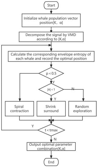
Figure 1.
A flowchart of the WOA-optimizing VMD parameters.
2.2. Multiscale Permutation Entropy and Its Parameter Setting
The related concepts of multi-scale permutation entropy are shown in reference [31], and its theory is described as follows.
The original time series with length n is coarsened to obtain a new time series:
where s is the scale factor and s = 1, 2, …; indicates rounding. Each scale sequence’s time reconstruction of each scale sequence is as follows:
The reconstructed sequences are placed in order if their values are same. A collection of symbol sequences can be produced for every scale sequence, where r = 1, 2, 3, …, R and R ≤ m!. One of the permutations is the symbol sequence , and the chance of each symbol sequence occurring is determined (r = 1, 2, …, R). Information entropy is used to define the permutation entropy of various symbol sequences.
When = , the maximum value is reached. For convenience, normalization is usually performed.
Four parameters must be established before MPE can be used: time-series length N, encapsulation dimension m, scale factor s, and time delay . Because m is the number that specifies the maximum number of permutations m!, permutation entropy depends largely on the choice of encapsulation dimension m. In addition, the length of time series N should be more than 5 * m factorial [32] to obtain reliable statistics. Bandt [15] pointed out that this method is suitable for the case where the encapsulation dimension is 3 ≤ m ≤ 7. The approach will not function if the encapsulation dimension m is too small since there are too few different states. When the encapsulation dimension m is too large, on the other hand, it will be too time-consuming. Typically, the encapsulation dimension m is chosen based on balancing information content impairment and measurement complexity. m is set to 5 in this article. We put = 1 here since the time delay has no significant impact on the outcome. The calculation efficiency is jeopardized when N is too high. The criterion of N ≥ 5 m! cannot be met if N is too small. Taking this control into account, the data length of 2048 points is sufficient to get a stable permutation entropy. Therefore, N is set to 2048. The scale factor s is set to 15 to obtain the permutation entropy of each scale. Finally, we put = 1 here since the time delay has no significant impact on the outcome.
2.3. SOA-SVM
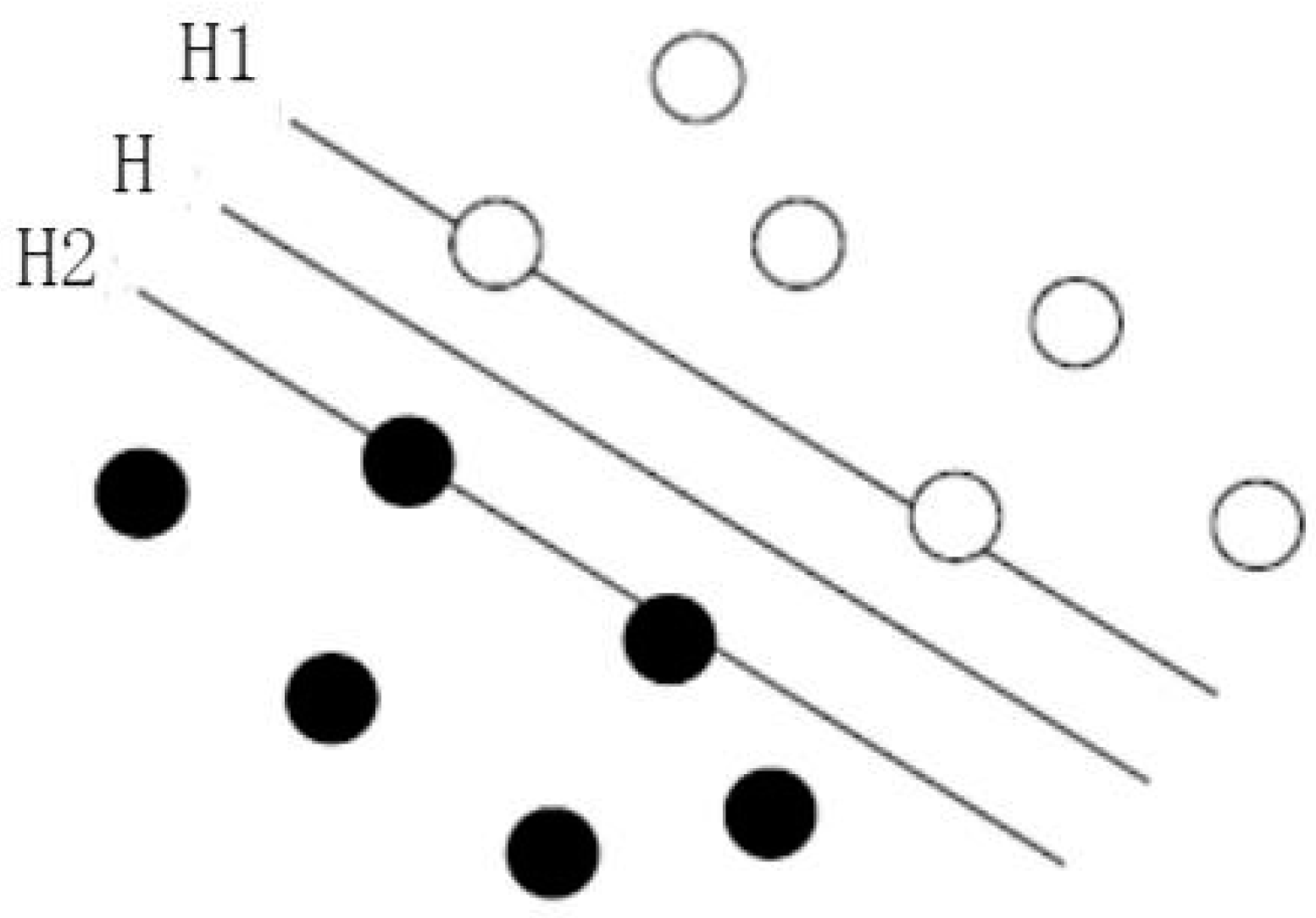
The support vector machine (SVM) was proposed in the early 1990s. It is based on the statistical learning theory’s VC measure idea and the structural risk reduction principle. It can balance the amount of computation and the ability of computation on the basis of limited sample information. Its superior data classification and recognition ability makes it very effective in rolling bearing fault diagnosis. The population classification in the case of linear separability is shown in Figure 2. It can be seen from the figure that two different types of samples are divided by the optimal hyperplane H, and the purpose of SVM classifier is to find the hyperplane.

Figure 2.
The optimal hyperplane diagram.
Let the two types of sample sets in the graph be ; n is the number of samples, and xi is the ith input value of the sample feature space. In the linearly separable state, the optimal hyperplane solved by the support vector classifier can be transformed into the following constraint problem:
where is the normal vector of the hyperplane; m is the offset; = 0 is the hyperplane to be solved.
If the nature of the sample is linearly inseparable, the support vector machine will map the sample from the current space to the high-dimensional space Λ using nonlinear mapping Ψ. In this way, the problem of linear inseparability can be transformed into linear separability. Therefore, the optimal hyperplane can be obtained on the high-dimensional space Λ, but the kernel function k(xi, xj) must meet the positive definite matrix condition, that is,
By selecting the appropriate kernel function k(xi,xj), the nonlinear samples can be linearized and classified. After the relaxation variable ξi is introduced, the expression of the original classification hyperplane is
where C is the penalty factor. After introducing the Laplace multiplication operator, the optimal classification hyperplane problem is transformed into a dual quadratic programming problem. At the same time, it is substituted into the inner product transformation of the kernel function, and Formula (15) becomes
The final classification hyperplane can be expressed as
The parameter setting of the support vector machine algorithm affects its learning and generalization ability, so knowing how to select the optimal parameters has great research value. When k(xi, xj) is the radial basis function, the debugging of penalty factor C and kernel width g is the major focus of SVM parameter adjustment.
Gaurav Dhiman [33] introduced the Seagull optimization algorithm (SOA) as a new swarm intelligence optimization technique in 2018. The algorithm mainly simulates the migration behavior and the attack behavior of seagull groups in nature. Migration refers to the movement of seagulls from one position to another, while seagulls should meet three conditions: avoiding collision, the direction of the best position direction, and the approaching of the best position [34].
- (1)
- Avoid collision. In order to prevent the occurrence of a collision between adjacent seagulls, add a new variable a. The formula is:where represents the new position of seagulls after collision avoidance; indicates the current number of iterations; indicates the initial position of the seagull; and represents the motion behavior of seagulls in a given search space. The calculation formula of is:where the value of A is adjusted by f linearly, and it decreases linearly from to 0; is the maximum number of iterations.
- (2)
- The direction of the best position. On the premise of not colliding with other individuals, seagulls will move in the direction of the best position. The formula iswhere indicates the direction of the best position of the seagull and is mainly responsible for balancing global search and local search. In order to obtain an appropriate balance number, the calculation formula of iswhere is a random number between [0, 1].
- (3)
- Approaching the best position. The seagull will soar in the route of the best position to achieve a new one after landing in a safe location away from other seagulls.where indicates the new position where the seagull meets three conditions.
During migration, seagulls can constantly change the angle and speed of attack. With the help of gravity and wings, they can maintain a certain height in the air. When seagulls attack their prey, they move spirally in the air, and their motion behavior is represented by a, b, and c components, respectively. The formulas of motion behavior are as follows:
where r is the spiral radius in the movement of seagulls; u and v are the correlation constants of spiral shape; θ represents the angle, which is a random number between [0, 2π]; and the formula of seagull’s attack behavior obtained from the movement behavior is
where Zbest(t) indicates the best seagull position. The steps of optimizing support vector machine with seagull algorithm are as follows:
- (1)
- Initialize the population parameters of seagull optimization algorithm, the number of iterations, and the value range of C and g.
- (2)
- Determine the fitness function of seagull optimization algorithm and evaluate the adaptability of seagull individuals on the basis of the value of fitness function. According to the principle of seagull optimization algorithm, find the optimal fitness value and the optimal position obtained by seagull.
- (3)
- According to the best individual position of seagull, the optimal values of parameters C and g are obtained.
- (4)
- The optimal parameters C and g are assigned to the support vector machine for training, and the optimized support vector machine classification model is obtained.
- (5)
- Input the test samples, then the optimized SVM classification model will output the predicted labels of the test samples and compare the predicted labels with the actual labels to obtain the classification accuracy.
3. Experiment and Results
3.1. Experimental System
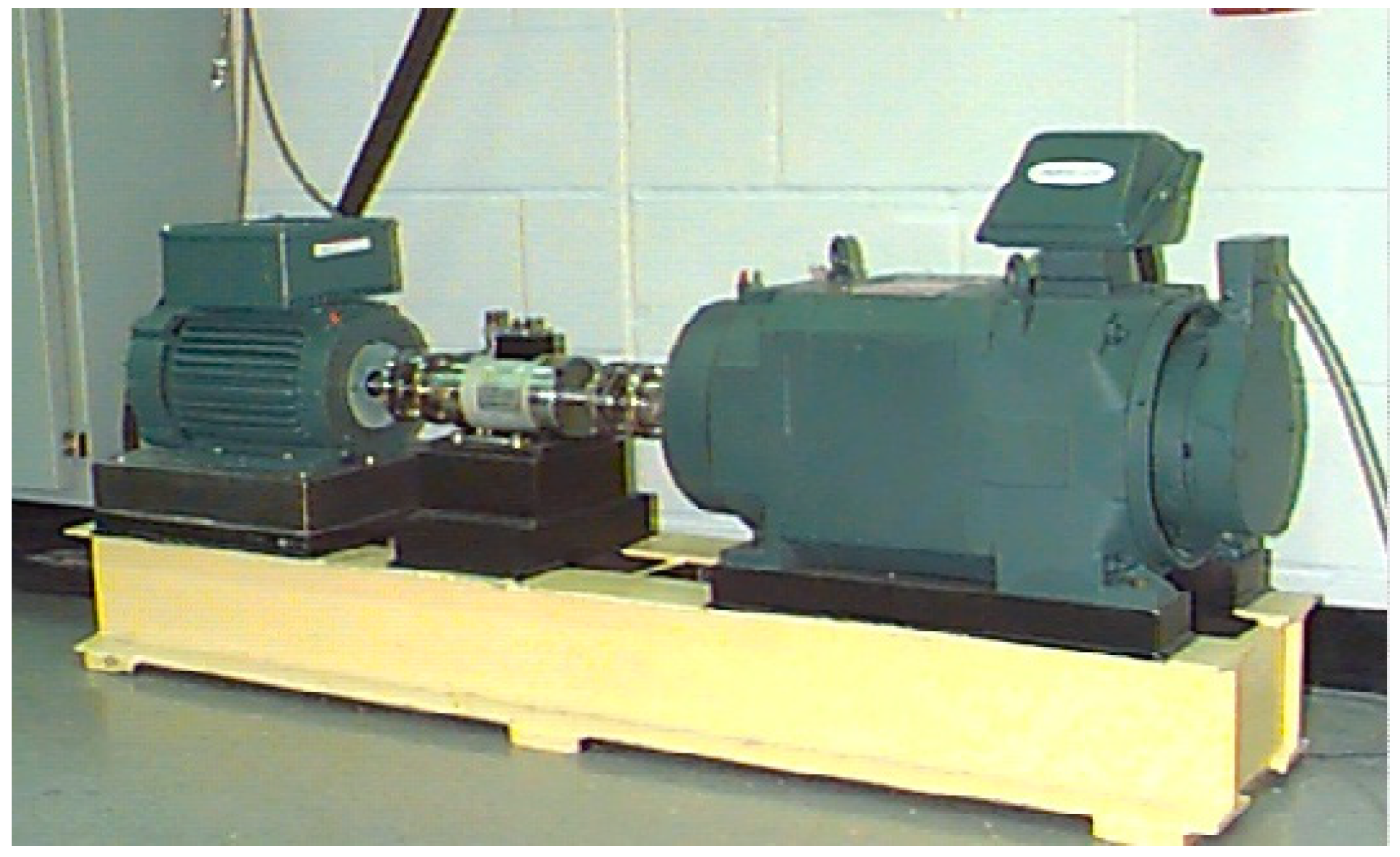
For analysis, select Case Western Reserve University (CWRU) rolling bearing data information. The selected data material is the mechanical vibration data signal of the SKF6205 rolling bearing on the motor drive side. Rolling bearing bore, outside and turning body are wire by EDM 0.007 diameter. The push motor is rated at 1797 rpm. The sampling rate is 12kHz. Figure 3 depicts the structure of the test service platform. When a roller bearing is damaged, the roller bearing can come into contact with failure locations, causing significant shock vibrations. The cycle time for the flip body to touch the common fault location varies by common fault type.
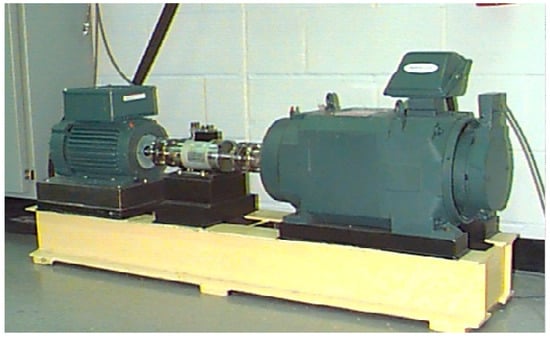
Figure 3.
The data set experiment platform of CWRU.
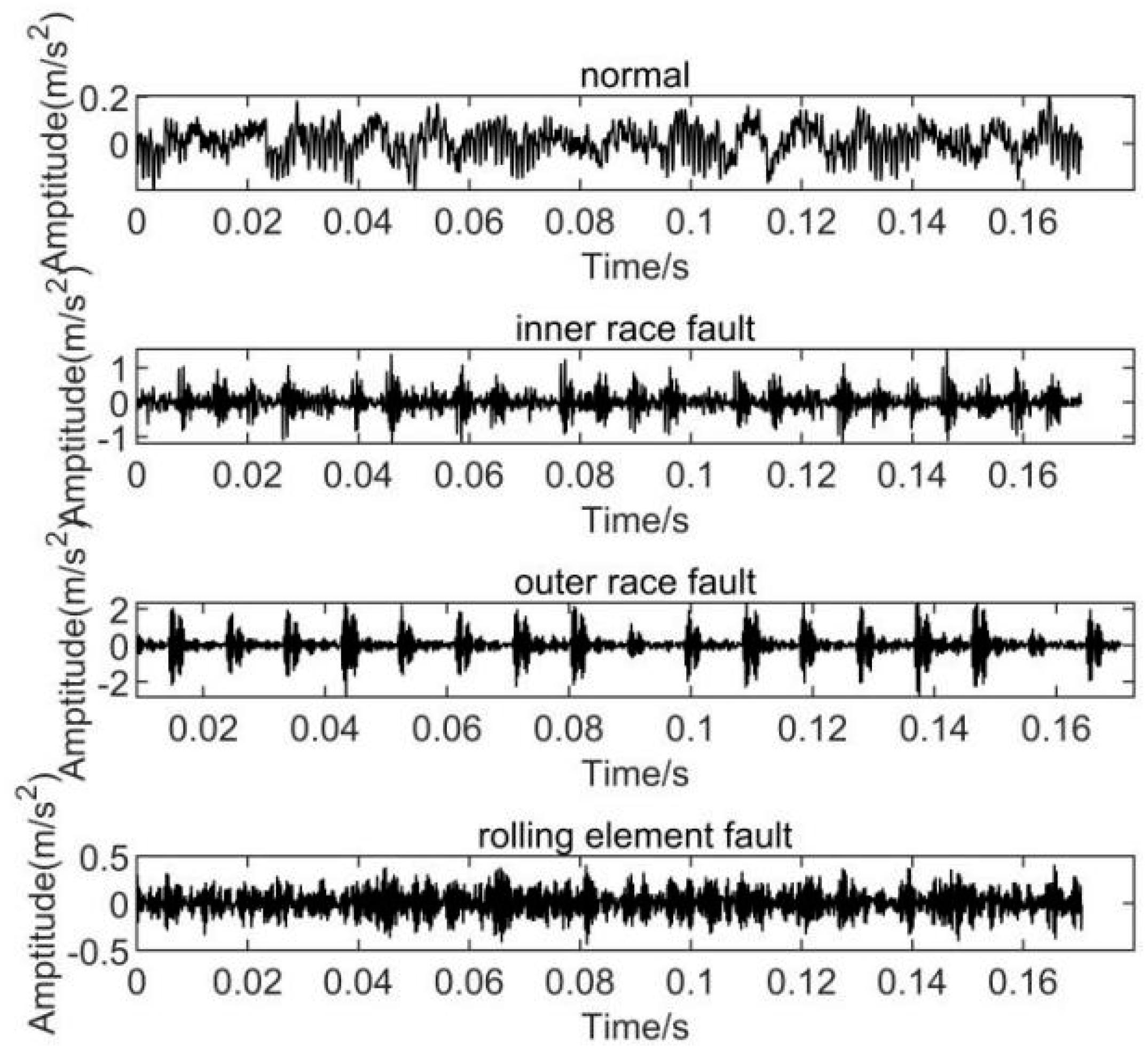
There are four different sorts of flaws that are investigated. Figure 4 shows the different parts of the rolling bearing failures. Figure 5 shows the frequency domain waveforms of the vibration data signals for the four rolling bearing cases. Each type of fault is represented by 50 data groups, 30 of which are training samples in a known state and the remaining 20 are diagnostic test samples. Each batch of vibration data has a sample length of 2048. The sample data set is shown in Table 1.
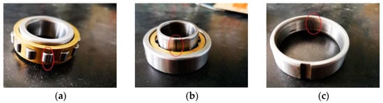
Figure 4.
The different defects of rolling bearings: (a) rolling balls, (b) inner race, and (c) outer race.
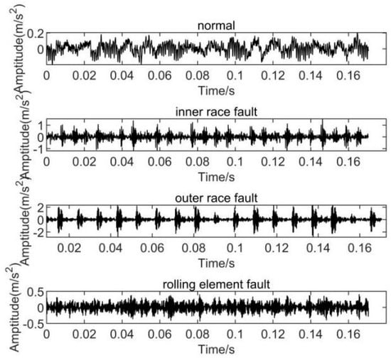
Figure 5.
The time domain waveforms of vibration signals under four bearing states.

Table 1.
A description of the bearing dataset.
3.2. Results and Discussion
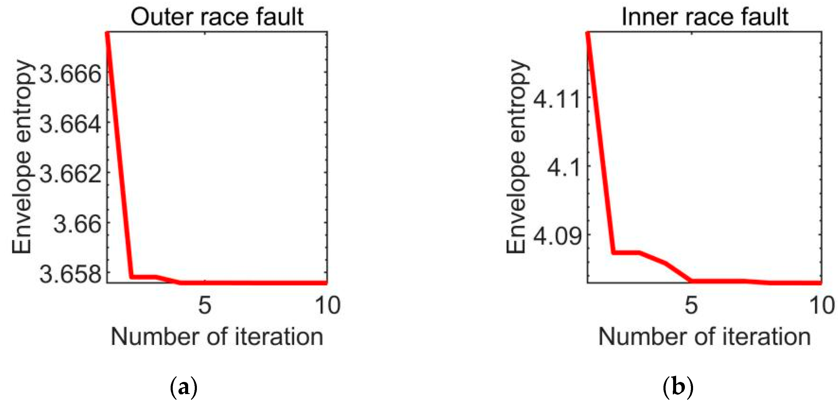
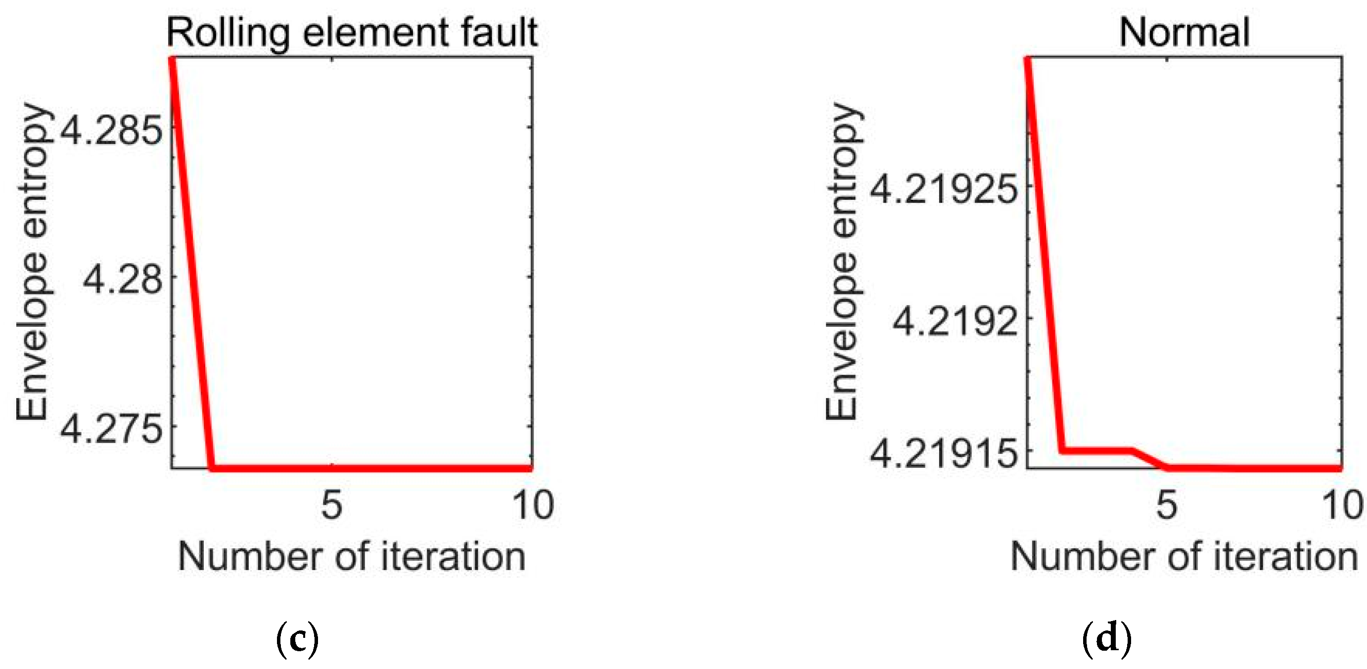
The vibration signal is decomposed using the enhanced VMD method. Taking the outer ring defect as an example, the whale algorithm is utilized to improve the parameters of the VMD algorithm. Figure 6 shows the minimal envelope entropy fluctuation as the number of generations in the WOA optimization process grows. The minimum envelope entropy in the fourth iteration is 3.6576, as seen in the figure. The optimization procedure is complete when the number of iterations hits 10, and the optimization parameters [K, α] are [10, 1469]. The best parameters in Table 2 are used to set the VMD algorithm parameters. Then, the optimized VMD algorithm is used to decompose the vibration signals of different damage positions and degrees of rolling bearing.
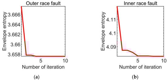
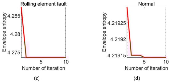
Figure 6.
The optimized VMD curve with WOA.
Table 2.
The optimization parameters obtained by using the WOA.
In the VMD approach, the measurement index is a crucial factor that decides if the decomposition result is satisfactory. In mechanical fault identification, kurtosis is an important index of vibration signal analysis. Kurtosis is a numerical statistic that depicts the features of random variables’ distribution. The kurtosis value is calculated as shown in Equation (28):
where m is the average value of signal x and σ is the standard deviation of signal x. The larger the kurtosis value, the more fault information is contained in the intrinsic mode function. Because kurtosis has nothing to do with factors such as bearing rotation speed, size, and mechanical load and is very sensitive to impact signal, it is particularly suitable to study surface damage faults [35].
The main IMFs after vibration signal decomposition are selected according to kurtosis. According to Table 3, it can be seen that the kurtosis value when modes n = 3, 9, and 10 is always the larger of the 10 modes when different outer ring fault samples are analyzed and calculated; According to Table 4, by analyzing the kurtosis values of different modal components in the inner ring fault with the same method, it can be seen that the kurtosis values of the corresponding modal components in this state when n = 3, 6, and 10 are the larger three; According to Table 5, when n = 3, 4, and 10, the kurtosis value of the corresponding modal component is the larger in the rolling element fault. However, through the analysis of bearing signals under normal conditions, the results shown in Table 6 are obtained, and the kurtosis value of each intrinsic mode function has no obvious law. The reason for this result may be that the definition of kurtosis criterion makes the vibration data in normal state not suitable for kurtosis criterion analysis. According to the correlation coefficient [36] between each intrinsic mode function and the original signal, the modal component n equal to 1, 2, and 4 is selected as the main intrinsic mode function in the normal state for subsequent analysis according to Table 7.
Table 3.
The kurtosis value of each mode of the outer ring fault.
Table 4.
The kurtosis value of each mode of the inner ring fault.
Table 5.
The kurtosis value of each mode of the rolling element fault.
Table 6.
The kurtosis value of each mode of normal.
Table 7.
The correlation coefficient of each mode of normal.
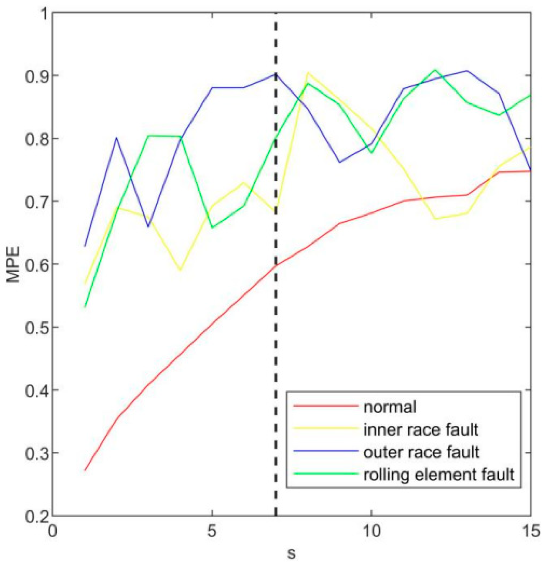
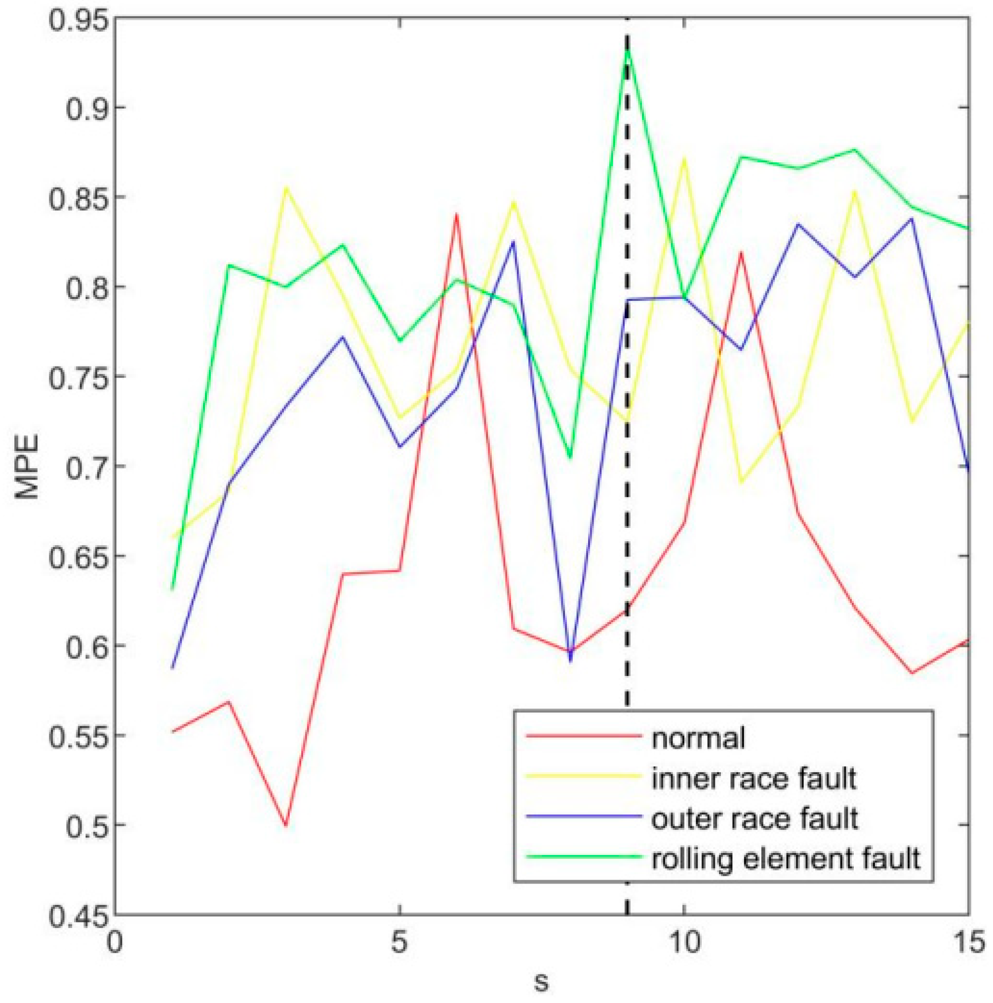
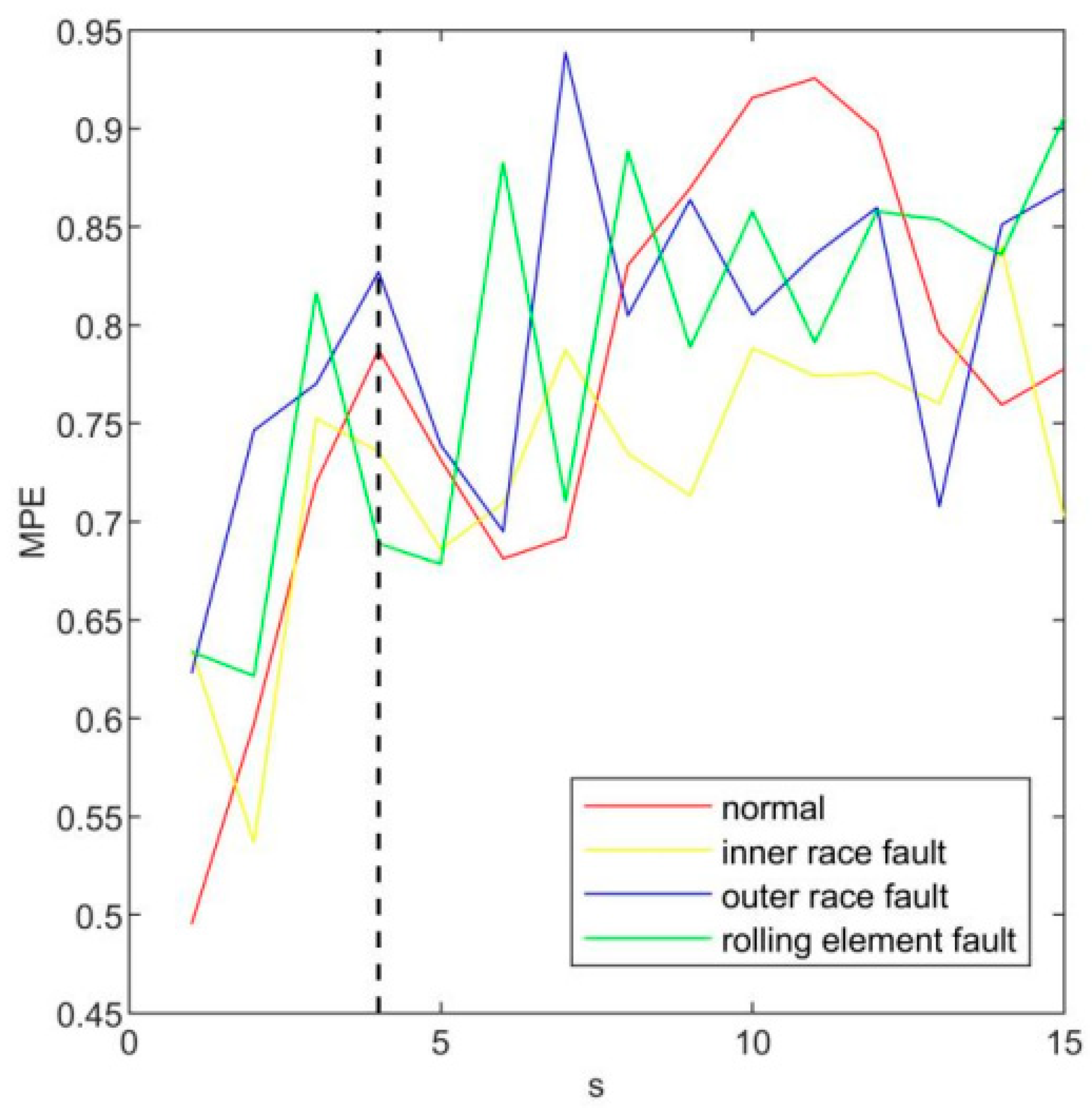
The MPE of three main intrinsic mode functions in four states is calculated, respectively. According to the results shown in Figure 7, when s = 1,2, the permutation entropy calculated by rolling element fault and inner ring fault is very close; when s = 3, the permutation entropy calculated by the inner ring fault and the outer ring fault is very close. If the feature vector is constructed based on these, it may cause the disorder of later state classification. Considering the average distance and minimum distance of the entropy of imf1 multi-scale arrangement in four states, the value of the optimal scale factor s of imf1 is chosen to be 7. Using the same method, the optimal scale factor s of imf2 is 9 and the optimal scale factor s of imf3 is 4 according to the results shown in Figure 8 and Figure 9.

Figure 7.
The MPE of imf1.

Figure 8.
The MPE of imf2.
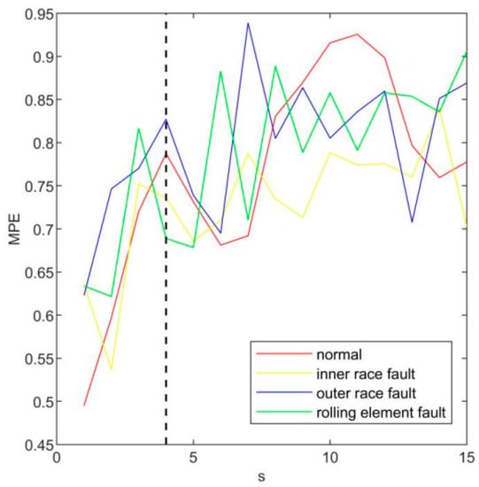
Figure 9.
The MPE of imf3.
Using the feature vector construction method proposed in this paper, the corresponding optimal multi-scale permutation entropy of all samples is calculated to form the feature vector. There are 50 × 4 × 3 permutation entropy, 50 × 4 feature vectors. 30 × 4 feature vectors of the training samples are used to train the model of the support vector machine and optimize its parameters. 20 × 4 feature vectors of the test samples are used as unknowns for the final classification test. Four sets of feature vectors are given here, as shown in Table 8. The digital labels 1~4 in the table represent the normal state, inner ring fault, outer ring fault, and rolling element fault, respectively.
Table 8.
The feature vectors and labels.
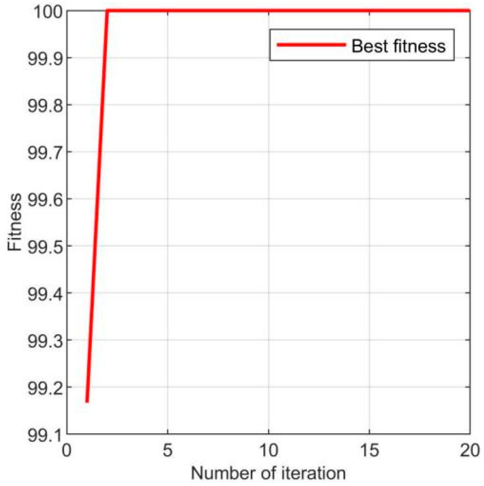
One hundred and twenty feature vectors of training sets similar to Table 8 are input into SOA-SVM for training. As can be seen from Figure 10, after two iterations, the fitness value can reach 100%. The optimum parameters C and g are 35.609 and 1.991, respectively.

Figure 10.
The convergence curve of the SOA-SVM method.
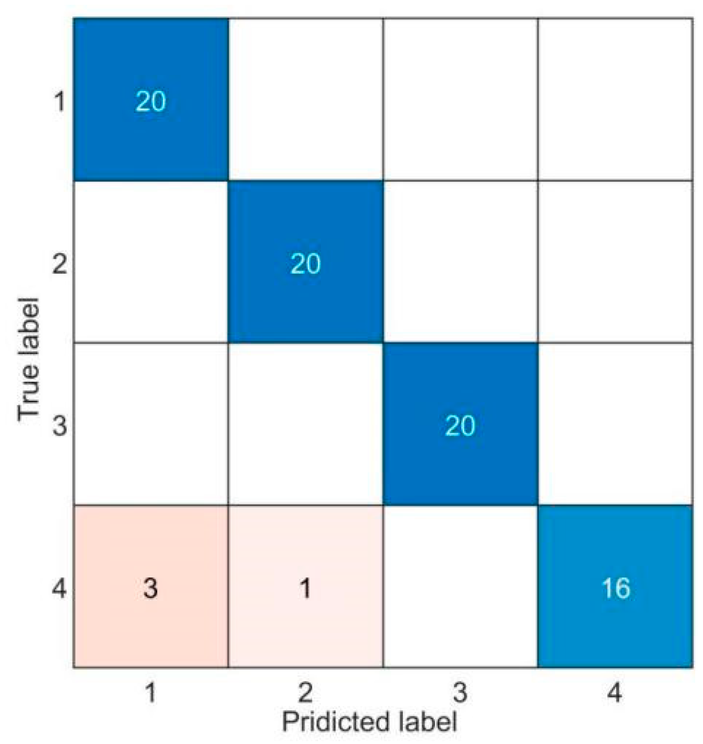
The learned detection entity model is used to identify rolling bearing faults. Figure 11 shows the confusion matrix results obtained by applying the WOA-VMD-SOA-SVM approach in four different common scenarios. There is an incorrectly classified sample, which identifies the rolling element fault as the inner ring fault, and the detection set ‘s ultimate identification accuracy is 98.75%. The findings show that the fault-detection approach can correctly identify common rolling bearing defects in a variety of conditions.
Figure 11.
The confusion matrix of the WOA-VMD-SOA-SVM method.
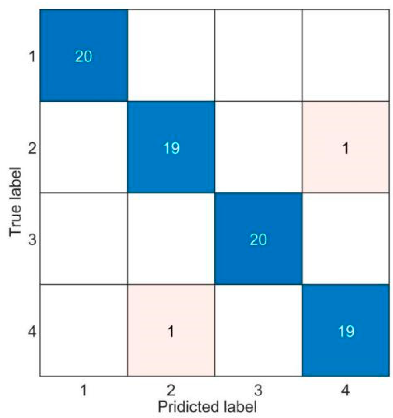
To better verify the effectiveness of the improved VMD optimization algorithm, WOA-VMD and non-boosted VMD are compared in this paper. The VMD primary parameter K is set to 8, and α is set to 2000 in this case. Figure 12 shows the results of the confusion matrix applying the VMD-SOA-SVM fault-detection way. The accuracy on the detection set is 95.00%. Figure 13 shows the results of the confusion matrix applying the WOA-VMD-PSO-SVM fault-detection approach. The accuracy on the detection set is 97.50%. According to the comparison of Figure 10 and Figure 11, it can be shown that the WOA-VMD method’s actual effect is stronger than that of the non-improved VMD method, indicating that the WOA-VMD method can more precisely collect the information content of the common rolling bearing’s fault characteristics. In addition, according to the comparison of Figure 10 and Figure 12, it can be shown that the actual effect of using WOA-VMD-SOA-SVM is better than that of applying WOA-VMD-PSO-SVM, indicating that SOA is more powerful than PSO.

Figure 12.
The confusion matrix of the VMD-SOA-SVM method.

Figure 13.
The confusion matrix of the WOA-VMD-PSO-SVM method.
4. Conclusions
In this article, we mentioned a fault-detection method for rolling bearings that integrated WOA-VMD, multi-scale permutation entropy, and the SOA-SVM algorithm. Rolling bearing fault detection and analysis were carried out from the fields of data processing, fault feature extraction, and fault feature recognition.
The key parameters of VMD were obtained using the whale optimization algorithm, and then the information of fault characteristics was obtained using the improved VMD method. According to the results, WOA-VMD may reasonably retrieve the fault information content of rolling bearings. In feature extraction, we found that the scale factors s were 7, 9, and 4, respectively, in order to obtain the optimal multi-scale permutation entropy of three imfs. The SOA approach was used to optimize the parameters of the penalty factor C and the kernel function g in the SVM fault-detection entity model. The results showed that the SOA-SVM method had good classification characteristics, and the mean diagnosis accuracy can reach 98.75%. Compared with the results of other methods, it can be seen that this method can reasonably diagnose different damage types of the rolling bearings. This method can accurately distinguish different faults of rolling bearings. However, for different fault degrees of the same fault type, its classification accuracy needs to be improved.
In the future work, we will focus on building a test service platform for mining fans, collecting mechanical vibration data signals of rolling bearings and certifying the feasibility analysis of applying the methods mentioned in the article to fault detection of mining fans.
Author Contributions
Conceptualization, X.Z. and H.W.; methodology, H.W.; software, H.W. and M.R.; validation, M.H. and L.J.; formal analysis, M.H.; investigation, L.J.; resources, M.H.; data curation, M.R.; writing—original draft preparation, H.W.; writing—review and editing, X.Z.; visualization, H.W.; supervision, M.R.; project administration, M.H.; and funding acquisition, X.Z. All authors have read and agreed to the published version of the manuscript.
Funding
This research was supported by funds by the National Natural Science Foundation of China No. 51774293.
Data Availability Statement
This research used the published rolling bearing datasets of Western Reserve University. The access of the datasets is https://engineering.case.edu/bearingdatacenter/welcome (accessed on 7 May 2022).
Acknowledgments
The authors appreciate the editor’s helpful remarks and ideas, as well as those of the anonymous reviewers. The authors also would like to thank the National Natural Science Foundation of China No. 51774293 for its support.
Conflicts of Interest
The authors declare no conflict of interest.
Abbreviations
| K | decomposition levels |
| α | secondary penalty factor |
| whale location vector | |
| r | random number |
| lower boundary | |
| ub | upper boundary |
| p | random number |
| , | coefficient vectors |
| best solution obtained so far | |
| element-by-element multiplication | |
| probability distribution | |
| envelope entropy | |
| s | scale factor |
| N | time-series length |
| m | encapsulation dimension |
| time delay | |
| n | number of samples |
| xi | the ith input value |
| the normal vector of the hyperplane | |
| m | offset |
| Λ | high-dimensional space |
| Ψ | nonlinear mapping |
| ξi | relaxation variable |
| k(xi,xj) | kernel function |
| C | penalty factor |
| g | kernel width |
| position of seagulls | |
| number of iteration | |
| initial position of the seagull | |
| the direction of the best position | |
| new position where the seagull meets three conditions | |
| u,v | correlation constant |
| θ | angle |
| the best seagull position |
References
- He, C.; Wu, T.; Gu, R.; Jin, Z.; Ma, R.; Qu, H. Rolling bearing fault diagnosis based on composite multiscale permutation entropy and reverse cognitive fruit fly optimization algorithm—Extreme learning machine. Measurement 2020, 173, 108636. [Google Scholar] [CrossRef]
- Zmarzły, P. Multi-Dimensional Mathematical Wear Models of Vibration Generated by Rolling Ball Bearings Made of AISI 52100 Bearing Steel. Materials 2020, 13, 5440. [Google Scholar] [CrossRef] [PubMed]
- Liu, H.; Han, M. A fault diagnosis method based on local mean decomposition and multi-scale entropy for roller bearings. Mech. Mach. Theory 2014, 75, 67–78. [Google Scholar] [CrossRef]
- Zheng, J.; Cheng, J.; Yang, Y.; Luo, S. A rolling bearing fault diagnosis method based on multi-scale fuzzy entropy and variable predictive model-based class discrimination. Mech. Mach. Theory 2014, 78, 187–200. [Google Scholar] [CrossRef]
- Feng, Z.; Zuo, M.J. Vibration signal models for fault diagnosis of planetary gearboxes. J. Sound Vib. 2012, 331, 4919–4939. [Google Scholar] [CrossRef]
- Huang, N.E.; Shen, Z.; Long, S.R.; Wu, M.C.; Shih, H.H.; Zheng, Q.; Yen, N.-C.; Tung, C.C.; Liu, H.H. The empirical mode decomposition and the Hilbert spectrum for nonlinear and non-stationary time series analysis. Proc. Math. Phys. Eng. Sci. 1998, 454, 903–995. [Google Scholar] [CrossRef]
- Du, Q.; Yang, S. Improvement of the EMD method and applications in defect diagnosis of ball bearings. Meas. Sci. Technol. 2006, 17, 2355–2361. [Google Scholar] [CrossRef]
- Wang, H.; Chen, J.; Dong, G. Feature extraction of rolling bearing’s early weak fault based on EEMD and tunable Q-factor wavelet transform. Mech. Syst. Signal Process. 2014, 48, 103–119. [Google Scholar] [CrossRef]
- Dragomiretskiy, K.; Zosso, D. Variational Mode Decomposition. In IEEE Transactions on Signal Processing; A Publication of the IEEE Signal Processing Society; IEEE: Piscataway, NJ, USA, 2014. [Google Scholar]
- Zhang, Z.; Zhang, X.; Zhang, P.; Wu, F.; Li, X. Compound fault extraction method via self-adaptively determining the number of decomposition layers of the variational mode decomposition. Rev. Sci. Instrum. 2018, 89, 085110. [Google Scholar] [CrossRef]
- Guo, Z.; Liu, M.; Wang, Y.; Qin, H. A New Fault Diagnosis Classifier for Rolling Bearing United Multi-Scale Permutation Entropy Optimize VMD and Cuckoo Search SVM. IEEE Access 2020, 8, 153610–153629. [Google Scholar] [CrossRef]
- Gu, R.; Chen, J.; Hong, R.; Wang, H.; Wu, W. Incipient fault diagnosis of rolling bearings based on adaptive variational mode decomposition and Teager energy operator. Measurement 2020, 149, 106941. [Google Scholar] [CrossRef]
- Li, J.; Chen, W.; Han, K.; Wang, Q. Fault Diagnosis of Rolling Bearing Based on GA-VMD and Improved WOA-LSSVM. IEEE Access 2020, 8, 166753–166767. [Google Scholar] [CrossRef]
- Richman, J.S.; Moorman, J.R. Physiological time-series analysis using approximate entropy and sample entropy. Am. J. Physiol. 2000, 278, H2039–H2049. [Google Scholar] [CrossRef] [PubMed] [Green Version]
- Bandt, C.; Pompe, B. Permutation Entropy: A Natural Complexity Measure for Time Series. Phys. Rev. Lett. 2002, 88, 174102. [Google Scholar] [CrossRef] [PubMed]
- Costa, M.; Goldberger, A.L.; Peng, C.-K. Multiscale Entropy Analysis of Complex Physiologic Time Series. Phys. Rev. Lett. 2002, 89, 068102. [Google Scholar] [CrossRef] [PubMed] [Green Version]
- Aziz, W.; Arif, M. Multiscale Permutation Entropy of Physiological Time Series. In Proceedings of the 2005 Pakistan Section Multitopic Conference, Karachi, Pakistan, 24–25 December 2005. [Google Scholar]
- Zheng, J.; Cheng, J.; Yang, Y. Multiscale Permutation Entropy Based Rolling Bearing Fault Diagnosis. Shock Vib. 2014, 2014, 154291. [Google Scholar] [CrossRef]
- Shuang, L.; Meng, L. Bearing Fault Diagnosis Based on PCA and SVM. In Proceedings of the 2007 International Conference on Mechatronics and Automation, Harbin, China, 5–8 August 2007. [Google Scholar]
- Hou, Z.R. Rolling Bearing Fault Diagnosis Based on Wavelet Packet and Improved BP Neural Network for Wind Turbines. Appl. Mech. Mater. 2013, 347–350, 117–120. [Google Scholar] [CrossRef]
- Qin, B.; Sun, G.D.; Zhang, L.Y.; Wang, J.G.; Hu, J. Fault Features Extraction and Identification based Rolling Bearing Fault Diagnosis. J. Phys. Conf. Ser. 2017, 842, 012055. [Google Scholar] [CrossRef] [Green Version]
- Wang, Z.; Yao, L.; Cai, Y. Rolling bearing fault diagnosis using generalized refined composite multiscale sample entropy and optimized support vector machine. Measurement 2020, 156, 107574. [Google Scholar] [CrossRef]
- Wang, R.; Zhang, Z.; Xia, Z.; Miao, J.; Guo, Y. A new approach for rolling bearing fault diagnosis based on EEMD hierarchical entropy and improved CS-SVM. In Proceedings of the 2019 Prognostics and System Health Management Conference (PHM-Qingdao), Qingdao, China, 25–27 October 2019. [Google Scholar]
- Liu, H.; Xiang, J. A Strategy Using Variational Mode Decomposition, L-Kurtosis and Minimum Entropy Deconvolution to Detect Mechanical Faults. IEEE Access 2019, 7, 70564–70573. [Google Scholar] [CrossRef]
- Ma, H.; Tong, Q.; Zhang, Y. Applications of Optimization Parameters VMD to Fault Diagnosis of Rolling Bearings. Zhongguo Jixie Gongcheng/China Mech. Eng. 2018, 29, 390–397. [Google Scholar]
- Mirjalili, S.; Lewis, A. The Whale Optimization Algorithm. Adv. Eng. Softw. 2016, 95, 51–67. [Google Scholar] [CrossRef]
- Yang, W.; Yang, Z.; Chen, Y.; Peng, Z. Modified Whale Optimization Algorithm for Multi-Type Combine Harvesters Scheduling. Machines 2022, 10, 64. [Google Scholar] [CrossRef]
- Tang, G.J.; Wang, X.L. Parameter optimized variational mode decomposition method with application to incipient fault diagnosis of rolling bearing. J. Xi’an Jiaotong Univ. 2015, 49, 73–81. [Google Scholar]
- Ma, P.; Zhang, H.; Fan, W.; Wang, C. Fault diagnosis using an improved fusion feature based on manifold learning for wind turbine transmission system. J. Vibroeng. 2019, 21, 1859–1874. [Google Scholar] [CrossRef]
- Liang, T.; Lu, H.; Sun, H. Application of Parameter Optimized Variational Mode Decomposition Method in Fault Feature Extraction of Rolling Bearing. Entropy 2021, 23, 520. [Google Scholar] [CrossRef] [PubMed]
- Li, Y.; Xu, M.; Wei, Y.; Huang, W. A new rolling bearing fault diagnosis method based on multiscale permutation entropy and improved support vector machine based binary tree. Measurement 2016, 77, 80–94. [Google Scholar] [CrossRef]
- Matilla-García, M. A non-parametric test for independence based on symbolic dynamics. J. Econ. Dyn. Control 2007, 31, 3889–3903. [Google Scholar] [CrossRef]
- Dhiman, G.; Kumar, V. Seagull optimization algorithm: Theory and its applications for large-scale industrial engineering problems. Knowl. Based Syst. 2018, 165, 169–196. [Google Scholar] [CrossRef]
- Wang, J.; Li, Y.; Hu, G. Hybrid seagull optimization algorithm and its engineering application integrating Yin–Yang Pair idea. Eng. Comput. 2021, 38, 2821–2857. [Google Scholar] [CrossRef]
- Jiyong, T.A.N.; Xuefeng, C.H.E.N.; Zhengjia, H.E. Impact Signal Detection Method with Adaptive Stochastic Resonance. J. Mech. Eng. 2010, 46, 61–67. [Google Scholar]
- Li, J.; Chen, X.; He, Z. Adaptive stochastic resonance method for impact signal detection based on sliding window. Mech. Syst. Signal Process. 2013, 36, 240–255. [Google Scholar] [CrossRef]


Publisher’s Note: MDPI stays neutral with regard to jurisdictional claims in published maps and institutional affiliations. |
© 2022 by the authors. Licensee MDPI, Basel, Switzerland. This article is an open access article distributed under the terms and conditions of the Creative Commons Attribution (CC BY) license (https://creativecommons.org/licenses/by/4.0/).