Article

Dynamic Scaling of a Wing Structure Model Using Topology Optimization

by
Éder Oliveira
1,
Abdolrasoul Sohouli
2,
Frederico Afonso
1,
Roberto Gil Annes da Silva
3 and
Afzal Suleman
1,2,*
1
IDMEC, Instituto Superior Técnico, Universidade de Lisboa, Av. Rovisco Pais, No. 1, 1049-001 Lisboa, Portugal
2
Department of Mechanical Engineering, University of Victoria, Stn. CSC, Victoria, BC V8W 2Y2, Canada
3
Department of Aeronautical Engineering, Aeronautics Institute of Technology, Praça Marechal Eduardo Gomes, 50, Vila das Acacias, Sao Jose dos Campos 12228-900, SP, Brazil
*
Author to whom correspondence should be addressed.
Machines 2022, 10(5), 374; https://doi.org/10.3390/machines10050374
Submission received: 10 April 2022 / Revised: 8 May 2022 / Accepted: 12 May 2022 / Published: 16 May 2022
(This article belongs to the Special Issue Dynamic Stability Analysis of Aerospace Structures)

Abstract

:
In this paper, a dynamic scaling methodology is introduced to devise reduced scaled models of aircraft with the objectives of minimizing the development cost and exploring the design space. A promising way to accomplish this is using Topology Optimization (TO) for Additive Manufacturing (AM). Here, TO is employed to design a reduce scale model by matching its natural frequencies and mode shapes to those of a full scale model. Different TO strategies based on density approach are tested with the goal of achieving a dynamically scaled structure that can be manufactured. To achieve this goal, the TO solution should be free from intermediate densities, which is observed for some TO strategies but not all. When no penalization factor is applied: (i) the relative difference between natural frequencies is less than 1% and (ii) the estimated Modal Assurance Criteria (MAC) metric to evaluate the correlation between mode shapes is close to the ideal identity matrix. These results demonstrate the effectiveness of the dynamic scaling methodology. However, when using a penalization factor to avoid intermediate densities, the dynamic behavior correlation between full and scaled models degrades. This trend is more visible in the MAC metric, where off-diagonal terms above 20% and diagonal terms below 90% appear.

1. Introduction

Designing any complex new product requires several working hours, including expensive experimental tests, that usually implies a high Research and Development (R&D) cost. A good example is an aircraft design project, where the development cost represents a significant part of the final product cost, which will depend on selling several units to dilute its price on each sale. Furthermore, the aviation industry is studying more environmentally sustainable aircraft to reduce its carbon footprint. Some of the proposed solutions are unconventional such as the Blended Wing Body (BWB) [1] or the Truss-Braced Wing (TBW) [2]. These designs are likely to have a different dynamic behavior than the conventional tube and wing configuration. Therefore, it is important to study and develop them in an integrated way using not only Multidisciplinary Design Optimization (MDO) strategies [3], but also experimental test beds such as wind tunnel [4] or flight test [5] models. In this paper, the focus is on devising scaled test models that are able to mick the dynamic behavior of its full size counterpart. Producing meaningful scaled models to test unconventional features at early design stages might lead to the early detection of problems and avoid expensive redesigns after performing tests with a full-size model.
A dynamic scaling methodology is proposed to design meaningful reduced scale models to be experimentally tested. This methodology aims at designing a scaled model by means of Topology Optimization (TO) for Additive Manufacturing (AM) that presents the same dynamic behavior of the full size model. To obtain dynamic similitude [6] the mode shapes and associated natural frequencies should be adequately scaled down and matched. Dynamic scaling methodologies have been applied to devise both wind tunnel [7,8] and flight [9,10,11,12] test models for evaluating aeroelastic behavior of unconventional designs. As seen in previous publications [13,14], an adequate dynamic scaling strategy when combined with a suitable selection of aerodynamic parameters enables aeroelastic similarity for some flow conditions, even though Mach and Reynolds number similarities are difficult to ensure [15,16]. Thus, achieving dynamic similitude is a key step towards aeroelastic similitude. Most of these methodologies [9,11,13,14] recur to optimization routines for replicating the dynamic behavior of the full size model in the scaled one by means of sizing a prescribed structural layout [17] with an exact scaled down external geometry. Alternative strategies such as changing the wing planform [12] by means of MDO or using TO [18] has been recently proposed.
TO is seen as a promising numerical method to be included in a dynamic scaling methodology given the higher design freedom and the possible synergies with AM. Topologically optimizing a structure [19] has proved to be an efficient tool in minimizing weight for several engineering fields, including aeronautics [20]. Associated to the advantage of a higher design freedom is the problem dimension, which is also higher and often leads to complex designs to manufacture. However, its interest has exponentially grown in the past years with the recent progress in AM [21], including aeronautical applications such as Unmanned Aerial Systems (UAS) [22,23]. Even though substantial progress have been made to allow for manufacturing complex topologically optimized parts; issues such as overhanging structures, poor surface quality, porous infill layouts and intermediate densities [21,24,25,26,27] should be addressed when designing a part. These issues if handled in a post-processing phase for a dynamic scaling problem, are likely to modify both mode shapes and associated frequencies.
In this work, the main objective is to propose a dynamic scaling methodology that recurs to TO, instead of the commonly used sizing optimization, to design scaled models that represent the dynamic behavior of a full size model. To the authors best knowledge there are very few papers in the literature employing TO in the process of dynamically scaling structures which might lead to synergies with additive manufacturing. The effect of a penalization factor to avoid intermediate densities on the ability to replicate this dynamic behavior is also assessed.
The remaining of this paper is organized as follows. In Section 2, the proposed dynamic scaling methodology is introduced. Then its application to several test cases is discussed in Section 3 and the concluding remarks are presented in Section 4.

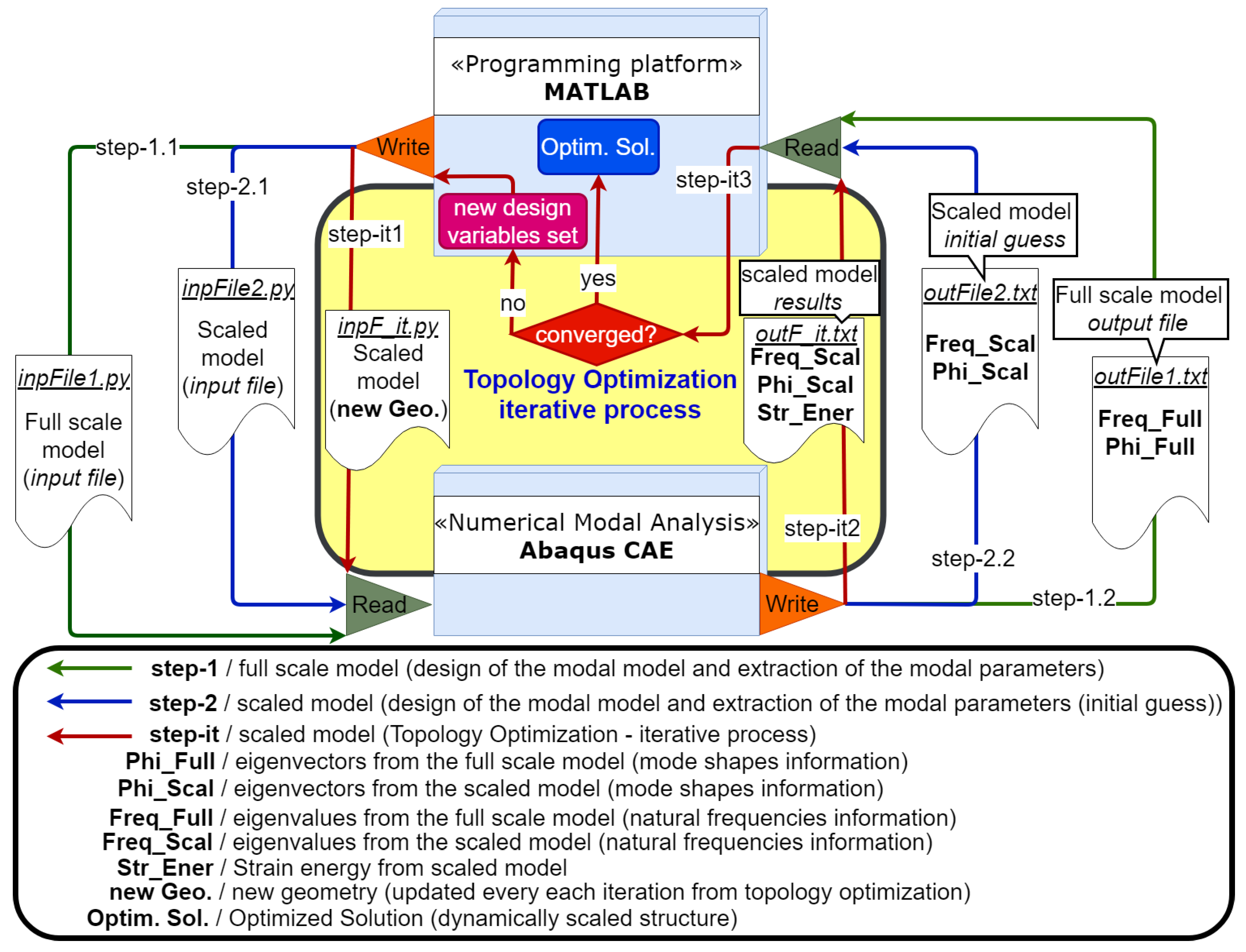
2. Dynamic Scaling Methodology

A dynamic scaling methodology comprising 3 main steps is proposed. First the full scaled model is defined and its modal parameters are determined (step-1). Based on this model and a predefined set of scaling factors, the scaled model is first built (step-2) and its structure is then topologically optimized to ensure that dynamic similarity between models (step-it). The flowchart of this methodology is depicted in Figure 1, where the reader should follow a counter-clockwise direction from the external green lines (step-1) passing through the blue lines (step-2) and converging to the red lines in the yellow box, representing the iterative topology optimization process (step-it). A detailed explanation of the proposed methodology applied to a wing model is given in the subsequent sub-sections.

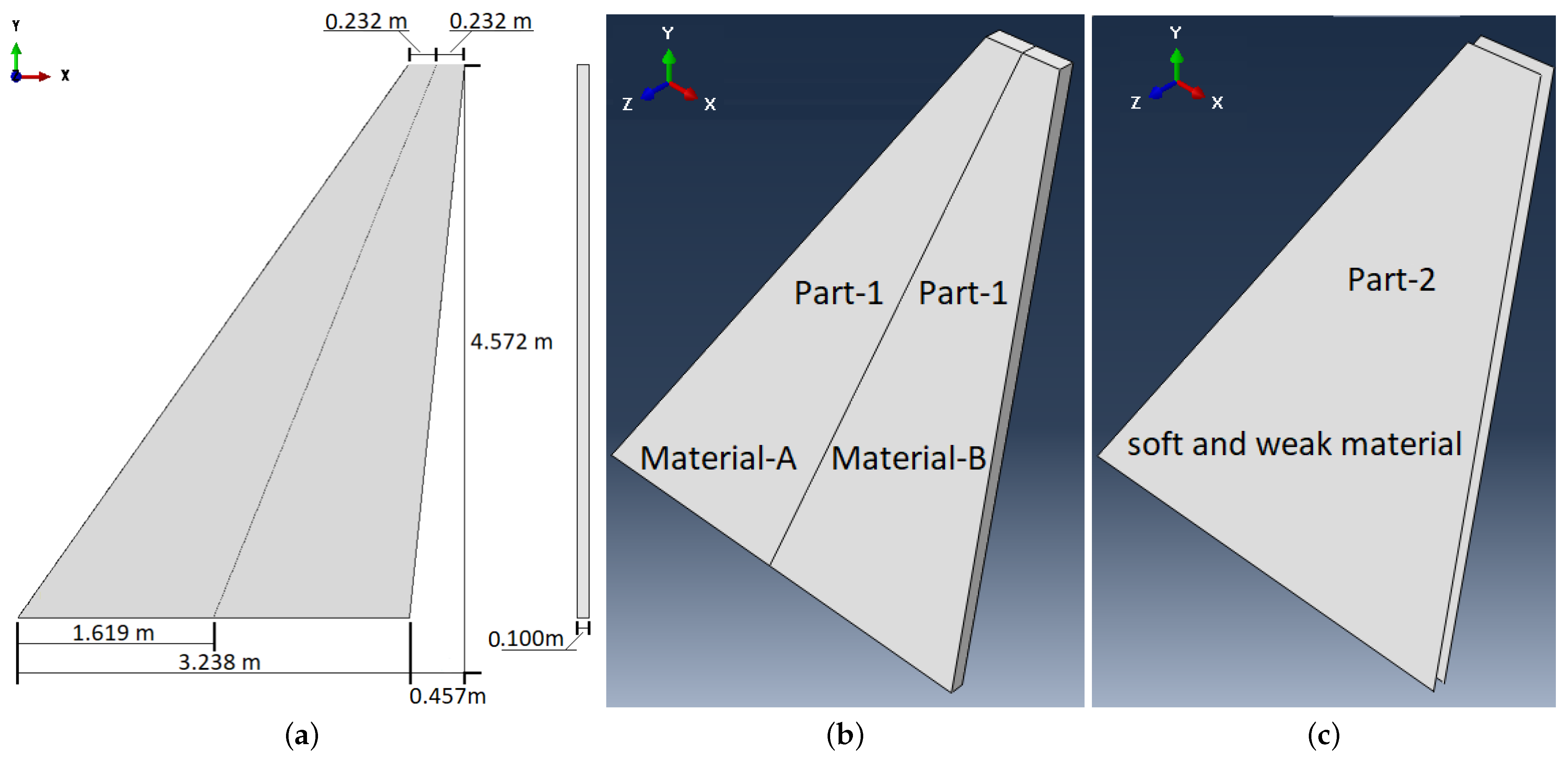
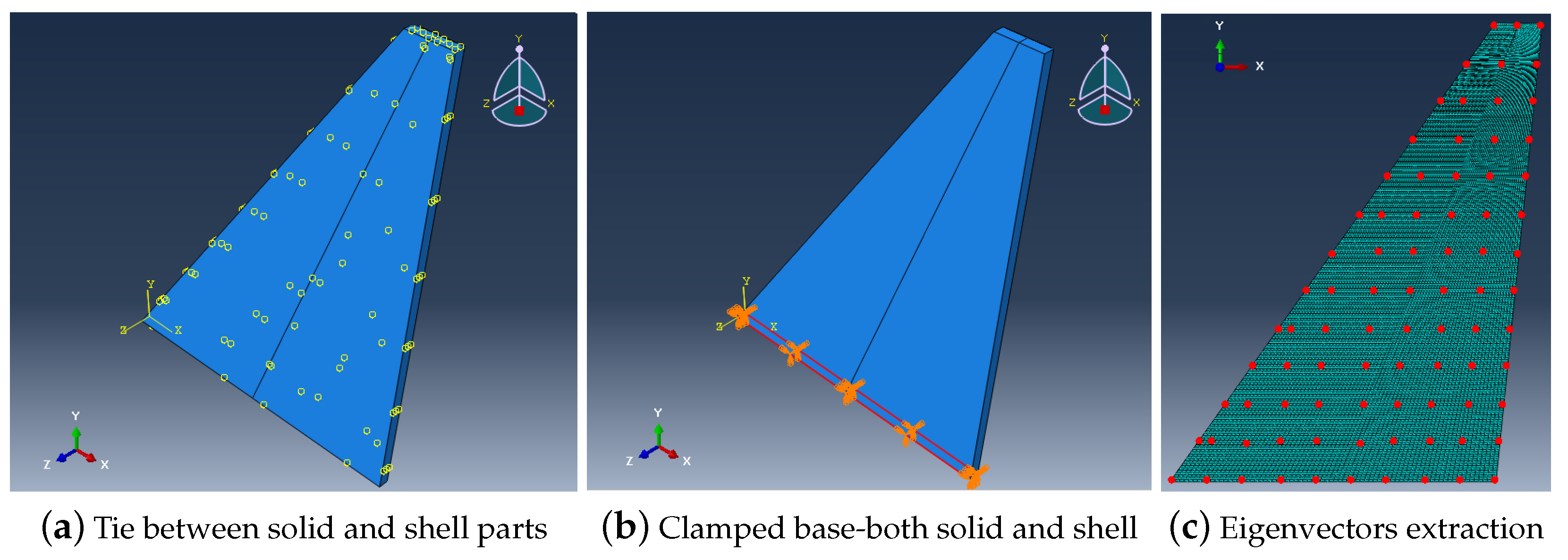
2.1. Full Scale Model

For the full scale model the wing geometry proposed by [28] is scaled up to the dimensions depicted in Figure 2. Regarding the structure two parts are defined: an internal solid part (Part-1 in Figure 2b); and an external part modeled as a shell (Part-2 in Figure 2c). The external shell represents the wing skin and will be kept unaltered when scaled down to maintain the aerodynamic shape for a future aeroelastic scaling. The material properties of the skin are set to be “weaker” than those of the internal solid part. Two “fictitious” sub-parts with different material properties (Material-A and Material-B), as depicted in Figure 2b, are defined for the internal structure (this is a purely academic problem since no boundary condition between the different materials is applied.) This is conducted to enable the easy adjust of the contrast between different sub-parts to control the problem’s difficulty in reaching dynamic similarity. For instance, if two considerably different metals (e.g., Al and Ti) are chosen for the two sub-parts, it will be more difficult to reach the desired dynamic similarity than if the same material is used for both sub-parts.
A Finite Element Method (FEM) model of the above described wing is built in Abaqus®. The skin and solid parts are modeled using Shell S4R and Solid C3D8R, respectively. Regarding the boundary conditions, these two parts are tied between each other, as illustrated in Figure 3a, and all degrees of freedom (DoFs) at the wing root are clamped, as depicted in he Figure 3b. To compute the natural frequencies (eigenvalues) and corresponding mode shapes (eigenvectors) necessary for the dynamic scaling methodology a modal analysis problem is solved. The mode shapes are extracted from several points distributed on the wing (marked in Figure 3c), such that those points are able to reproduce any mode shape in the range of interest. Here, only the first five mode shapes are considered for the cases analyzed.
A mesh size of 58.9k elements was defined for the FEM model as a compromise between computational cost and accuracy for the modal analysis problem, after performing a mesh convergence study. With this mesh the simulation takes around 4 minutes (Workstation with 24 cores Intel(R) Xeon(R) E5-2620 v2 @2.10 GHz totaling @50.4 GHz with 32 GB of RAM (Random Access Memory).) and the errors relative to the finest mesh considered are lower than 2%, as one can see from Figure 4.
After a mesh is chosen, this process is carried out automatically in the dynamic scaling methodology (Figure 1) be means of a python script (inpFile1.py) that is built in Matlab® and runs Abaqus®. The resulting modal information is written in a file (outFile1.txt) that will be read to establish the target parameters for the scaled model.

2.2. Scaled Model

There are several strategies that can be applied to derive the required set of scaling factors ( λ ) to define a dynamically scaled model. To form this set, the fundamental quantities of mass, length and time should be included in the three primary quantities chosen to derive the scaled model. One possibility is to define length (l), density ( ρ ) and pressure (p) in the scaled model as follows:
λ l = l s l f λ ρ = ρ s ρ f λ p = p s p f ,
where the subscripts s and f denote scaled and full size models, respectively. The natural frequency scaling factor can be derived from the above factors, resulting in:
λ ω = λ p λ ρ λ l 2 .
Here, for simplicity the density and pressure scaling factors are unitary and the scaled model is 10 times smaller than the full scale in size (i.e., λ l = 0.1 ). With these assumptions, the scaled model frequencies are targeted to be 10 times higher than those of the full scale (i.e., λ ω = 10 ). To ensure an exact dynamic similarity also the damping factors and mode shapes should be matched. Since structural damping is difficult to model numerically it is often neglected. The mode shapes of full size and scaled models can be matched using the Modal Assurance Criteria (MAC) if a gradient free optimizer (e.g., a genetic algorithm) is used, which will be time consuming given the number of design variables involved in a topology optimization problem. For these reasons, neither damping nor mode shapes are directly matched in the dynamic scaling methodology here proposed. Nevertheless, the MAC is used to track the correct mode shapes for matching the natural frequencies, in the proposed methodology. MAC is a statistical indicator that is widely used to provide a quantitative comparison between two mode shapes [29] and can be expressed as follows:
MAC ( A , B ) = Ψ A T × Ψ B 2 Ψ A T × Ψ A × Ψ B T × Ψ B ,
where Ψ A and Ψ B denote the eigenvector A and B, respectively. A n × n square matrix can be constructed by comparing two sets of n eigenvectors, which ideally should be an identity matrix to ensure a perfect correlation between the two sets of mode shapes, for instance of the full-size and scaled models.
Based on the previous considerations, a scaled model 10 times smaller in size than the full scale one is built in Abaqus®. Despite the geometry is merely a scaled down of the previous model, now only one material is used and the internal geometry needs to be prepared for optimization. To this end, a proper grid is needed to define the design variables using datum planes. For practical reasons, the internal mesh is much coarser than the one used for the full scale model since each of the internal mesh elements will be set as a design variable. Two different grids, depicted in Figure 5, are considered, (18, 24, 1) and (54, 72, 1), where (X, Y, Z) indicate the number of grid cells in x, y and z planes, respectively. It is worth to note that only the grid cells belonging to the wing geometry are set as design variables. When designing this grid, attention should be taken in regard to: (i) the points chosen to extract the mode shape information for comparison with the full scale model; and (ii) the mesh quality in the most incline boundary.
Again, python scripts, inpFile2.py and inpF_it.py, are created to generate and run the FEM model automatically to initialize the scaling process and during the optimization, respectively. In what concerns the output files: outFile2.txt provides the same modal information as before; while outF_it.txt besides storing the mode shapes and natural frequencies also stores information regarding strain energy for the topology optimization.

2.3. Topology Optimization

Topology optimization is used to determine an internal topological layout for the scaled model that minimizes the relative differences between the first five natural frequencies of full and scaled models. The mathematical statement of this optimization problem is the following:
minimize f x = i = 1 m 1 ω s i 2 x ω t i 2 2 w . r . t 0 x 1 ,
where x is the vector of design variables, ω denotes natural frequency, subscripts s and t refer to scaled and target models, respectively, and m represents the number of mode shapes considered, which in this case is five. The vector of design variables ( x ) represents the description of material, which follows the RAMP (Rational Approximation of Material Properties) [30] method for both the elasticity modulus (E) and the Poisson ratio ( ν ) and the SIMP (Simplified Isotropic Material with Penalization) method [31] for the density ( ρ ), as follows:
E x j = E 0 + x j 1 + p 1 x j E m E 0 ;
ν x j = ν 0 + x j 1 + p 1 x j ν m ν 0 ;
ρ x j = ρ 0 + x j p ρ m ρ 0 .
In the above equations: j denotes an arbitrary patch or element j; p is the penalization factor; the subscript m represents the material chosen for the scaled model; E 0 , ν 0 and ρ 0 are properties corresponding to a material with low stiffness and mass. Each x j can assume a value within 0 (void) and 1 (solid), although to avoid singularities a minimum value of 0.0001 is established. In all the optimizations performed, the initial value for each x j is set to 0.5. The penalization factor is defined by default as 1.
Since the mode shape sequence can change during the topology optimization process [32], a mode tracking procedure based on the MAC should be employed. To this end, the first eight eigenvectors (instead of using only five) are used to compute the MAC metric and sort the modes such that on the diagonal terms have the highest correlation possible.
The Interior Point OPTimizer (IPOPT) algorithm is used to solve this topology optimization problem. IPOPT is a gradient-based algorithm developed by [33] that is able to deal with large nonlinear optimization problems, such as the one of this work. Since IPOPT is a gradient-based optimizer it requires computing the sensitivities with respect to the design variables. The natural frequencies are computed by solving the eigenvalue problem:
K ω i 2 M Ψ i = 0 with i = 1 , , m .
In the above equation both the stiffness matrix K and mass matrix M depend on the design variables x , thus also the eigenvalues ω and eigenvectors Ψ depend on the design variables. By differentiating the eigenvalue problem with respect to the design variables, the following is obtained:
K ( x ) x ω i 2 M ( x ) x + ω i 2 ( x ) x M Ψ i + K ω i 2 M Ψ i x = 0 .
After some algebraic manipulation the following expression emerges:
ω i 2 ( x ) x = Ψ i T K ( x ) x ω i 2 M ( x ) x Ψ i .

3. Results

In order to evaluate the proposed methodology adequacy for performing dynamic scaling using a single material topology optimization strategy, eight test cases are conducted. These test cases are also important to identify the proposed dynamic scaling methodology limitations. The first two cases, presented in Section 3.1, consists of simply introducing a difference between the material properties of both models (full and scaled), which increases from the first to the second case. Then, to assess the impact of design space size the two different grids mentioned before are compared in Section 3.2. Finally, the strategy of increasing the penalization factor to avoid intermediate densities is discussed in Section 3.3 using 4 different values.

3.1. Material Influence Test Case

Before defining this test case, it is worth to recall that the full scale model is composed of two parts, an external shell (Part-2) and an internal solid part (Part-1) made of two materials (A and B), as illustrated in Figure 2; while the scaled model consists of an internal part made of a single material and an external shell. Furthermore, the scaled model shell remains unmodified during the optimization process.
As mentioned earlier the goal of this sub-section is to evaluate the influence of varying the difference between the material properties of both models. Two case studies, with increasing difficulty, are conducted for this purpose, using the most coarse design grid (18, 24, 1). In the first case study (Case 1), the proposed dynamic scaling methodology is tested considering small differences between the material properties of the full scale model and the scaled one, as presented in Table 1. These difference are then increased for the second case (Case 2) as can be observed also from Table 1. In what concerns solid A the same differences between material properties as for Case 1 are maintained, however for solid B these differences are increased and consequently making it more difficult to achieve dynamic similarity. Since unitary scaling factors are defined for both density and pressure the material properties of the target and full size models are the same.
For Case 1, the highest differences in terms of elasticity modulus is observed for the shell part ( 39 % ); while for the density and Poisson ratio, the solid part made of material A presents the highest differences ( 19 % and 17 % , respectively). It is important to mention that although the shell thickness is 1 mm in the full size model, its reduced size counterpart is four times higher (i.e., 4 mm) to further difficult the dynamic scaling process. This last consideration is also applied in Case 2. Even though a difference of 60,506% in the elasticity modulus is considered for the shell in Case 2, its influence on the results is reduced when compared with the internal solids A and B given its small thickness value.
The optimization for Case 1 reached a reasonable good solution just after performing 16 iterations, as one can see from the convergence history in Figure 6. After these 16 iterations, despite the solution fluctuates slightly the best result is reached at the 26th iteration with an objective function value of 2.80 × 10 4 . As expected, Case 2 presents a slightly slower convergence than Case 1 given the higher differences in material properties between not only target and scaled models but also between solids A and B. The lowest objective function value ( 3.78 × 10 4 ) is reached at 49th iteration. For both cases, the maximum number of iterations is set to 60.
These low objective function values indicate that a very small difference between natural frequencies is reached, which is demonstrated in Table 2. In fact, the relative error between the target and obtained frequencies is lower than 0.1% for both case studies.
To verify if the mode shapes from both models also match, one can use the previously mentioned MAC metric. Despite not directly expressed in the objective function, the MAC is used to track the right mode shapes to compare the associated natural frequencies. This metric is illustrated for the best result of Case 1 in Figure 7a, where the less correlated mode shape (5th mode shape) presents 94 % of correlation concerning its peer (diagonal values), and higher correlation between each other (off-diagonal values) was 10.6 % . A similar correlation is found for Case 2 as depicted in Figure 7b.
The results obtained indeed indicate that the matching of both the natural frequencies and mode shapes is successfully accomplished even for the most coarse design grid (18, 24, 1). This proves that the developed methodology can be used for dynamic scaling with similar assumptions to those considered in this case study. For this case study, the material properties of the solid parts in the scaled model differ only slightly from the target material properties, which are equal to ones of the full scale model since unitary density and pressure scaling factors are defined. The correlation between mode shapes degrades slightly with the increase of these differences in material properties of the solid parts.
Regarding the topologically optimized internal structures, the solutions for both cases are very similar as illustrated in Figure 8.

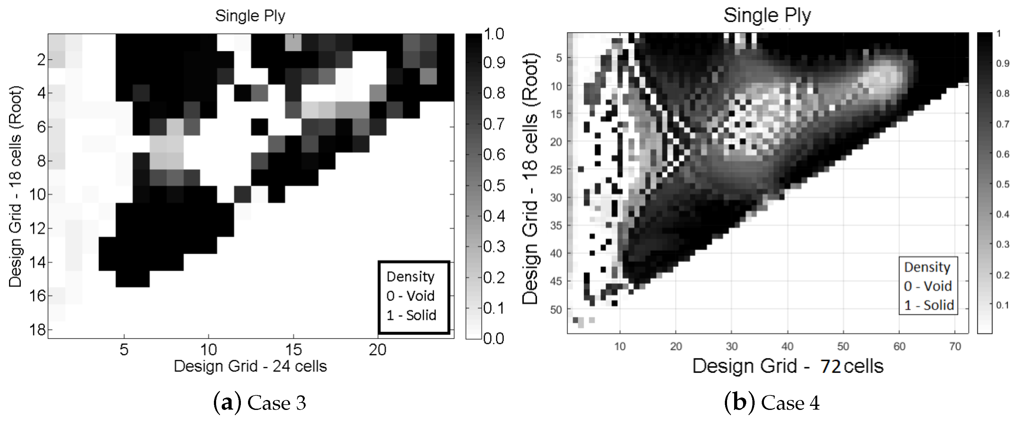
3.2. Design Space Test Case

The objective now is to evaluate the impact of increasing the number of design variables on dynamic similarity for a more challenging test case. For this purpose the two design grids presented in Section 2.2 are used. In the previous case studies, the material properties were fictitious and adapted to analyze differences between models. On the other hand, in the current test case existing materials are set for both full and scaled models, which increases the differences in material properties. To increase the difficult of reaching dynamic similarity, the full scale model is designed to be made of a 5000 Series Aluminum Alloy for Part-1 Solid A, Nylon 12 (PA12) for Part-1 Solid B and Nylon 610 (PA610) for the shell (Part-2). Regarding the scaled model, both solids are composed of a general Aluminum alloy and the shell is set to be made of Nylon (PA12). It is worth to note that Nylon (PA12) is considered for both full and scaled models, although for different parts (Solid B and shell for the former and latter, respectively) and considering slightly differences in the properties. Furthermore, it is also important to mention that the material selected for the skin of the scaled model presents higher mechanical properties than those of the equivalent full size counterpart. Even though the shell is expected to have a slightly higher impact on the dynamic scaling process than before, the internal structure still presents higher density and elasticity modulus. The material properties used for designing both models and design grids are shown Table 3. Cases 3 and 4 denote coarse and fine design grids, respectively. The highest difference in E is by far for the shell (60,506%). In regard to the ρ and ν , the Part-1 Solid B presents the highest differences. For this internal part, the scaled model is defined with a material 50 % denser and 133 % stiffer than the full scaled model.
The convergence history of the objective function from both design grids is not very different, as shown in Figure 9. None of the optimization problems converged and both cases stopped by the maximum number of iterations criterion (200). Nevertheless, reasonably good solutions are reached after 90 and 70 iterations when using coarse (18, 24, 1) and fine (54, 72, 1) design variable grids, respectively. After these iterations, small fluctuations are observed. The best solution for the Case 3 (18, 24, 1) is reached at 199th iteration with value of 7.78 × 10 4 , while for Case 4 the lowest objective function value ( 4.99 × 10 4 ) is obtained at the 138th iteration. If more iterations were performed, a better objective function value could have been obtained and even convergence could have been reached. Nevertheless, since the objective function values are already low (in the same magnitude as before) and given the higher computational cost, the maximum number of iterations was maintained.
The low objective function values are an indicative of a good matching between full and scaled models in terms of natural frequencies, which is confirmed in Table 4. In relation to the previous test case, now the relative differences are higher, but still lower than 1 % . This outcome is associated with the higher discrepancies between the material properties, i.e., further way from the target ones. As expected, the higher design freedom of the finer grid (Case 4) allowed for a lower relative errors.
Regarding the mode shapes a good correlation between models is also verified as illustrated in Figure 10. As noticed for the natural frequencies, the mode shape correlation is also reduced for these case studies when compared with the previous ones. For Case 3 the smallest on-diagonal correlation is 87 % for the 4th mode shape and the highest off-diagonal value is 15 % . The correlation slightly decreased for the finest design grid used.
These results demonstrate that the proposed methodology is able to successfully design a model numerically for dynamic scaling. However, this almost perfect matching of the natural frequencies and very good agreement between mode shapes were possible without using a filter in the topology optimization process and the penalization factor was set 1. As consequence, the solution presents intermediate densities as can be seen in Figure 11.
For Case 4, most of the intermediate densities were close to 1 or 0.5 , as one can see from Figure 12a. When analyzing the optimized internal structure, it is worth to recall that the scaled model has a shell made of a material substantially stiffer than the target model and its thickness is 4 times higher. The solution was thus affected by the shell in such a way that the amount of material near the root is smaller compared to other wing locations. Despite the obtained solution does not present checkerboard problem, it is possible to see some “isolated” cells in Figure 12a.
As noted before, it is possible to observe from Figure 12a that most of the cells from Case 4 solution present values either close to 1 or 0.5 . This particular outcome is very interesting since it allows to consider a post-processing, such that these intermediate densities can be assigned to another material. The good matching of the natural frequencies and mode shapes makes this approach even more promising since it would eventually allow it to be manufactured. Moreover, if performing more iterations the results could have been improved. In this sense, in Figure 12b is presented as a post-processing, where black and red cells correspond to the original and second material, respectively. Such intermediate material was found possible for this case after making a search in [34], although it might be infeasible for other cases. The material in question is the Nylon 12 (PA12). From the 3D printing perspective, the challenge consists of defining materials that can be printed together. However, the topic of metal-plastic hybrid 3D printing is evolving [35,36].
Despite the task of designing scaled model with the internal structure made of two materials is feasible, it is not the focus of this paper. Here, the strategy followed to avoid intermediate solutions is the usage of a penalization factor in the next sub-section.

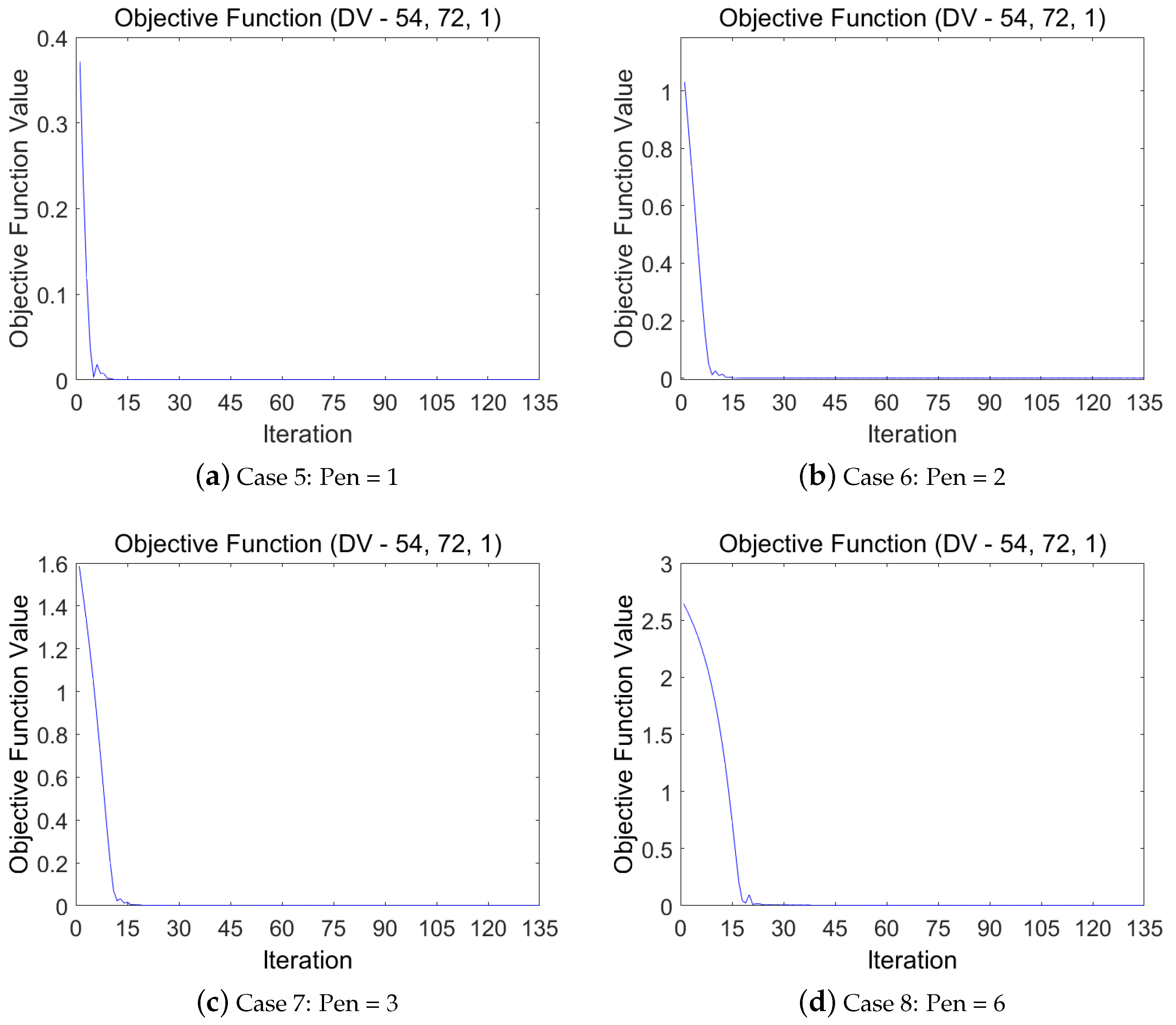
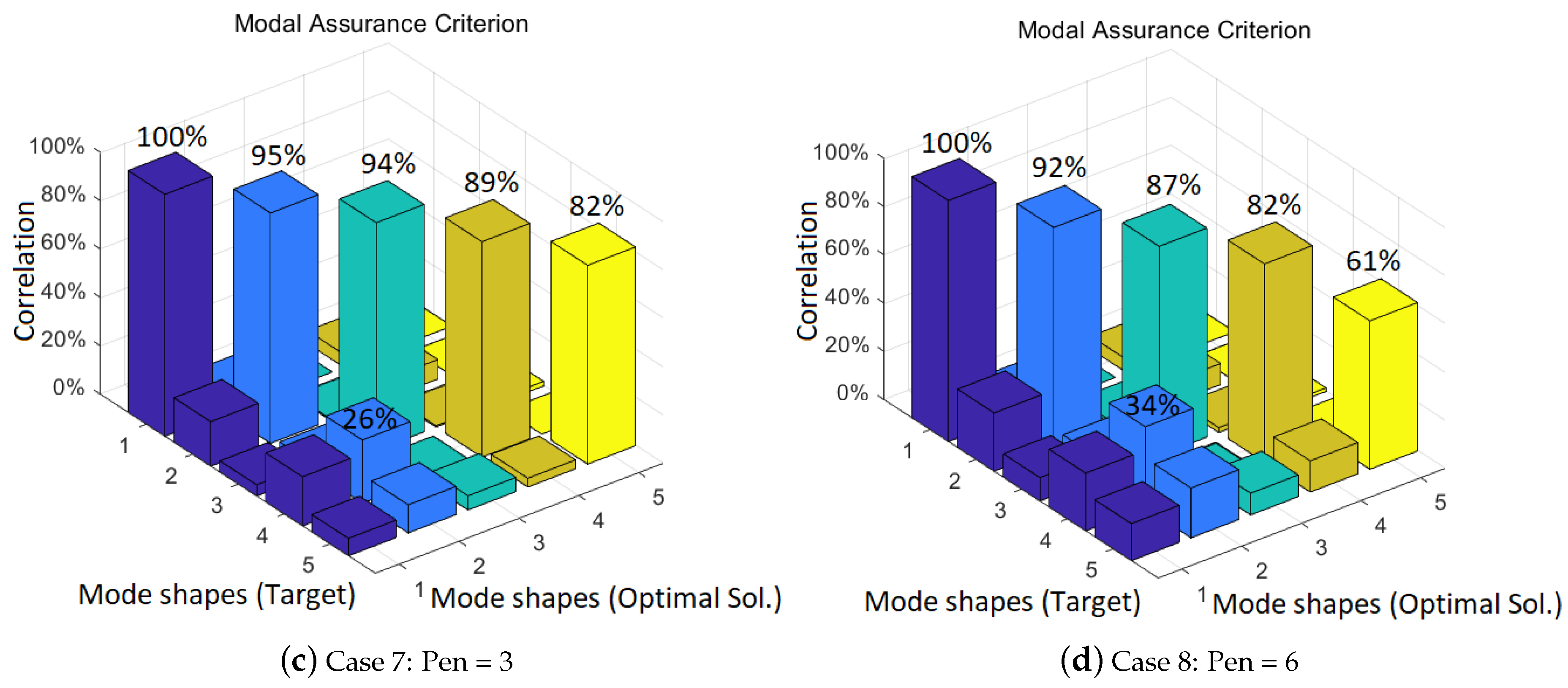
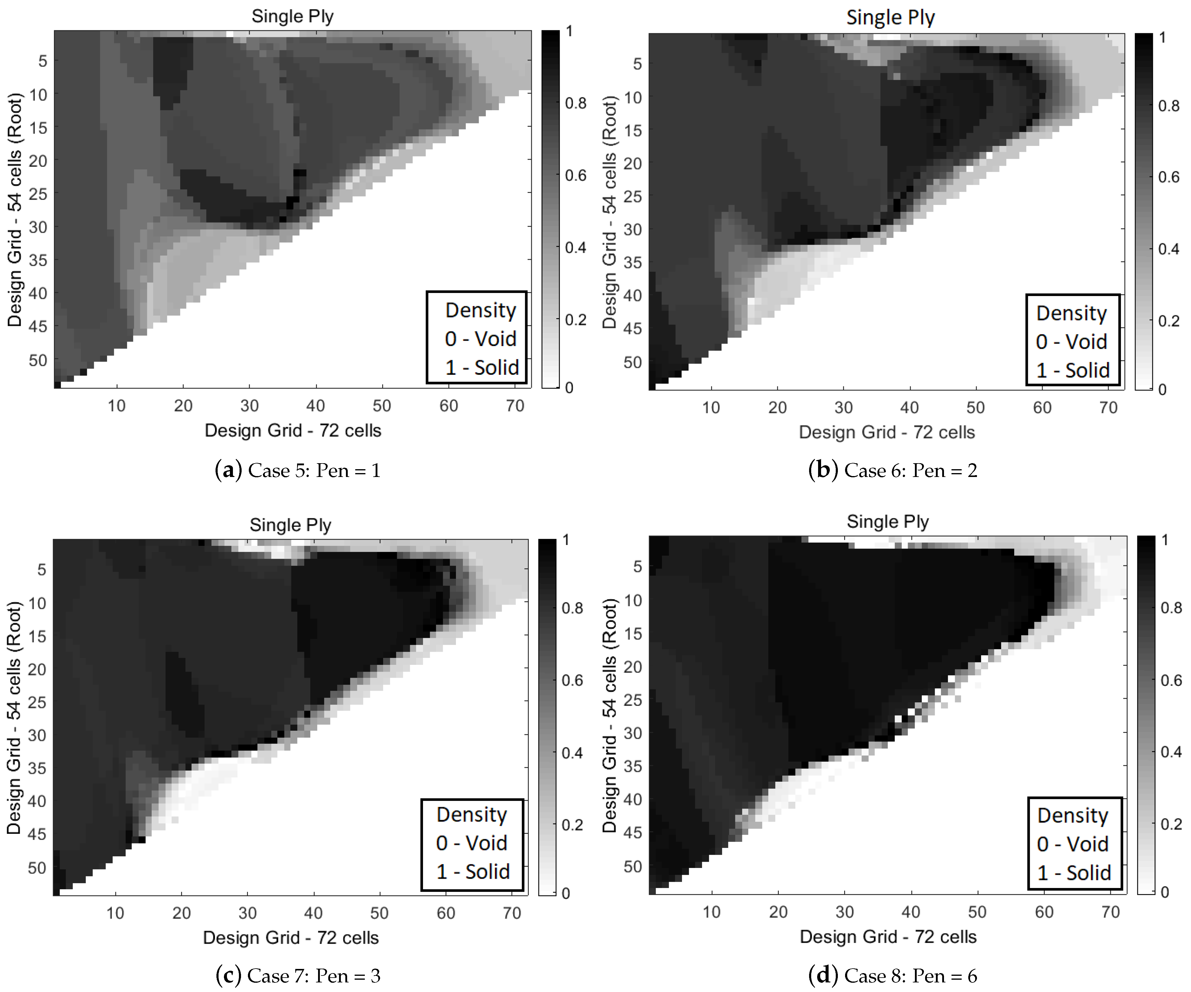
3.3. Penalization Factor Test Case

The penalization factor influence on the topologically optimized structures is now the focus of study in this test case. Four different penalization values are used for the finest considered design grid (54, 72, 1): 1 (Case 5), 2 (Case 6), 3 (Case 7) and 6 (Case 8). Despite the same full size model as for Cases 3 and 4 is used in these case studies, the materials and shell thickness of the scaled model are now different. The material properties of both models are summarized in Table 5. A Titanium alloy (Ti-6Al-4V (Grade 5)), often used for manufacturing through 3D printing [37], is considered for the internal part (solids A and B) of the scaled model. This pose an even higher challenged than before since the difference between properties increases. Regarding the shell, it is now 1 mm thick, i.e., equal to the full size model. This choice is related to the trend of reducing material near the root observed in Figure 12.
Given the high computational cost of these numerical optimizations, the maximum number of iterations is set to 135. A stable convergence history of the objective function can be seen in Figure 13 for the 4 considered penalization factors. As expected, the proposed dynamic scaling methodology takes more iterations to reduce the objective function when a higher penalization factor is considered since the design freedom is reduced. The lowest obtained objective function values are: 1.7412 × 10 4 at iteration 120 for Case 5; 6.1544 × 10 5 at iteration 128 for Case 6; 8.6974 × 10 5 at iteration 64 for Case 7; and 1.1874 × 10 3 at iteration 97 for Case 8.
These relatively low objective function values indicate that the first five natural frequencies are very close to the target ones, which is confirmed in Table 6. Even though higher objective function values and relative errors of frequencies are in general obtained by increasing the penalization factor, the relative errors are still low. In fact, the highest error (1.16%) is determined for the fifth vibration mode considering the highest penalization factor (Case 8). Thus, showing the proposed methodology effectiveness in matching the natural frequencies.
The correlation between target and scaled mode shapes is again assessed through the MAC metric, which is depicted in Figure 14 for the considered cases. This correlation is clearly observed to degrade as the penalization factor is increased. When using the lowest value (Case 5), a very good agreement between mode shapes is found since the lowest correlation is 94 % and the highest off-diagonal term is 16%, as illustrated in Figure 14a. Both these values are within the range usually deemed as acceptable, 80 % and 20 % for correlation and off-diagonal terms, respectively, [38]. By increasing the penalization factor to the double (Case 6, Figure 14b), despite an off-diagonal term of 24 % is calculated, the lowest correlation ( 91 % ) is still considerably higher than the above mentioned threshold. For this reason, Case 6 is still considered a good result by the authors. However, for the Case 7 (Figure 14c) these metrics continues degrading and the lowest correlation falls to 82 % , which is barely above the threshold value, but the maximum off-diagonal term slightly raises to 26 % . Given the fact that at least the correlation is still above the threshold value, this case is considered acceptable by the authors although not desirable. For Case 8 (Figure 14d) both these thresholds are not satisfied for the first five mode shapes, thus the mode shape matching is deemed not achieved even though the frequencies present low relative errors.
The topologically optimized internal structures for the different cases are shown in Figure 15. It is possible to identify areas with different intermediate density in all the cases. Despite increasing the penalization factor has not allowed for completely removing all intermediate densities, its amount has reduced. The identification of well-defined areas with intermediate densities makes the post-processing with different materials an attractive strategy. However, this approach might not be possible for other cases, e.g., the resulting intermediate material properties can be nonexistent. Furthermore, even if the second material exists it might not be compatible with the original one. Thus, a multi-material topology optimization can be a promising strategy for dynamic scaling.
The studies considering different penalties enabled important remarks. First, the increasing of the penalization negatively affected the quality of results in such a way that the optimizer failed in performing the matching of 5th mode shape for Case 8. The same effect was observed for the matching of the frequencies, although the worst result was 1.16 % which is fully accepted. Even the highest penalty factor not allowed achieving a gradient-free solution. However, observing how the penalty affected the results, a suitable solution of such optimization problems considering just gradient-free designs is really a very hard task. For instance, the matching of both natural frequencies and mode shapes with the same quality as reached with Pen = 1 maybe impossible to be achieved through a fully gradient-free approach.

4. Concluding Remarks

In this paper, a dynamic scaling methodology using topology optimization was introduced with the aim at designing scaled models that can be used to meaningfully evaluate unconventional designs for different engineering applications (e.g., aerospace, civil and mechanical engineering). Eight case studies of increasing difficulty were conducted to assess its effectiveness in representing the same dynamic behavior, in terms of natural frequencies and associated mode shapes, of a full size model in a reduced scale one. This methodology was found very promising in matching both the natural frequencies and modes shapes when the differences between material properties are small. The MAC metric was found to be close to an identity matrix and the relative difference between natural frequencies is under 1%. As these differences increase, even though the correlation between mode shapes from full and scaled models degrades (some diagonal terms become lower than 90%), a very good agreement was still reached. Nevertheless, the obtained solutions were characterized by presenting intermediate densities, even after increasing the design space, which are not suitable for additive manufacturing. Thus, a penalization factor was added to reduce these intermediate densities. When adding this factor, despite very low discrepancies were found for the frequencies (lower than 1.2 % ), the correlation between mode shapes noticeably degrades, with off-diagonal terms above 20% for penalization factors above 2. In fact, for the last considered case the thresholds usually deemed acceptable for the MAC metric were passed.
A solution that could mitigate this issue is using a multi-material topology optimization strategy for the dynamic scaling process. Alternatively, the MAC metric could be included in the objective function, while accounting for manufacturing feasibility constraints.

Author Contributions

Conceptualization, É.O., A.S. (Abdolrasoul Sohouli), F.A., R.G.A.d.S. and A.S. (Afzal Suleman); methodology, É.O., A.S. (Abdolrasoul Sohouli) and F.A.; software, É.O. and A.S. (Abdolrasoul Sohouli); validation, É.O. and A.S. (Abdolrasoul Sohouli); formal analysis, É.O.; investigation, É.O.; data curation, É.O.; writing—original draft preparation, É.O. and F.A.; writing—review and editing, A.S. (Afzal Suleman); visualization, É.O.; supervision, R.G.A.d.S. and A.S. (Afzal Suleman); project administration, A.S. (Afzal Suleman). All authors have read and agreed to the published version of the manuscript.

Funding

The authors acknowledge Fundação para a Ciência e a Tecnologia (FCT), through IDMEC, under LAETA, project UIDB/50022/2020. É.O. acknowledges the support received from the Brazilian Research Agency CNPq through the INCT-EIE, (Proj. 400211/2012-2, Proc. 229039/2013-8).

Informed Consent Statement

Not applicable.

Data Availability Statement

The new data presented in this study is available on request.

Conflicts of Interest

The authors declare no conflict of interest.

References

  1. Okonkwo, P.; Smith, H. Review of evolving trends in blended wing body aircraft design. Prog. Aerosp. Sci. 2016, 82, 1–23. [Google Scholar] [CrossRef]
  2. Cavallaro, R.; Demasi, L. Challenges, Ideas, and Innovations of Joined-Wing Configurations: A Concept from the Past, an Opportunity for the Future. Prog. Aerosp. Sci. 2016, 87, 1–93. [Google Scholar] [CrossRef]
  3. Papageorgiou, A.; Tarkian, M.; Amadori, K.; Ölvander, J. Multidisciplinary Design Optimization of Aerial Vehicles: A Review of Recent Advancements. Int. J. Aerosp. Eng. 2018, 2018, 4258020. [Google Scholar] [CrossRef]
  4. Zhu, W. Models for wind tunnel tests based on additive manufacturing technology. Prog. Aerosp. Sci. 2019, 110, 100541. [Google Scholar] [CrossRef]
  5. Sobron, A.; Lundström, D.; Krus, P. A Review of Current Research in Subscale Flight Testing and Analysis of Its Main Practical Challenges. Aerospace 2021, 8, 74. [Google Scholar] [CrossRef]
  6. Casaburo, A.; Petrone, G.; Franco, F.; De Rosa, S. A Review of Similitude Methods for Structural Engineering. Appl. Mech. Rev. 2019, 71, 030802. [Google Scholar] [CrossRef] [Green Version]
  7. Georgiou, G.; Vio, G.A.; Cooper, J.E. Aeroelastic tailoring and scaling using Bacterial Foraging Optimisation. Struct. Multidiscip. Optim. 2014, 50, 81–99. [Google Scholar] [CrossRef]
  8. He, S.; Guo, S.; Liu, Y.; Luo, W. Passive gust alleviation of a flying-wing aircraft by analysis and wind-tunnel test of a scaled model in dynamic similarity. Aerosp. Sci. Technol. 2021, 113, 106689. [Google Scholar] [CrossRef]
  9. Bond, V.L.; Canfield, R.A.; Suleman, A.; Blair, M. Aeroelastic Scaling of a Joined Wing for Nonlinear Geometric Stiffness. AIAA J. 2012, 50, 513–522. [Google Scholar] [CrossRef]
  10. Wan, Z.; Cesnik, C.E.S. Geometrically Nonlinear Aeroelastic Scaling for Very Flexible Aircraft. AIAA J. 2014, 52, 2251–2260. [Google Scholar] [CrossRef] [Green Version]
  11. Ricciardi, A.P.; Canfield, R.A.; Patil, M.J.; Lindsley, N. Nonlinear Aeroelastic Scaled-Model Design. J. Aircr. 2016, 53, 20–32. [Google Scholar] [CrossRef]
  12. Mas Colomer, J.; Bartoli, N.; Lefebvre, T.; Martins, J.R.R.A.; Morlier, J. An MDO-based methodology for static aeroelastic scaling of wings under non-similar flow. Struct. Multidiscip. Optim. 2021, 63, 1045–1061. [Google Scholar] [CrossRef]
  13. Spada, C.; Afonso, F.; Lau, F.; Suleman, A. Nonlinear aeroelastic scaling of high aspect-ratio wings. Aerosp. Sci. Technol. 2017, 63, 363–371. [Google Scholar] [CrossRef]
  14. Afonso, F.; Coelho, M.; Vale, J.; Lau, F.; Suleman, A. On the Design of Aeroelastically Scaled Models of High Aspect-Ratio Wings. Aerospace 2020, 7, 166. [Google Scholar] [CrossRef]
  15. Wang, G.; Zhang, M.; Tao, Y.; Li, J.; Li, D.; Zhang, Y.; Yuan, C.; Sang, W.; Zhang, B. Research on analytical scaling method and scale effects for subscale flight test of blended wing body civil aircraft. Aerosp. Sci. Technol. 2020, 106, 106114. [Google Scholar] [CrossRef]
  16. Banazadeh, A.; Hajipouzadeh, P. Using approximate similitude to design dynamic similar models. Aerosp. Sci. Technol. 2019, 94, 105375. [Google Scholar] [CrossRef]
  17. French, M.; Eastep, F.E. Aeroelastic model design using parameter identification. J. Aircr. 1996, 33, 198–202. [Google Scholar] [CrossRef]
  18. Stanford, B. Topology Optimization of Low-Speed Aeroelastic Wind Tunnel Models. AIAA Scitech 2021 Forum 2021. [Google Scholar] [CrossRef]
  19. Bendsøe, M.P.; Kikuchi, N. Generating optimal topologies in structural design using a homogenization method. Comput. Methods Appl. Mech. Eng. 1988, 71, 197–224. [Google Scholar] [CrossRef]
  20. Zhu, J.H.; Zhang, W.H.; Xia, L. Topology Optimization in Aircraft and Aerospace Structures Design. Arch. Comput. Methods Eng. 2016, 23, 595–622. [Google Scholar] [CrossRef]
  21. Meng, L.; Zhang, W.; Quan, D.; Shi, G.; Tang, L.; Hou, Y.; Breitkopf, P.; Zhu, J.; Gao, T. From Topology Optimization Design to Additive Manufacturing: Today’s Success and Tomorrow’s Roadmap. Arch. Comput. Methods Eng. 2020, 27, 805–830. [Google Scholar] [CrossRef]
  22. Goh, G.; Agarwala, S.; Goh, G.; Dikshit, V.; Sing, S.; Yeong, W. Additive manufacturing in unmanned aerial vehicles (UAVs): Challenges and potential. Aerosp. Sci. Technol. 2017, 63, 140–151. [Google Scholar] [CrossRef]
  23. Klippstein, H.; Diaz De Cerio Sanchez, A.; Hassanin, H.; Zweiri, Y.; Seneviratne, L. Fused Deposition Modeling for Unmanned Aerial Vehicles (UAVs): A Review. Adv. Eng. Mater. 2018, 20, 1700552. [Google Scholar] [CrossRef] [Green Version]
  24. Liu, J.; Gaynor, A.T.; Chen, S.; Kang, Z.; Suresh, K.; Takezawa, A.; Li, L.; Kato, J.; Tang, J.; Wang, C.C.L.; et al. Current and future trends in topology optimization for additive manufacturing. Struct. Multidiscip. Optim. 2018, 57, 2457–2483. [Google Scholar] [CrossRef] [Green Version]
  25. Allaire, G.; Dapogny, C.; Estevez, R.; Faure, A.; Michailidis, G. Structural optimization under overhang constraints imposed by additive manufacturing technologies. J. Comput. Phys. 2017, 351, 295–328. [Google Scholar] [CrossRef] [Green Version]
  26. Lazarov, B.S.; Wang, F.; Sigmund, O. Length scale and manufacturability in density-based topology optimization. Arch. Appl. Mech. 2016, 86, 189–218. [Google Scholar] [CrossRef] [Green Version]
  27. Gaynor, A.T.; Guest, J.K. Topology optimization considering overhang constraints: Eliminating sacrificial support material in additive manufacturing through design. Struct. Multidiscip. Optim. 2016, 54, 1157–1172. [Google Scholar] [CrossRef]
  28. Deaton, J.D.; Kolonay, R.M.; Reuter, R.A.; Kobayashi, M.H. Validation of Topology Optimized Lifting Surfaces using 3-D Printing. In Proceedings of the 17th International Forum on Aeroelasticity and Structural Dynamics (IFASD), Como, Italy, 25–28 June 2017. [Google Scholar]
  29. Pastor, M.; Binda, M.; Harčarik, T. Modal Assurance Criterion. Procedia Eng. 2012, 48, 543–548. [Google Scholar] [CrossRef]
  30. Stolpe, M.; Svanberg, K. An alternative interpolation scheme for minimum compliance optimization. Struct. Multidiscip. Optim. 2001, 22, 116–124. [Google Scholar] [CrossRef]
  31. Bendsøe, M.P. Optimal shape design as a material distribution problem. Struct. Optim. 1989, 1, 193–202. [Google Scholar] [CrossRef]
  32. Tsai, T.; Cheng, C.C. Structural design for desired eigenfrequencies and mode shapes using topology optimization. Struct. Multidiscip. Optim. 2001, 47, 673–686. [Google Scholar] [CrossRef]
  33. Wächter, A.; Biegler, L.T. On the implementation of an interior-point filter line-search algorithm for large-scale nonlinear programming. Math. Program. 2006, 106, 25–57. [Google Scholar] [CrossRef]
  34. MatWeb, Material Property Data. Property Search. Available online: http://www.matweb.com/search/PropertySearch.aspx (accessed on 21 May 2021).
  35. Silva, M.; Mateus, A.; Oliveira, D.; Malça, C. An alternative method to produce metal/plastic hybrid components for orthopedics applications. Proc. Inst. Mech. Eng. Part J. Mater. Des. Appl. 2017, 231, 179–186. [Google Scholar] [CrossRef]
  36. Zhan, J.; Tamura, T.; Li, X.; Ma, Z.; Sone, M.; Yoshino, M.; Umezu, S.; Sato, H. Metal-plastic hybrid 3D printing using catalyst-loaded filament and electroless plating. Addit. Manuf. 2020, 36, 101556. [Google Scholar] [CrossRef]
  37. Chen, L.; Huang, J.; Lin, C.; Pan, C.; Chen, S.; Yang, T.; Lin, D.; Lin, H.; Jang, J. Anisotropic response of Ti-6Al-4V alloy fabricated by 3D printing selective laser melting. Mater. Sci. Eng. A 2017, 682, 389–395. [Google Scholar] [CrossRef]
  38. Ewins, D.J. Modal Testing: Theory, Practice and Application, 2nd ed.; John Wiley & Sons: Baldock, UK, 2009. [Google Scholar]
Figure 1. Dynamic scaling methodology.
Machines 10 00374 g001
Figure 2. Full scale model: (a) dimensions and material application; (b) internal structure-solid model; (c) external surface-shell model (2 faces).
Machines 10 00374 g002
Figure 3. Full scale model—boundary condition.
Machines 10 00374 g003
Figure 4. Mesh convergence study for the solid model.
Machines 10 00374 g004
Figure 5. Design grid for the two considered meshes, where (X, Y, Z) denote the number of cells in x, y and z planes.
Machines 10 00374 g005
Figure 6. Objective function convergence for Cases 1 and 2.
Machines 10 00374 g006
Figure 7. Modal Assurance Criterion for Cases 1 and 2.
Machines 10 00374 g007
Figure 8. Topology optimization solutions of Cases 1 and 2.
Machines 10 00374 g008
Figure 9. Objective function convergence for Cases 3 and 4.
Machines 10 00374 g009
Figure 10. Modal Assurance Criterion for Cases 3 and 4.
Machines 10 00374 g010
Figure 11. Topology optimization solutions of Cases 3 and 4.
Machines 10 00374 g011
Figure 12. Topology optimization solutions of Cases 3 with and without post-processing.
Machines 10 00374 g012
Figure 13. Objective function convergence for Cases 5, 6, 7 and 8.
Machines 10 00374 g013
Figure 14. Modal Assurance Criterion for Cases 5, 6, 7 and 8.
Machines 10 00374 g014aMachines 10 00374 g014b
Figure 15. Dynamically Scaled structure-Comparison about penalization factor (Pen = 1, 2, 3 and 6) using no projection filter.
Machines 10 00374 g015
Table 1. Comparison between the material properties of the target and scaled models for Cases 1 and 2.
Case 1Case 2
Material PropertyTargetScaled ModelDifference [%]TargetScaled ModelDifference [%]
Density ρ [ kg / m 3 ] 24002700112400270011
Part-1, Solid AElasticity modulus E [ Pa ] 60 × 10 9 70 × 10 9 14 60 × 10 9 70 × 10 9 14
Poisson Ratio ν [ ] 0.330.3090.330.309
Density ρ [ kg / m 3 ] 22002700192000270026
Part-1, Solid BElasticity modulus E [ Pa ] 66 × 10 9 70 × 10 9 6 55 × 10 9 70 × 10 9 21
Poisson Ratio ν [ ] 0.360.30170.360.3017
Density ρ [ kg / m 3 ] 22001800181210180033
Part-2, ShellElasticity modulus E [ Pa ] 66 × 10 9 40 × 10 9 39 66 × 10 6 40 × 10 9 60,506
Poisson Ratio ν [ ] 0.360.3380.360.338
Table 2. Comparison between the target frequencies and obtained ones for Cases 1 and 2. F denotes frequency.
Case 1Case 2
Target F [Hz]Obtained F [Hz]Relative Error [%]Target F [Hz]Obtained F [Hz]Relative Error [%]
Mode 161.0061.060.0159.2458.900.06
Mode 2263.77264.760.04257.61257.540.00
Mode 3378.81381.530.07368.66368.770.00
Mode 4656.28655.540.01643.87640.550.05
Mode 5918.68917.470.01897.06891.730.06
Table 3. Comparison between the material properties of the target and scaled models for Cases 3 and 4.
TargetScaled ModelDifference [%]
Density ρ [ kg / m 3 ] 2400270013
Part-1, Solid AElasticity modulus E [ Pa ] 60 × 10 9 70 × 10 9 17
Poisson ν [ ] 0.330.309
Density ρ [ kg / m 3 ] 1800270050
Part-1, Solid BElasticity modulus E [ Pa ] 30 × 10 9 70 × 10 9 133
Poisson ν [ ] 0.360.3017
Density ρ [ kg / m 3 ] 1210180049
Part-2, ShellElasticity modulus E [ Pa ] 66 × 10 6 40 × 10 9 60,506
Poisson ν [ ] 0.360.338
Table 4. Comparison between the target frequencies and obtained ones for Cases 3 and 4. F denotes frequency.
Case 3Case 4
Target F [Hz]Obtained F [Hz]Relative Error [%]Obtained F [Hz]Relative Error [%]
Mode 152.3152.720.8751.940.71
Mode 2234.32235.430.47235.510.50
Mode 3321.93324.670.85321.070.27
Mode 4592.69595.440.46593.840.19
Mode 5786.21785.530.09791.050.61
Table 5. Comparison between the material properties of the target and scaled models for Cases 5, 6, 7 and 8.
TargetScaled ModelDifference [%]
Density ρ [ kg / m 3 ] 2400443046
Part-1, Solid AElasticity modulus E [ Pa ] 60 × 10 9 113.8 × 10 9 47
Poisson ν [ ] 0.330.3424
Density ρ [ kg / m 3 ] 1800443059
Part-1, Solid BElasticity modulus E [ Pa ] 30 × 10 9 113.8 × 10 9 74
Poisson ν [ ] 0.360.3425
Density ρ [ kg / m 3 ] 121012100
Part-2, ShellElasticity modulus E [ Pa ] 66 × 10 6 66 × 10 6 0
Poisson ν [ ] 0.360.338
Table 6. Comparison between the target frequencies and obtained ones for Cases 5, 6, 7 and 8. F denotes frequency. The errors are relative to the target.
Case 5: Pen = 1Case 6: Pen = 2Case 7: Pen = 3Case 8: Pen = 6
TargetObtainedRelativeObtainedRelativeObtainedRelativeObtainedRelative
NF [Hz]F [Hz]Error [%]F [Hz]Error [%]F [Hz]Error [%]F [Hz]Error [%]
Mode 152.3152.580.5252.470.3152.420.2152.670.68
Mode 2234.32234.610.12234.670.15234.870.23236.630.98
Mode 3321.93322.790.27322.470.17322.610.21323.220.40
Mode 4592.69591.370.22592.270.07593.740.18592.330.06
Mode 5786.21787.460.16786.570.04787.840.21795.341.16
Publisher’s Note: MDPI stays neutral with regard to jurisdictional claims in published maps and institutional affiliations.

