Abstract
The scale of offshore wind turbines (OWTs) has increased in order to enhance their energy generation. However, strong aero/hydrodynamic loads can degrade the dynamic characteristics of OWTs because they are installed on soft seabeds. This degradation can shorten the structural life of the system; repetitive loads lead to seabed softening, reducing the natural frequency of the structure close to the excitation frequency. Most of the previous studies on degradation trained prediction algorithms with actual sensor signals. However, there are no actual sensor data on the dynamic response of OWTs over their lifespan (approximately 20 years). In order to address this data issue, this study proposes a new prediction platform combining a dynamic OWT model and a neural network-based degradation prediction model. Specifically, a virtual dynamic response was generated using a three-dimensional OWT and a seabed finite element model. Then, the LSTM model was trained to predict the natural frequency degradation using the dynamic response as the model input. The results show that the developed model can accurately predict natural frequencies over the next several years using past and present accelerations and strains. In practice, this LSTM model could be used to predict future natural frequencies using the dynamic response of the structure, which can be measured using actual sensors (accelerometers and strain gauges).
1. Introduction
Offshore wind turbines (OWTs) are subjected to strong wind and oscillating waves. The rotation of the blades leads to thrust force on the tower of the OWTs [1], and the wave exerts hydrodynamic loads on the offshore platform [2]. Additionally, atmospheric turbulence, turbulent air flows, non-steady flow at the blades, and blade-generating turbulence also affect the dynamic response of the OWTs [3,4]. The abovementioned loads result in the vibration of the OWTs, which is transferred to the soil in which the structure is constructed. This cyclic load can change the modulus of the soil [5]. Consequently, the system’s NF resonates with the blade rotational frequencies, increasing the possibility of fatal effects on the remaining lifespan of the system [6].
Previous studies have shown that predicting the dynamic behavior of OWTs is important and necessary in order to prevent resonance. The US National Renewable Energy Laboratory provides multiple open-source simulation models [7]. Moreover, many studies have attempted to verify a fully coupled simulation model using OWTs and a soil model. Long-term OWT simulation models have made significant advances [8,9,10]. They can optimize design parameters using simulation results or predict the dynamic behavior, which changes as the soil foundation degrades. Accordingly, it is necessary to build a long-term OWT simulation model in order to predict collapses and design appropriate repair strategies. The OWT maintenance and repair costs can be reduced if the collapse of the entire system due to soil degradation can be predicted. Remaining useful life (RUL) prediction for structural systems is important in order to reduce maintenance costs and improve system reliability, while also playing a vital role in scheduling and condition-based decision-making.
Degradation prediction methods can be divided into three main categories: model-based, data-driven, and hybrid methods. Model-based methods create mathematical models to describe the degradation of systems or components (e.g., the Eyring model [11], particle filters [12], and Weibull distribution [13]). They can provide accurate predictions if the model is developed with extensive knowledge of the degradation mechanisms of the systems. However, it is difficult to establish a precise mathematical or physical model for complex systems under various conditions [14]. Moreover, they incur a high computational cost because of the complex dynamic system under complex wind and wave conditions. Data-driven methods use sensor data for prediction. Compared to model-based methods, data-driven methods do not require significant prior knowledge regarding the physical system, and can be easily generated. Considering the developments in data analysis techniques, various deep learning models have been applied to data-driven approaches. Ren et al. [15] suggested a deep neural network model for rolling bearing degradation prediction. Li et al. [16] developed deep convolution neural networks for aero-engine degradation using the publicly available C-MAPSS dataset. Zhou et al. [17] proposed a prediction model for supercapacitors with a long short-term memory network (LSTM). However, data-driven methods require a large amount of data. Therefore, a hybrid method was proposed in order to overcome the limitations of model-based and data-driven methods. In particular, using physically model-simulated data as the input to a data-driven method, the hybrid method can predict degradation with only a small amount of data. Cai et al. [18] proposed a hybrid approach for sub-sea pipelines in offshore oil and gas production systems. Feng et al. [19,20] developed a hybrid model for mechanical gear degradation. They first designed a dynamic model and a fatigue model of a spur gear system. Then, the degradation parameter on the gear was updated over the long cycles using the experimentally measured vibration signals.
In this study, a hybrid method was developed to predict the dynamic behavior of a tripod OWT. A long-term OWT simulation model was developed to generate time-varying dynamic behavior data over the desired life span of the tripod OWT (i.e., 20 years). First, a finite element model (FEM) was built using a 3-MW WinDS3000 TC-2 wind turbine (Doosan Heavy Industries & Construction, Changwon, Korea) [21] installed in the southwestern sea region of the Korean Peninsula. This model was used to calculate the dynamic behavior of the tripod OWT. Then, the OWT model parameters were determined using the sensor data from the actual structure. Next, the long-term virtual sensor data of the OWT were obtained using the FEM, and the acceleration, strain, and NF of the OWT structure were collected. It is challenging to acquire actual long-term OWT sensor data because most OWTs have only recently been installed. Alternatively, virtual data were obtained from the model, and such data were used to train the OWT NF degradation prediction model. Subsequently, the performance of the prediction model was validated using a test dataset.
The remainder of this paper is organized as follows. Section II describes the FEM and soil modulus degradation model. Section III describes the data generation method using the model presented in Section II. Section IV describes the LSTM model for NF prediction and its test results. Finally, Section V summarizes and concludes this paper.
2. OWT and Seabed Dynamic Model
OWT sensor data are required over its lifespan (i.e., 20 years) to train the NF degradation prediction model. However, collecting 20-year data from the OWT is difficult because most offshore wind farms have been recently constructed. Thus, this study calculated virtual sensor data from a physical model of the OWT, seabed, and aero/hydrodynamic loads. The prediction model was then trained and validated using the virtual sensor data.
In this section, the integrated physical OWT model is described. Section 2.1 presents the dimensions and mechanical properties of the OWT structure and seabed. In Section 2.2, the model parameter values are determined using structural health monitoring data. Section 2.3 describes the mathematical soil degradation model.
2.1. Three-Dimensional Finite Element Model
A three-dimensional FEM was built using a 3-MW WinDS3000 TC-2 wind turbine with a tripod substructure, as shown in Figure 1. Triangular shell elements were used for the tower, substructure, and suction buckets. The weight of the rotor-nacelle assembly (RNA) is 186 t; the nacelle, hub, and blades are 128, 28, and 28 t, respectively. The diameter of the blades is 100 m [21]. This turbine assembly is considered to have a lumped mass, and is located at the top of the wind tower. The dimensions of the structure, with suction buckets supporting the wind turbine, are listed in Table 1 [21]. The properties of the steel used for the tower, substructure, and suction buckets are listed in Table 2 [21]. The mean sea water level was set at 13.6 m.
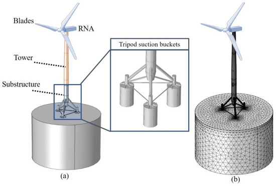
Figure 1.
OWT system comprising the OWT structure and soil. (a) OWT components; (b) 3D FEM mesh model.

Table 1.
OWT model dimensions.
Table 2.
Properties of the steel used for the OWT.
The soil model was established using soil data obtained from standard penetration and cone penetration tests; the soil properties were measured at 35°58′19.43″ N latitude and 126°30′53.39″ E longitude [21]. The seabed consists of three layers, and the soil properties were determined as shown in Table 3. Previous studies have shown that a soil finite model provides reliable results when its diameter is six times larger than the suction caisson diameter and its length is 3.5 times longer than the suction caisson length [22,23]. Therefore, the size of the soil model in this study was determined using these criteria.
Table 3.
Soil properties.
2.2. Damping Ratio
The total damping of the entire OWT system depends on several damping sources [24]: structural, aerodynamic, hydrodynamic, and soil damping. A damping ratio of 2–3% is typically used to describe the overall damping effect for OWTs [25,26,27].
The overall damping ratio can be determined using the initial NF of the OWT. The NF of the actual OWT was measured over four installation stages, as shown in Figure 2a1–a4 [21]. The substructure, including the suction caissons, was installed in Stage I. The bottom and middle towers were installed in Stage II. In Stage III, the remaining part of the tower was assembled and the nacelle was installed. The hub and blades were assembled in Stage IV. The NF was measured using accelerometers attached to the structure [21].
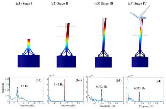
Figure 2.
Dynamic response of the OWT for different installation stages. (a1–a4) First mode shape of the OWT for Stages I–IV; (b1–b4) Frequency response of the accelerometers for Stages I–IV; the NF of each stage is indicated within the corresponding panel.
The NF of Stage I was obtained using an accelerometer signal impact test [21]. Accelerometers were attached to the transition piece of the tower and substructure in order to acquire the acceleration data. The NFs of Stages I–IV were determined to be 3.2, 1.42, 0.372, and 0.323 Hz, respectively, as shown in Figure 2b1–b4. The overall damping ratio of the FEM was set as 2% because this value accurately calculates the NFs; the NF errors were 0.18%, 1.4%, 0.9%, and 0.05% for Stages I–IV, respectively.
2.3. Soil Degradation Model
Wind- and wave-generated stochastic loads degrade the soil modulus. This degradation was calculated for all of the nodes in the seabed. A frequency-domain analysis was used to reduce the computational cost, as opposed to a time-domain analysis. Stochastic soil stress variations can be considered via Rayleigh and Gaussian distributions [28]. Based on these probabilistic properties, Nam et al. [28] proposed a method to rapidly calculate stochastic soil stress variations without using the Monte Carlo method. They also proposed a soil degradation calculation method in the presence of stochastically fluctuating stress. We adopted the above-mentioned methods for the FEM in order to calculate the soil modulus degradation under different wind conditions.
The degradation function parameters must be determined before applying the previous degradation model [28] to the OWT model. In this study, the degradation function , which describes the degradation ratio using the normalized shear stress amplitude and normalized shear stress mean , is described as
where N is the number of repetitive loading cycles applied to the soil. Parameters , , and determine the degradation speed. This empirical relation was obtained using previous stress-controlled cyclic load test results for soil [29]. The values of , , and were determined based on experimental data. In this study, were randomly determined as 0.07, 2.24, and 11.78, respectively.
3. Virtual Sensor Data Generation
The virtual sensor data were measured for 14 different locations based on ten accelerometers and four strain gauges attached to the 3-MW WinDS3000 TC-2 turbine.
3.1. Wind Conditions
When the OWT blades are rotated by the wind, a thrust force is also applied to the rotor axis. The thrust force magnitude is calculated as follows:
where is the air density, is the blade radius, is the wind speed at hub height, and is the thrust coefficient. The air density was 1.252 kg/m3 at the candidate site [30]. The blade radius is 45.6 m, and thrust coefficient —which varies according to wind speed—for the WinDS3000 TC-2 turbine was provided by Doosan Heavy Industries & Construction [28]. The stochastic wind speed was obtained from the Kaimal spectrum, as described in [30]. The wave-caused dynamic pressure should be considered to predict the dynamic response of the structure and soil. The stochastic wave elevation was obtained from Pierson and Moskowitz [30], which describes the wave power spectrum as a function of wind speed. The pressure applied to the submerged part of the structure by a wave can be calculated using potential theory [28]. Once the wind speed is determined, the aero/hydrodynamic loads are determined.
The Weibull distribution shape and scale parameters (k and c, respectively) were used for the wind speed probability. In order to consider various wind speed conditions, virtual sensor signals were obtained for nine different sets of (k, c) = (5.27, 4.50), (6.3, 4.7), (6.02, 1.78), (7.53, 1.83), (12.8, 8.0), (13.55, 2.12), (17.02, 6.0), (15.52, 5.02), and (18.1, 9.0), as shown in Figure 3. Note that the values of c and k for wind speed distribution are approximately 7.5 and 1.8, respectively, in the southwestern sea of the Korean Peninsula [31]. Thus, the values of the c and k of this study were determined such that the order of the value is similar to that of the experimental data. The purpose of this study is to establish the NF prediction model, and to verify its performance under various conditions. Thus, the values of c and k significantly vary in order to consider various wind conditions, and to check if the proposed model can predict the NF in the various wind conditions. However, when this model is applied to a specific wind farm, the exact c and k values of the site need to be considered.
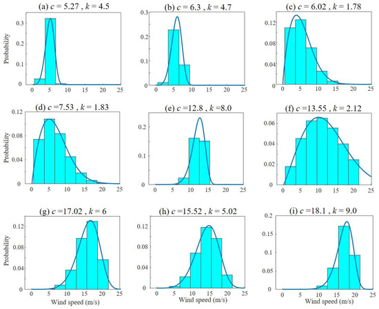
Figure 3.
Probability distribution obtained using the Weibull distribution parameters for nine different wind conditions.
3.2. Long-Term Structural Data
Long-term simulations were conducted using the FEM and the different wind distributions in order to acquire the virtual sensor dataset. The simulations were performed for the lifespan of the OWT (i.e., 20 years). The acceleration and strain frequency response functions (at 14 different positions) were acquired; these data correspond to the sensor data. The data were stored every 0.1 years; thus, a total of 200 samples were obtained for a 20-year simulation for a specific (k, c) set.
Figure 4 shows the NF over the long-term simulations. Nine different wind distributions, as described in Section 3.1, were applied to the OWT. As the wave model is a function of wind speed, the wave condition also changes as the wind distribution changes.
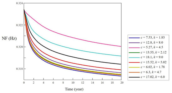
Figure 4.
Long-term (20 years) simulation results for various wind distributions.
4. NF Degradation Prediction
OWTs are subjected to strong wind and wave loads. Cyclical dynamic loading can change the modulus of the soil in which the structure is constructed. Soil modulus degradation changes the dynamic behavior of the OWT system, including the OWT and soil. For example, when the soil modulus decreases, the NF of the OWT system also decreases. This NF degradation can be critical for structural safety because the NF of the system is close to the rotating frequency of the blades. Thus, an NF prediction model was developed to prevent resonance.
4.1. LSTM for the Future NF
Among the nine wind distributions described in Section 3.1, the data corresponding to six distributions were used to train the LSTM model, and the remaining three distributions were used to validate its prediction performance. z-score normalization was applied in order to reduce the range difference between each feature. In this study, the LSTM model was designed to predict a three-year NF degradation using six-year virtual sensor data and wind speed as inputs.
The prediction model inputs and outputs are shown in Figure 5. The input comprised 22 signals over 60 stamps. This study used a 0.1-year time interval; thus, 60 time stamps correspond to a six-year span. The 22 signals are as follows: the wind speed Weibull distribution parameters k and c, the NF, the difference between NF and initial NF, the acceleration amplitudes at the NF (from ten accelerometer signals), the strain amplitudes at zero frequency (from four strain gauges), and the strain amplitudes at the NF (from four strain gauges). The output is the NF over three years (i.e., 30 time stamps).
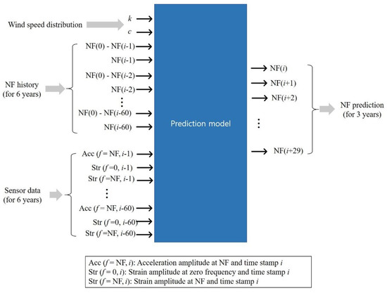
Figure 5.
Established OWT NF prediction model. The model inputs consist of six-year virtual sensor data and the wind speed Weibull distribution parameters; the model output consists of a three-year NF prediction.
The prediction model consists of a single LSTM layer and three dense layers, as shown in Figure 6. A hyperband [1] tuner was used to determine the optimal number of LSTM units and dense layer neurons. The hyperband tuner determined 75 LSTM units and 64, 448, and 512 neurons in each subsequent dense layer. A hyperbolic tangent was used as the activation function. Dropout layers were used with a dropout rate of 0.3 in order to increase the model generalization and avoid overfitting. The mean absolute error of NF was used as a loss function for training. The Adam optimizer with mini-batches was used. The maximum number of training epochs was set to 35,000, and a learning rate of 0.001 was used for the entire training epoch.
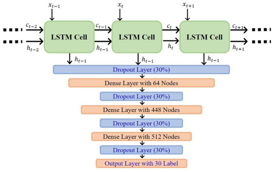
Figure 6.
Established LSTM model structure with one LSTM layer and three dense layers.
4.2. Prediction Results
The LSTM model performance was validated under three different wind distributions. Figure 7 shows two three-year degradation prediction examples in which the previous six-year data were used as the input. Figure 7a1–a3 shows the prediction results for 6–9 years when (k, c) = (12.8, 8.0) (Case A). Figure 7b1–b3 shows the prediction results for 12–15 years when (k, c) = (17.02, 6.0) (Case C). These results suggest that the model can predict the NF degradation trends; however, it produces some errors. One might argue that the NF degradation can be predicted with a simple curve fitting. However, the curve fitting approach is not suitable for this application because it cannot consider the temporal variation of the wind condition. Although the present work considers constant c and k values for the wind condition, the proposed model is able to consider temporally varying c and k; it can be trained if a new dataset with varying c and k is provided. Indeed, the development of a prediction model under time-varying wind conditions is a potential future work. However, the curve fitting approach cannot deal with the time-varying c and k.
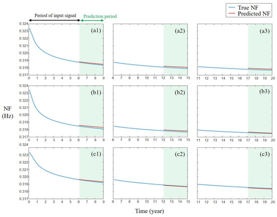
Figure 7.
NF prediction examples for different test datasets. Each result shows a degradation tendency for a three-year period using the previous six-year data as the input. (a1–a3), (b1–b3) and (c1–c3) represent results corresponding to Cases A, B, and C, respectively.
The prediction results were further investigated by calculating the absolute prediction error (%) for each test case for different three-year periods, as shown in Table 4. These results suggest the following model characteristics. First, a more dramatic NF degradation leads to a larger error. The NF of Cases A and B decreases rapidly compared to that of Case C. Moreover, the average error of Cases A and B is more than twice as large as that of Case C, suggesting that NF prediction is more challenging when intensive soil softening occurs. Second, a non-linear NF leads to a larger error. In Cases A and B, the NF prediction between 7 and 12 years had the largest error, while in Case C, the NF prediction for 6–9 years yielded the largest error. Figure 4 shows that the NF degradation in these periods is highly non-linear compared to other periods. Furthermore, Case C converges faster to a linear form than Cases A and B; thus, it exhibits the largest error in the initial period. As the proposed LSTM model does not have a deep structure, it has difficulties learning this complex non-linearity. The error could be reduced if the model is developed with a deeper structure.
Table 4.
Prediction error (%) for each test case for different three-year prediction periods.
The uncertainties of the OWT are the stochastic wind speed and soil variation over sites. First, the stochastically varying wind speed affects NF degradation. However, the NF degrades much slower than the variation of the wind speed and the resulting vibration [28]. Thus, the degradation is determined by the history of the wind speeds. Consequently, the NF degradation is affected by the probability distribution of the wind speed, rather than by the current stochastic wind speed. Thus, the instant variations in the wind speed do not change the NF degradation. However, the distribution of the wind speed definitely affects the degradation. The uncertainty of the soil variation (over sites) was not considered in this study; thus, the performance of the proposed LSTM can be different in other sites.
5. Conclusions
Owing to wind- and wave-caused dynamic loads, the seabed stiffness gradually decreases, changing the dynamic behavior of OWT systems. Dynamic behavior changes, such as NF variations, should be monitored in order to ensure the safety of the OWT because NF variations increase the possibility of resonance. The following aspects were investigated in this study to predict NF degradation and assess the possibility of resonance.
- (i)
- A high-fidelity model was used for NF degradation prediction under different wind speed conditions. Important dynamic parameters (e.g., system damping) were obtained by comparing the predicted NF values with experimentally measured NF values.
- (ii)
- A long-term virtual sensor dataset for the OWT was generated. Long-term NF, acceleration, and strain values (over 20 years) were calculated using the OWT model. This long-term dataset is valuable because it is difficult to acquire a real long-term dataset for the actual OWT. Furthermore, such datasets can be used to train neural network models and investigate the dynamic response of OWTs over their lifespan.
- (iii)
- An LSTM model capable of NF degradation prediction was developed. The trained model accurately predicted the NF degradation trend over a three-year period using the previous six-year sensor data as the input.
Despite its many advantages, the proposed model has certain limitations. First, in real marine environments, the wind speed distribution changes over time; however, in this study, a constant wind distribution was used for each case. Accordingly, future work will focus on upgrading the proposed LSTM model to predict NF degradation in the presence of a time-varying wind distribution. Second, the used wave elevation spectrum (Pierson and Moskowitz spectrum) was established for normal sea states. Thus, the present model is unable to predict the degradation in the presence of harsh conditions (e.g., gusts), which need to be considered in the future.
Author Contributions
Conceptualization, W.N. and K.-Y.O.; methodology, W.N. and K.-Y.O.; software, G.P. and D.Y.; validation, G.P. and D.Y.; formal analysis, W.N.; investigation, W.N.; resources, K.-Y.O.; data curation, G.P. and D.Y.; writing—original draft preparation, G.P. and D.Y.; writing—review and editing, W.N. and K.-Y.O.; visualization, G.P. and D.Y.; supervision, W.N. and K.-Y.O.; project administration, W.N. and K.-Y.O.; funding acquisition, W.N. and K.-Y.O. All authors have read and agreed to the published version of the manuscript.
Funding
This research was supported by Korea Electric Power Corporation (grant number: R19XO01-38), the Chung-Ang University Graduate Research Scholarship in 2021, and the Korea Medical Device Development Fund grant funded by the Korea government (the Ministry of Science and ICT, the Ministry of Trade, Industry and Energy, the Ministry of Health & Welfare, and the Ministry of Food and Drug Safety) (No. 1711138421, KMDF_PR_20200901_0194).
Institutional Review Board Statement
Not applicable.
Informed Consent Statement
Not applicable.
Data Availability Statement
The data supporting the findings of this study are available from the corresponding author upon reasonable request.
Conflicts of Interest
The authors declare no conflict of interest. The funders had no role in the design of the study; in the collection, analyses, or interpretation of data; in the writing of the manuscript, or in the decision to publish the results.
References
- Han, C.; Nagamune, R. Platform position control of floating wind turbines using aerodynamic force. Renew. Energy 2020, 151, 896–907. [Google Scholar] [CrossRef]
- Suja-Thauvin, L.; Krokstad, J.R.; Bachynski, E.E. Critical assessment of non-linear hydrodynamic load models for a fully flexible monopile offshore wind turbine. Ocean Eng. 2018, 164, 87–104. [Google Scholar] [CrossRef]
- Churchfield, M.J.; Lee, S.; Michalakes, J.; Moriarty, P.J. A numerical study of the effects of atmospheric and wake turbulence on wind turbine dynamics. J. Turbul. 2012, 13, N14. [Google Scholar] [CrossRef]
- Nandi, T.N.; Herrig, A.; Brasseur, J.G. Non-steady wind turbine response to daytime atmospheric turbulence. Philos. Trans. R. Soc. A Math. Phys. Eng. Sci. 2017, 375, 20160103. [Google Scholar] [CrossRef] [PubMed] [Green Version]
- Carswell, W.; Arwade, S.; DeGroot, D.; Myers, A. Natural frequency degradation and permanent accumulated rotation for offshore wind turbine monopiles in clay. Renew. Energy 2016, 97, 319–330. [Google Scholar] [CrossRef] [Green Version]
- Hu, W.-H.; Thöns, S.; Said, S.; Rücker, W. Resonance phenomenon in a wind turbine system under operational conditions. In Proceedings of the International Conference on Structural Dynamics, Porto, Portugal, 30 June–2 July 2014. [Google Scholar]
- Jonkman, J.; Butterfield, S.; Musial, W.; Scott, G. Definition of a 5-MW Reference Wind Turbine for Offshore System Development; NREL: Golden, CO, USA, 2009.
- Guo, Z.; Yu, L.; Wang, L.; Bhattacharya, S.; Nikitas, G.; Xing, Y. Model Tests on the Long-Term Dynamic Performance of Offshore Wind Turbines Founded on Monopiles in Sand. J. Offshore Mech. Arct. Eng. 2015, 137, OMAE-14-1142. [Google Scholar] [CrossRef] [Green Version]
- Bisoi, S.; Haldar, S. 3D Modeling of Long-Term Dynamic Behavior of Monopile-Supported Offshore Wind Turbine in Clay. Int. J. Geomech. 2019, 19, 04019062. [Google Scholar] [CrossRef]
- Tasiopouloua, P.; Chaloulosa, Y.; Gerolymosb, N.; Giannakoua, A.; Chackoa, J. Cyclic lateral response of OWT bucket foundations in sand: 3D coupled effective stress analysis with Ta-Ger model. Soils Found. 2021, 61, 371–385. [Google Scholar] [CrossRef]
- Jouin, M.; Gouriveau, R.; Hissel, D.; Péra, M.C.; Zerhouni, N. Degradations analysis and aging modeling for health assessment and prognostics of PEMFC. Reliab. Eng. Syst. Saf. 2016, 148, 78–95. [Google Scholar] [CrossRef]
- Jouin, M.; Gouriveau, R.; Hissel, D.; Péra, M.C.; Zerhouni, N. Particle filter-based prognostics: Review, discussion and perspectives. Mech. Syst. Signal Process. 2016, 72, 2–31. [Google Scholar] [CrossRef]
- Ali, J.B.; Chebel-Morello, B.; Saidi, L.; Malinowski, S.; Fnaiech, F. Accurate bearing remaining useful life prediction based on Weibull distribution and artificial neural network. Mech. Syst. Signal Process. 2015, 56, 150–172. [Google Scholar]
- Lei, Y.; Li, N.; Guo, L.; Li, N.; Yan, T.; Lin, J. Machinery health prognostics: A systematic review from data acquisition to RUL prediction. Mech. Syst. Signal Process. 2018, 104, 799–834. [Google Scholar] [CrossRef]
- Ren, L.; Cui, J.; Sun, Y.; Cheng, X. Multi-bearing remaining useful life collaborative prediction: A deep learning approach. Journal of Manufacturing Systems. J. Manuf. Syst. 2017, 43, 248–256. [Google Scholar] [CrossRef]
- Li, X.; Ding, Q.; Sun, J.-Q. Remaining useful life estimation in prognostics using deep convolution neural networks. Reliab. Eng. Syst. Saf. 2018, 172, 1–11. [Google Scholar] [CrossRef] [Green Version]
- Zhou, Y.; Huang, Y.; Pang, J.; Wang, K. Remaining useful life prediction for supercapacitor based on long short-term memory neural network. J. Power Sources 2019, 440, 227149. [Google Scholar] [CrossRef]
- Cai, B.; Shao, X.; Liu, Y.; Kong, X.; Wang, H.; Xu, H.; Ge, W. Remaining useful life estimation of structure systems under the influence of multiple causes: Subsea pipelines as a case study. IEEE Trans. Ind. Electron. 2019, 67, 5737–5747. [Google Scholar] [CrossRef]
- Feng, K.; Borghesani, P.; Smith, W.A.; Randall, R.B.; Chin, Z.Y.; Ren, J.; Peng, Z. Vibration-based updating of wear prediction for spur gears. Wear 2019, 426, 1410–1415. [Google Scholar] [CrossRef]
- Feng, K.; Smith, W.A.; Randall, R.B.; Wu, H.; Peng, Z. Vibration-based monitoring and prediction of surface profile change and pitting density in a spur gear wear process. Mech. Syst. Signal Process. 2022, 165, 108319. [Google Scholar] [CrossRef]
- Seo, Y.-H.; Ryu, M.S.; Oh, K.-Y. Dynamic Characteristics of an Offshore Wind turbine with Tripod Suction Buckets via Full-Scale-Testing. Complexity 2020, 2020, 3079308. [Google Scholar] [CrossRef]
- Achmus, M.; Akdag, C.T.; Thieken, K. Load-bearing behavior of suction bucket founda- tions in sand. Appl. Ocean Res. 2013, 43, 157–165. [Google Scholar] [CrossRef]
- Thieken, K.; Achmus, M.; Schröder, C. On the behavior of suction buckets in sand under tensile loads. Comput. Geotech. 2014, 60, 88–100. [Google Scholar] [CrossRef]
- GL. Guideline for the Certification of Offshore Wind Turbines; GL: Hamburg, Germany, 2005. [Google Scholar]
- Multimedia, C.D. Natural frequency and damping estimation of an offshore wind turbine structure. In Proceedings of the Twenty-Second (2012) International Offshore and Polar Engineering Conference, Rhodes, Greece, 17–22 June 2012. [Google Scholar]
- Damgaarda, M.; Ibsenb, L.B.; Andersenb, L.V.; Andersena, J.K.F. Cross-wind modal properties of offshore wind turbines identified by full scale testing. J. Wind. Eng. Ind. Aerodyn. 2013, 116, 94–108. [Google Scholar] [CrossRef]
- Versteijlen, W.G.; Metrikine, A.V.; Hoving, J.S.; Smidt, E.H.; De Vries, W.E. Estimation of the vibration decrement of an offshore wind turbine support structure caused by its interaction with soil. In Proceedings of the EWEA Offshore 2011 Conference, Amsterdam, The Netherlands, 29 November–1 December 2011. [Google Scholar]
- Nam, W.; Oh, K.-Y.; Epureanu, B.I. Evolution of the dynamic response and its effects on the serviceability of offshore wind turbines with stochastic loads and soil degradation. Reliab. Eng. Syst. Saf. 2019, 184, 151–163. [Google Scholar] [CrossRef]
- Andersen, K.H.; Kleven, A.; Heien, D. Cyclic soil data for design of gravity structures. J. Geotech. Eng. 1988, 114, 517–539. [Google Scholar] [CrossRef]
- IEC. IEC61400-1. In Wind Turbines–Part 1: Design Requirements, 3rd ed.; IEC: London, UK, 2005; Volume 61400-1. [Google Scholar]
- Oh, K.-Y.; Kim, J.-Y.; Lee, J.-K.; Ryu, M.-S.; Lee, J.-S. An assessment of wind energy potential at the demonstration offshore wind farm in Korea. Energy 2012, 46, 555–563. [Google Scholar] [CrossRef]
Publisher’s Note: MDPI stays neutral with regard to jurisdictional claims in published maps and institutional affiliations. |
© 2022 by the authors. Licensee MDPI, Basel, Switzerland. This article is an open access article distributed under the terms and conditions of the Creative Commons Attribution (CC BY) license (https://creativecommons.org/licenses/by/4.0/).