Increasing Machining Accuracy Based on CNC Machine Tool Correction Data by Using Ad Hoc Modification

Abstract

The geometric accuracy of a workpiece represents one of the key parameters defining its quality, and it is affected by the appropriate selection of the machine tool, control system, NC program and cutting conditions. Up-to-date control systems contain advanced compensation functions, which increase the volumetric accuracy of the machine tools. Nevertheless, these functions use correction data measurements within the machine tool’s periodic maintenance plan. This paper introduces a method for ad hoc correction data modification. This modification is based on the difference between the real and nominal workpiece geometries, which are evaluated on a coordinate-measuring machine as a standard process in high-accuracy workpiece production. Correction data are compiled in the form of a three-dimensional structured mesh, where nodes of the mesh contain such correction values that interpolations within the mesh suppress workpiece geometric deviations. The correction mesh calculations are based on the assumption that the nodes are connected by imaginary springs and that they are initially in force equilibrium. Force disbalance is introduced by workpiece geometric deviations evaluated at arbitrary points. Then the new position of force-balanced nodes is calculated. Experimental results on a three-axis machining center have verified the proposed method, where geometric accuracy of the workpiece increased more than 85% without any negative effect on surface quality. The approach presented is efficient for increasing workpiece accuracy without the need for NC program modification.

1. Introduction

Workpiece geometric accuracy represents one of the most important parameters describing its quality. It is related not only to machine tool volumetric accuracy and thermal stability, but also to NC program quality, control system capabilities, cutting conditions and machine tool and workpiece stiffness. Volumetric accuracy is responsible for a considerable part of total machining error [1,2] and addresses the connection between the volumetric accuracy of the machine tool and the evaluated roundness of the workpiece. An analysis of factors affecting volumetric error is discussed in [3,4], and the main factors were identified as follows: kinematic axes errors, thermoelastic machine tool deformation and force loading resulting from the machining and control systems. The resulting workpiece accuracy is affected by the machining conditions, the tool used and its wear and the complexity of workpiece geometry. Thermoelastic machine tool deformation is still a challenging issue. The influence of ambient temperature variation to volumetric accuracy and its compensation is described in [5], while the influence of internal machine tool thermal load, including an advanced compensation model, is solved in [6]. Numerical methods are often utilized for calculation of machine tool structural deformation resulting from thermal load. In these methods, the temperature profile is prescribed in few key points (e.g., spindle), and the machine deformation is calculated. The finite element method (FEM) is used for machine tool displacement calculation from four temperature sensors in [7].

Machine tool accuracy can be measured directly using special equipment or evaluated indirectly based on the workpiece’s real shape. Measuring methods are globally divided into contact and contactless methods. Unique devices for indirect contact measurement are represented by diverse one-, two- and three-dimensional artifacts [8] and other equipment, e.g., a ball bar for roundness evaluation [2]. Methods for measuring the rotation axis of five-axis CNC machine tools have been published [9]. Contactless methods are mainly based on optical measurement. This is where the distance of the target point from a different position is measured and the point position is calculated from a multilateral principle [10] or is measured using a laser tracker, which is capable of directly measuring a three-dimensional point position. However, measuring the tracker’s rotating axes position is difficult, and the resulting precision is insufficient for precise manufacturing. The volumetric error of the machine tool can be also estimated from manufacturing a specific workpiece. In [11], test workpieces are specified with technology conditions related to the ISO 230–1 norm for machining centers, where the accuracy of machine tools with three to five interpolated axes is evaluated based on workpiece geometric accuracy.

The measurement and compensation of geometry which is dependent and independent of volumetric errors is resolved in [12]. The resulting model of volumetric accuracy deals with 41 errors, where the linear and rotational errors were measured with an interferometer and a ball bar, respectively. The resulting volumetric error is calculated for the actual position, utilizing a kinematic machine tool model. The volumetric accuracy model is utilized for the relative error of a tool—the workpiece in [1], where the kinematic model is derived for geometric and volumetric errors in a vertical machining center. The model is based on a rigid body description and a homogenous kinematic transformation for volumetric error calculation. Volumetric accuracy compensation represents an approach for increasing positioning accuracy, and modern control systems contain software functions for compensation. The errors identified are employed in the form of static compensation tables or complex mathematical models [6].

High-precision machining often connects with in-process or post-process metrology. Measuring takes place on coordinate measuring machines (CMM), which are located in separated air-conditioned rooms. However, the transportation of a large workpiece is time consuming and challenging. In recent years, on-machine measurements (OMM) [13], where CMM functionality is replaced by machine tool measurements, although with lower accuracy, have become increasingly important. A detailed description of in-process OMM is given in [14], where the current state of the art is introduced. To increase OMM accuracy, the machine can be equipped with external position measuring functionality. If real workpiece geometry exceeds the given tolerances, some corrective technique must be used to accept the workpiece. The resulting accuracy after correction depends on the volumetric error distribution, correction data density and the corrective technique utilized. The evaluated workpiece errors are usually integrated in the form of NC code adaptation, where the tool path is corrected within the measured error. The compensation of geometric errors based on NC code modification for three-axis and five-axis machine tools is published in [15] and [16], respectively. Suitable equipment can be used for online position compensation. A laser tracker was used in [17], and the positioning accuracy of a low-cost three-axis machine tool was increased below 35 μm without prior calibration or the measurement of machine errors. OMM with a touch probe is described as an effective metrology in [18], where the need for probe calibration is mentioned to achieve the required accuracy. In that article, the measurement data are used to adjust the toolpaths using macro programming, which, by parameterizing geometric entities, allows easy implementation of correction data. The inspection of the workpiece on the machine after machining is also described in [19], where the measurement data are used to compare the position and orientation of the workpiece and its theoretical CAD model. The mirroring method is then used to generate a new toolpath. In [20], the increase in machining accuracy for a thin-walled workpiece and the associated reduction in the number of rejected parts is investigated. After machining to a near-net shape, the part is measured on a machine and, if necessary, the nominal shape of the part is modified within the prescribed tolerances. Subsequently, based on the actual position of the part and the adjusted nominal shape, the toolpaths are adjusted with the aim of increasing workpiece geometric accuracy. This method does not enhance the volumetric accuracy of the machine, but it does adjust the tool path for a specific workpiece located in a specific machine position. It also supports increasing accuracy based on geometric error compensation [21], where a kinematic error model for calculating volumetric accuracy is assembled. The increase in accuracy is based on an adjustment of the tool path. This means the nominal trajectory is divided into short linear sections. Based on the error model thus created, these sections are shifted, and a new NC program is generated. This procedure increased the accuracy for a linear and S-spline tool path to 4–8x greater accuracy.

This paper presents a method for increasing workpiece accuracy based on extending the initial machine correction data through ad hoc compensation based on the evaluated deviation from the nominal workpiece shape. The main goal is transformation from the identified deviation in arbitrary points on the workpiece surface to a structured mesh with a computed correction in all three dimensions. Inspiration for the transformation comes from the FEM solution of thermoelastic problems, where data from several independent sensors are used for overall machine deformation calculation. This method assumes geometric error repeatability under identical conditions and is designed for a paired machinetool-workpiece in a given position. Its advantage is based on rapid implementation without the need to change the NC program, which remains unchanged, as well as the machine technology and settings. This method can compensate not only for the machine tool volumetric error, but also for an error caused by workpiece compliance during machining and by NC program and control system errors. On the other hand, not all sources of error can be compensated using this method. These include in particular thermoelastic machine tool deformation.

2. Correction Data Calculation

Calculation of the correction data for the workpiece comes from the difference between the nominal and real workpiece geometries as measured at arbitrarily distributed measuring points. The nominal points define the nominal geometry that is related to the designed shape, while the real points describe the real shape. Selected measuring points are measured on a CMM and are based on the CAD model, while the deviations are evaluated at each measuring point

$$\mathit{\epsilon }=\left[{\epsilon }_x,{\epsilon }_y,{\epsilon }_z\right],$$

(1)

where ${\epsilon }_x,{\epsilon }_y,{\epsilon }_z$ are the components of error vector in the main axes direction. Correction data for every measured point are considered as the negative error vector

$$\mathit{c}=-\mathit{\epsilon }.$$

(2)

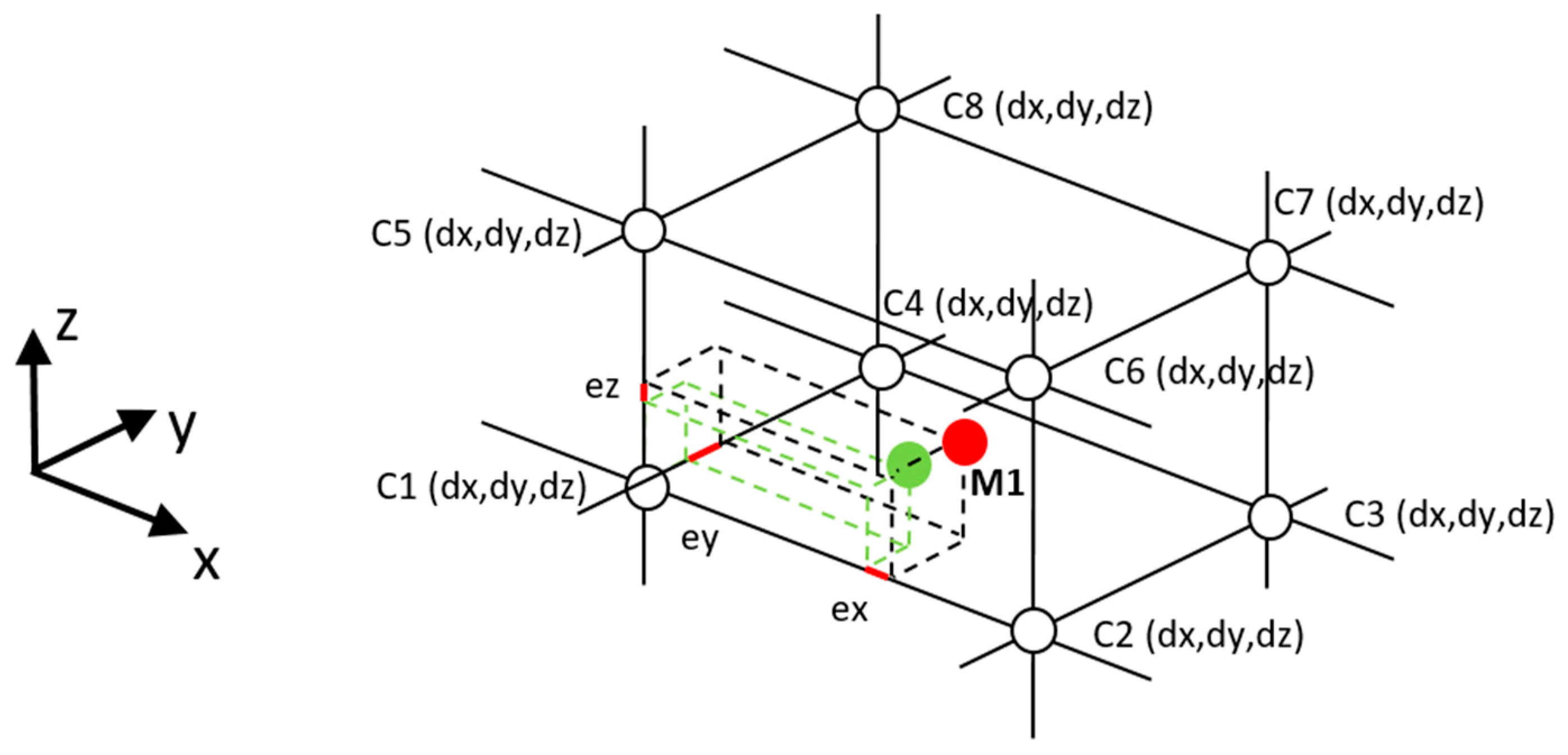
Correction data are calculated in the form of a structured three-dimensional mesh, where in each node the correction vector [dx, dy, dz] is defined, see Figure 1.

The basic task represents the calculation of the correction mesh, where the interpolation of correction values at the nodes compensate the evaluated error vector at the measured points. The correction value at any point in the workspace is calculated by trilinear interpolation [21] from the correction values at the nodes

$${\mathit{c}}_{\mathit{M}\mathbf{1}}=f\left(x_{M1},y_{M1},z_{M1},C1\left(dx,dy,dz\right),\dots , C8\left(dx,dy,dz\right)\right).$$

(3)

The algorithm in the proposed method decomposes deviations to main axes directions, and correction data are calculated for the main axes separately. The solution of the spatial problem is thus transformed from a three-dimensional problem to a 3 × 1-dimensional problem for the main machine tool axes X, Y, Z.

Figure 2 shows a one-dimensional scheme in which real workpiece geometry is measured at five measured points in the Y-axis direction and the compensation data are calculated only in the Y-axis direction. The correction mesh consists of nodes where the compensation value is calculated and the edges connect two adjacent nodes. These edges are not part of the correction data, but are important for calculating node displacements.

The measured point-correction value depends right on the cell where the point is located. For node displacement calculations from a measured point error, it is possible to select a more general procedure where the measured point also affects the further cells. The influence of the further cells may be important for cases with a significantly uneven distribution of measured points, and it acts as a filtering mechanism of the missing measured points.

2.1. Correction Mesh Design

The size of the mesh and the number of nodes in the main axis direction are the basic parameters for calculating the displacement of the nodes. These parameters are user-specified or calculated automatically. In case of an automatic approach, the mesh size is designed to include all measured points, and the number of cells is chosen equal to the number of measured points. A significantly higher number of nodes than measured points is inefficient in terms of the formation of mesh zones, where nodes are not sufficiently affected by the measured points. On the other hand, a significantly lower number of nodes cannot sufficiently ascertain the details of the measured shape.

The proposed method also works with an uneven distribution of measured points. Based on an equidistant distribution of nodes, it smooths zones with lower measured points density and determines the number of cells from the number of measured points, which appears satisfactory. In case of complex shapes or measured point distribution, it may be advantageous to design the mesh manually with full parameter controls.

An uneven distribution of measured points may lead to a situation with more than one measured point in a single cell. This state is not a problem for node displacement calculation because it is solved by an iterative procedure. Considering that each internal node affects eight cells of the mesh, it is not possible to calculate node displacement in each cell separately. The interpolation of displacement from eight nodes of one cell must correspond to the error value of the measured point in this cell. However, at the same time, the correction at each node must correspond to the remaining seven cells and the measured points located there.

The mesh can be designed both with an arbitrary edge length in the X, Y and Z directions and a distinct number of equidistantly distributed nodes in each direction. To create a three-dimensional mesh, the lowest number of nodes in each single direction is two. The proposed method is also applicable to one- and two-dimensional solutions, where the corrections in the second and third dimension have the same values and are only shifted positions of the nodes in the second and third dimension, respectively.

2.2. Equations of Node Displacements

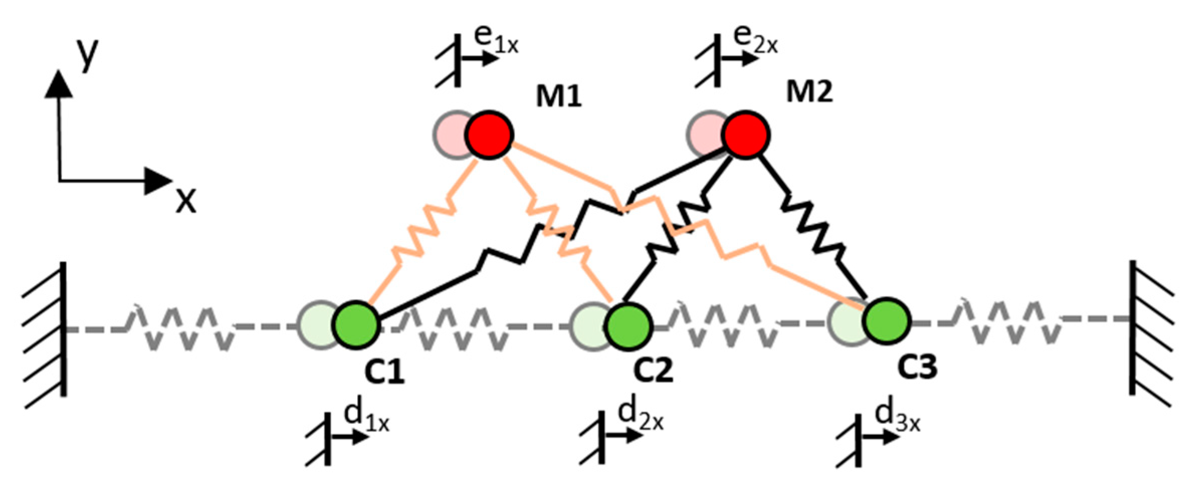
The calculation of node displacements is based on their connection with measured points. The connection is realized with imaginary springs, which connect the measured points with the nodes of the correction mesh. The measured point does not have to be connected only to the nodes of the cell in which it is located, but it can also be connected to the nodes of other cells. The displacement of the nodes is based on the fictitious force balance of the correction mesh, which deviates from the equilibrium state by the evaluated deviations at the measured points. Figure 3 shows a scheme for calculating the displacement of nodes in one row and direction, where the measured points also connect to nodes in further cells.

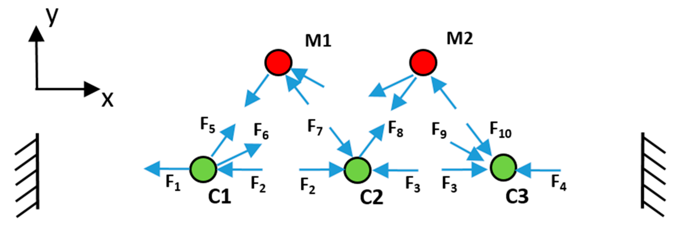
The input to the calculation is the initial distribution of nodes (C) and measured points (M) and the evaluated deviation at the measured point (e), and the output is the required displacement of the nodes (d). The product of the spring stiffness and the displacement of measured points produce the imaginary forces acting on the nodes. The imaginary springs connect the adjacent nodes, too, and the resulting force interaction scheme is shown in Figure 4.

To maintain the force balance according to Figure 4, $\sum {\mathit{F}}_i=0$ must apply for each node. The following system of equations can be derived for the displacement d_1x, d_2x and d_3x of nodes C1, C2 and C3, respectively:

$$\left[\begin{array}{ccc}2k+{\displaystyle {\displaystyle \sum }_{i=1}^3}{k}_{i1}& -k& 0\\ -k& 2k+{\displaystyle {\displaystyle \sum }_{i=1}^3}{k}_{i2}& -k\\ 0& -k& 2k+{\displaystyle {\displaystyle \sum }_{i=1}^3}{k}_{n1}\end{array}\right] \left[\begin{array}{c}{d}_{1x}\\ d_{2x}\\ d_{3x}\end{array}\right]=\left[\begin{array}{c}{\displaystyle {\displaystyle \sum }_{i=1}^2}{k}_{11}{p}_{i1}\\ \begin{array}{c}{\displaystyle {\displaystyle \sum }_{i=1}^2}{k}_{21}{p}_{21}\\ {\displaystyle {\displaystyle \sum }_{i=1}^2}{k}_{31}{p}_{n1}\end{array}\end{array}\right],$$

(4)

where k [N·m⁻¹] is the stiffness of the springs between nodes of the mesh, k_ij [N·m⁻¹] is the stiffness between the i-th measured point and the j-th node and p_ij = e_i − d_j is the variation of the distance between the i-th measured point and j-th node in the direction investigated. The resulting system of equations consists of a three-diagonal matrix, which is effective in calculating the inverse matrix for a system of equations solution. Generally, for N measured points acting on M nodes, the j-th equation of the system of equations is derived in the form

$$\left[\begin{array}{ccc}-k& 2k+{\displaystyle {\displaystyle \sum }_{i=1}^M}{k}_{i2}& \begin{array}{c}-k\end{array}\end{array}\right].\left[\begin{array}{c}{d}_{j-1}\\ d_j\\ \begin{array}{c}{d}_{j+1}\end{array}\end{array}\right]=\left[\begin{array}{c}\begin{array}{c}{\displaystyle {\displaystyle \sum }_{i=1}^N}{k}_{ji}{p}_{ji}\end{array}\end{array}\right].$$

(5)

The key feature of the proposed connection is the constant stiffness of springs connecting the nodes and the variable stiffness of the springs connecting the measured points to nodes:

$$k_{ij}=\frac{l_e}{l_{ij}}k,$$

(6)

where l_e [m] is the length of the cell edge in the calculated direction and l_ij [m] is the distance from the measured point to the connected node in the calculated direction. If the measuring point was identical with the mesh node, the connection stiffness would be infinite. In the proposed algorithm, this case is treated so that the displacement of the node is equal to the evaluated deviation of the measured point. The connection stiffness between the measured point and the given node is not considered.

2.3. Calculation of Node Displacements

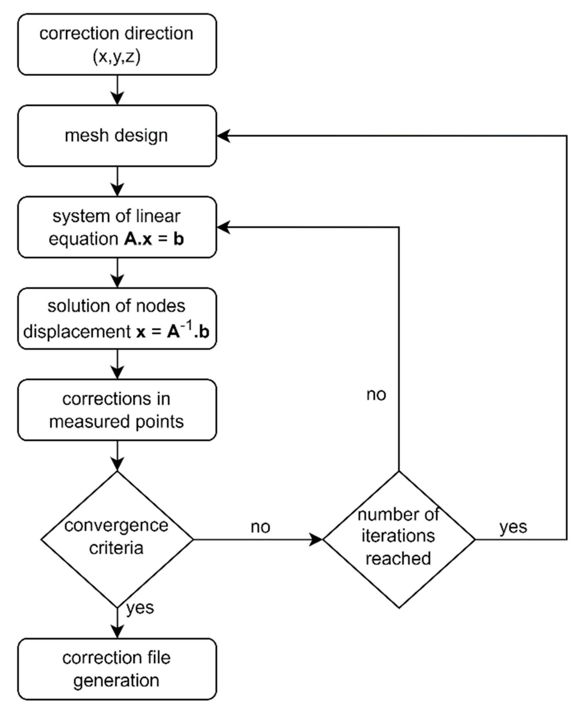
For each direction X, Y, Z, the displacement of the correction mesh nodes is solved separately. A set of linear Equation (5) is compiled for the node displacement calculations in the selected direction. The correction in the measured points calculated by interpolation from the nodes is not equal to the evaluated error at the measured points after this calculation. This difference is based on the connection of the measured points and nodes by flexible springs, except in the case when the measured point is identical with any node. By connecting the springs, the nodes always move less than the specified offset of the measured point. To increase accuracy, the proposed method includes an iterative algorithm; see Figure 5. A correction mesh with a defined dimension and a number of nodes is set up for the selected direction. From the knowledge of the position of the nodes and the measured points, the equation for the displacement of the node points (5) is compiled and calculated. The correction of the measured point is then calculated by interpolation from the calculated displacement. The difference between the evaluated and the required correction is added to the evaluated correction in the following iterative calculation.

The end of the iteration calculation is given by reaching the maximum number of iterations, or by achieving the required accuracy. The iterative calculation can also be terminated by reaching the maximum defined node displacements. If the maximum number of iterations is reached, but the required accuracy is not reached and the calculation no longer converges, it is necessary to adjust the mesh. The reason may be, for example, several measured points with different required corrections in one cell. After the successful calculation of the node displacements, a file with correction data is compiled containing the mesh dimensions, the number of nodes in individual directions and the displacement values at the nodes.

3. Results

The proposed method was tested by simulation and subsequently on a real control system in quasi-stationary positioning without machining, where the current correction value in the control system was checked. Finally, the test workpiece was machined to compare the achieved accuracy with corrections both on and off.

3.1. Numeric Simulation

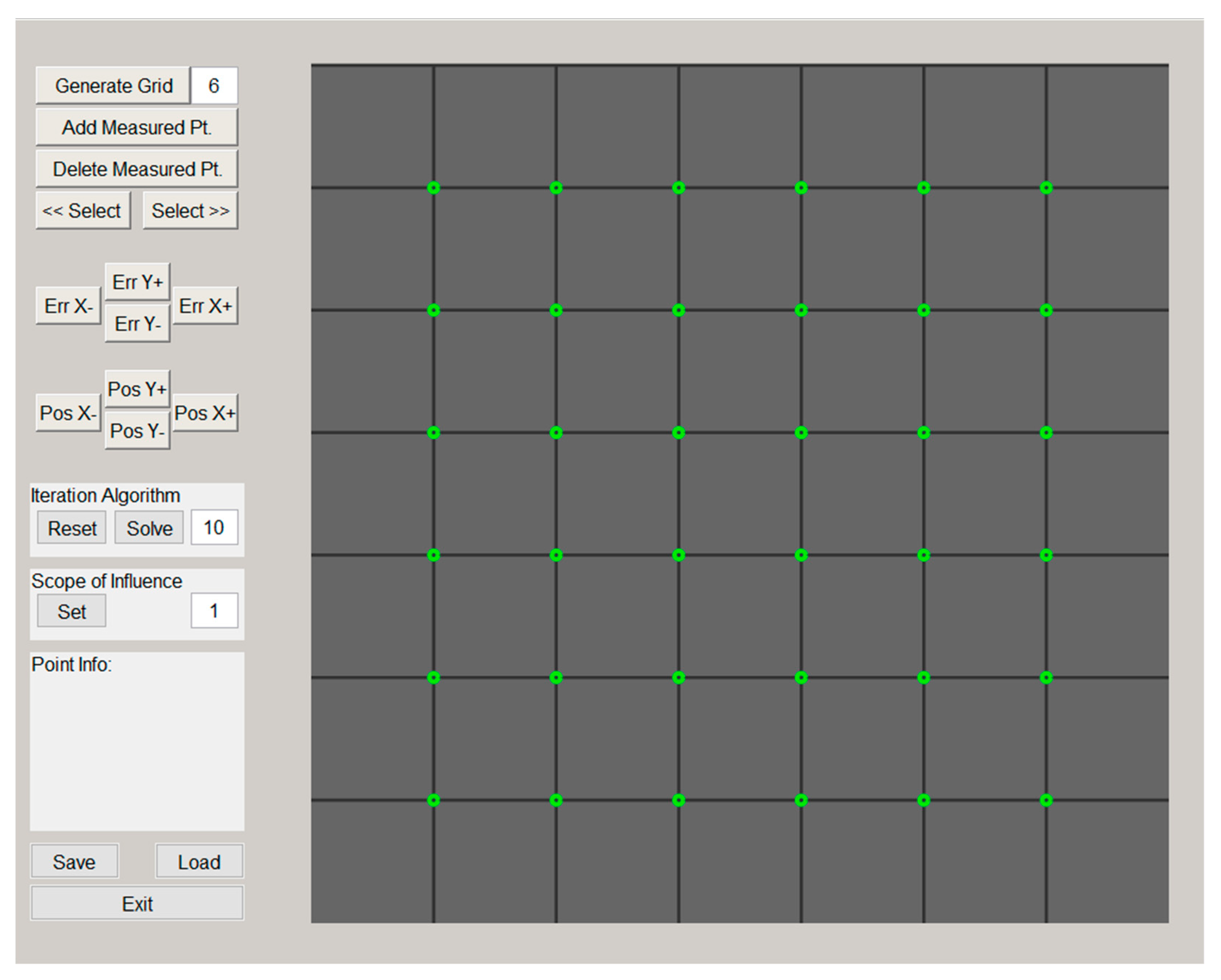
To verify the proposed method, an application was created in the Matlab environment (Figure 6), which calculates the correction mesh based on the entered deviations at selected points. Output of the application is a calculated correction mesh and summary information about the achieved accuracy, i.e., the difference between the requested and the calculated corrections.

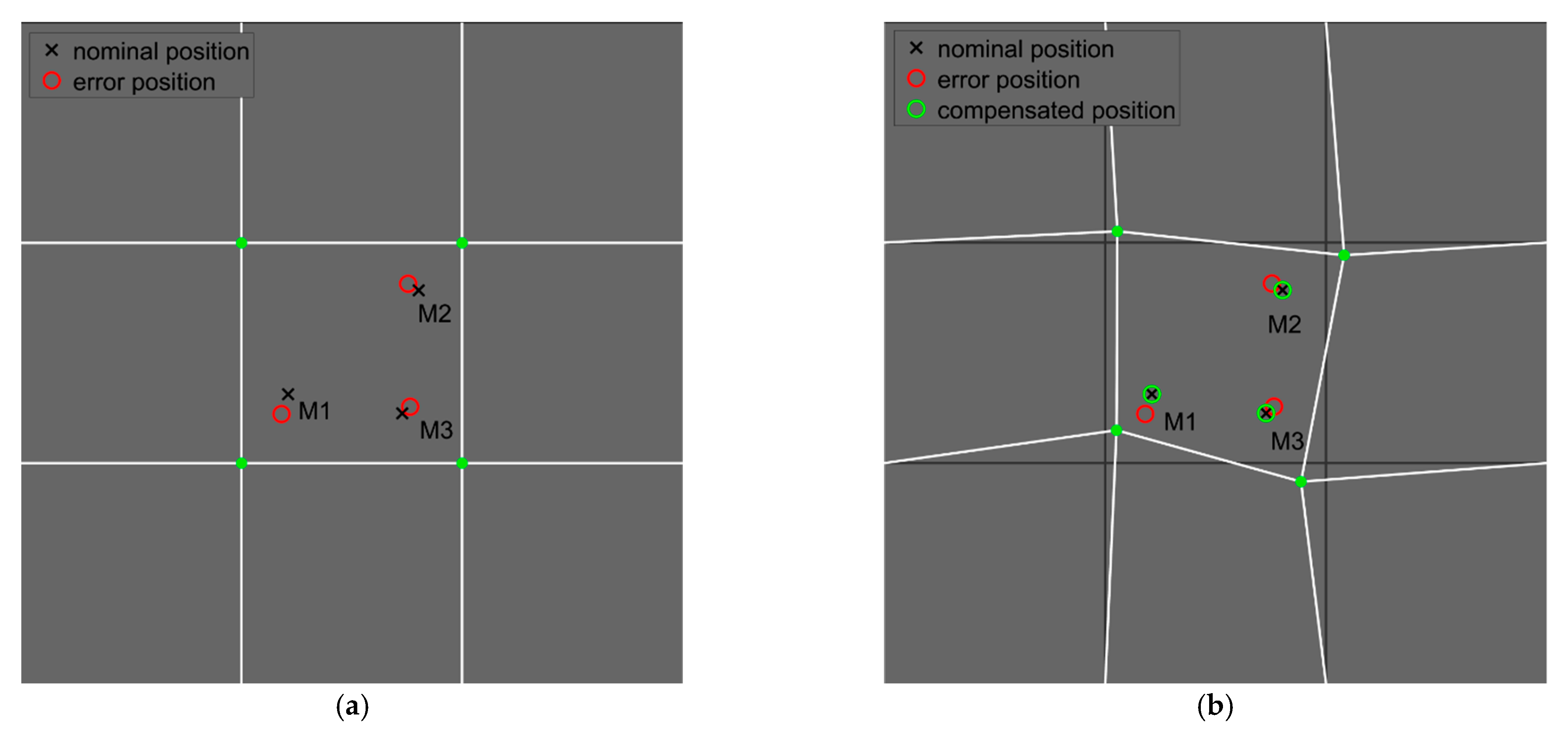
A correction square mesh with 3 × 3 cells was generated for testing, where zero corrections in the X, Y directions were considered at the outer boundary of the mesh; see Figure 7a.

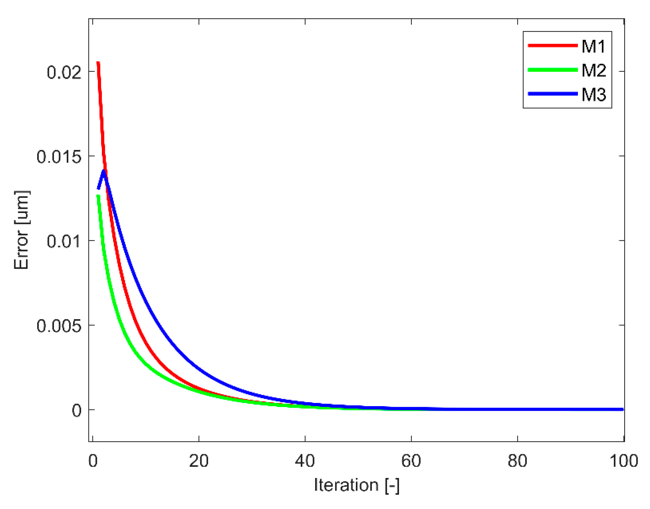
Three measured points with position deviations were positioned in the middle cell. To test the robustness of the proposed method, a deviation was defined with a different direction at each point: ${\mathbf{\epsilon }}_{M1}=\left[0.10, 0.30\right] \mathrm{mm}, {\mathbf{\epsilon }}_{M2}=\left[0.16,-0.10\right] \mathrm{mm}, {\mathbf{\epsilon }}_{M3}=\left[-0.12,-0.10\right] \mathrm{mm}.$ The calculated correction mesh after 100 iterations is shown in the Figure 7b, where the deviations are 100× magnified. Convergence of the difference between the nominal and reconstructed positions of the measured points is presented in Figure 8. Although three measured points in one cell had prescribed nearly opposite position deviations, the position was reconstructed with an accuracy of more than 99.98% for all points.

3.2. Verification on Machine Tool without Machining

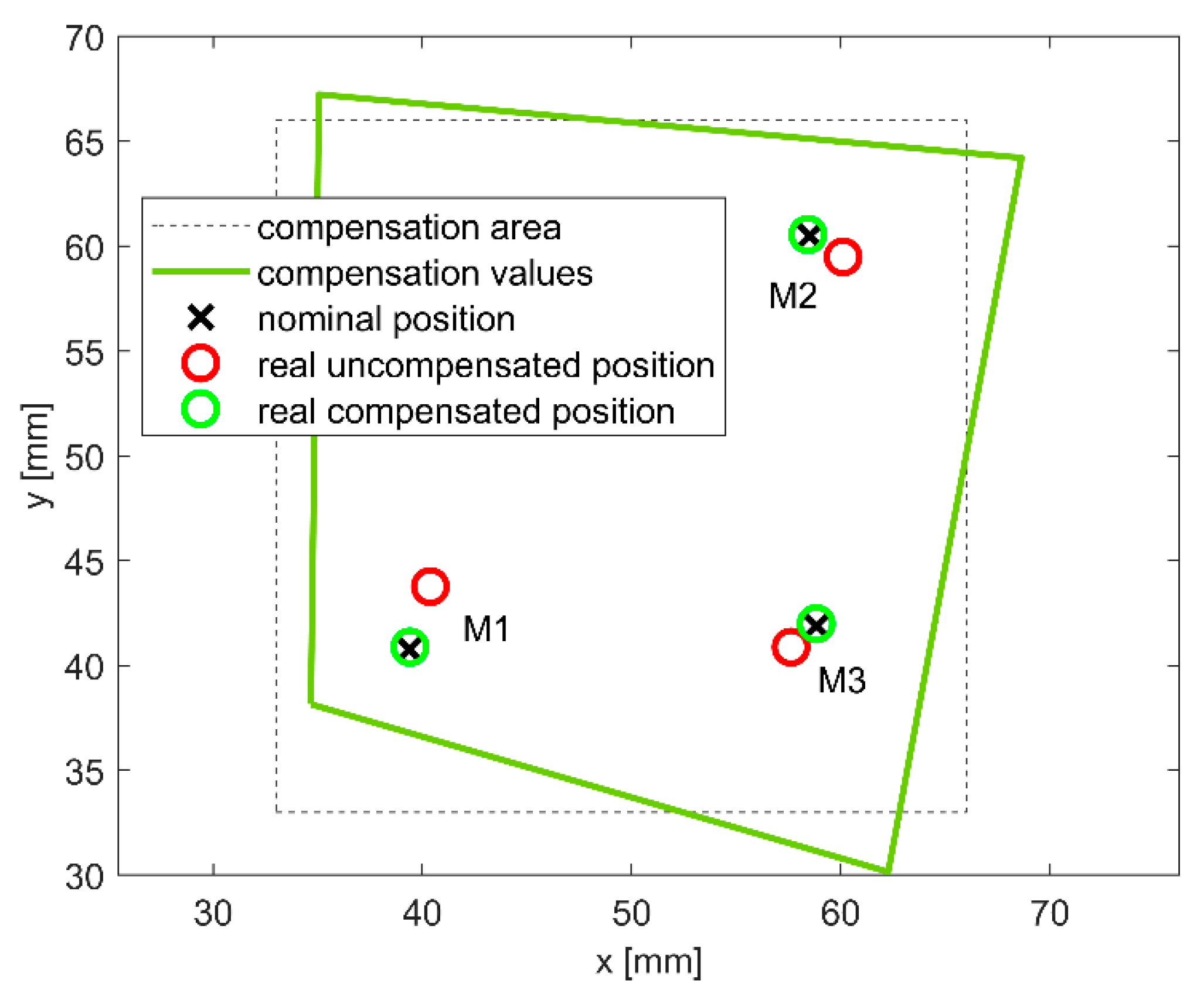
After successful verification of the correction mesh calculation within the simulation, the proposed algorithm was tested on a Siemens Sinumerik 840D sl control system in quasi-stationary positioning. A Cycle 996 VCS Rotary is activated in this control system, where VCS denotes Volumetric Compensation System. As of version 3.0 of Cycle 996, up to three axes may be used for compensation, where the compensation value is calculated from the actual machine tool position and compensation data. The compensation data is entered in the form of an *.spf file, where following the initialization header, the compensation values are in the form

$$\mathrm{E}996\_\mathrm{GP}\left(\mathrm{gp}1, \mathrm{gp}2, \mathrm{gp}3, \mathrm{compval}1, \mathrm{compval}2, \mathrm{compval}3\right),$$

where gp1, gp2 and gp3 denote a position in the three-dimensional grid of input axes and compval1, compval2 and compval3 the deviations in that position for output axes. An example of the *.spf file is in the Appendix A, where the file structure is explained in detail. In accordance with the proposed method, the compensation data in each axis may be defined with a different number of nodes. The principle of calculating the correction value is based on interpolation in a three-dimensional mesh of compensation values that is integrated directly into a real-time core. However, detailed information about this calculation is not available in the documentation. Therefore, in accordance with the numerical simulation, a correction mesh with 3 × 3 cells was chosen, where the three selected test points lay in the middle cell of this network. At these points, a deviation from the desired position in the directions of the X, Y axes was prescribed ${\epsilon }_{M1}=\left[0.10, 0.30\right] \mathrm{mm}, {\epsilon }_{M2}=\left[0.16,-0.10\right] \mathrm{mm}, {\epsilon }_{M3}=\left[-0.12,-0.10\right] \mathrm{mm}$ for points M1, M2 and M3, respectively. These deviations and nominal positions were used to calculate the correction network and for compilation of the *.spf file for the control system. Next, the machine tool was positioned to the measured points, where the current compensation value was read from the control system. The results are shown in Figure 9, where the deviations are magnified 100× for clarity, and it is clear that there was a significant reduction in positional deviation. Specifically, the positional deviation was reduced by 96%, 92% and 94% for points 1, 2 and 3, respectively. These results show that the control system calculates the correction correctly. Refinement of the correction mesh to place each measuring point in a separate cell will produce even better results. However, in the selected case, the compensation error was already 1.2 μm, 1.1 μm and 1.2 μm for points M1, M2 and M3, respectively. All these values are considerably superior to the achievable accuracy of the selected machine tool.

3.3. Verification on Machine Tool with Machining

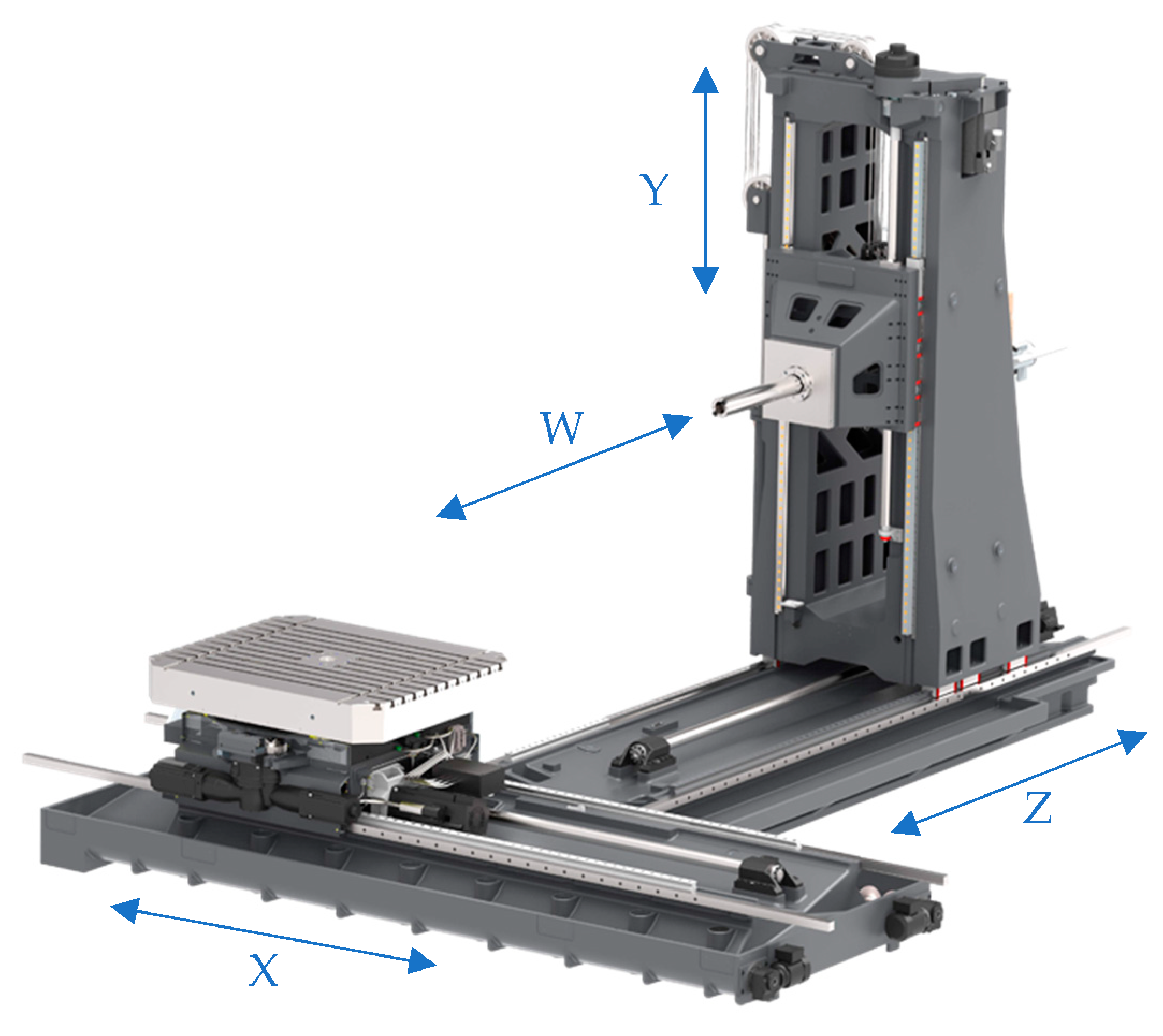
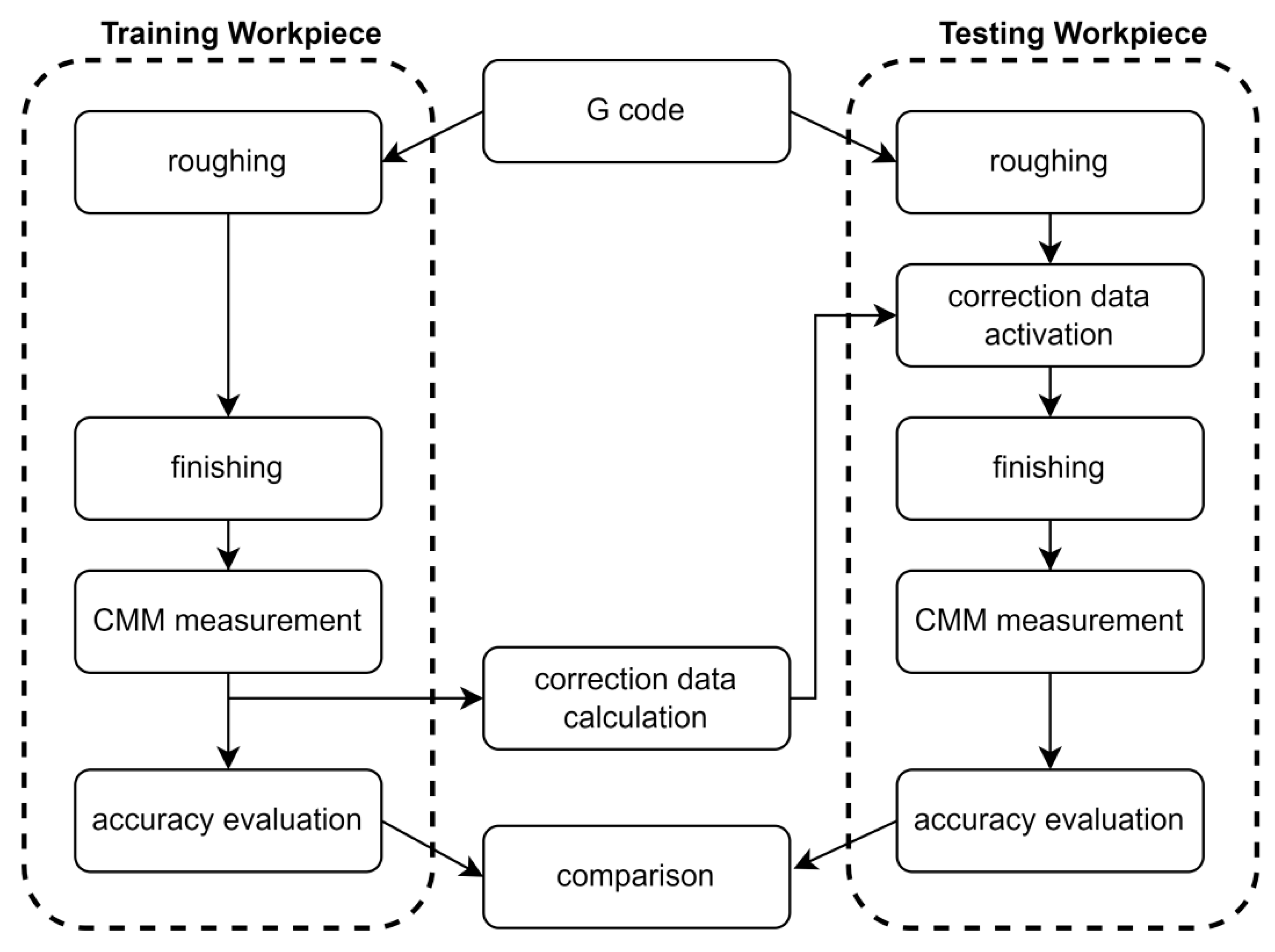
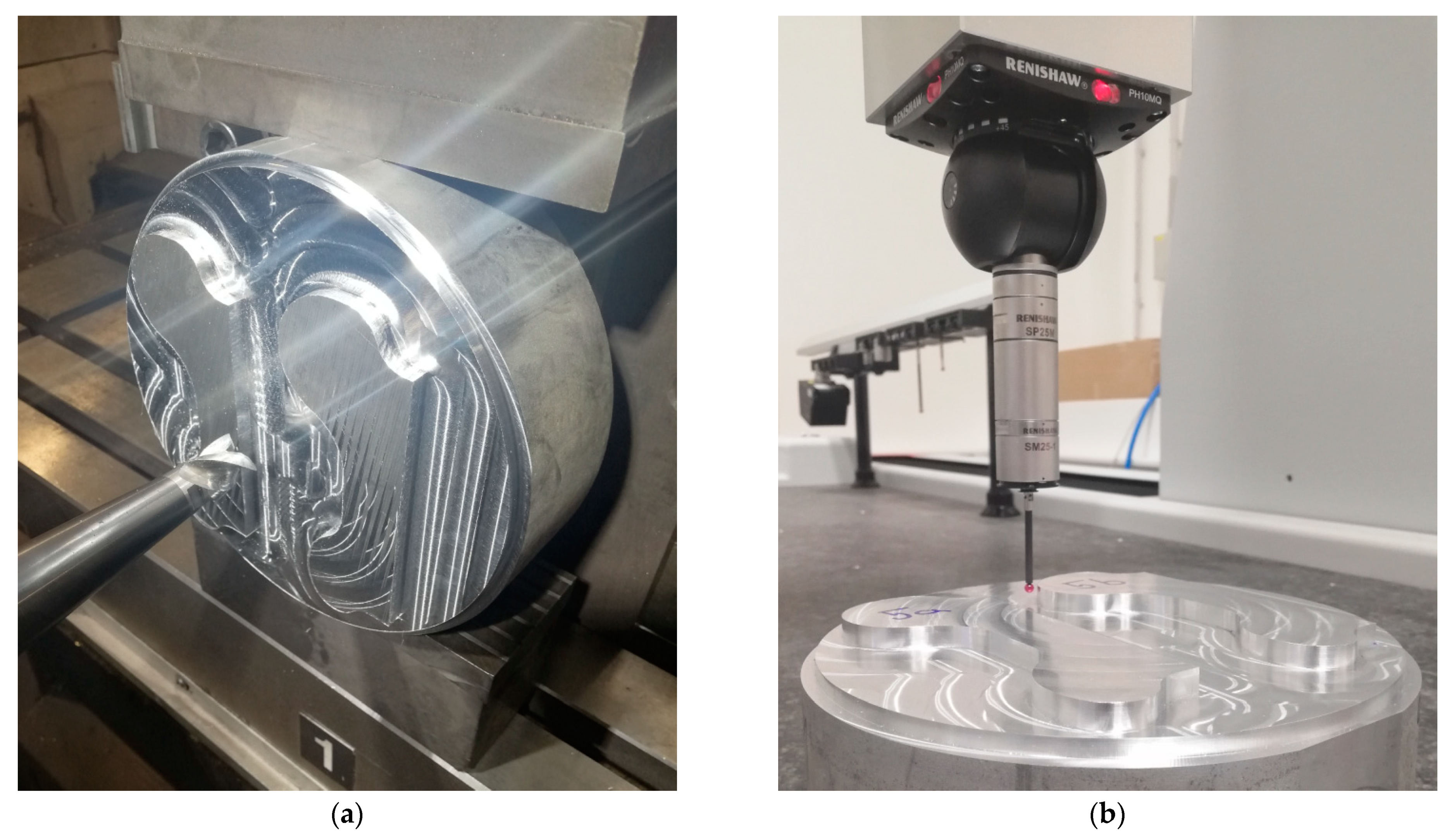
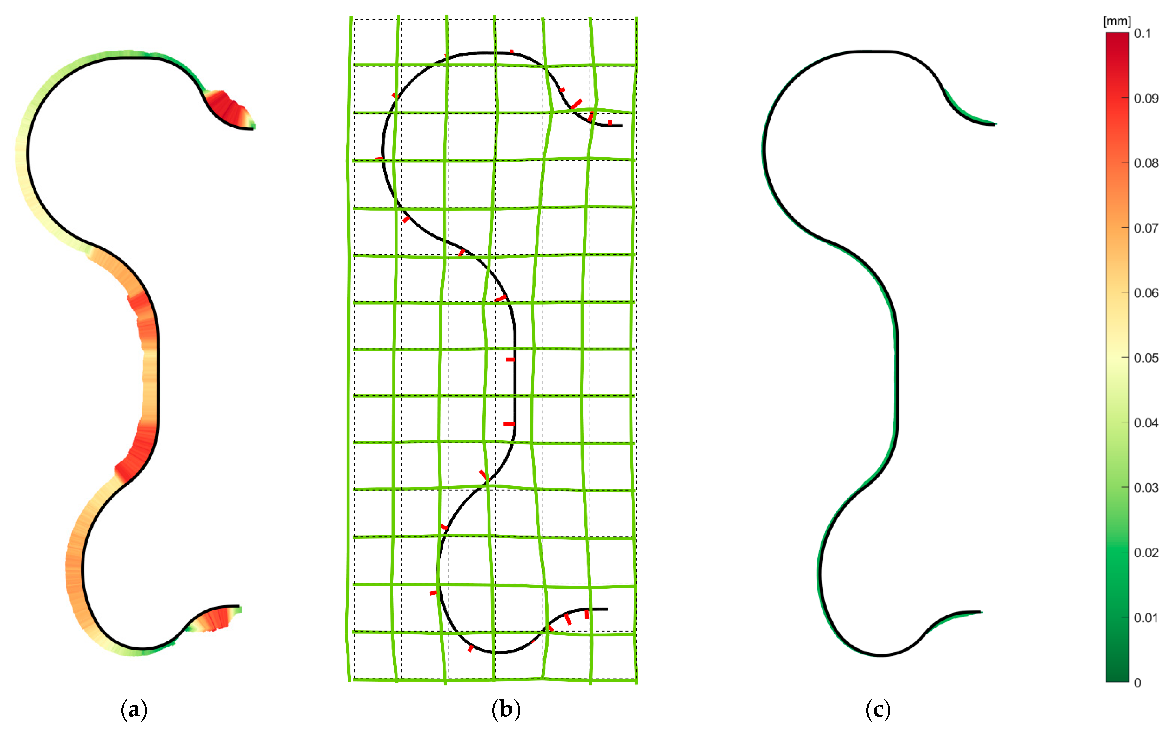
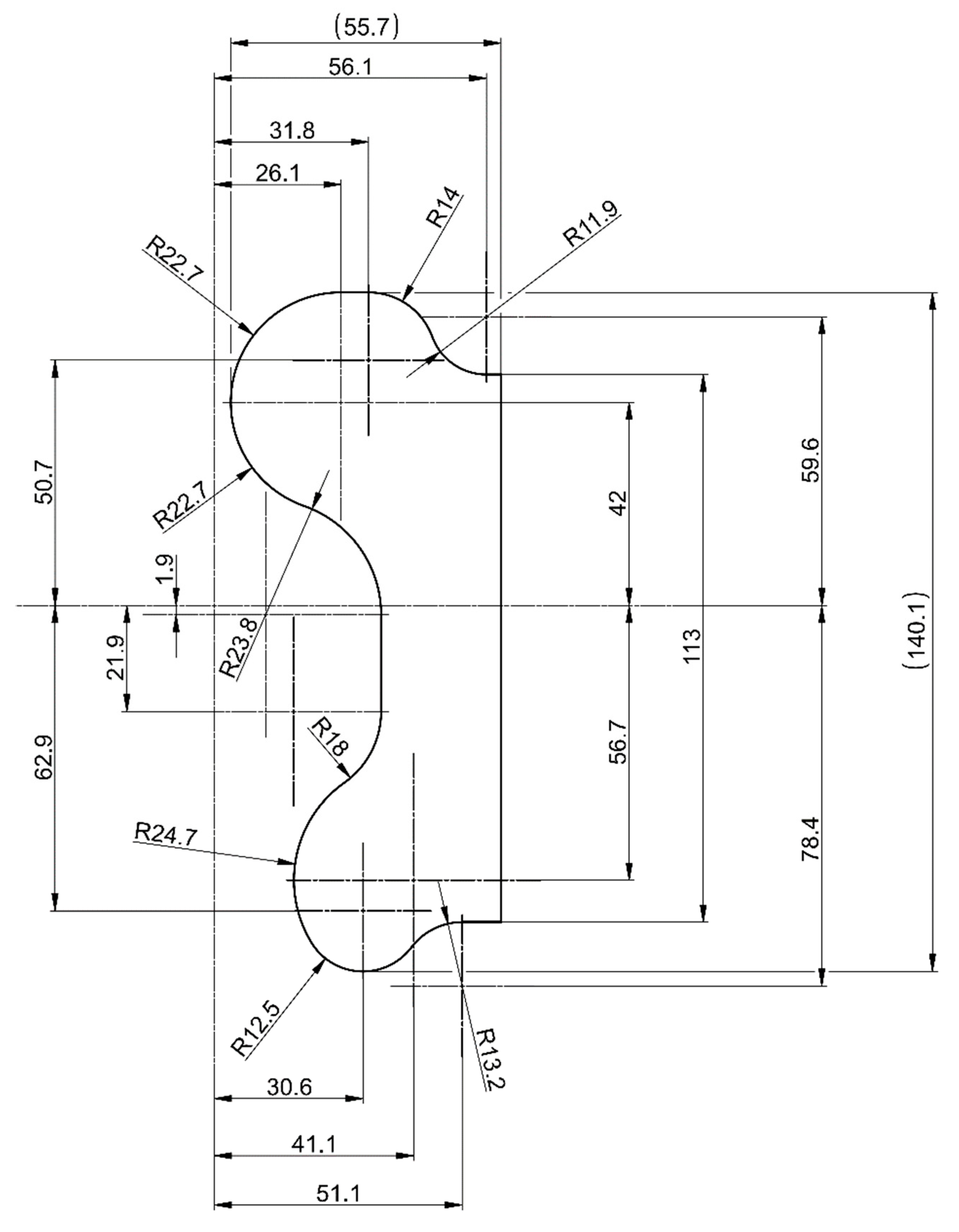
A machining test was performed on a three-axis machining center to verify the proposed method on a real part, and it is shown in Figure 10. Aluminum material AL7075 was chosen, and the tool used for machining was D20 mm solid carbide head with three flutes with 40° different helixes for aluminum machining. The tool was mounted in a hydraulic expansion tool holder with the interface ISO SK 50. The geometry of the designed part consists of linear and circular sections, and its technical drawing is provided in Appendix B. The NC program was developed in CAM software Siemens NX 12. A flow chart of the experiment is shown in Figure 11 and consists of two parts: the training and testing phases. The aim of the training phase was to evaluate the accuracy of machining without the proposed method and to calculate the correction data. An identical tool was used for roughing and finishing, where the cutting conditions are given in

Table 1. Cutting conditions for workpiece machining.

Parameter	Roughing	Finishing
Feed rate	1500 mm/min	750 mm/min
Spindle speed	5000 rpm	5000 rpm
Feed per tooth	0.1 mm/tooth	0.05 mm/tooth

, and they were set with accordance to the tool manufacturer’s recommendation. To increase the surface quality, Cycle 832—High Speed Settings was activated in the control system in the form CYCLE832(0.03, FINISH,1), i.e., tolerance of 0.03 mm was prescribed for finishing for a program without orientation of the tool. After the final machining, the training piece was measured on a Coord3 coordinate measuring machine with a Renishaw SP25M scanning probe; see Figure 12. The deviation of the real geometry from the required one is plotted in Figure 13a, and it reached 0.098 mm.

3.3.1. Correction Data Calculation

The Renishaw SP25M scanning probe measured 2480 points along the shape. Measuring with a scanning probe is a privilege of high-tech CMM, while touch-trigger probes are standard tools for CMM. Alternatively, if the measurement was performed directly on a machine tool, scanning-probe utilization would also be difficult. Therefore, only 21 points were selected manually to calculate the correction mesh. These points are located with respect to contour error distribution, where in the zones with higher deviations, more points were selected. Especially in the smallest inner radii, the errors reached the maximum and denser discretization was used there. The distance from each measured point to the nearest other one was calculated, and the mean value of these distances defined the mesh density. The resulting mesh has 6 × 14 × 1 cells in the directions of the X, Y and Z axes and is shown in the graph in Figure 13b, in which the selected measured points are also shown. The calculation of the correction mesh converged rapidly, and 96 iterations were enough to reduce the deviation by more than 98%. The total time of calculation in Matlab was less than 10 s, but it is worth stating that the algorithm is ready for optimization. The correction mesh must be defined in the global machine coordinate system, even if coordinate system transformation is activated for machining.

3.3.2. Testing Workpiece Machining

The testing workpiece was machined using the identical NC programs, as in the case of the training workpiece, and all technological conditions remained the same as well. The workpiece was fixed in the machine vice so that the testing position was identical to the training one. Roughing was performed without correction data activation, because an allowance (0.5 mm) significantly exceeds maximal geometric deviations (0.098 mm), and the correction data were activated for finishing only. After finishing, the testing workpiece was measured using a CMM with a scanning probe, and the deviations were evaluated. The results are shown in Figure 13c, and it is evident that there was a significant reduction in deviation. The maximum value reached 14 μm and successfully verified the proposed method.

4. Discussion

A numerical simulation verified the proposed method with very good results, where the position deviation of the simulated points was almost suppressed, even if three points were located in one cell of the correction mesh. Using the same points and the same correction mesh within the real Sinumerik 840D sl control system also achieved very promising results. Nevertheless, the reduction in the position deviation was a little weaker. In that case, the correction calculation was run fully under the control system, and it is not possible to comprehend the algorithm. The machining test on a three-axis machining center consisted of training and testing workpieces, where the training workpiece was machined with a maximal geometric deviation of 98 µm. This value is slightly above the expected one, but it corresponds to the actual state of the machine tool and other conditions. Based on the calculated correction mesh, the deviation of 98 µm was reduced to 14 µm, where all parameters and settings remained constant. The only single difference was the length of time needed to perform the evaluation, where measuring on a CMM, calculating the correction mesh and fixturing of the testing workpiece took about 90 min. During this time, the machine tool did not machine and the ambient temperature remained constant. The thermoelastic effects need not be considered; however, no machine temperatures were recorded within the experiment. Based on trace records, the machine tool position repeatability is significantly below 1 µm and the actual feed rate was nearly identical to the set value. The non-uniform results of achieved accuracy might come from various tool-engagement angles, where the different tool radial loading resulted in tool deflection. The largest deflections were always identified in the smallest inner radii, which are just slightly larger than the tool-used radius. Both chatter and vibrations were not registered during machining. The setting of the calculation consists of the area of space discretization, the area of influence of the measured points and the maximum number of iterations. All presented results are considered to be very promising, and machining using a more precise machine tool would probably lead to even better results.

The main advantage of the method represents compensation of all shape-error contributions, i.e., the positioning error of the machine tool, compliance of the machine tool and the workpiece, errors in the control system or NC program, etc. If more identical workpieces are machined, it is only necessary to measure the first one, since the compensation data remain constant for the following workpieces. This assumption takes into account the constant accuracy of the machine and the constant position of the parts in the working space of the machine tool. It neglects the effect of tool wear and does not respect changes in machine tool geometry caused by thermal loads. A great benefit of the proposed method is the increase in machining accuracy without modification of the NC code, since modifying that code is not a trivial task.

The main drawback is the principle of the method itself, where a training workpiece needs to be finished to determine the corrections. If the real shape of the training workpiece is larger than the nominal shape, corrective machining of the training workpiece is possible. On the other hand, if there are zones with shape undercutting below geometric tolerances, the workpiece cannot be corrected anymore. This procedure can be eliminated by semi-finishing when the final shape is machined with sufficient allowance to avoid undercutting. The workpiece would be measured after the semi-finishing, and the compensation data would then be calculated for the final machining.

This method does not generally increase the accuracy of the machine tool, but it only adapts tool trajectory for a given workpiece. Theoretically, machine compensation data in the same position may be different for a different workpiece. The approach presented does not replace the static volumetric compensations of machine tools, but it allows for an increase in the geometric accuracy of the machined workpiece.

Follow-up research will be focused on two areas. The first is an extension of the method for control systems that do not allow directly writing to volumetric correction tables, or have volumetric corrections based only on the kinematic model error principle, where arbitrary compensation within the whole workspace is not feasible. One of the possible solutions is writing the correction values in the form of temperature compensations. The use of an external industrial computer (IPC), such as an EDGE device communicating with the machine control system, is considered. In such a configuration, the correction values will be calculated in the IPC based on the current machine position and sent to the machine control system online. In this solution, the corrections may be affected by the time delay caused by non-real-time communication between the IPC and the control system. The second area of research is in-process on-machine measurement, which would eliminate the transport of the workpiece to the CMM, back to the machine tool and its setting in the working space. Especially for large and heavy workpieces, this type of manipulation is challenging and time consuming. This approach would significantly shorten the entire measurement process. The big challenge is to increase the accuracy of the machine tool in the measuring mode when additional devices are considered to compensate for its inaccuracy. At the same time, it would be advantageous to implement standard metrology software in the machine tool control system in order to provide the same functionality as the CMM.

5. Conclusions

This article describes a method for increasing the geometric accuracy of a machined workpiece. The method is based on the ad hoc determination of machine tool compensation data from the difference between the nominal and real workpiece geometries. The method was successfully verified by simulation and machining a part, where the geometric accuracy of the workpiece was increased by more than 85% during machining. Summary points can be defined as:

• The method extends correction data from several measured points to overall workpiece shape;
• This extension is based on spring-connected nodes and measured points, where deflections come from external metrology;
• The method works for paired machinetool-workpiece in a given position only, any changes in workpiece position or design yield to new correction data evaluation;
• Direct implementation in Siemens Sinumerik 840D sl control system;
• The method does not eliminate all sources of workpiece geometric error.
• This method is time consuming in terms of evaluating geometric deviations, but for machining high-precision parts it represents one of the ways to achieve the highest accuracy.

References

1. Okafor, A.C.; Ertekin, Y.M. Derivation of machine tool error models and error compensation procedure for three axes vertical machining center using rigid body kinematics. Int. J. Mach. Tools Manuf. 2000, 40, 1199–1213. [Google Scholar] [CrossRef]
2. Holub, M.; Jankovych, R.; Vetiska, J.; Sramek, J.; Blecha, P.; Smolik, J.; Heinrich, P. Experimental Study of the volumetric error effect on the resulting working accuracy—Roundness. Appl. Sci. 2020, 10, 6233. [Google Scholar] [CrossRef]
3. Schwenke, H.; Knapp, W.; Haitjema, H.; Weckenmann, A.; Schmitt, R.; Delbressine, F. Geometric error measurement and compensation of machines—An update. CIRP Ann. 2008, 57, 660–675. [Google Scholar] [CrossRef]
4. Ramesh, R.; Mannan, M.A.; Poo, A.N. Error compensation in machine tools—A review. Int. J. Mach. Tools Manuf. 2000, 40, 1235–1256. [Google Scholar] [CrossRef]
5. Groos, L.; Held, C.; Keller, F.; Wendt, K.; Franke, M.; Gerwien, N. Mapping and compensation of geometric errors of a machine tool at different constant ambient temperatures. Precis. Eng. 2020, 63, 10–17. [Google Scholar] [CrossRef]
6. Mareš, M.; Horejš, O.; Havlík, L. Thermal Error compensation of a 5-axis machine tool using indigenous temperature sensors and CNC integrated python code validated with a machined test piece. Precis. Eng. 2020, 66, 21–30. [Google Scholar] [CrossRef]
7. Mian, N.S.; Fletcher, S.; Longstaff, A.P.; Myers, A. Efficient estimation by FEA of machine tool distortion due to environmental temperature perturbations. Precis. Eng. 2013, 37, 372–379. [Google Scholar] [CrossRef] [Green Version]
8. Bringmann, B.; Küng, A.; Knapp, W. A Measuring artefact for true 3D machine testing and calibration. CIRP Ann. 2005, 54, 471–474. [Google Scholar] [CrossRef]
9. Li, C.; Liu, X.; Li, R.; Wu, S.; Song, H. Geometric error identification and analysis of rotary axes on five-axis machine tool based on precision balls. Appl. Sci. 2019, 10, 100. [Google Scholar] [CrossRef] [Green Version]
10. Ibaraki, S.; Kudo, T.; Yano, T.; Takatsuji, T.; Osawa, S.; Sato, O. Estimation of three-dimensional volumetric errors of machining centers by a tracking interferometer. Precis. Eng. 2015, 39, 179–186. [Google Scholar] [CrossRef] [Green Version]
11. ISO 10791-7: 2020; Test Conditions for Machining Centres—Part 7: Accuracy of Finished Test Pieces. ISO: Geneva, Switzerland, 2020.
12. Xiang, S.; Altintas, Y. Modeling and compensation of volumetric errors for five-axis machine tools. Int. J. Mach. Tools Manuf. 2016, 101, 65–78. [Google Scholar] [CrossRef]
13. Choi, J.P.; Min, B.K.; Lee, S.J. Reduction of machining errors of a three-axis machine tool by on-machine measurement and error compensation system. J. Mater. Processing Technol. 2004, 155–156, 2056–2064. [Google Scholar] [CrossRef]
14. Gao, W.; Haitjema, H.; Fang, F.Z.; Leach, R.K.; Cheung, C.F.; Savio, E.; Linares, J.M. On-machine and in-process surface metrology for precision manufacturing. CIRP Ann. 2019, 68, 843–866. [Google Scholar] [CrossRef] [Green Version]
15. Wu, B.; Yin, Y.; Zhang, Y.; Luo, M. A new approach to geometric error modeling and compensation for a three-axis machine tool. Int. J. Adv. Manuf. Technol. 2019, 102, 1249–1256. [Google Scholar] [CrossRef]
16. Fu, G.; Fu, J.; Shen, H.; Yao, X.; Chen, Z. NC codes optimization for geometric error compensation of five-axis machine tools with one novel mathematical model. Int. J. Adv. Manuf. Technol. 2015, 80, 1879–1894. [Google Scholar] [CrossRef]
17. Wang, Z.; Maropolous, P.G. Real-time error compensation of a three-axis machine tool using a laser tracker. Int. J. Adv. Manuf. Technol. 2013, 69, 919–933. [Google Scholar] [CrossRef]
18. Kuo, C.-H.; Chen, P.-C. On-Machine measurement and error compensation for 6061 aluminum alloy hexagonal punch using a turn-milling machine. Machines 2021, 9, 180. [Google Scholar] [CrossRef]
19. Ma, W.; He, G.; Han, J.; Xie, Q. Error compensation for machining of sculptured surface based on on-machine measurement and model reconstruction. Int. J. Adv. Manuf. Technol. 2020, 106, 3177–3187. [Google Scholar] [CrossRef]
20. Zhao, Z.; Xu, T. A novel approach for process shape construction in adaptive machining of curved thin-walled part. Precis. Eng. 2021, 67, 282–292. [Google Scholar] [CrossRef]
21. Vahebi Nojedeh, M.; Habibi, M.; Arezoo, B. Tool path accuracy enhancement through geometrical error compensation. Int. J. Mach. Tools Manuf. 2011, 51, 471–482. [Google Scholar] [CrossRef]
Figure 1. Measured point M1 surrounded by the correction mesh. The nominal and real positions of the measured point are marked in green and red, respectively.
Machines 10 00288 g001
Figure 2. Scheme of a 1-dimensional task for correction mesh calculation.
Machines 10 00288 g002
Figure 3. Scheme of a 1-dimensional task (x-direction) with 2 measured points (M1, M2) and 3 nodes (C1, C2, C3).
Machines 10 00288 g003
Figure 4. Elastic forces resulting from the measured points and node displacements.
Machines 10 00288 g004
Figure 5. Flow chart of node translation calculations.
Machines 10 00288 g005
Figure 6. Application for testing of the proposed method.
Machines 10 00288 g006
Figure 7. Numeric simulation of correction mesh calculation: (a) nominal position with an arbitrary error at every point; (b) compensated position evaluated from the correction mesh.
Machines 10 00288 g007
Figure 8. Difference between the nominal and compensated point positions depending on the number of iterations.
Machines 10 00288 g008
Figure 9. Nominal, real uncompensated and real compensated positions of measuring points in the Siemens Sinumerik 840D sl control system.
Machines 10 00288 g009
Figure 10. Machining center used for the proposed method verification.
Machines 10 00288 g010
Figure 11. Flow chart of training and testing workpiece machining.
Machines 10 00288 g011
Figure 12. Machining and measuring of the workpiece: (a) machining on a three-axis machining center; (b) measuring on CMM using a Renishaw SP25M scanning probe.
Machines 10 00288 g012
Figure 13. Increase in workpiece accuracy: (a) evaluation of training workpiece; (b) generation of correction mesh based on selected measured points; (c) evaluation of testing workpiece accuracy with an activated ad hoc correction table.
Machines 10 00288 g013