Abstract
Induction motors, the key equipment for rotating machinery, are prone to compound faults, such as a broken rotor bars and bearing defects. It is difficult to extract fault features and identify faults from a single signal because multiple fault features overlap and interfere with each other in a compound fault. Since current signals and vibration signals have different sensitivities to broken rotor and bearing faults, a multi-channel deep convolutional neural network (MC-DCNN) fault diagnosis model based on multi-source signals is proposed in this paper, which integrates the original signals of vibration and current of the motor. Dynamic attenuation learning rate and SELU activation function were used to improve the network hyperparameters of MC-DCNN. The dynamic attenuated learning rate can improve the stability of model training and avoid model collapse effectively. The SELU activation function can avoid the problems of gradient disappearance and gradient explosion during model iteration due to its function configuration, thereby avoiding the model falling into local optima. Experiments showed that the proposed model can effectively solve the problem of motor compound fault identification, and three comparative experiments verified that the improved method can improve the stability of model training and the accuracy of fault identification.
1. Introduction
As the key equipment for energy conversion in industrialization, induction motors are widely used in industrial production and daily life. Once a fault occurs, it will directly affect production efficiency and even cause casualties [1]. Broken rotor bars and motor bearing defects are two major motor faults with high frequencies [2]. With the increasing complexity of working conditions and the increasing working hours for machinery, the probability of multiple fault phases occurring together is also greatly increased [3].
In terms of motor mechanism and modeling, reference [4] points out that the occurrence and development of all faults in a motor have certain theoretical bases, and only by clarifying the mapping relationship between fault phenomena and mechanisms can the fault sources be accurately judged. For example, Jiang B et al. [5] analyzed the fault characteristics of stator winding by establishing the dynamic model of induction motor, and the proposed new scheme can effectively separate faults. Reference [6] deduces the mapping relationship between fault frequency and fault mechanism by establishing a motor simulation model. However, due to the influence of the harmonic of the power supply and the inevitable accompanying heat and external noise during the operation of the motor, the method based on mechanism analysis struggles to accurately describe faults. Thus, effective extraction of fault features from motor vibration signals and current signals is the key to motor fault diagnosis, as shown in reference [7]. A normalized bispectrum peak analysis method was used to remove the interference component in the current signal, thereby realizing the fault diagnosis of the motor. D. Chen et al. [8] proposed a DTW method based on residual signal analysis to highlight the fault-related sideband components in current signals. However, the fault characteristic of the current signal is weak, and it is easily drowned by the fundamental wave and environmental noise, so the process of traditional fault diagnosis method is cumbersome. In addition, some scholars have studied motor fault diagnosis based on vibrations. For example, for a bearing fault, vibration signals of motor bearings in different engineering cases and their feature extraction methods have been studied [9]. For a broken rotor bar fault in a motor, the empirical modal analysis method was adopted in the study presented in [10] to realize the diagnosis of a broken rotor bar. The above references used current or vibration signals to complete the fault diagnosis of motors with single faults. However, for the composite fault of a broken rotor strip and a broken bearing, the features of faults interfere with each other and overlap [11]. Additionally, a traditional signal processing method cannot effectively separate the fault features, so compound fault diagnosis based on deep learning would be meaningful.
Deep learning can use networks to map the complex relationships between data variables. It is widely used in signal feature mining and fault diagnosis [12]. In recent years, some classic deep learning models, such as the auto-encoder (AE) [13], the deep belief network (DBN) [14], recurrent neural networks (RNNs) [15] and convolution neural networks (CNNs) [16] have not only been applied to speech, image and video recognition, but also set off a boom in the field of fault diagnosis. CNN is a deep network that been involved in many studies in fault diagnosis. Since CNN initially focused on two-dimensional data, Anurag Choudhary et al. [17] used the thermal images of bearings with different health conditions as the input for the LeNet-5 model for fault diagnosis. Pengfei Liang et al. [18] used wavelet transform to extract time-frequency feature images of mechanical vibration signals and establish a CNN model to realize fault diagnosis. Based on original signal data, Zhang W et al. [19] studied gearbox fault diagnosis based on a one-dimensional CNN under different load conditions. Optimization of network hyperparameters can fundamentally improve the feature extraction ability of the model. In reference [20], an adaptive CNN bearing fault diagnosis model is introduced, and the Nesterov momentum method was used to determine the main parameters of the CNN.
In order to solve the problem that single-channel signals cannot fully express fault features, the authors of [21] proposed a two-stage information fusion model based on multi-sensor signals, which realized effective localization and severity identification of faults in hydraulic valves. Additionally, the classical DCNN was used in [22] to integrate vibration signals, acoustic signals, current signals and instantaneous angular speed signals to realize the fault classification of a single fault gearbox. Yan et al. [23] obtained time-frequency images of vibration signals and current signals through wavelet transform, and then input them together into a CNN model for feature fusion and fault diagnosis of a single motor fault.
Based on the above analysis, a multi-channel DCNN model with improved hyperparameters is proposed in this paper to integrate the depth information of the original current signal and vibration signals from multiple sources. The model can realize the fault diagnosis of a motor with compound faults, and effectively solve the problem of complex and difficult-to-extract compound fault features. Unlike previous models, a channel additive layer is added after each layer of convolution, and the hyperparameters of the model were improved by using the SELU activation function and dynamic attenuation learning rate. The SELU activation function can avoid gradient disappearance and gradient explosion problems due to the continuous multiplication of the derivatives of the activation function during error backpropagation. The combination of dynamic attenuation learning and Adam optimizer method makes the learning rate of model training decrease gradually with the number of iterative steps, thereby improving the convergence accuracy and stability of the model. In summary, this article has the following key contributions:
- (1)
- An improved multi-channel DCNN model was constructed to achieve the purpose of effective multi-source signal fusion.
- (2)
- The model analysis was based on original one-dimensional vibration signal and current signals collected by multiple sensors, and the multi-source signal comprehensively covered the fault information of the motor compound fault.
- (3)
- The SELU activation function is used to effectively avoid gradient disappearance and gradient explosion during training.
- (4)
- The combination of dynamic attenuated learning rate and Adam Optimizer method improves the model’s training stability and ensures convergence accuracy.
2. Model and Methodology
2.1. Architecture of MC-DCNN
The multi-channel 1D-DCNN model with improved hyperparameters can directly perform information fusion on multi-source original signals and obtain features. Figure 1 is the structural diagram of MC-DCNN, showing the multi-source signal input, convolutional layer, pooling layer, channel addition layer, fully connected layer and softmax classifier, which also uses the SELU activation function. In addition, the dynamic attenuation learning rate optimizes the hyperparameters of the network model. The tools and deep learning frameworks used for model building were Python 3.7 and TensorFlow 1.14.0, respectively, and it was run on a NVIDIA GPU.
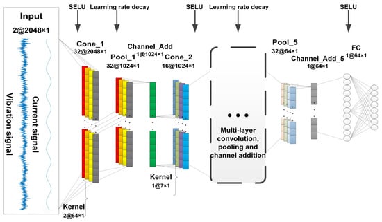
Figure 1.
The network structure of MC-DCNN.
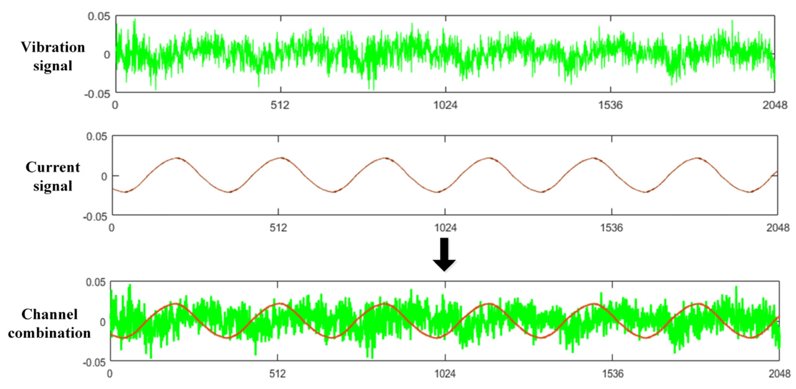
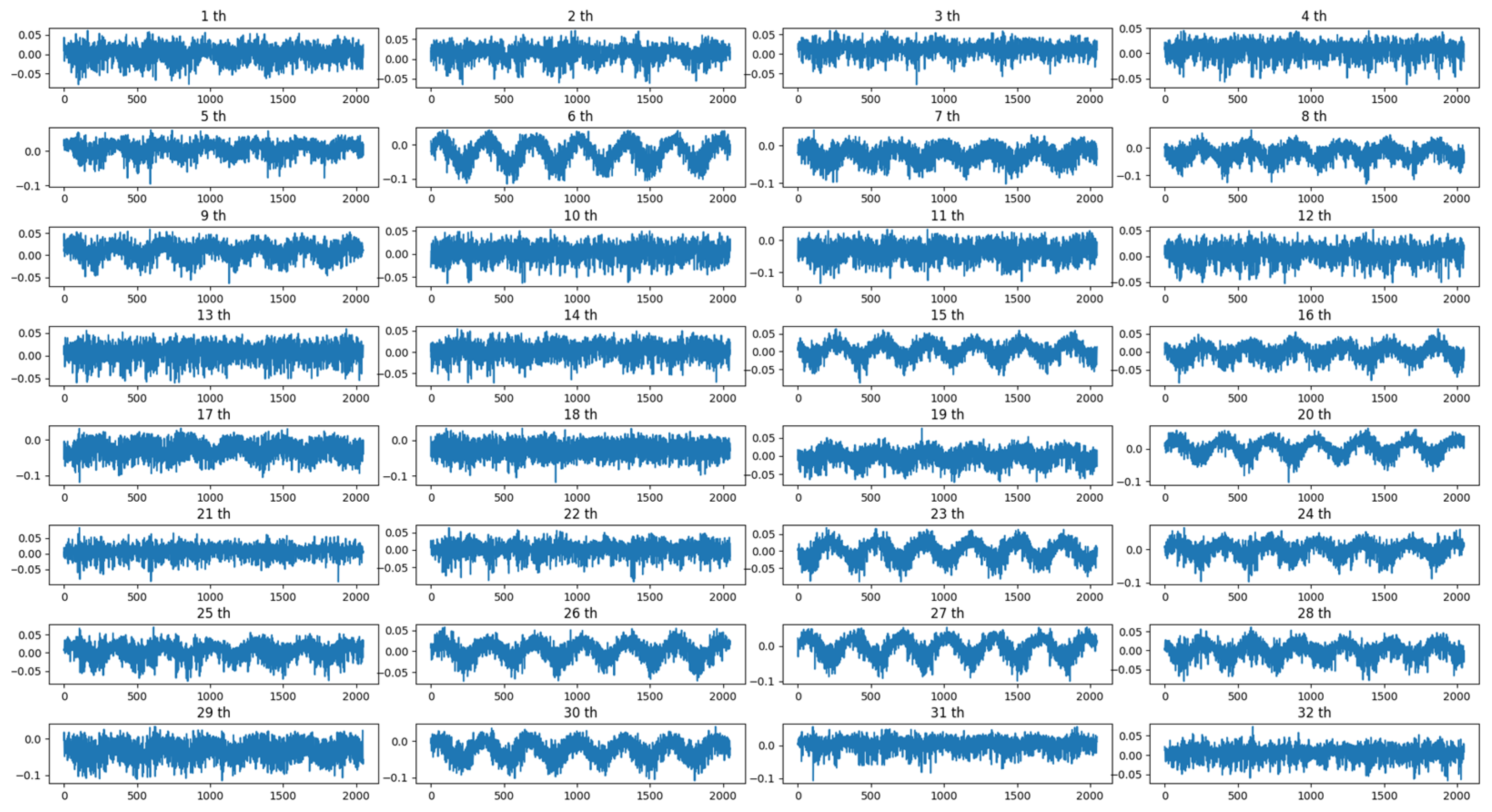
Multi-source signal input: The current and vibration signals are simply combined into two-channel data. As the information represented by vibration and current signals differs, the characteristics of the two datasets can be fused after the combined input operation (to the DCNN), and the fault information can be expressed more comprehensively. The use of 2048 × 1@2 dual-channel original vibration and current signals can better reflect the deep data mining capabilities of multi-input-source DCNN. For a clearer representation, the different signals obtained by the multi-source sensors are displayed in Figure 2.
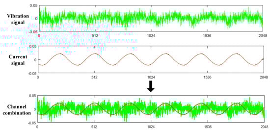
Figure 2.
Multi–source signal.
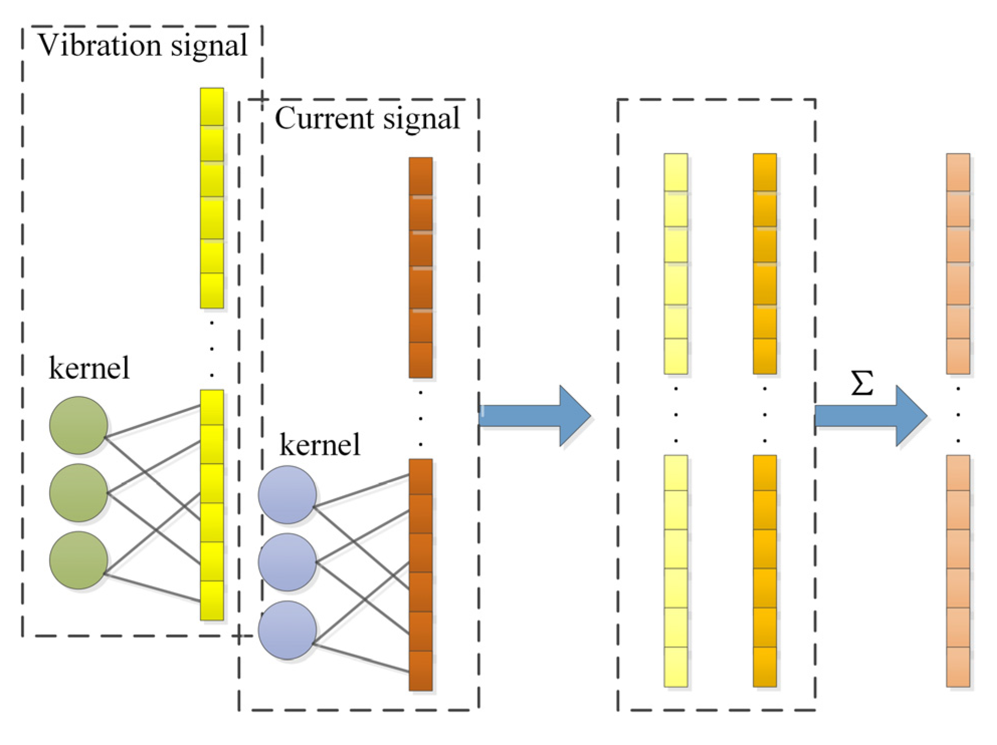
The convolutional layer: The one-dimensional convolution layers use one-dimensional convolution kernels to perform sliding convolution operations on the input one-dimensional data. Different convolution kernels generate different one-dimensional vectors for one-dimensional data convolution operations, and the same convolution kernel can share weights, reducing the number of calculations [24]. The network consists of five convolutional layers. The first layer has 32 convolution kernels with a size of 64 × 1, the second layer has 64 convolution kernels with a size of 7 × 1 and the third and fourth layers have 128 with a size of 7 × 1. The fifth layer has 32 convolution kernels with a size of 7 × 1. The data features are extracted by stacking multiple convolutional layers. When the multi-source signal is input to the DCNN, it goes to the multi-channel convolution kernel. As shown in the Figure 3, the double convolution kernel convolves the vibration and current signals separately, and then adds the convolution results to achieve information fusion. The one-dimensional convolution process can be expressed by the following equation.
where is the output of the l-th convolutional layer and is the number of channels. The convolutional layer is represented by the letter , and its number is . Conv1d is a one-dimensional convolution calculation in which the convolution calculation area is represented by and represents the i-th data. is the offset vector of the l − 1 layer of channel , and is the activation function of the l − 1 layer convolutional layer of channel .

Figure 3.
Multi-signal convolution process.
Pooling layer: The maximum pooling method is used to output the maximum value in the receptive field. The formula is shown in Equation (2) [25]. The pooling layer can achieve the purpose of data downsampling. The data in the network are reduced by one after each layer of pooling. The calculation time is greatly reduced after the pooling operation.
where is the output of the l-th pooling layer. The object of the receptive field in the layer is , and is the range of the receptive field.
Channel addition layer: Add the data vector obtained after convolution and pooling of multiple convolution kernels in each layer. After the addition, it becomes single-channel one-dimensional data. This operation can greatly reduce the number of calculations and achieve the purpose of information fusion again.
is the output after channel addition, which converts multi-dimensional features into one-dimensional vectors. p is the multi-dimensional feature vector after the previous layer pooling.
Fully-connected layer: Spread the features extracted after multiple layers of convolutional pooling into a one-dimensional vector. Each node in the fully-connected layer is fully connected to other nodes [26]. The formulas are as follows in Equations (4) and (5). Additionally, we use the softmax function to convert the output of the fully-connected layer into a probability distribution to classify the data.
where is the output calculated under the action of the activation function in the fully-connected layer. and are the weight and threshold of the i-th neuron, respectively, and is the output vector of the previous layer. In the softmax classifier, is the output value of the i-th node. C is the number of output nodes, which is the number of categories being classified.
Error back propagation: In the model, the output and are subjected to a cross-entropy operation with the actual label to obtain the loss function L, as shown in Equation (6). The chain derivation rule is used in the error back derivation of one-dimensional CNN, as in Equations (7) and (8). The error is propagated forward along each layer of the network and the network weight is updated.
where in the loss function is the i-th value in the actual vector and is the i-th value of the network output vector. In the formula, assuming that the error transmitted by the know convolutional layer is , then is the error of the previous hidden layer and the parameter that needs to be updated is .
2.2. SeLU Activation Function
The activation function uses nonlinear transformation to complete the nonlinear mapping of the data, which is different from the lack of expressive characteristics of the linear operation model, and it can improve the ability of the neural network to learn complex data. Using the activation function can better solve complex problems, efficiently learn data features and improve classification capabilities. In the process of CNN error backpropagation to update the parameters, a continuous multiplication formula of the activation function derivatives will appear. When the selected activation function is equal to 0, the problem of gradient disappearance will occur in the gradient descent, which causes the parameters in the upper network to be unable to update. When the derivative of the activation function is less than 0, the value after continuous multiplication of the derivative is also close to 0, which will cause the actual useful residual to become smaller early. Therefore, the activation function directly affects the convergence problem in the gradient descent process, and also directly affects the updating of the parameters and the learning efficiency of the network. The activation functions often used in neural network models include sigmoid, tanh, ReLU, Elu, Leacky-ReLU and SeLU, which are shown in Equations (9)–(13) [27].
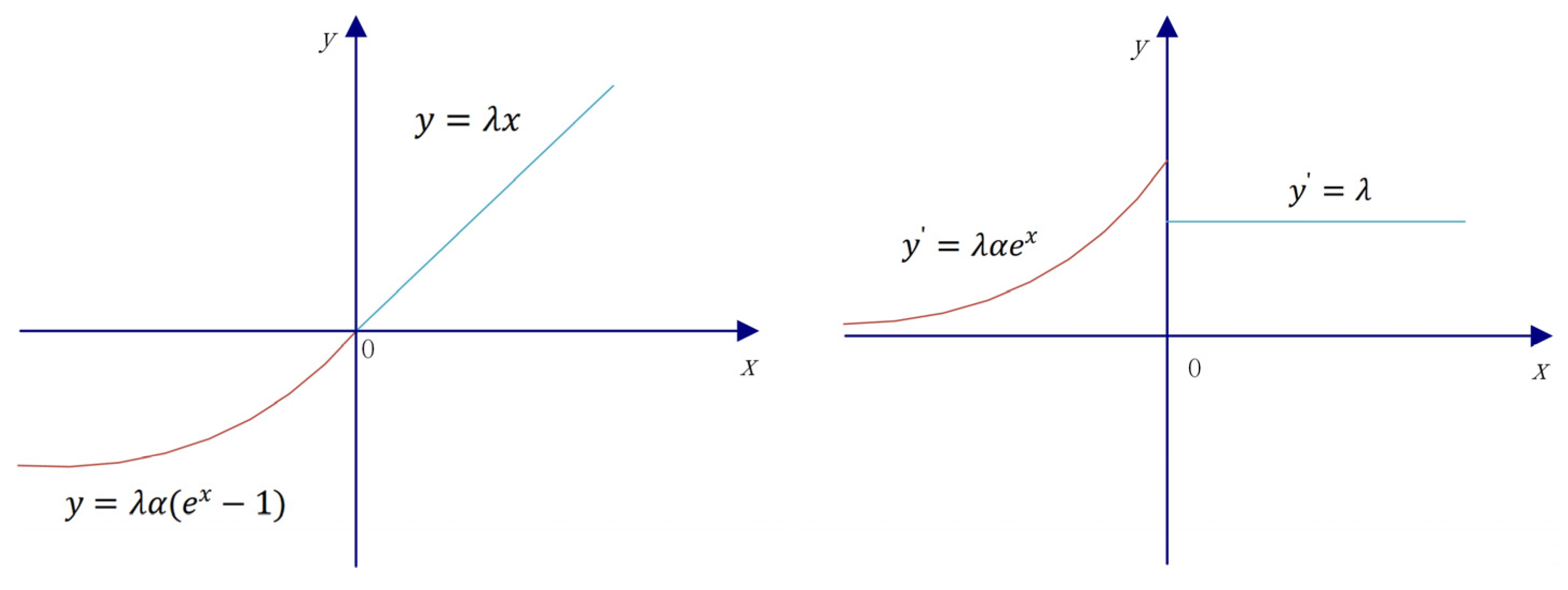
According to the formulas of these activation functions, it can be seen that the sigmoid function and tanh function are unsaturated linear functions, and the problems of gradient explosion and gradient disappearance cannot be avoided during model training, which will affect the convergence accuracy and speed models relying on them. The derivative of the formula for the ReLU activation function tells us that the derivative is equal to 1 when x is greater than 0, and 0 when the derivative is less than 0. When the derivative of the activation function is 1, the convergence speed is fast. However, when the derivative is 0, the dead point problem will appear, resulting in the error back propagation network parameters not being updated. The leaky-ReLU function is an improved ReLU function that is used to solve the problem that all negative information is lost. In the SeLU function, the value of is 1.6733 and the value of is 1.0507. Its function image and its derivative image are shown in Figure 4. When x is greater than 0, its derivative value is greater than 1 and it has a large closing velocity; when x is less than 0, its derivative value is not zero, and there is no gradient explosion or gradient vanishing problem. In addition, since SeLU has the property of normalization, its output is within the range of (0, 1), eliminating the steps of normalization processing in the model.
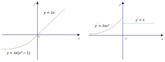
Figure 4.
The SELU activation function and its derivatives.
2.3. Adam Optimizer with Dynamic Attenuation Learning Rate
Adam is an improved gradient descent algorithm that can be used to update parameters in neural network models and is often used as an optimizer in the TensorFlow framework [28]. Equations (14)–(18) are used to illustrate the process of updating parameters with Adam.
where and represent the first-order moment gradient estimation and the second-order moment gradient estimation. The mean value and variance of the gradient can be used to control the parameter updating direction and learning rate of the neural network, respectively. and are the exponential decay rates of and , which are generally constants or default values close to 1, and is the gradient at the current time .
where and are the corrections of and with large initial deviations. When is large enough, the values of () and () are close to 1, so that the correction results reach the optimum.
This is the parameter update formula fir , where is the initial learning rate set. Additionally, is a minimal number that approaches 0, in order to prevent the denominator in the formula from being 0.
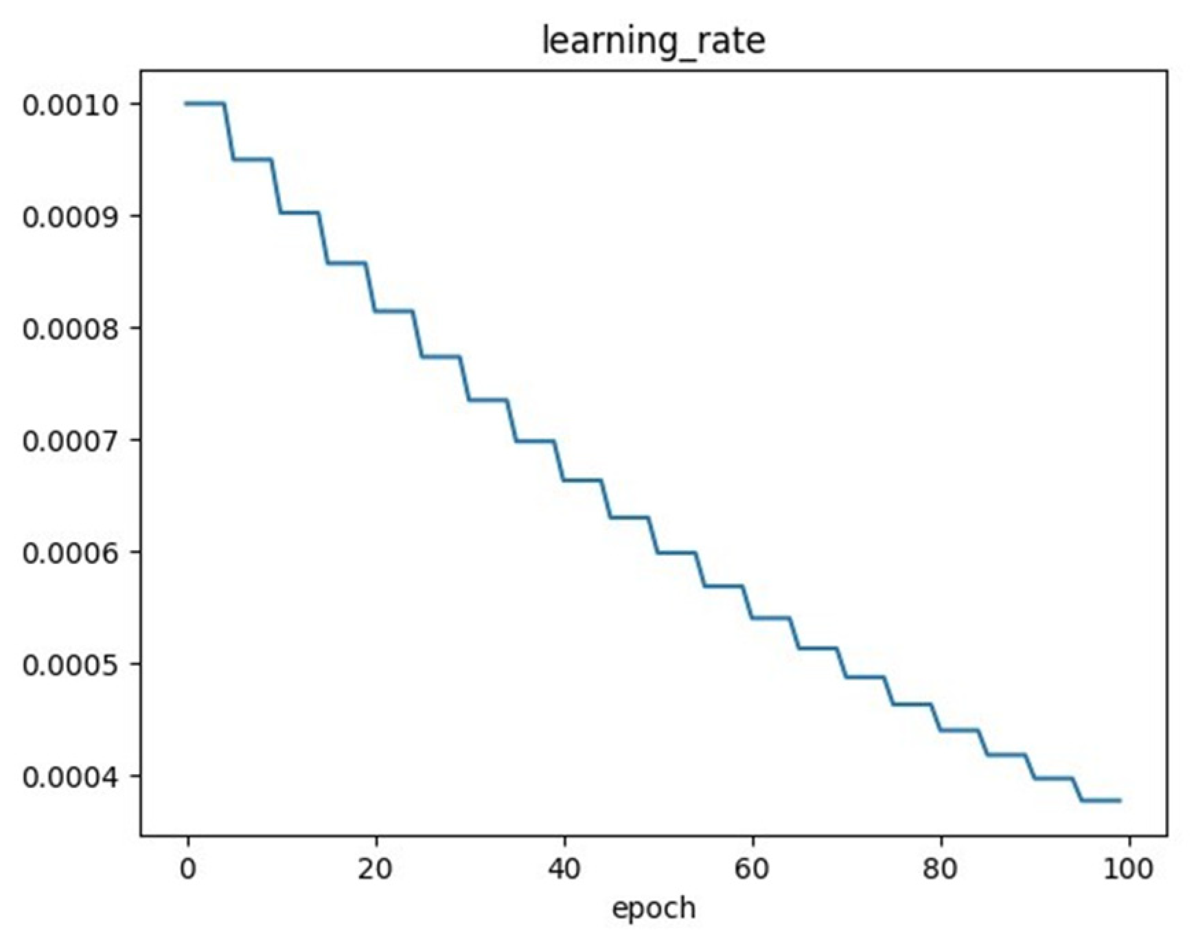
Custom attenuation learning rate can make the learning rate gradually decrease with the increase in iteration steps. As shown in Figure 5, 0.001 is taken as the initial learning rate. and five iterations are taken as the step size to attenuate. In the initial stage of model training, a large learning rate is needed to increase the training speed, but when the model is gradually approaching the optimum, the training pace should be reduced to ensure the accuracy of the training results. Additionally, the custom attenuation learning rate solves the two problems of model training speed and precision.
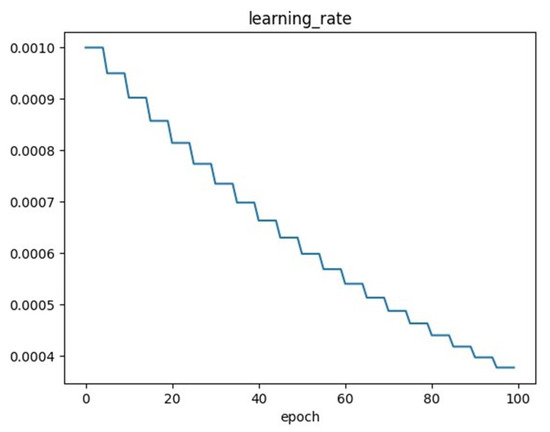
Figure 5.
Decay of the learning rate in model training.
Although Adam can adaptively change the learning rate to update the parameters, when the optimizer is given a fixed learning rate, Adam’s learning rate can only be capped by this fixed value to adapt to changes. If Adam is combined with the dynamic decaying learning rate, then this fixed value is no longer fixed. The upper limit of learning rate of Adam will decrease with the number of iteration steps, which ensures the convergence speed of the model while maintaining the stability and precision of convergence, and enables more efficient updating of parameters.
2.4. Data Augmentation Method
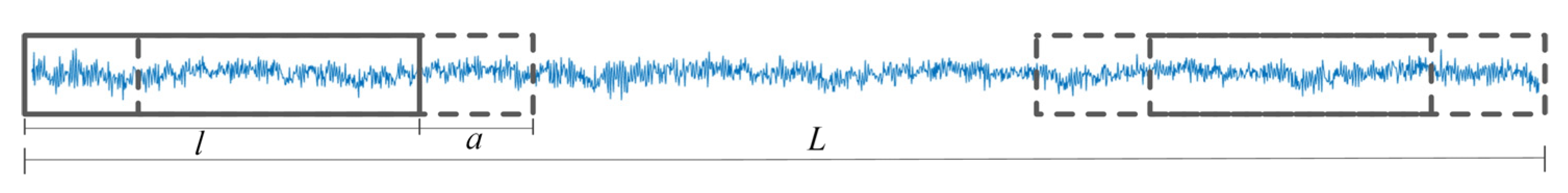
The fault diagnosis model based on deep learning needs a large number of data samples during training, but the samples of multi-fault coupling motor fault signals are not enough, and the data collected by the experimental bench cannot meet the training requirements of the model. The method of signal overlapping sampling can augment the dataset, which not only increases the diversity of samples but also effectively avoids overfitting [20]. The schematic diagram of the process of overlapping sampling of original data is shown in Figure 6.
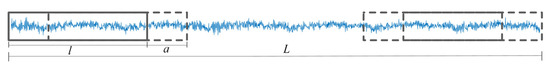
Figure 6.
Data overlap sampling process.
It can be seen in Figure 6 that the total length of a signal collected is L, and l represents the length of small sample signal to be intercepted. The size of each slide step during data resampling is a. Then, according to Equation (19), the number of samples n after data augmentation can be calculated, where 1 represents the mathematical symbol of rounding down.
3. MC-DCNN Fault Diagnosis Framework
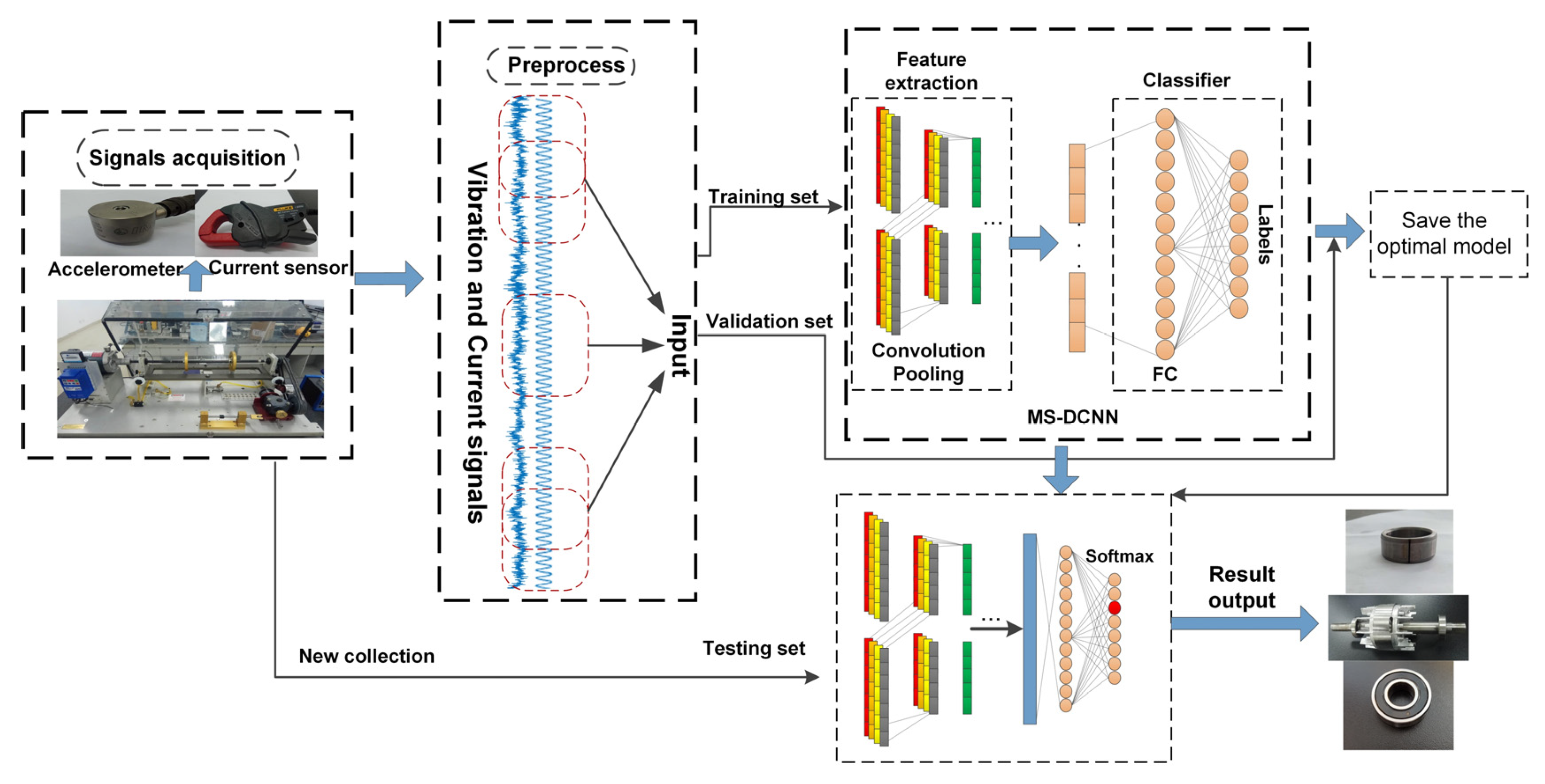
The multi-source signal fusion DCNN with improved super parameters for motor compound fault diagnosis process is shown in Figure 7. The following is a summary of the main steps of this method to realize the motor compound fault diagnosis process.

Figure 7.
Motor compound fault diagnosis process.
Step 1: We installed an acceleration sensor on the motor housing and installed a current clamp on the wire of the motor wiring cabinet, and then the vibration signal and current signal during the operation of the motor were collected through the data acquisition system.
Step 2: For the vibration signal and current signal, more samples were obtained by data augmentation method and divided into a training set and verification set.
Step 3: We built the model and set up the initial parameters, and then input the training set and validation set into a network model to update the model parameters.
Step 4: We saved the optimal model.
Step 5: We input the other newly acquired data into the trained model as the test set to identify the compound fault types.
4. Experiments and Results
4.1. Experimental Setting
In order to verify the applicability of the proposed method for motor compound fault diagnosis, the broken rotor bar fault, motor bearing faults and their compound faults were simulated by a comprehensive test bench of the motor and rotor system. The structure of the experimental platform is shown in Figure 8, which included a motor, rotating shaft, analog load system, acceleration sensor, current clamp, data acquisition system, etc. The acceleration sensor was installed on the motor shell, and the current clamp was installed on the wire of the motor wiring cabinet, the purposes of which were to obtain the vibration signal and to obtain the current signal under the running state of the motor. The current signals and vibration signals in each healthy state of the motor are collected at three motor speeds of 1196, 1789 and 2385 rpm, and the sampling frequency was 12,800 Hz.
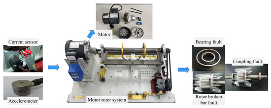
Figure 8.
Structure of the experimental platform.
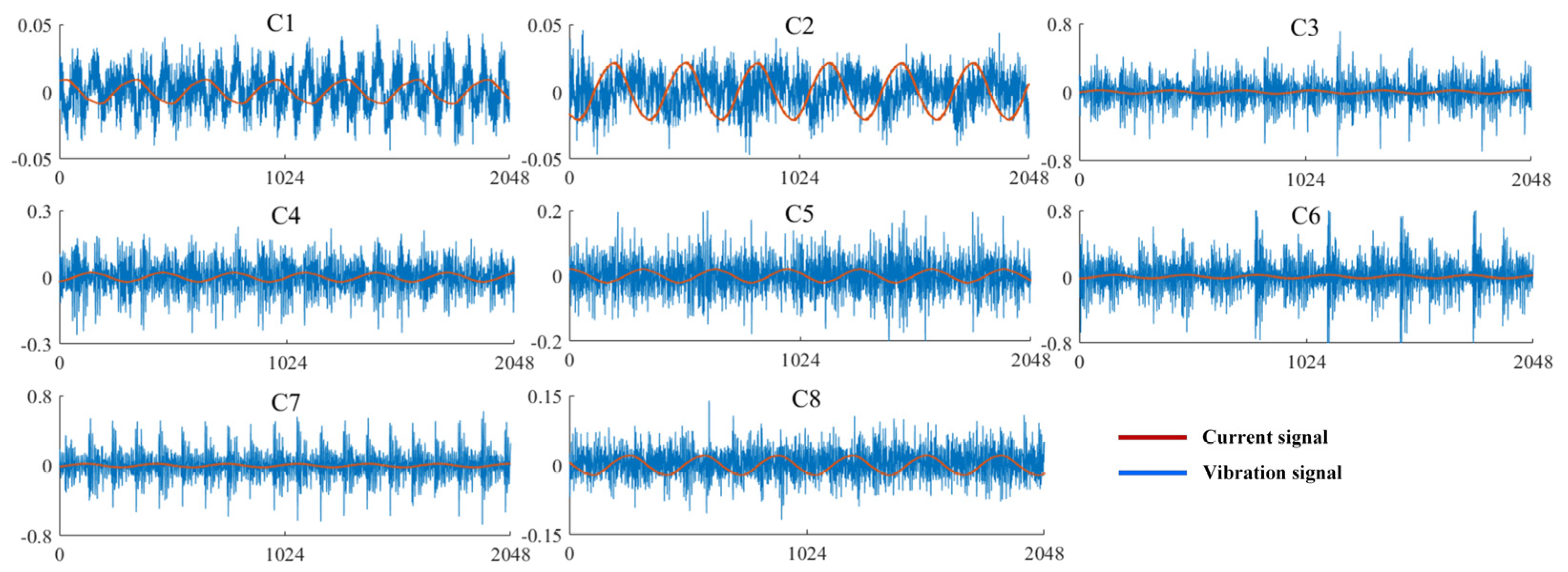
In the experiment, a U-shaped groove was milled out at the rotor’s end ring and guide bar, and the connection between the three guide bars and the end ring was cut off to simulate the broken bar fault. The motor bearing used in the experiment was a SKF6203 deep groove ball bearing, and defects were set at the inner ring, outer ring and rolling body of the bearing to simulate bearing failure. In order to verify the effectiveness of the proposed method for complex fault diagnosis for a motor, a total of eight working conditions of the motor were used in the experiment. They were normal (C1), broken rotor bar (C2), bearing inner ring fault (C3), bearing outer ring fault (C4), bearing rolling body fault (C5), compound fault including a broken rotor bar and bearing inner ring (C6), compound fault including a broken rotor bar and bearing outer ring (C7) and compound fault including a broken rotor bar and bearing rolling body (C8). The vibration and current signals of the eight kinds of faults at the actual motor speeds of 1196, 1789 and 2385 rpm were collected in the experiment, and 1000 samples with 2048 points for each fault were obtained at each speed. The dataset composed of 2 × 8000 × 2048 was divided into the training set (70%) and validation set (30%) for model training. Another 2 × 800 samples newly collected at the same speed were used as test sets. Figure 9 shows the two-channel waveforms of vibration and current signals in eight working states of the motor. Table 1 is a detailed description of the experimental dataset.
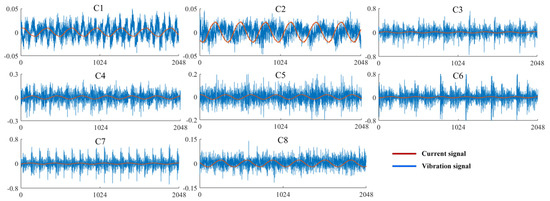
Figure 9.
Vibration and current signals from the motor under 8 working conditions.

Table 1.
Details of the experimental dataset.
The network structure and main parameters of multi-source signal fusion DCNN, including improved super parameters, are shown in Table 2. The network model can realize direct fault classification and diagnosis based on one-dimensional original signals. The inputs of the network are the current signal and vibration signal of the 2@2048 × 1 channels. The first convolution layer uses the large size of 64 × 1 convolution kernel to effectively remove noise and reduce the burden of network computation. Multiple convolutional layers containing 7 × 1 small convolutional kernels are stacked into a deep network, which can mine data features more accurately. In the process of network training, the SELU activation function and learning rate of dynamic attenuation were used to improve the network’s hyperparameters.
Table 2.
The main structural parameters of the MC-DCNN model.
4.2. Motor Compound Fault Diagnosis
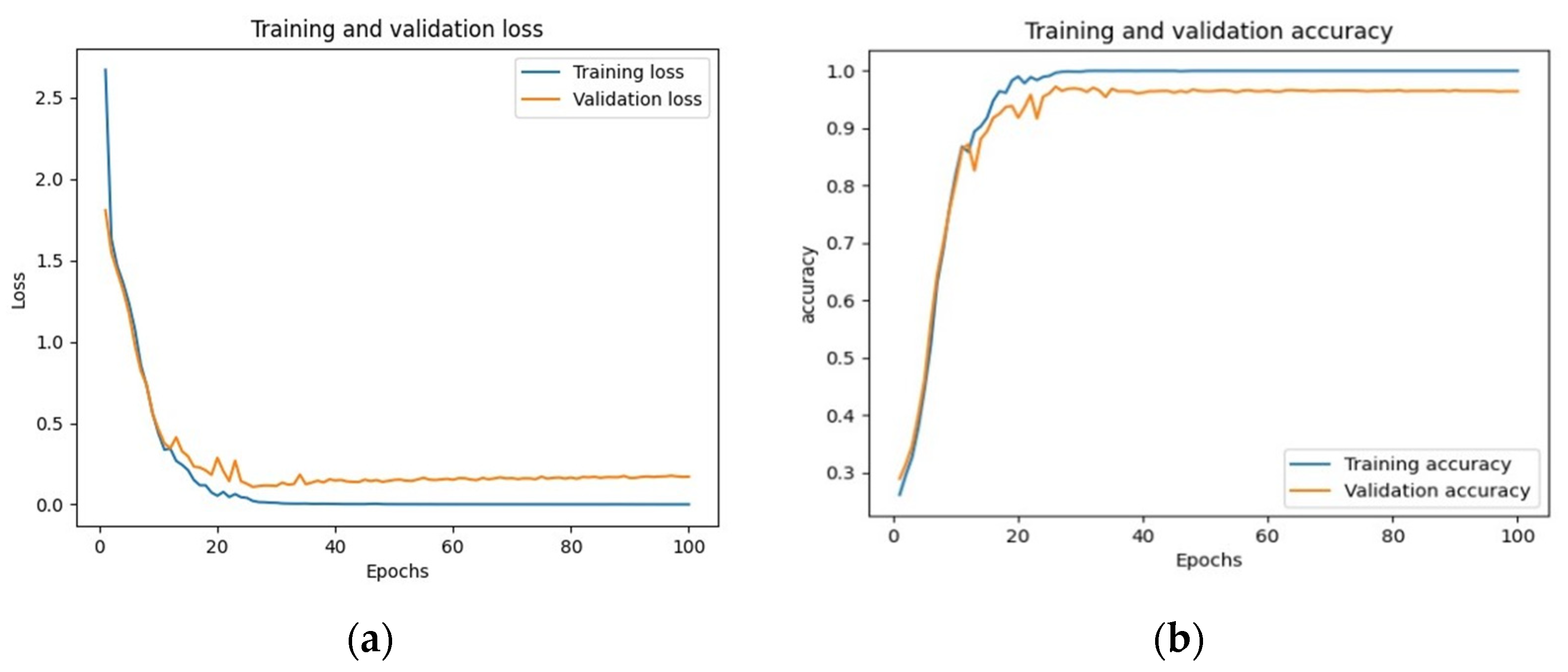
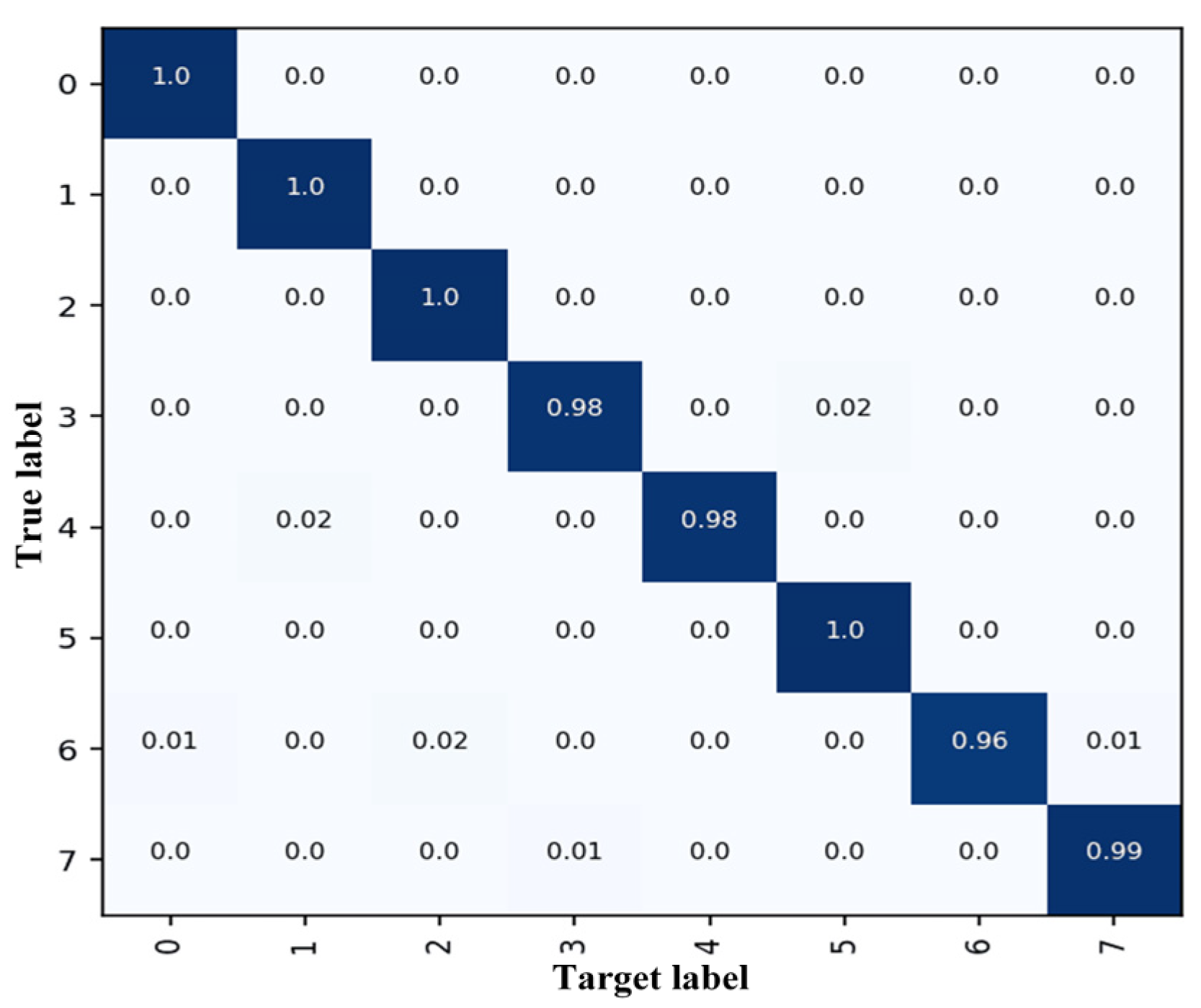
Firstly, the experimental signals collected at 1789 r/min of compound faults were analyzed and verified by using the MC-DCNN model, and the original vibration and current signals of the motor were taken as the inputs of the model. The number of iterations was set to 100 during model training, and the training set and verification set described above were used to verify the model, and the model with the highest accuracy during verification was saved as the optimal model. Figure 10 shows the convergence curve of the model during training, and it can be seen that it gradually converged on the optimum and was stable. Then, the newly collected signals of other motors at the speed of 1789 rpm were used as the test set of the model. Figure 11 shows the confusion matrix of sample accuracy on the test set of eight motor health states. It can be seen in categories C6, C7 and C8 that the model has excellent compound fault identification.
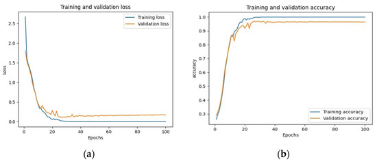
Figure 10.
Convergence curves of the model under the action of the training set and test set: (a) loss; (b) accuracy.
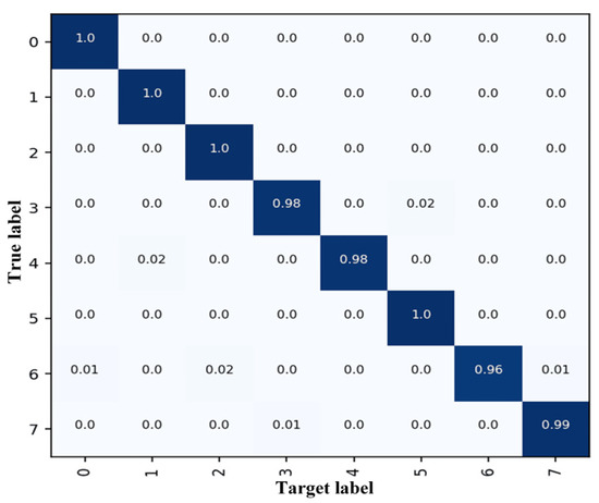
Figure 11.
Confusion matrix of recognition rate.
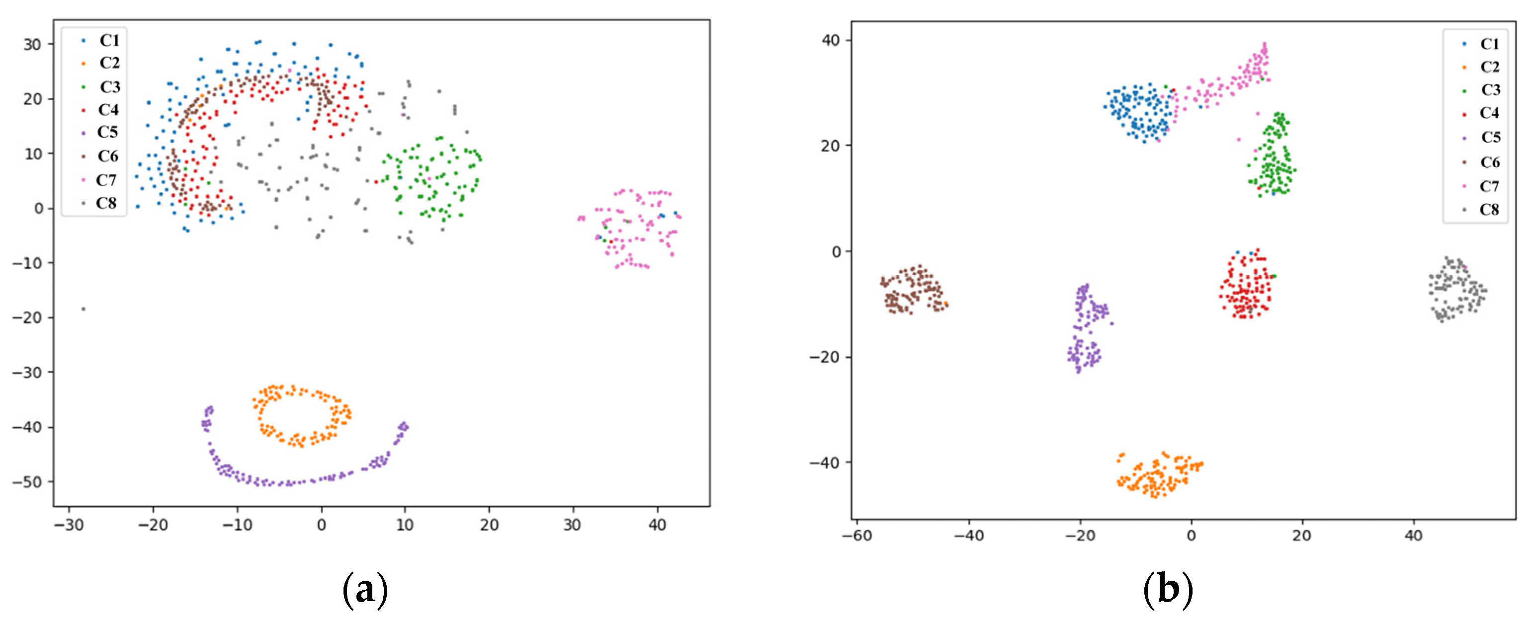
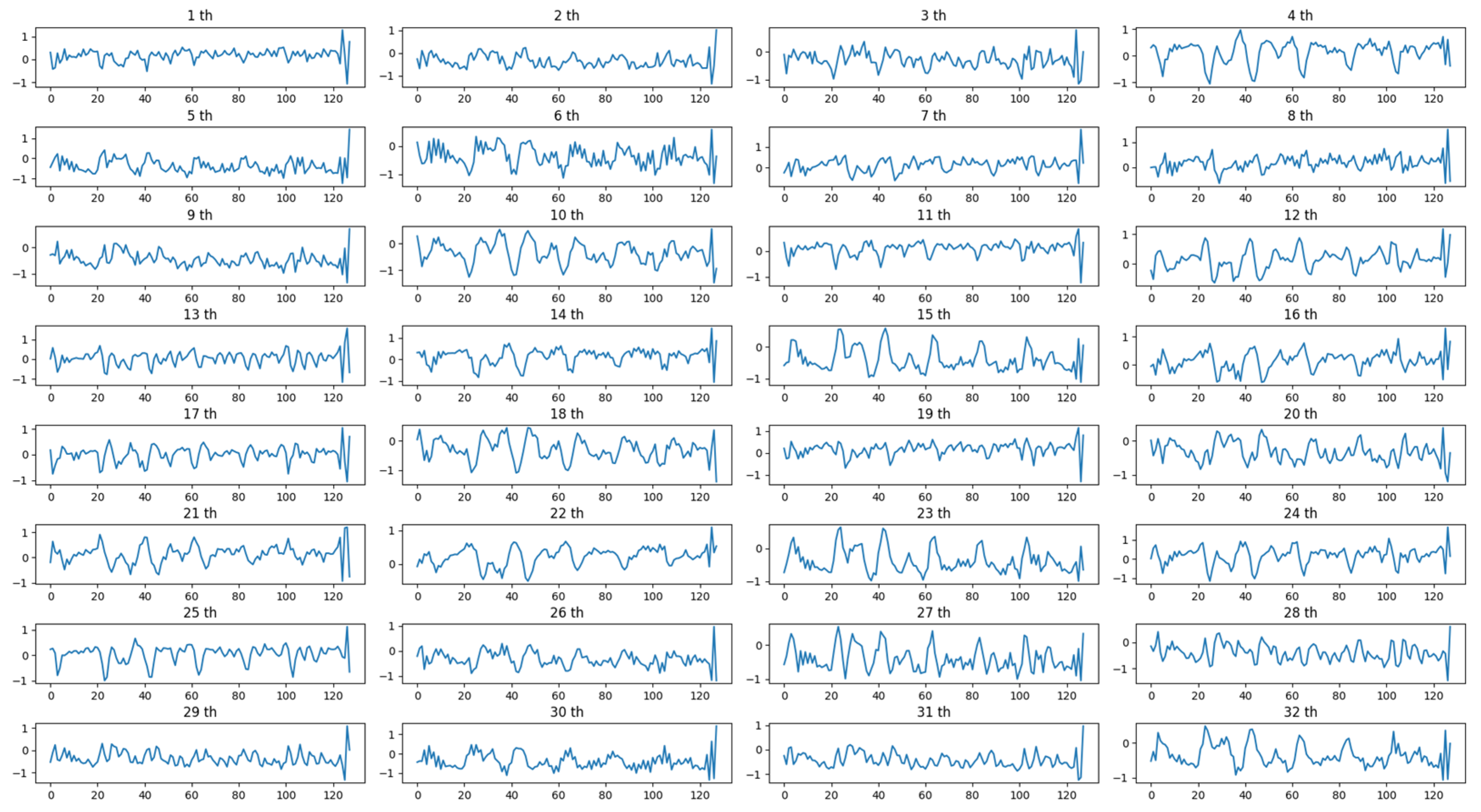
In order to demonstrate the internal working principle of the deep network model more clearly, the feature extraction process of the multi-source signal DCNN model is analyzed visually. T-distributed stochastic neighbor embedding (T-SNE) is a common method for data dimension reduction and visualization analysis. Figure 12 shows the feature distribution of data through the first-layer convolutional pooling and the fifth-layer convolutional pooling. It can be seen in the figure that the classification characteristics of data became gradually obvious after multi-layer stacked convolutional pooling. In each convolution layer of the model, convolution kernels of different shapes but a particular size were randomly generated. These convolution kernels are like many filters for multiple filtering of the signal, in order to extract features in the signal comprehensively and deeply. Figure 13 and Figure 14 show the vector output waveforms after the convolution of the signal at the first and fifth layers, respectively. It can be seen that the vector waveform after the convolution at the first layer retained the waveform features of the original data, but after the deep convolution in the fifth layer, it only retained the useful features of the signal that were clearer. Additionally, because of the SeLU activation function’s need to avoid the dead point problem, every convolution kernel played a role in extracting useful features.
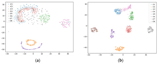
Figure 12.
Clustering effect of different convolution layers under T-SNE: (a) first layer; (b) fifth layer.
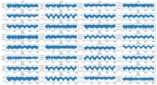
Figure 13.
Feature vector output of the first convolution layer.
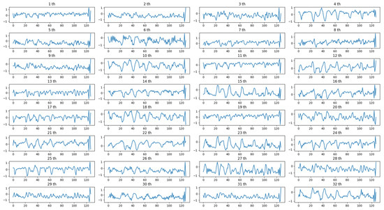
Figure 14.
Feature vector output of the fifth convolution layer.
The applicability of the proposed model to compound fault diagnosis of our motor various working conditions was further verified, and the current and vibration signal data were analyzed at 1196 and 2385 rpm, respectively. Just like the above process, the training set was used to train the model, and the optimal model was picked according to the highest accuracy on the verification set. Then the newly collected test set data were sent into the model for identification and verification. Finally, through several experiments on the model, the statistical graph of fault identification accuracy was obtained, as shown in Figure 15, which includes the identification accuracy and average accuracy for all eight motor health states at three speeds of 1196, 1789 and 2385 rpm. As can be seen in Figure 15, the fault identification accuracy of the model for motor compound faults at three speeds was more than 98.35%.
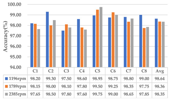
Figure 15.
The recognition accuracy for each health condition.
4.3. Comparison and Discussion
In order to further verify the superiority of the improved hyperparameter MC-DCNN model, three groups of comparative experiments were designed. The first set of experiments used a single signal of current or vibration as the model input to verify the validity of the model based on multi-source signals. In the second group of experiments, the model trained with decayed learning rate was compared with the model trained with a fixed and undecayed learning rate. The third set of experiments compared the effect of the model using the SeLU activation function with the effect of the model using the ReLU activation function. The second and third experiments were the verification of the improved hyperparameters’ effect on the MC-DCNN model.
- (1)
- Comparison of single-signal and multi-signal fault diagnosis
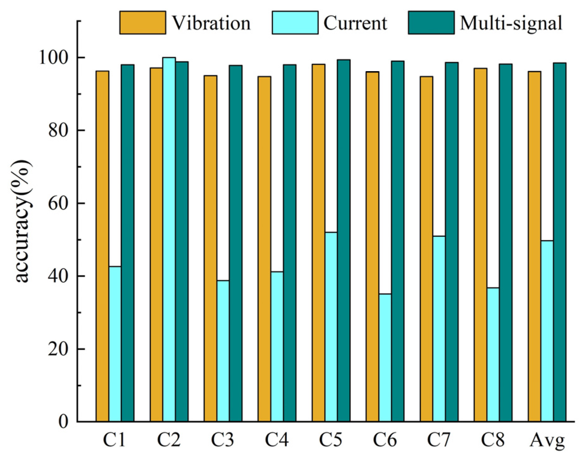
The characteristic information contained in the data collected by different types of sensors is often different. This experiment analyzed the fault classification accuracy of the DCNN model based on a single vibration signal or current signal, and the fault classification accuracy of the MC-DCNN model based on vibration and current signal. The current signals and vibration signals of the same eight motor health conditions, as described above, were collected, and the signals were pretreated with the same operation to get 8×1000 small samples of each motor health condition. Five experiments were carried out with single signals and multiple signals, and the average classification accuracy of each type of defect and the overall average accuracy were recorded. The results are recorded in Table 3 and Figure 16.
Table 3.
DCNN classification accuracy based on single signals and the multi-signal.

Figure 16.
Classification accuracy of different types of signals in eight motor health conditions.
As can be seen in Table 3, the average accuracy for the eight types of health conditions based on vibration signals was 96.13%, and the average accuracy based on current signals was very low. However, it is worth noting that the fault identification rate for C2 (motor rotor bar breaking) reached 100%, indicating that the current signals contain obvious bar breaking fault characteristics. The average fault diagnosis accuracy of multi-signal data was 98.48%, which is about 2% higher than that of using the vibration signals alone. This shows that the MC-DCNN model has great advantages for compound fault diagnosis.
- (2)
- Comparative experiment of SeLU and ReLU in MC-DCNN
In the training of the MC-DCNN model, the SeLU activation function and ReLU activation function were selected, and the same test set data were used for the experimental comparison of fault classification. During model evaluation, precision rate, recall rate, F1-score and average accuracy were used as evaluation indexes of the model, and the results are shown in Table 4. The signals of C6, C7 and C8 compound fault types were selected as the experimental test set data. The results show that the model’s accuracy when trained by the SeLU activation function was improved compared with that of the model with a ReLU activation function, according to various evaluation indexes, and the average accuracy was increased by 7.34%. The comparison shows that the model trained by the SeLU activation function had higher classification accuracy.
Table 4.
Evaluation index of MC-DCNN based on different activation functions.
- (3)
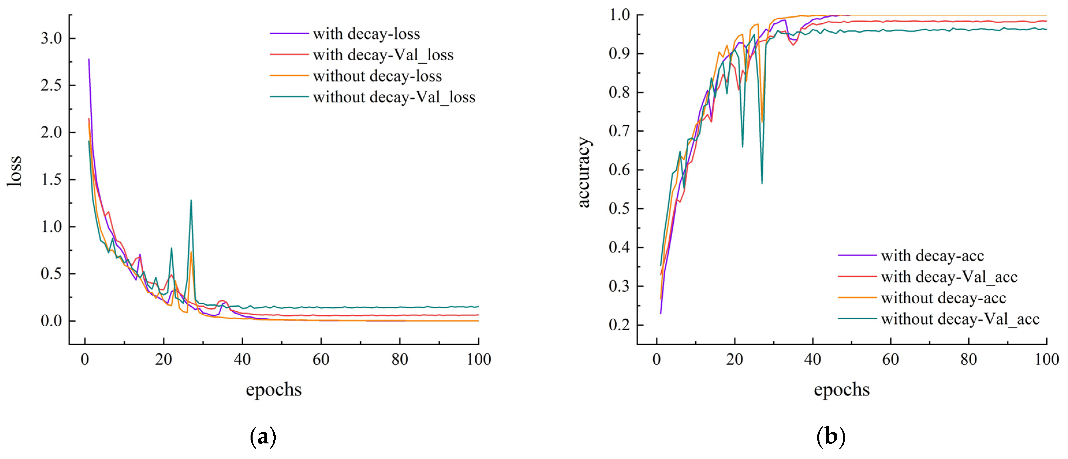
- Comparative experiment of learning rate with decay and without decay in MC-DCNN
The learning rate can affect the accuracy and convergence efficiency of the model in model training. The learning rate with dynamic decay was combined with the Adam algorithm to optimize the model. In order to verify the effectiveness of this method, the experiment used a fixed learning rate without decay for comparison. The initial learning rate was set to 0.001, and five experiments were conducted to calculate the average losses and accuracies in the processes of model training and verification. The losses and accuracies of the two learning rate models on the training set and verification set are shown in Figure 17, and the comparative statistical results are shown in Table 5.
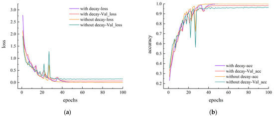
Figure 17.
Convergence curves of the model at fixed and decaying learning rates: (a) loss; (b) accuracy.
Table 5.
Comparison of model effects based on different learning rates.
It can be clearly seen in Figure 17 that the convergence curve of the model with attenuation learning rate training is more stable, whereas the model with fixed learning rate experienced a large oscillation in convergence. As can be seen in the statistical data for validation set listed in Table 5, compared with the fixed learning rate, the accuracy of the attenuation learning rate was increased by 2.18%, and the loss value was reduced by 0.0905. It is shown that using the learning rate with decay to train the model can reduce the convergence error and improve the convergence stability of the model, and at the same time improve the recognition accuracy of the model for complex faults.
5. Conclusions
In this paper, the MC-DCNN model was proposed. It uses multi-source signals to realize fault diagnosis of a motor with compound faults. The model is applied to the original vibration signal and current signal of the motor, which can fully integrate and extract the fault features contained in different signals. Moreover, the hyperparameter optimization of the MC-DCNN model is carried out by using the SELU activation function and attenuation learning rate. The experiment proved that the SELU activation function can effectively avoid the “dead point” problem in model training, and the combination of dynamic attenuation learning rate and the Adam algorithm can improve the convergence stability of the model and the classification accuracy of the model. Finally, through three types of comparative experimental analysis, it was proved that the improved hyperparameter MC-DCNN model proposed in this paper is effective for multi-source signal information fusion and feature extraction.
In future studies, this method could be applied to different fault diagnosis objects. DCNN can be used as a tool for fault feature extraction and multi-source signal feature fusion, and it can be combined with other fault diagnosis and classification algorithms.
Author Contributions
Conceptualization, X.G. and Z.Z.; methodology, W.D.; software, Z.Z.; validation, Z.Z., K.F. and T.W.; formal analysis, Z.Z.; investigation, K.F.; resources, X.G.; data curation, W.D.; writing—original draft preparation, Z.Z.; writing—review and editing, X.G.; visualization, K.F.; supervision, W.D.; project administration, X.G.; funding acquisition, X.G. All authors have read and agreed to the published version of the manuscript.
Funding
This research was funded in part by the National Natural Science Foundation of China (approved grant: U1804141), in part by Foundation for University Key Teacher of Henan Educational Department (2018GGJS091), and in part by Science and Technology Program of Henan, China (222102220081).
Data Availability Statement
Not applicable.
Acknowledgments
Many thanks to editors and reviewers for their comments and help.
Conflicts of Interest
The authors declare no conflict of interest.
References
- Shi, P.; Chen, Z.; Vagapov, Y.; Zouaoui, Z. A new diagnosis of broken rotor bar fault extent in three phase squirrel cage induction motor. Mech. Syst. Signal Process. 2014, 42, 388–403. [Google Scholar] [CrossRef]
- Gangsar, P.; Tiwari, R. Signal based condition monitoring techniques for fault detection and diagnosis of induction motors: A state-of-the-art review. Mech. Syst. Signal Process. 2020, 144, 106908. [Google Scholar] [CrossRef]
- Chen, X.; Wang, S.; Qiao, B.; Qiang, C. Basic research on machinery fault diagnostics: Past, present, and future trends. Front. Mech. Eng. 2018, 13, 264–291. [Google Scholar] [CrossRef] [Green Version]
- Delgado-Arredondo, P.A.; Morinigo-Sotelo, D.; Osornio-Rios, R.A.; Avina-Cervantes, J.G. Methodology for fault detection in induction motors via sound and vibration signals. Mech. Syst. Signal Process. 2017, 83, 568–589. [Google Scholar] [CrossRef]
- Wu, Y.; Jiang, B.; Wang, Y. Incipient winding fault detection and diagnosis for squirrel-cage induction motors equipped on CRH trains. ISA Trans. 2020, 99, 488–495. [Google Scholar] [CrossRef] [PubMed]
- Tian, M.; Li, S.; Song, J.; Lin, L. Effects of the mixed fault of broken bars and static eccentricity on current of induction motor. Electr. Mach. Control 2017, 21, 1–9. [Google Scholar]
- Gu, F.; Shao, Y.; Hu, N.; Naid, A.; Ball, A.D. Electrical motor current signal analysis using a modified bispectrum for fault diagnosis of downstream mechanical equipment. Mech. Syst. Signal Process. 2011, 25, 360–372. [Google Scholar] [CrossRef]
- Zhen, D.; Wang, T.; Gu, F.; Ball, A.D. Fault diagnosis of motor drives using stator current signal analysis based on dynamic time warping. Mech. Syst. Signal Process. 2013, 34, 191–202. [Google Scholar] [CrossRef] [Green Version]
- He, Z.J.; Wu, F.; Chen, B.Q. Automatic fault feature extraction of mechanical anomaly on induction motor bearing using ensemble super-wavelet transform. Mech. Syst. Signal Process. 2015, 54–55, 457–480. [Google Scholar] [CrossRef]
- Jing, S.; Zhao, X.; Guo, S.; Wang, Z. Fault diagnosis research of asynchronous motor rotor broken bar. J. Henan Polytech. Univ. (Nat. Sci.) 2016, 35, 224–229. [Google Scholar]
- Camarena-Martinez, D.; Osornio-Rios, R.; Romero-Troncoso, R.J. Fused Empirical Mode Decomposition and MUSIC Algorithms for Detecting Multiple Combined Faults in Induction Motors. J. Appl. Res. Technol. 2015, 10, 160–167. [Google Scholar] [CrossRef]
- Lei, Y.; Yang, B.; Jiang, X.; Jia, F.; Nandi, A.K. Applications of machine learning to machine fault diagnosis: A review and roadmap. Mech. Syst. Signal Process. 2020, 138, 106587. [Google Scholar] [CrossRef]
- Mao, W.; Feng, W.; Liu, Y.; Zhang, D.; Liang, X. A new deep auto-encoder method with fusing discriminant information for bearing fault diagnosis. Mech. Syst. Signal Process. 2021, 150, 107233. [Google Scholar] [CrossRef]
- Wang, S.; Xiang, J.; Zhong, Y.; Tang, H. A data indicator-based deep belief networks to detect multiple faults in axial piston pumps–Science Direct. Mech. Syst. Signal Process. 2018, 112, 154–170. [Google Scholar] [CrossRef]
- Zhang, Y.; Zhou, T.; Huang, X.; Cao, L.; Zhou, Q. Fault diagnosis of rotating machinery based on recurrent neural networks. Measurement 2020, 171, 108774. [Google Scholar] [CrossRef]
- Sony, S.; Dunphy, K.; Sadhu, A.; Capretz, M. A systematic review of convolutional neural network-based structural condition assessment techniques. Eng. Struct. 2021, 226, 111347. [Google Scholar] [CrossRef]
- Choudhary, A.; Mian, T.; Fatima, S. Convolutional Neural Network Based Bearing Fault Diagnosis of Rotating Machine Using Thermal Images. Measurement 2021, 176, 109196. [Google Scholar] [CrossRef]
- Liang, P.; Deng, C.; Wu, J.; Yang, Z.X. Intelligent fault diagnosis of rotating machinery via wavelet transform, generative adversarial nets and convolutional neural network. Measurement 2020, 159, 107768. [Google Scholar] [CrossRef]
- Wei, Z.; Li, C.; Peng, G.; Chen, Y.; Zhang, Z. A deep convolutional neural network with new training methods for bearing fault diagnosis under noisy environment and different working load. Mech. Syst. Signal Process. 2017, 100, 439–453. [Google Scholar]
- Gao, S.; Pei, Z.; Zhang, Y.; Li, T. Bearing fault diagnosis based on adaptive convolutional neural network with nesterov momentum. IEEE Sens. J. 2021, 21, 9268–9276. [Google Scholar] [CrossRef]
- Shi, J.; Yi, J.; Ren, Y.; Li, Y.; Chen, L. Fault diagnosis in a hydraulic directional valve using a two-stage multi-sensor information fusion. Measurement 2021, 179, 109460. [Google Scholar] [CrossRef]
- Jing, L.; Wang, T.; Ming, Z.; Peng, W. An Adaptive Multi-Sensor Data Fusion Method Based on Deep Convolutional Neural Networks for Fault Diagnosis of Planetary Gearbox. Sensors 2017, 17, 414. [Google Scholar] [CrossRef] [PubMed] [Green Version]
- Shao, S.; Yan, R.; Lu, Y.; Wang, P.; Gao, R.X. DCNN-Based Multi-Signal Induction Motor Fault Diagnosis. IEEE Trans. Instrum. Meas. 2020, 69, 2658–2669. [Google Scholar] [CrossRef]
- Lu, Y.; Lu, G.; Zhou, Y.; Li, J.; Xu, Y.; Zhang, D. Highly shared Convolutional Neural Networks. Expert Syst. Appl. 2021, 175, 114782. [Google Scholar] [CrossRef]
- Boureau, Y.L.; Bach, F.; Lecun, Y.; Ponce, J. Learning Mid-Level Features for Recognition. In Proceedings of the 2010 IEEE Computer Society Conference on Computer Vision and Pattern Recognition, San Francisco, CA, USA, 13–18 June 2010; pp. 2559–2566. [Google Scholar]
- Sindi, H.; Nour, M.; Rawa, M.; Öztürk, Ş.; Polat, K. Random Fully Connected Layered 1D CNN for Solving the Z-Bus Loss Allocation Problem. Measurement 2021, 171, 108794. [Google Scholar] [CrossRef]
- Clevert, D.A.; Unterthiner, T.; Hochreiter, S. Fast and accurate deep network learning by exponential linear units (elus). arXiv 2016, arXiv:1511.07289. [Google Scholar]
- Kingma, D.P.; Ba, J.L. Adam: A method for stochastic optimization. arXiv 2015, arXiv:1412.6980. [Google Scholar]


Publisher’s Note: MDPI stays neutral with regard to jurisdictional claims in published maps and institutional affiliations. |
© 2022 by the authors. Licensee MDPI, Basel, Switzerland. This article is an open access article distributed under the terms and conditions of the Creative Commons Attribution (CC BY) license (https://creativecommons.org/licenses/by/4.0/).