Abstract
This paper investigates the numerical integration error calibration problem in Lie group sigma point filters to obtain more accurate estimation results. On the basis of the theoretical framework of the Bayes–Sard quadrature transformation, we first established a Bayesian estimator on matrix Lie groups for system measurements in Euclidean spaces or Lie groups. The estimator was then employed to develop a generalized Bayes–Sard cubature Kalman filter on matrix Lie groups that considers additional uncertainties brought by integration errors and contains two variants. We also built on the maximum likelihood principle, and an adaptive version of the proposed filter was derived for better algorithm flexibility and more precise filtering results. The proposed filters were applied to the quaternion attitude estimation problem. Monte Carlo numerical simulations supported that the proposed filters achieved better estimation quality than that of other Lie group filters in the mentioned studies.
1. Introduction
Estimating the state of dynamical systems is a research hotspot and a frequently faced essential issue in many real-life applications, e.g., navigation, target tracking, robotics, and automatic control [1,2,3]. Due to the imperfect system model and the existence of noise, filtering is the most used estimating approach. For linear systems with Gaussian uncertainties, the Kalman filter (KF) [4], as the most desirable estimator established on minimal mean-square-error (MMSE) criterion, can provide an optimal recursive solution. However, while the system is nonlinear, obtaining the optimal closed-form solution is intractable. Researchers proposed various methods via analytical or numerical approximation to address nonlinear state estimation issues. A successful analytical approximation method is the extended Kalman filter (EKF) [5], which employs first-order Taylor series approximation to linearize nonlinear dynamics, but may perform poorly with highly nonlinear systems or large initial errors. Moreover, the main drawback of the EKF is that it needs to calculate the Jacobians, which is relatively tricky for complicated models.
Instead of dealing with nonlinearities by evaluating Jacobians, another class of nonlinear filtering based on numerical approximation is preferred. These filters are collectively called sigma point filters, including the unscented Kalman (UKF) [6], Gauss–Hermite–Kalman (GHKF) [7], and cubature Kalman (CKF) [8] filters. Different deterministic sigma points are used in these filtering algorithms to approximate moments of the probability distribution functions (PDFs). Compared with the EKF, the sigma point Kalman filter can provide better robustness and estimation accuracy, but increases the computational burden. Another problem underlying the sigma point Kalman filter is that errors caused by the traditional numerical quadrature rules may inject bias into the estimated moments without compensation. Concerning that ignoring the integral approximation error may lead to overconfident estimates, several studies employed Bayesian quadrature (BQ) and other quadrature approaches based on BQ theory (such as Gaussian process quadrature (GPQ) and Bayes–Sard quadrature (BSQ)) to improve the sigma point Kalman filter [9,10,11]. These approaches are successful because BQ, GPQ, and BSQ rules can quantify uncertainty in numerical integration.
Most EKFs and sigma point Kalman filters are designed for system dynamical models in Euclidean spaces in the existing literature. Nevertheless, when the system state exists in a Riemannian manifold, considering the geometry of the manifold can have merits, for example, enlarging the convergence domain and increasing the convergence rate [12]. Many works are devoted to introducing Euclidean space filters to manifolds to obtain natural and good metrics. The authors in [13] generalized the unscented transform and the UKF to Riemannian manifolds, and produced a general optimization framework. By extending the main concepts of UKF for Riemannian state-space systems, the authors in [14] proposed a series of more widespread and consistent Riemannian UKFs (RiUKFs) that supplement the theory gap in UKF on manifolds. Another generalized method about UKF on manifolds was presented in [15], which further developed the authors’ previous work of UKF on Lie groups in [16,17].
Implementing KFs on Lie groups is another widely studied line of designing filtering algorithms on manifolds, which was first proposed in [18,19]. Due to the systems’ invariance properties, many studies proposed invariant KFs on Lie groups: the authors in [20,21,22,23] designed intrinsic continuous-discrete invariant EKFs (IEKFs) for continuous-time systems on Lie groups with discrete-time measurements in Euclidean spaces and applied them to attitude estimation and inertial navigation; in [24,25,26], the researchers proposed the invariant UKFs (IUKFs). To help practitioners fully understand IEKFs, Ref. [27] provided three typical examples, and [28] presented the right IEKF algorithm for simultaneous localization and mapping (SLAM). Moreover, the authors in [29,30,31,32] devised EKFs on Lie groups for systems with measurements on matrix Lie groups. Other designs proposed EKF extensions for Lie groups [12,33]. On the other hand, UKF on Lie groups (UKF-LG) was developed in [16,17] for SLAM and sensor fusion. The authors in [34] suggested an impressive UKF based on UKF theory on Lie groups for visual–inertial SLAM. Unlike UKF-LG, in [35], the authors proposed another type of UKF filter for matrix Lie groups. This filter takes the time propagation step on the Lie algebra, improving computation efficiency. In addition, the authors in [36] introduced an invariant CKF on Lie groups for the attitude estimation problem from vector measurements.
Even if the above works succeeded in extending the sigma point filters to the Lie group, these filters still do not consider integration errors caused by quadrature rules. Hence, this paper is concentrated on calibrating the numerical integration error in the sigma point filtering algorithm on matrix Lie groups to improve filtering estimation quality. Motived by the previous study on employing the Bayes–Sard quadrature (BSQ) method in Euclidean sigma point filtering, we attempted to extend the BSQ method to filters on matrix Lie groups. According to the theoretical framework of the Bayes–Sard quadrature moment transformation (BSQMT) on BSQ in [11], we first give a version of BSQMT that selects cubature points as its prepoints, and then leverage the BSQMT to design our method. Lastly, the proposed method was verified by simulations in an attitude estimation system. An attitude estimation system usually consists of gyroscopes that provide angular velocity measurements and at least two vector sensors (such as accelerometers, magnetometers, star trackers, and sun sensors) that provide at least two nonparallel vector measurements. Our main contributions are as follows.
- (1)
- Giving a generalized system measurement model covering measurements in both Euclidean spaces and Lie groups, and developing a Bayesian estimator by utilizing BSQMT with the generalized measurement model for the state estimation problem on Lie groups.
- (2)
- Deriving improved cubature Kalman filtering on matrix Lie groups with BSQMT to calibrate numerical integration errors, and introducing a method with the maximum likelihood principle to calculate adaptive expected model variance.
- (3)
- Applying the proposed Lie group filtering to quaternion attitude estimation problems, and providing numerical simulations to validate the effectiveness of the proposed filtering.
The rest of this paper is constructed as follows. Section 2 reviews the preliminary knowledge of the Lie group. Section 3 outlines a designed Bayesian estimation method on Lie groups through leveraging the BSQMT for two different types of measurements. Section 4 gives detailed derivations of the proposed filtering algorithm on Lie groups. In Section 5, numerical simulations about quaternion attitude estimation demonstrate the effectiveness of the proposed filters. Lastly, in Section 6, we draw conclusions and present further work.
2. Mathematical Preliminary
This section reviews the theory and some basic properties of Lie groups used in this work. The following contents are chiefly based on [22,37] and partly on [15].
2.1. Introduction to Matrix Lie Groups
Matrix Lie group: Let be a matrix Lie group that is a subset of the invertible square matrix and holds properties including group identity, multiplication map, and inversion map: ; , ; ; where is the identity matrix of . The matrix Lie group is also characterized by a smooth manifold structure, so that both multiplication and inversion maps are smooth operations. Each point on G, i.e., , can attach to a tangent space at that point, denoted by . Tangent space , defined by the derivative of any curve , where (see the left plot of Figure 1), is a subvector space of with equal dimensions to those of G. Among all tangent spaces of G, the tangent space taken at group identity matrix and denoted as is called Lie algebra.
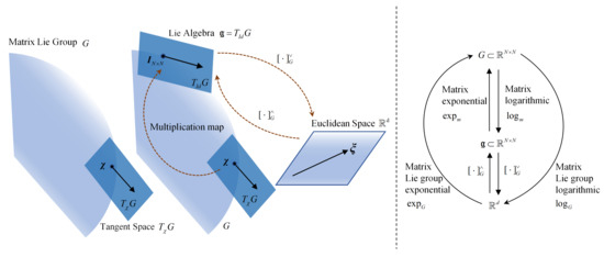
Figure 1.
Schematic of mappings among Lie group, Lie algebra, and Euclidean space. Lie group model is oversimplified. Two distinct identifications of tangent space at with tangent space at afforded by left or right Lie multiplication. Multiplication map includes left and right multiplication.
Lie algebra: Let denote the Lie algebra associated with a d-dimension Lie group; there is . As Lie groups and Lie algebras lack mathematical tools, one needs to identify Lie algebra to Euclidean space for convenient calculation. There is a linear bijection between and , i.e., . This linear bijection is invertible, and its inverse map is defined by . For example, assume vector and Lie algebra ; then, we have and . The middle plot of Figure 1 gives a more intuitive illustration.
Matrix Lie exponential and logarithm maps: Matrix Lie exponential map and its inverse map (the matrix Lie logarithm map) give two bijections between a neighborhood of and a neighborhood of group identity matrix . We define the matrix Lie exponential and logarithm maps as and , respectively, where and are matrix exponential and logarithm operations. Here, matrix exponential and logarithm operations present the link between a Lie group and its unique corresponding Lie algebra: and . For vector , we have . All maps among matrix Lie group G, Lie algebra , and vector space are illustrated in detail on the right plot of Figure 1.
2.2. Uncertainty on Matrix Lie Groups
Most system noise is assumed to be additive white Gaussian noise in Euclidean spaces. However, the approach of additive Gaussian noise is not applicable to Lie groups, as Lie groups lack the addition operation. To describe Gaussian uncertainties for general Lie groups, we adopted the method in [15,16,34], which first assumes the distribution of uncertainty in the Lie algebra to be Gaussian and then maps Gaussian distribution to the corresponding Lie group by exponential mapping.
Consider a d-dimension random variable evolving on G, and let the variable satisfy prior probability distribution . Referring to the definition of the probability distribution for a random variable on a manifold in [15], we give the definition of probability distribution for as follows:
where is a smooth function selected according to the composition of variable that must satisfy , also named “retraction”; is noise-free and represents the mean of random variable ; operator denotes Gaussian distribution in a Euclidean space; is the error covariance matrix associated with uncertainty perturbation ; and is a random Gaussian vector in a Euclidean space. Moreover, distribution is not Gaussian.
The specific operation of function is generally determined by the system’s geometric structure. Left and right Lie group multiplications, and the matrix Lie group exponential are essential parts of no matter the system geometry. Here, with right and left multiplication, we give two simplified definitions of , denoted by and . The components of the variable evolving on G are different, so the expression of function is different in various system dynamics and applications.
3. Bayesian Estimation Based on Bayes–Sard Quadrature Moment Transform
This section aims to find a method to calibrate numerical quadrature errors in the classical sigma point filtering on Lie groups. By taking the cubature Kalman filter into consideration and adopting the BSQMT instead of the cubature transform, we propose a Bayesian estimation method with a generalized measurement model.
3.1. Bayes–Sard Quadrature Moment Transform with Cubature Points
The BSQMT [11] is a universal moment transform proposed to accommodate improper estimation and prediction calibration caused by quadrature error in sigma point filters. The main technique of the BSQMT is the Bayesian quadrature, which treats the numerical process as probabilistic inference, and models the integration error by utilizing stochastic process models. Consider nonlinear vector function
where input is a Gaussian random variable that satisfies Gaussian distribution ; is the output; denotes a known nonlinear transformation function. A brief generalization of the BSQMT algorithm with cubature points is given as follows:
Step 1. Assume that the mean and covariance of random input variable are known. Calculate third-degree cubature points that match the transform moment of random variable
where represents the lower triangular factor in the Cholesky decomposition of ; denotes unit cubature points expressed as
where is the i-th column of identity matrix .
Step 2. Compute the quadrature weight: BSQMT uses a nonzero mean hierarchical Gaussian process (GP) prior model, and Bayes–Sard weights merely depend on the choice of sigma points and basic function space . Let , where is multi-index; then, and . Here, we consider a special base function space in which holds.
Lemma 1.
Let be standard normal distribution, choose cubature points by (4), and construct dimensional function space
Then, a set of quadrature weights can decide the weighted mean of the state variable, and quadrature weights cohere with cubature transform weights .
Proof (Proof of Lemma 1).
See Appendix A. □
With third-degree unit cubature points, quadrature weights are calculated with the following equations:
in which
From Lemma 1, we know that . Thus, we can skip the calculation of in (6).
Step 3. Obtain transformed moments with the following equations:
where . is expected model variance (EMV) of which the value partly depends on the selection of radial basis function (RBF) kernel (covariance of GP model based on unit cubature points) and its parameter. However, in practice, EMV sometimes needs to be reparameterized, but we omitted calculating it here. See [11,38] for the detailed computation of EMV and the selection rules of the basic function.
3.2. Bayesian Estimation on Lie Groups Using BSQMT
In this subsection, we first give a generalized measurement model covering system measurements in two kinds of spaces: Euclidean space and Lie group. Consider random variable and its prior probability density function , follows (1) with known and . Assume that one can establish additional information about the random variable via an observation y:
where is white Gaussian noise with distribution in the vector space, and its dimension depends on the type of ; and represent the observation function, and satisfies the following mapping:
The key to addressing the Bayesian estimation problem is to find parameters and in posterior distribution approximated by . Before estimating , posterior distribution should be found and approximated using BSQMT. Whether the measurement is in a vector space or a Lie group, there is an achievable way to calculate posterior estimate in the vector space and then map it to the Lie group. Hence, while an available measurement exists in a Lie group, we need to transform the matrix Lie group measurement into the vector space by utilizing the inverse mapping of . Inverse map is defined as
In terms of left and right multiplications in both and , if exists in a Lie group, there are actually four possible expansions to map it to the vector space. For instance, similar to [16], suppose measurement function , if ,
else if , there is
where is the joint operator of a Lie group, there is .
In addition, when an available measurement is in a vector space, it fulfils the following equation:
From (14)–(16), we can detect that the optimized measurement function is related to , and . So, giving a novel measurement equation for the derivation of the generalized nonlinear filtering:
where is the new observation, and is the new generalized measurement function.
By using BSQMT, propagated measurement cubature points and the measurement mean are computed:
where is cubature points; and is the mean weight defined in the above subsection. Afterwards, by calculating measurement error covariance and cross-covariance , we obtain gain matrix K and parameters in the approximation of posterior distribution
For converting posterior distribution into a distribution on the Lie group, we reviewed analyses and results in [15,16] and obtained
Lastly, the entire Bayesian estimation procedure is summarized in Algorithm 1.
| Algorithm 1 Bayesian estimation on Lie groups using BSQMT. |
|
4. Proposed Filtering Algorithm
This section presents a Bayes–Sard cubature Kalman filter on matrix Lie groups built on numerical integration error calibration with BSQMT to correct the filtering accuracy and named BSCKF-LG. The proposed BSCKF-LG has two versions: one version uses left multiplication to define “retraction” as left BSCKF-LG; the other uses right multiplication defined as right BSCKF-LG. A systemic method that leverages the maximum likelihood criterion is also proposed to estimate the EMVs. By reconstructing the covariances of the prior state error and the innovation with the innovation sequence in a sliding window, the proposed method estimates EMVs and feeds them back into improved filtering to adjust the Lie Kalman gain matrix.
4.1. Improved Cubature Kalman Filtering on Lie Groups with BSQMT
Consider discrete system dynamics
where k represents the timestamp; is the system state living in a matrix Lie group; and are white Gaussian noise with known covariances in the vector space; and is a known input. According to the above section, we first needed to remodel measurement into , and is in the Euclidean vector space.
The purpose of designing filtering in the Bayesian framework of this model is to approximate posterior distribution . The recursive solution comprises two steps to the proposed filtering problem on Lie groups: propagation and update.
Propagation: start with giving prior probability destiny in the Bayesian framework.
where and are posterior estimation results of the previous moment. Then, try to approximate the state distribution of propagation:
Our work needs to find and . In the above Bayesian estimation, posterior state mean and its associated covariance are estimated using the uncertainty represented by (1). Here, for Model (21), we still used this uncertainty representation and the associated inverse map that has
where stands for error term. The proposed filter first propagates state mean via employing the system’s deterministic part (noiseless state model), that is,
Subsequently, to compute associated covariance , we selected a set of unit cubature points for the BSQMT method and generated sigma points in vector space through . Then, mapping these points to the matrix Lie group and passing the mapped cubature points through noise-free Model (25), we could obtain propagated sigma points . On the basis of this work and with defined inverse map , we obtained prior covariance (see Algorithm 2 for details).
Update: in this procedure, we need to approximate posterior probability distribution.
when each available measurement arrives. Due to the same measurement model, the Bayesian estimation method in Section 3 was applied to compute the posterior state and its associated covariance. The proposed filtering algorithm executes the propagation step and does not perform the update step until the measurement arrives. Algorithm 2 summarizes the proposed filter in detail.
| Algorithm 2 Bayes–Sard cubature Kalman filter (BSCKF-LG). |
|
Remark 1.
The propagation of state means does not need to utilize the BSQMT(or other moment transformation) because (25) was validated by [16] up to the second order. Instead of generating the sigma points directly by the distribution on the Lie group, all work about generating the corresponding sigma points is first done in the Euclidean space and then mapped to the Lie group.
Remark 2.
The unscented Kalman filters on Lie groups in [15,16,17] generate sigma points for the process noise and calculate the covariance matrix of the deviation due to noise. Unlike these filters, process and measurement noise covariancesandin Algorithm 2 are determined by the specified dynamic equation ofand the remodeled measurement function ofto save computing resources.
Remark 3.
BSQMT rules define all Bayes–Sard weights. Weights only depend on the selection of the sigma points and the basic function. The proposed filter requires two different kernel parameter values to obtain EMV values (see [11] for details) because there are two integrated functions. The kernel parameter’s misspecification affects the BSQMT little, so manual parameter tuning of the EMV is available in practice. In the following section, we give a method to obtain the time-varying value of EMV.
4.2. EMV Estimation
In this subsection, we attempt to develop an adaptive BSCKF-LG with time-varying EMVs. To derive the EMV at each instant k, we first assumed that the prior covariance and the innovation covariance are unknown constants. The innovation vector is denoted as , and we consider the following maximum likelihood function of the rebuild measurements :
where denotes the determinant operator, n represents the sliding window size, and C is the constant term. On the basis of (27), the maximum likelihood estimation of the error covariances of the prior state and the prior measurement is derived by
To solve (28), we need to take the partial derivatives of with respect to estimated prior covariance and estimated innovation covariance , and let them be equal to zero:
Subsequently, the maximum likelihood equations are obtained via Equation (29):
and
where denotes the trace operator; corresponds to the th row, th column of with ; similarly, corresponds to the th row, th column of with .
Therefore, the problem of estimating is actually computing the derivation of the innovation covariance with respect to . As stated above, state errors are mapped from the Lie group into the Euclidean space, and prior state error covariance in the Euclidean space can be expressed as . In this article, and . Using (21) and the formula of in Algorithm 2, we first have
Then, and (33) are expressed by the Taylor series expansion about , the estimation error becomes
in which and represent the second- and high-order moments about is derived from the specified dynamic equation of , and its covariance is . To obtain exact equality, we consider the entire high order of by introducing a diagonal matrix , which can scale the approximation error [39,40]:
Similarly, by substituting (18) in and expanding using the Taylor series about , we have
where is the second- and higher-order moment of is defined by the remodeled measurement formula, and its covariance is . To consider the entire higher order, we also introduce a diagonal matrix [39]:
Hence, prior state error covariance and innovation covariance can be expressed by
Lastly, for linear system models (35) and (37), if the Kalman filtering is steady, converges to a constant matrix; and also become constant matrices [41].
On the basis of the above analysis, we assumed that our filtering process inside the sliding window was in a steady state. Consequently, the approximation of in the sliding window was around constant, and there exists such that are 1 for the row and column, while other elements are zeros. In light of the trace definition, we simplified (32) to
Since was approximately constant in the window, we pre- and postmultiplied both sides of (40) with :
Substituting in (41) and letting , the EMV of the measurement function is described as
Next, similar steps were employed to estimate the EMV of the system function. Equations (29) and (31) show that
where or .
Again, since the filtering process was assumed to be stable in the sliding window, approximations of in the window were almost constant, , such that are 1 for the row and column, while other elements are zeros. Equation (43) was pre- and postmultiplied by and ; then, in terms of the trace definition, we simplified (43) to
In sigma point filters, there exists ; thus, (44) can be transformed into
(45) is satisfied if
From Algorithm 2, we know that
Substituting (47) into (46), there readily is
then
with in the window, the maximum likelihood of prior error covariance could be acquired from
Combining and (50), and letting , the estimated EMV could be described as
Remark 4.
As EMVs must be non-negativeandare diagonal matrices, so only estimating the diagonal elements of the EMV matrix is enough. Diagonal elements need to be non-negative; if some diagonal elements are negative, one should set them to zero.
5. Application to Attitude Estimation
In this section, we apply the proposed method to a simulated attitude estimation system and compare it with various filters presented in the cited literature. Consider a rotation rigid body without translation that contains a triaxial gyroscope offering angular velocity at a sampling frequency, a triaxial accelerometer providing acceleration at sampling frequency, and a triaxial magnetometer measuring magnetic field at sampling frequency. For the spacecraft attitude estimation problem, one can replace accelerometers and magnetometers with sun sensors and magnetometers [23]. The attitude kinematics in terms of the unit quaternion is described by
Let accelerometer and magnetometer outputs be observations; observation equations are expressed by [23,42]
in which is the unit quaternion representing the attitude in the body frame with respect to the navigation frame; denotes gyroscope bias; and are uncorrelated white Gaussian noise; is the gravity vector in the navigation frame; and represents Earth’s magnetic field; and and are sensor noises assumed to be white Gaussian noise. Let , which belongs to matrix Lie group , and with the definition of in Section 2, we define the left and right estimation errors as follows:
Then, retractions corresponding with the above estimation errors are
Numerical Simulations
To evaluate estimation quality, numerical simulations were carried out. In the simulations, we selected the north–east–down frame as the navigation frame. The attitude trajectory that lasted 200 s was generated by . The true trajectory without noise and bias is shown in Figure 2. Gyroscope bias was , and gyroscope noise was white Gaussian noise subjected to . Two known corresponding measurement vectors in the navigation frame are and , where is the gravitational acceleration. The noises of the accelerometer and the magnetometer are white Gaussian noise and follow and , respectively. Some sensor parameters are provided by [42]. For filtering, we set the initial covariance matrix as and the initial gyroscope bias as . The kernel scale and kernel length that constituted the kernel parameters were selected to be and .
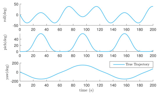
Figure 2.
True trajectory of Euler angles in Cases 1 and 2.
Three cases were considered in our simulations, and in the first two cases, we utilized the trajectory defined above but with different sets of initial attitudes. Case 1 randomly selected the initial attitude from uniform distribution between and , and Case 2 randomly chose the initial attitude from uniform distribution . In Case 3, we used the angular velocity set above, but while 50 s 60 s, angular velocity was set to be ; while 100 s 108 s, angular velocity was set to be ; while 150 s 152 s, angular velocity was set to be . Initial attitudes of Case 3 were the same as those in Case 1.
For each case, we conducted 100 independent Monto Carlo simulations and utilized the following root-mean-square error (RMSE) and averaged RMSE of the Euler angles (roll, pitch, yaw) to evaluate estimation quality:
where M is the total number of simulations; K is the simulation time step; and represent the truth Euler angles(simulated) and the estimated Euler angles, respectively.
With the simulated system and the initial conditions above, we compared nine different filters on Monte Carlo simulations:
- *
- -based CKF ( CKF) that considers the attitude embedded in a special orthogonal group () and the gyroscope bias in a vector space;
- *
- right invariant extended Kalman filter (Right-IEKF) and left invariant extended Kalman filter (Left-IEKF) in [21,23], where the gyroscope bias was treated as part of the Lie group structure;
- *
- right and left cubature Kalman filters on Lie groups (Right-CKF-LG and Left-CKF-LG) [36], which can be treated as extensions of UKF-LG in [16];
- *
- Bayes–Sard quadrature cubature Kalman filter ( BSCKF) derived from [11] by utilizing the same Lie group action as the CKF;
- *
- our proposed right and left BSCKFs on Lie groups (Right-BSCKF-LG and Left-BSCKF-LG) in Section 4;
- *
- the proposed adaptive right BSCKF-LG with time-varying EMVs (Right-BSCKF-LG-adaptive).
We set the sliding window size in both the propagation and update steps of the Right-BSCKF-LG-adaptive to be in Cases 1 and 2, and in Case 3.
Simulation results of Case 1 are illustrated in Figure 3 and Table 1. Figure 3 compares the RMSEs of the Euler angles, while Table 1 summarizes the corresponding ARMSEs. With small initial attitude errors, the proposed BSCKF-type filters with cubature points performed better than other filters did and needed less time to reach a steady state. Right-BSCKF-LG and its adaptive version obviously outperformed the other filters. Simulation results also verified that the performance of Right-IEKF and Right-CKF-LG was similar and slightly better than that of Left-IEKF and Left-CKF-LG under small initial estimation errors. The selection of sliding window size could affect the estimation accuracy of Right-BSCKF-LG-adaptive, and the filtering accuracy of Right-BSCKF-LG-adaptive was not significantly better than that of Right-BSCKF-LG.
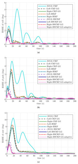
Figure 3.
RMSEs of Euler angles in Case 1. (a) RMSEs of roll angle; (b) RMSEs of pitch angle; (c) RMSEs of yaw angle.

Table 1.
ARMSEs of Euler angles in Case 1.
Case 2 estimation results under large initial attitude errors are demonstrated in Figure 4 and Table 2. These graphs show that the estimation quality of CKF, Left-CKF-LG, and Left-IEKF was poor, especially that of CKF. In contrast, Right-CKF-LG and Right-IEKF achieved better accuracy and robustness than those of Left-CKF-LG and Left-IEKF. Again, BSCKF-type filters performed better. The estimation accuracy of Right-BSCKF-LG and Right-BSCKF-LG-adaptive was better than that of the other filters. Moreover, the accuracy of Right-BSCKF-LG-adaptive improved compared with that of Right-BSCKF-LG. Right-BSCKF-LG-adaptive performed best in the yaw angle and achieved the fastest convergence rate. As seen from the above analyses, the right estimation errors on Lie group are more suitable for attitude estimation with vector measurements.
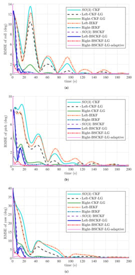
Figure 4.
RMSEs of Euler angles in Case 2. (a) RMSEs of roll angle; (b) RMSEs of pitch angle; (c) RMSEs of yaw angle.

Table 2.
ARMSEs of Euler angles in Case 2.
In Case 3, we assumed that some fast motion occurred in the system trajectory. The true trajectory of Case 3 is shown in Figure 5. Estimation results under small initial attitude errors are indicated in Figure 6 and Table 3. Figure 6 shows that the performance of all filters was worse compared to that in Case 1, partly because of the definition domains of Euler angles. However, the right and left BSCKF-LGs proposed in this paper were still outperformed among all filters, especially adaptive right BSCKF-LG. Table 3 summarizes the ARMSEs of Euler angles. Left BSCKF-LG was slightly more accurate than right BSCKF-LG in this case. The accuracy of Right-BSCKF-LG-adaptive was also greatly improved compared with that of Right-BSCKF-LG.
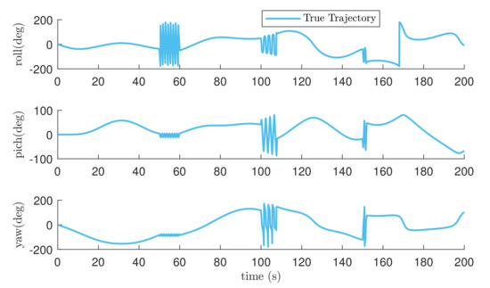
Figure 5.
True trajectory of Euler angles in Case 3.
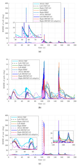
Figure 6.
RMSEs of Euler angles in Case 3. (a) RMSEs of roll angle; (b) RMSEs of pitch angle; (c) RMSEs of yaw angle.

Table 3.
ARMSEs of Euler angles in Case 3.
Figure 7 exhibits the computation times of the compared filters. CKF-LGs and BSCKF-LGs spent more computation time, while IEKFs spent minimal time. When the Bayes–Sard weights were calculated in advance according to the known system-state and measurement dimensions, the computation costs of BSCKF-LGs are almost equal to those of CKF-LGs. Right-BSCKF-LG-adaptive did not significantly increase the computational burden compared with Right-BSCKF-LG. Overall, BSCKF-LGs showed more accurate and robust estimation results in this attitude estimation example.
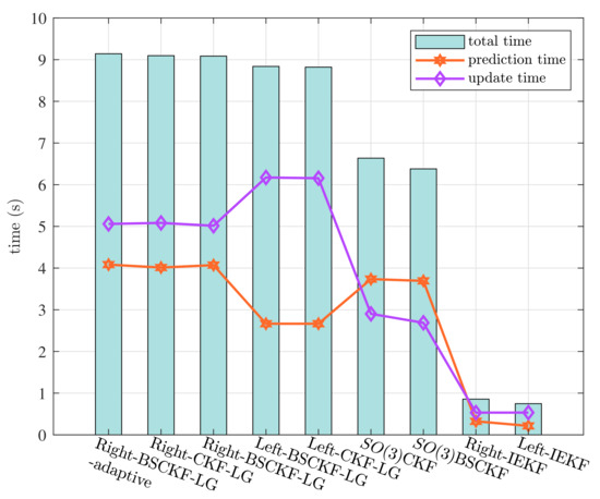
Figure 7.
Execution times of different filters.
6. Conclusions
This article proposed a generalized Bayesian estimation algorithm on matrix Lie groups to calibrate numerical integration errors in classical sigma point filters on Lie groups using BSQMT theory. This Bayesian estimation is applicable to both measurements in Euclidean space and those evolving on the Lie group. Afterwards, with the proposed Lie group Bayesian estimator, we presented a Bayes–Sard cubature Kalman filter on Lie groups that comes in two variants. To obtain more accurate estimation, we then developed an approach to calculate adaptive EMVs. Numerical simulation results on quaternion attitude estimation indicated the superiority of our proposed filters over CKFs on Lie groups and unvariant EKFs. Future work includes exploring novel suitable methods to compute adaptive EMVs and applying the proposed filtering algorithm to visual–inertial navigation and fast drone navigation.
Author Contributions
Conceptualization, H.G.; methodology, H.G.; software, H.G.; validation, H.G., H.L. and X.H.; formal analysis, H.G. and Y.Z.; investigation, H.G., X.H. and H.L.; resources, H.L., X.H. and Y.Z.; data curation, H.G. and Y.Z.; writing—original draft preparation, H.G.; writing—review and editing, H.G. and X.H.; visualization, H.G. and Y.Z.; supervision, H.L.; project administration, H.G.; funding acquisition, H.L. All authors have read and agreed to the published version of the manuscript.
Funding
This research was funded by National Natural Science Foundation of China under Grant 62073265.
Institutional Review Board Statement
Not applicable.
Informed Consent Statement
Not applicable.
Data Availability Statement
The data presented in this study are available on request from the corresponding author. The data are not publicly available because it also forms part of ongoing studies.
Conflicts of Interest
The authors declare no conflict of interest.
Appendix A. Proof of Lemma 1
Because the dimension of the base function space was , weights were the unique solver of linear function . Hence, under the cubature rule:
where . For standard normal distribution, let ; then,
According to the definition of cubature points, it can be inferred from the above formulas that . Thus, we obtain Bayes–Sard weights equal to third-degree cubature transform weights.
References
- Aligia, D.A.; Roccia, B.A.; Angelo, C.; Magallán, G.; Gonzalez, G.N. An orientation estimation strategy for low cost IMU using a nonlinear Luenberger observer. Measurement 2020, 173, 108664. [Google Scholar] [CrossRef]
- Reina, G.; Messina, A. Vehicle dynamics estimation via augmented extended Kalman filtering. Measurement 2018, 133, 383–395. [Google Scholar] [CrossRef]
- Huang, Y.; Zhang, Y.; Bo, X.; Wu, Z.; Chambers, J. A new outlier-robust student’s t based Gaussian approximate filter for cooperative localization. IEEE/ASME Trans. Mechatron. 2017, 22, 2380–2386. [Google Scholar] [CrossRef] [Green Version]
- Kalman, R. A new approach to linear filtering and prediction problems. J. Basic Eng. 1960, 82, 35–45. [Google Scholar] [CrossRef] [Green Version]
- Sunahara Y, Y.K. An approximate method of state estimation for non-linear dynamical systems with state-dependent noise. Int. J. Control 1970, 11, 957–972. [Google Scholar] [CrossRef]
- Julier, S.; Uhlmann, J.; Durrant-Whyte, H.F. A new method for the nonlinear transformation of means and covariances in filters and estimators. IEEE Trans. Autom. Control 2001, 45, 477–482. [Google Scholar] [CrossRef] [Green Version]
- Arasaratnam, I.; Haykin, S.; Elliott, R.J. Discrete-time nonlinear filtering algorithms using Gauss–Hermite quadrature. Proc. IEEE 2007, 95, 953–977. [Google Scholar] [CrossRef]
- Arasaratnam, I.; Haykin, S.; Hurd, T.R. Cubature Kalman filtering for continuous-discrete systems: Theory and simulations. IEEE Trans. Signal Process. 2010, 58, 4977–4993. [Google Scholar] [CrossRef]
- Prüher, J.; Šimandl, M. Bayesian quadrature in nonlinear filtering. In Proceedings of the 12th International Conference on Informatics in Control, Automation and Robotics, Colmar, France, 21–23 July 2015; pp. 380–387. [Google Scholar]
- Pruher, J.; Straka, O. Gaussian process quadrature moment transform. IEEE Trans. Autom. Control 2017, 63, 2844–2854. [Google Scholar] [CrossRef] [Green Version]
- Pruher, J.; Karvonen, T.; Oates, C.J.; Straka, O.; Sarkka, S. Improved calibration of numerical integration error in Sigma-point filters. IEEE Trans. Autom. Control 2020, 66, 1286–1296. [Google Scholar] [CrossRef]
- Bourmaud, G.; Mégret, R.; Giremus, A.; Berthoumieu, Y. From intrinsic optimization to iterated extended Kalman filtering on Lie groups. J. Math. Imaging Vis. 2016, 55, 284–303. [Google Scholar] [CrossRef] [Green Version]
- Hauberg, S.; Lauze, F.; Pedersen, K.S. Unscented Kalman filtering on Riemannian manifolds. J. Math. Imaging Vis. 2013, 46, 103–120. [Google Scholar] [CrossRef]
- Menegaz, H.; Ishihara, J.Y.; Kussaba, H. Unscented Kalman filters for Riemannian state-space systems. IEEE Trans. Autom. Control 2019, 64, 1487–1502. [Google Scholar] [CrossRef] [Green Version]
- Brossard, M.; Barrau, A.; Bonnabel, S. A code for unscented Kalman filtering on Manifolds (UKF-M). In Proceedings of the 2020 IEEE International Conference on Robotics and Automation (ICRA), Paris, France, 31 May–31 August 2020; pp. 1487–1502. [Google Scholar]
- Brossard, M.; Condomines, J.P. Unscented Kalman filtering on Lie groups. In Proceedings of the 2017 IEEE/RSJ International Conference on Intelligent Robots and Systems (IROS), Vancouver, BC, Canada, 24–28 September 2017; pp. 2485–2491. [Google Scholar]
- Brossard, M.; Bonnabel, S.; Barrau, A. Unscented Kalman filter on Lie groups for visual inertial odometry. In Proceedings of the 2018 IEEE/RSJ International Conference on Intelligent Robots and Systems (IROS), Madrid, Spain, 1–5 October 2018; pp. 649–655. [Google Scholar]
- Bonnabel, S. Left-invariant extended Kalman filter and attitude estimation. In Proceedings of the 46th IEEE Conference on Decision and Control, New Orleans, LA, USA, 12–14 December 2007; pp. 1027–1032. [Google Scholar]
- Bonnabel, S.; Martin, P.; Salaun, E. Invariant extended Kalman filter: Theory and application to a velocity-aided attitude estimation problem. In Proceedings of the 48h IEEE Conference on Decision and Control (CDC) Held Jointly with 28th Chinese Control Conference, Shanghai, China, 15–18 December 2009; pp. 1297–1304. [Google Scholar]
- Barrau, A.; Bonnabel, S. Intrinsic filtering on Lie groups with applications to attitude estimation. IEEE Trans. Autom. Control 2015, 60, 436–449. [Google Scholar] [CrossRef]
- Barrau, A.; Bonnabel, S. The invariant extended Kalman filter as a stable observer. IEEE Trans. Autom. Control 2017, 62, 1797–1812. [Google Scholar] [CrossRef] [Green Version]
- Barrau, A.; Bonnabel, S. Invariant Kalman filtering. Annu. Rev. Control Robot. Auton. Syst. 2018, 1, 237–257. [Google Scholar] [CrossRef]
- Gui, H.; de Ruiter, A.H.J. Quaternion invariant extended Kalman filtering for spacecraft attitude estimation. J. Guid. Control Dyn. 2018, 41, 863–878. [Google Scholar] [CrossRef]
- Condomines, J.P.; Hattenberger, G. Nonlinear state estimation using an invariant unscented Kalman filter. In Proceedings of the AIAA Guidance, Navigation, and Control, Boston, MA, USA, 19–22 August 2013; p. 4869. [Google Scholar]
- Condomines, J.P.; Seren, C.; Hattenberger, G. Invariant unscented Kalman filter with application to attitude estimation. In Proceedings of the IEEE 56th Annual Conference on Decision and Control (CDC), Melbourne, VIC, Australia, 12–15 December 2017; pp. 2783–2788. [Google Scholar]
- Condomines, J.P.; Hattenberger, G. Invariant Unscented Kalman Filtering: A Parametric Formulation Study for Attitude Estimation. 2019. hal-02072456. Available online: https://hal-enac.archives-ouvertes.fr/hal-02072456 (accessed on 4 April 2022).
- Barrau, A.; Bonnabel, S. Three examples of the stability properties of the invariant extended Kalman filter. IFAC-PapersOnLine 2017, 50, 431–437. [Google Scholar] [CrossRef]
- Barrau, A.; Bonnabel, S. An EKF-SLAM algorithm with consistency properties. arXiv 2015, arXiv:1510.06263. [Google Scholar]
- Bourmaud, G.; Mégret, R.; Giremus, A.; Berthoumieu, Y. Discrete extended Kalman filter on lie groups. In Proceedings of the 21st European Signal Processing Conference, Marrakech, Morocco, 9–13 September 2013; pp. 1–5. [Google Scholar]
- Bourmaud, G.; Mégret, R.; Arnaudon, M.; Giremus, A. Continuous-Discrete extended Kalman filter on matrix Lie groups using concentrated Gaussian distributions. J. Math. Imaging Vis. 2015, 51, 209–228. [Google Scholar] [CrossRef] [Green Version]
- Phogat, K.S.; Chang, D.E. Invariant extended Kalman filter on matrix Lie groups. Automatica 2020, 114, 108812. [Google Scholar] [CrossRef] [Green Version]
- Phogat, K.S.; Chang, D.E. Discrete-time invariant extended Kalman filter on matrix Lie groups. Int. J. Robust Nonlinear Control 2020, 30, 4449–4462. [Google Scholar] [CrossRef]
- Teng, Z.; Wu, K.; Su, D.; Huang, S.; Dissanayake, G. An Invariant-EKF VINS algorithm for improving consistency. In Proceedings of the 2017 IEEE/RSJ International Conference on Intelligent Robots and Systems (IROS), Vancouver, BC, Canada, 24–28 September 2017; pp. 1578–1585. [Google Scholar]
- Brossard, M.; Bonnabel, S.; Barrau, A. Invariant Kalman filtering for visual inertial SLAM. In Proceedings of the International Conference on Information Fusion, Cambridge, UK, 10–13 July 2018; pp. 2021–2028. [Google Scholar]
- Sjberg, A.M.; Egeland, O. Lie Algebraic unscented Kalman filter for pose estimation. IEEE Trans. Autom. Control 2022, in press. [Google Scholar] [CrossRef]
- Guo, H.; Liu, H.; Zhou, Y.; Li, J. Quaternion invariant cubature Kalman filtering for attitude estimation. In Proceedings of the 2020 3rd World Conference on Mechanical Engineering and Intelligent Manufacturing (WCMEIM), Shanghai, China, 4–6 December 2020; pp. 67–72. [Google Scholar]
- Barrau, A.; Bonnabel, S. Stochastic observers on Lie groups: A tutorial. In Proceedings of the 2018 IEEE Conference on Decision and Control (CDC), Miami, FL, USA, 17–19 December 2018; pp. 1264–1269. [Google Scholar]
- Karvonen, T.; Oates, C.J.; Srkk, S. A Bayes-Sard cubature method. arXiv 2018, arXiv:1804.03016. [Google Scholar]
- Xiong, K.; Liu, L.; Zhang, H. Modified unscented Kalman filtering and its application in autonomous satellite navigation. Aerosp. Sci. Technol. 2009, 13, 238–246. [Google Scholar] [CrossRef]
- Hu, G.; Gao, B.; Zhong, Y.; Gu, C. Unscented kalman filter with process noise covariance estimation for vehicular ins/gps integration system. Inf. Fusio 2020, 64, 194–204. [Google Scholar] [CrossRef]
- Wang, J.; Li, M. Covariance regulation based invariant Kalman filtering for attitude estimation on matrix Lie groups. IET Control Theory Appl. 2021, 15, 2017–2025. [Google Scholar] [CrossRef]
- Nagy, S.B.; Arne, J.T.; Fossen, T.I.; Ingrid, S. Attitude estimation by multiplicative exogenous Kalman filter. Automatica 2018, 95, 347–355. [Google Scholar]
Publisher’s Note: MDPI stays neutral with regard to jurisdictional claims in published maps and institutional affiliations. |
© 2022 by the authors. Licensee MDPI, Basel, Switzerland. This article is an open access article distributed under the terms and conditions of the Creative Commons Attribution (CC BY) license (https://creativecommons.org/licenses/by/4.0/).