Abstract
An advanced LKS (lane keeping system) for use on curving roads is presented to maintain autonomous vehicle driving within the target lane, without unintentional lane departure. There are the following two main objectives in designing this system: one is performing perfect lane keeping and the other is ensuring the dynamic stability of the vehicle, especially when driving on a curving and low-friction road with time-varying high speed. In this paper, a combined vehicle model, consisting of a lane keeping model and a vehicle lateral dynamic model, is firstly introduced. Then, a novel adaptive-weight predictive controller is used to calculate the desired steering angle and the additional yaw moment which provide coordinated control forlane keeping and dynamic stability control. Meanwhile, a square-root cubature Kalman filter-based vehicle sideslip angle observer, with a strong tracking theory modification (ST-SRCKF), is established to estimate the sideslip angle during the driving process. Finally, HIL (hardware-in-the-loop) tests and field tests are constructed, and the results show the effectiveness of our proposed LKS controller and ST-SRCKF sideslip angle estimation.
1. Introduction
Intelligent transportation systems (ITS) represent a key research area in the automobile industry and transportation industry, which use advanced communication technologies and intelligent control methods to improve driving safety and transportation efficiency [1]. Meanwhile, V2X communication technology and intelligent driving technology are essential in ITS. The authors of [2] propose an advanced mmWave routing method with beam alignment for V2X communication, which shows better QoS performance during communication. An LSTM-GAN-based deep reinforcement learning method is designed in [3], to provide a security mechanism for 5G communication links, and simulation results have validated that the autonomous vehicle can successfully overcome the attacks and secure its dynamic system by using this method. Intelligent driving aims to improve fuel economy, driving comfort, and driving safety, and has become a key research area in both academic fields and industry fields [4,5]. For example, LKA (lane keeping assist), as one of the critical technologies of the ADAS (advanced driving assistant system), shows great performance in avoiding road departure and frontal crashes [6]. The authors of [7] tested LKA in two-lane rural roads with different geometric alignments and sections, characterized by variable maintenance conditions for pavements and markings. In general, LKA is constructed to control the car to track alongside the centerline of the desired lane accurately, under driver–automation cooperation, which is the most effective way to avoid/reduce unintentional lane departures due to the failure of the human driver’s performance (such as inattention, drowsiness, and illness) [8,9,10]. The conflict of driving authority between machine and human drivers is still a challenging issue. In [11], a fictive driver activity parameter was introduced into the road–vehicle system to release such an interaction between the human driver and the automation. To avoid conflict situations, [12] proposed a control strategy, allowing both the human driver and the automation system to take actions with the steering wheel, simultaneously and appropriately. The shared control system, consisting of a driver model and a decision-making algorithm, was designed to complete appropriate driving authority transfer, without generating bad interference [13]. Interestingly, there is no need to consider this conflict when designing LKS for autonomous vehicles, due to there being no driver operation [14].
Meanwhile, dynamic stability issues occur when an autonomous vehicle is driving at high speed on a curving road, which must be considered when designing an LKS controller. Thus, a novel high-speed LKS, with dynamic stability control, is proposed in this paper, which not only ensures perfect lane keeping performance, but also maintains lateral dynamic stability. For ensuring lateral dynamic stability, DYC (direct yaw-moment control), as a key function of ESC (electronic stability control), is a general method [15]. Some researchers have applied DYC to ensure driving safety when a vehicle loses dynamic stability. An integrated system, consisting of AFS (active front-wheel steering) and DYC, was designed to control the vehicle yaw rate and the sideslip angle by using a model-matching controller in [16]. A multiple-objective ACC (adaptive cruise control system), combined with DYC, was presented to maintain the lateral dynamic stability and increase the ride comfort under the premise of car-following performance [17]. Meanwhile, the lateral motion and stability of 4WID-EVs were ensured by combining electric power steering systems with DYC [18]. However, DYC may damage lane keeping performance without cooperation with the LKS. Thus, lane keeping systems must be designed through coordination with dynamic stability control, to ensure both lane keeping performance and dynamic stability.
Moreover, understanding how to estimate the vehicle sideslip angle accurately is essential for vehicle dynamic stability control. It is impossible to measure it directly for an autonomous vehicle, due to the large size and high price of the sensor. Some sideslip angle estimation strategies have been proposed in other literature. For example, a sideslip angle estimation algorithm, based on the data fusion of GPS and INS, was designed to improve the estimation accuracy in [19], but it relied on the longitudinal and lateral velocities calculated by the KF method, which is not robust against parameter variations (e.g., changes in tire, road and driving conditions). In addition, a new variable-structure EKF observer, integrated with the sideslip angle rate feedback algorithm, was established in [20], to estimate the vehicle sideslip angle on a low-friction road. However, the EKF could only ensure first-order accuracy, due to the linearization method, and the error could be large when a vehicle is running in a state of instability. In order to construct a more robust and accurate sideslip angle observer, the square-root cubature Kalman filter, with a strong tracking theory modified method (ST-SRCKF), is introduced to estimate the sideslip angle based on a nonlinear vehicle dynamic model.
The overall architecture of the proposed LKS is presented in Figure 1, which mainly includes the following three modules: the sensor and estimator, and the upper controller and the lower controller. Meanwhile, we focused on how to construct the control strategy of LKS and sideslip angle estimation; how to identify lane line and estimate road friction coefficients in the sensor and estimator module will not be key points in this paper. Algorithm 1 shows the brief processing steps of the proposed LKS controller. According to the overall process, the remainder of this paper is organized as follows: Section 2 presents the vehicle lateral dynamic model and the vehicle lane keeping model. Section 3 introduces the design of the high-speed curving LKS, based on an adaptive-weight predictive controller, in detail. How to establish an ST-SRCKF sideslip angle estimator is shown in Section 4. The performance of the proposed LKS and sideslip angle estimator is verified by HIL tests and a field test in Section 5. The conclusion is drawn in Section 6.
| Algorithm 1: The brief processing of proposed LKS controller |
| Proposed LKS controller Input: Output: |
| Step 1: Construct vehicle dynamic model and lane keeping model |
Step 2: Design upper controller
Step 5: Results estimation |
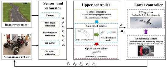
Figure 1.
Overall structure of proposed LKS.
2. Related Models
2.1. Vehicle Dynamic Model
In order to ensure the accuracy of estimating the vehicle sideslip angle, a four-wheeled vehicle model is introduced, as shown in Figure 2. The longitudinal, lateral, and yaw motion functions are shown as follows:
where m is the vehicle mass; are the lateral forces of the front left wheel, front right wheel, rear left wheel and rear right wheel, respectively; are the longitudinal forces. represent the distance from the center of mass to the front and rear axles, respectively, is the wheel base, is the steering angle, and is the inertia moment about the vehicle vertical axle.
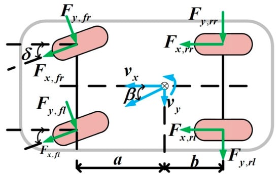
Figure 2.
Four-wheeled vehicle dynamics.
Meanwhile, in order to calculate the tire forces of each wheel in nonlinear regions, the MF (magic formula) tire model [21] is used in this paper, as follows:
If represents the lateral tire force, should be set as the wheel sideslip angle . Moreover, if represents the longitudinal force, is set as the longitudinal slip ratio , which can be calculated as follows:
is the longitudinal velocity of each wheel and is the wheel velocity. The longitudinal force is calculated as follows:
The lateral force is calculated as follows:
The factors and can be determined by tire force tests.
The four-wheeled vehicle dynamic model is mainly used to estimate the vehicle sideslip angle. Its nonlinearity and high calculation burden lead to great difficulty in online optimization for dynamic stability control. Thus, a 2DOF dynamic model (as shown in Figure 3) is established, which has been extensively used for vehicle dynamic control [18,21,22,23].
where and are the cornering stiffness of the front and rear wheels, respectively, and represents the additional yaw moment.

Figure 3.
2DOF vehicle dynamic model.
2.2. Lane Keeping Model
Figure 4 shows the lane keeping model, which reveals the geometric relationship between the centerline of the target lane and the autonomous vehicle. is the heading offset, which is shaped by the tangential direction of the required lane centerline and the vehicle’s heading at a previewed distance . presents the lateral deviation, which is the distance from the current vehicle position to the required lane at the previewed point. is the curvature of the required lane centerline. The lane keeping model can be calculated as follows [24,25,26]:
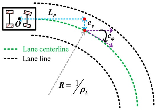
Figure 4.
Lane keeping model.
3. The Design of the Proposed LKS
When an autonomous vehicle runs on a curving road at time-varying high speed, the vehicle may lose lateral dynamic stability because of inadequate tire lateral force. Thus, the lane keeping performance and the lateral dynamic stability must be considered at the same time in the process of designing the LKS. Based on the above description and discussion, an advanced LKS integrated with dynamic control is proposed, which has a hierarchical control architecture, consisting of an upper controller and a lower controller. An adaptive predictive control-based upper controller calculates the desired steering angle and additional yaw moment by minimizing the cost function, subject to certain I/O constraints. The lower controller converts the desired steering angle and yaw moment into the corresponding driving torque of the steering motor and different brake pressures of the four wheels.
3.1. Upper Controller
In order to solve multi-objective optimization tasks using a predictive framework, a combined model should be established first. Combined with Equations (10)–(13), a four-state space model can be obtained, as shown in Equations (14) and (15). is the state vector, , denotes the external disturbance, which is defined as , represents the control input, , and is the control output, .
where
In order to reduce, or even eliminate, the static error, an incremental model is obtained from Equation (14). Meanwhile, a discrete model can be calculated by adopting a Euler algorithm in Equation (14), with the sampling frequency . Then, a discrete, incremental form of control model can be established as follows [27]:
where
Based on Equation (15), the control output can be transformed into an incremental form as follows:
In order to derive the predictive equation of the control system, we make the following assumptions: (1) beyond the control horizon , the control variables will remain unchanged, i.e., . The external disturbance remains constant after time k, i.e., . Based on the assumptions mentioned above, we can deduce the following predictive equations of the stated increments:
The -step prediction output vector and -step input vector can be defined as follows:
The prediction output vector can be obtained as shown in Equation (24), as follows:
where
.
The proposed LKS not only ensures perfect lane keeping performance, but also guarantees effective lateral dynamic stability, especially when an autonomous vehicle is driving at high speed on a curving road. Thus, a cost function is defined as follows, to achieve multi-objective optimization:
There are two items on the right side of the cost function. The first is to punish the tracking performance error and dynamic stability error. The second is to punish the change in control input, to ensure ride comfort. represents the control output reference matrix, which is shown in Equation (30), as follows:
In this paper, we set the reference values . and are weighted matrices of the control outputs and increments in the control inputs, respectively, which can be presented in a standard form, as follows:
where
The adaptive-weight method is beneficial for improving the predictive control performance. For example, when a vehicle is running in a state of dynamic instability, larger values of and are meaningful. When running with stability, more accurate lane keeping performance is needed. Thus, an FLC-based (Fuzzy logic control) adaptive-weight method is introduced in this paper. First, we calculate the lane keeping index and the dynamic stability index as follows:
where and are weight coefficients. Two fuzzy control inputs, including the lane keeping index ratio and the dynamic stability index ratio , are defined in Equation (37). All the inputs of the fuzzy controller can be fuzzified into the following three fuzzy sets: ZO (zero), PS (positive small), and PB (positive big). We define the lane keeping weight ratio and dynamic stability weight ratio as fuzzy control outputs (shown in Equation (38)), and the output is fuzzified into the following four fuzzy sets: ZO (zero), PB (positive big), PM (positive medium), PS (positive small).
Further, and are the maximum measurements of the lane keeping index and the dynamic stability index. Additionally, = 10 and are the maximum measurements of lane keeping weight and dynamic stability weight. The membership functions associated with the inputs and outputs of the fuzzy controller are shown in Figure 5.

Figure 5.
Membership functions of inputs and outputs: (a) the membership function of , (b) the membership function of , and (c) the membership function of the outputs.
The Fuzzy rules that consider correlations between the inputs and the outputs are listed in Table 1 and Table 2.

Table 1.
Fuzzy rules of the lane keeping weight ratio.

Table 2.
Fuzzy rules of the dynamic stability weight ratio.
The FLC-based adaptive-weight method calculates and online. Then, the weight values in Equations (34) and (35) can be obtained by calculating the following equations:
We define an auxiliary variable to solve the optimization problem, as follows:
The new form of cost function can be constructed as follows:
where
The multi-objective optimization problem can be transformed as follows:
Considering the extremum condition of Equation (41), we can obtain the following equation:
By solving Equation (44), the extremum can be calculated as in Equation (45). Because the second derivative of is always greater than zero, the solution to Equation (45) is the optimization of the values.
3.2. Lower Controller
The desired steering angle and the additional yaw moment generated from the upper controller are used to ensure the lane keeping performance and to stabilize the vehicle, respectively. The desired steering angle can be realized by controlling the torque of the EPS motor. The additional yaw moment can be applied to the vehicle by exerting differential brake forces on each of the four wheels. According to the Newtonian mechanics formula, we can obtain the following equations:
where represents the acceleration, and are the longitudinal tire forces of the left front wheel, right front wheel, left rear wheel and right rear wheel, respectively. The differential braking strategy is used to calculate the braking pressure of each wheel.
4. ST-SRCKF-Based Sideslip Angle Estimator
The sideslip angle and yaw rate are crucial for vehicle dynamic stability control. The yaw rate can be obtained through a yaw rate sensor fixed on the vehicle. However, it is impossible to measure the sideslip angle directly, due to the expense of the sensor. Thus, an economical and accurate sideslip angle observer is established, based on ST-SRCKF, in this section. First, a suboptimal fading factor is introduced to the covariance matrix of state prediction to adjust the gain matrix, which is calculated using a strong tracking theory. Next, an ST-SRCKF sideslip angle observer is established to estimate the sideslip angle.
4.1. Strong Tracking Theory
Based on the four-wheeled vehicle dynamic model (Equations (2) and (3)), a discrete form system model, with a modified Euler method, is established as follows:
where is the estimated system state and denotes the measured state. and are the model noise and measurement noise, which are assumed as gaussian white noise with zero mean and as independent of each other. Moreover, can be calculated as shown in Equation (49), as follows:
The strong tracking theory is described as follows [28]:
In addition, is the fading factor. In order to improve the instantaneity of the algorithms, the suboptimal algorithm is applied to calculate the fading factor [29], as follows:
where denotes the matrix trace, and is the covariance matrix of the real output residual sequence, which can be calculated as follows:
where is the forgetting factor and presents the theoretical output residual sequence.
4.2. ST-SRCKF Estimator
The strong tracking theory is sensitive to measurement noise, which leads to a reduction in tracking accuracy, but it has the ability to obtain the orthogonality of the residual sequence. Meanwhile, SRCKF is robust to measurement noise. Thus, a square-root cubature Kalman filter-based estimator, with a modified strong tracking theory, is established to improve the prediction accuracy and filter stability, which is described in the following section.
4.2.1. Time Update
- The cubature points and propagated cubature points are calculated as follows:where is the cubature point, is the propagated cubature point, and denote the system state dimension, is the basic cubature point, and denotes the point from set .
- 2.
- The predicted state can be calculated as follows:
- 3.
- The square-root coefficient of the prediction error covariance matrix can be calculated as follows:where is the square-root coefficient of , and , means the weight coefficient, presents a general triangularization algorithm [29], and can be described as follows:
- 4.
- The prediction error covariance matrix can be calculated as follows:
4.2.2. Measurement Update
- The cubature points and propagated cubature points can be calculated as follows:
- 2.
- The predicted measurement can be calculated as follows:
- 3.
- The innovation covariance matrix and its square-root coefficient are calculated as follows:where is the square-root coefficient of , with , and the innovation covariance matrix can be described as follows:
- 4.
- The cross-covariance matrix can be calculated as follows:
- 5.
- The fading factor , based on Equations (51)–(53), is calculated.
- 6.
- The prediction error covariance matrix, with the modified fading factor and its square-root coefficient, is calculated as follows:
- 7.
- The modified square-root coefficient of innovation covariance matrix and the cross-covariance matrix are calculated by introducing the modified prediction error covariance matrix to Equations (60)–(65).
- 8.
- The gain matrix and evaluate cross-covariance matrix are calculated as follows:
- 9.
- The square-root coefficient of error covariance matrix is estimated as follows:
5. Results and Discussion
We compared the estimation performance of the ST-SRCKF-based sideslip angle estimator with that of an EKF in a field test, and the results verified the effectiveness of our proposed observer. Meanwhile, HIL tests were carried out to verify the superiority of our proposed LKS controller in lane keeping and vehicle dynamic stability.
5.1. Sideslip Angle Estimation
Figure 6 shows the experimental vehicle. Field tests were performed on the ice-cream road with a friction coefficient of 0.35. During the testing process, the driver controlled the steering wheel angle and velocity by himself (Figure 7 shows the steering wheel angle and Figure 8 presents the vehicle speed). The testing data were used to validate the performance of our proposed ST-SRCKF-based sideslip angle observer, as shown in Figure 9. In a word, our proposed ST-SRCKF observer performs better than an EKF, and it shows strong robustness to estimation divergence under severe conditions. For example, violent steering action and acceleration/deceleration operation were conducted after 10 s, and the real maximum sideslip angle reached −8.816 degree. Our ST-SRCKF estimator obtained –9.238 degree for the maximum sideslip angle, and the estimation error was less than 4.78%, which highlights that the ST-SRCKF observer has great accuracy when estimating the sideslip angle. However, the EKF-based observer only obtained −15.212 degree in estimating the maximum sideslip angle, and the error was more than 38.52%, which verifies that our ST-SRCKF observer performs better than an EKF.
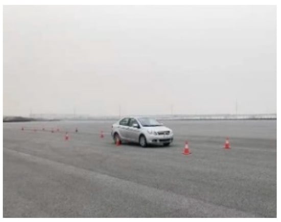
Figure 6.
Testing vehicle.
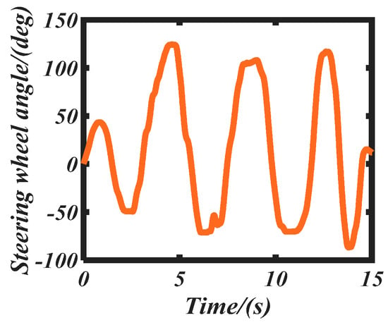
Figure 7.
Steering angle.
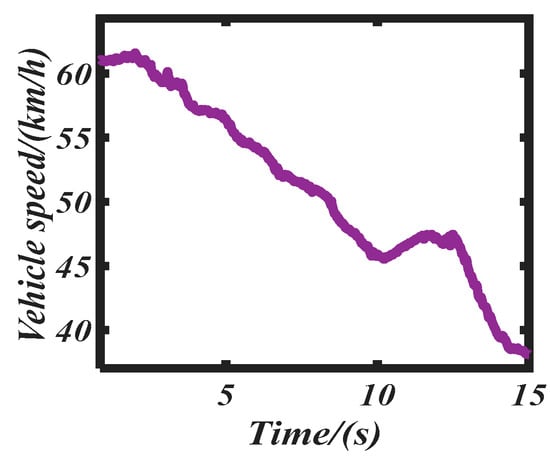
Figure 8.
Vehicle speed.
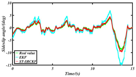
Figure 9.
Real sideslip angle and estimated angle.
5.2. Lane Keeping Performance
For confirming the effectiveness of accurate lane keeping and strong dynamic stability of our proposed LKS, two compared controllers were designed; the first controller was a traditional LKS, without dynamic control. We set the weights to in Equations (33) and (34). The other is a traditional LKS with DYC. A severe testing condition was established, where the speed changed between 80 km/h and 100 km/h. Figure 10 shows a kind of HIL platform, and Table 3 shows the brief road geometry characteristics for high-speed lane keeping testing in Carsim.
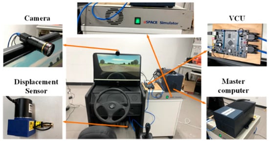
Figure 10.
HIL platform.

Table 3.
Road geometry characteristics.
The testing results are presented in Figure 11, Figure 12, Figure 13, Figure 14, Figure 15, Figure 16 and Figure 17. Figure 11 shows the reference lane centerline and the trajectories controlled by our proposed LKS, a conventional LKS and an LKS + DYC. In Figure 11, the trajectory without DYC deviates from the reference lane at X = 169 m, which means that the vehicle slips seriously. The yaw rate and steering angle are shown in Figure 13 and Figure 15, respectively. However, the trajectory controlled by our proposed controller and the LKS + DYC can track the reference lane accurately. Furthermore, the maximum lateral error from the reference centerline controlled by our proposed controller is less than 0.1 m, and that of the LKS + DYC is 0.318 m. Based on the above analysis, we can observe that the proposed LKS controller has a better lane keeping performance.
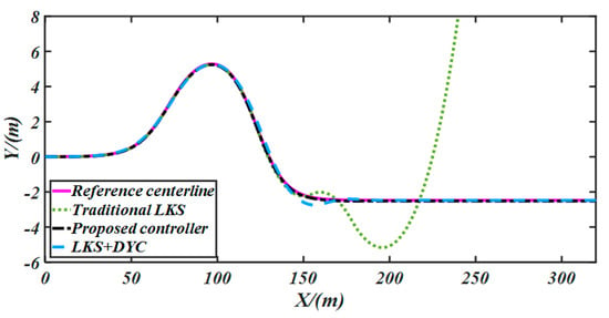
Figure 11.
Trajectories controlled by three controllers.
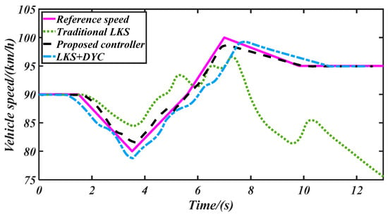
Figure 12.
The nominal vehicle speed and real vehicle speed controlled by different controllers.
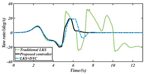
Figure 13.
Vehicle yaw rate controlled by different controllers.
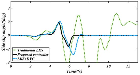
Figure 14.
Vehicle sideslip angle controlled by different controllers.
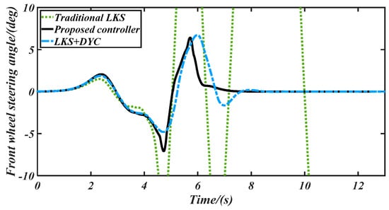
Figure 15.
The front steering angle controlled by different controllers.
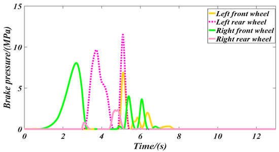
Figure 16.
Brake pressure controlled by our proposed controller.
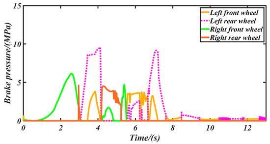
Figure 17.
Brake pressure controlled by conventional LKS + DYC.
The comparison of dynamic stability performance with three controllers is shown in Figure 13 and Figure 14, which present the yaw rate and sideslip angle, respectively. We can conclude, from these figures, that the vehicle with the traditional LKS loses its dynamic stability after 6 s, and the curves of its sideslip angle and yaw rate vibrate sharply. On the contrary, the vehicle dynamic stability is ensured effectively by our proposed controller and the LKS + DYC during the whole lane keeping process. In Figure 13, the maximum yaw rate with our proposed LKS is less than 20 degree/s, but the maximum controlled by the conventional LKS is over 35 degree/s. As shown in Figure 14, the maximum sideslip angle controlled by our proposed controller is less than 2 degree, which means that the vehicle maintains lateral dynamic stability during the steering process with time-varying high speed. However, the sideslip angle by the traditional LKS diverges after 6 s. Moreover, our proposed controller has a better dynamic stability performance than that of the LKS + DYC. For example, at t = 6.9 s, the vehicle controlled by our LKS maintains strong dynamic stability, but a big slip appears to be controlled by the LKS+DYC, due to a contradiction between the lane keeping and dynamic stability controls. More precisely, at t = 6.9 s, the conventional LKS calculates a front steering angle of δ = −1.638 degree to realize accurate lane keeping. Meanwhile, the DYC also applies significant brake pressure to maintain the vehicle stability, as shown in Figure 17. The steering operation and braking operation are contradictory to dynamic stability control without coordination, which leads to slip. However, our proposed LKS can coordinate the steering operation and braking operation accurately, to maintain lane keeping and vehicle dynamic stability.
6. Conclusions
An advanced LKS with sideslip angle estimation is introduced in this paper, designed to keep a vehicle tracking within the desired lane, and maintain dynamic stability. First, the vehicle–road model and the vehicle dynamic model are established. Based on the models mentioned above, the adaptive-weight predictive controller is used to calculate the desired steering angle and the additional yaw moment. Then, an ST-SRCKF sideslip angle estimator is established to observe the sideslip angle accurately during the lane keeping process. Moreover, the upper controller sends the steering signal to the EPS motor through the CAN bus, and the additional yaw moment can be obtained by differential braking, which applies different brake pressures to the four brake wheel cylinders. Finally, field tests and HIL tests were conducted to prove that the proposed LKS controller can not only keep the vehicle driving in the desired lane, without departure, but also perform well at maintaining vehicle dynamic stability with accurate sideslip angle estimation, while driving in a low-friction lane at time-varying speed.
Author Contributions
H.W. focused on conducting experiments and writing the paper. B.L. focused on designing method derivation, and J.Q. helped in conducting the experiment. All authors have read and agreed to the published version of the manuscript.
Funding
This research was funded by Fundamental Research Funds for the Central Universities of China, grant number 2021JBM024.
Institutional Review Board Statement
Not applicable.
Informed Consent Statement
Not applicable.
Data Availability Statement
Not applicable.
Conflicts of Interest
It should be understood that none of the authors have any financial or scientific conflicts of interest with regard to the research described in this manuscript.
References
- Ou, D.; Liu, R.; Rasheed, L.; Shi, L.; Li, H. Operation performance of tram lanes with intermittent priority with the coexistence of regular and automatic vehicles. J. Intell. Transp. Syst. 2021, 1–12. [Google Scholar] [CrossRef]
- Rasheed, L.; Hu, F.; Zhang, L. Deep reinforcement learning approach for autonomous vehicle systems for maintaining security and safety using LSTM-GAN. Veh. Commun. 2020, 26, 100266. [Google Scholar] [CrossRef]
- Rasheed, L.; Hu, F.; Hong, Y.; Balasubramanian, B. Intelligent Vehicle Network Routing with Adaptive 3D Beam Alignment for mmWave 5G-Based V2X Communications. IEEE Trans. Intell. Transp. Syst. 2021, 5, 2706–2718. [Google Scholar] [CrossRef]
- Wang, H.; Liu, B.; Ping, X.; An, Q. Path Tracking Control for Autonomous Vehicles Based on an Improved MPC. IEEE Access 2019, 7, 161064–161073. [Google Scholar] [CrossRef]
- Lu, S.; Cen, S.; Hu, X. Integrated Control of Braking and Steering Subsystems for Autonomous Vehicle based on an Efficient Yaw Moment Distribution. IEEE Trans. Ind. Electron. 2017. [Google Scholar] [CrossRef]
- Pappalardo, G.; Cafiso, S.; Graziano, A.; Severino, A. Decision Tree Method to Analyze the Performance of Lane Support Systems. Sustainability 2021, 13, 846. [Google Scholar] [CrossRef]
- Cafiso, S.; Pappalardo, G. Safety effectiveness and performance of lane support systems for driving assistance and automation—Experimental test and logistic regression for rare events. Accid. Anal. Prev. 2020, 148, 105791. [Google Scholar] [CrossRef]
- Yan, F.; Wang, K.; Zou, B. LiDAR-based Multi-Task Road Perception Network for Autonomous Vehicles. IEEE Access 2020, 8, 86753–86764. [Google Scholar] [CrossRef]
- Fahmy, H.; Ghany, M.; Baumann, G. Vehicle Risk Assessment and Control for Lane-Keeping and Collision Avoidance at Low-Speed and High-Speed Scenarios. IEEE Trans. Veh. Technol. 2018, 67, 4806–4818. [Google Scholar] [CrossRef]
- Ji, J.; Khajepour, A.; Melek, W.; Huang, Y. Path Planning and Tracking for Vehicle Collision Avoidance Based on Model Predictive Control with Multiconstraints. IEEE Trans. Veh. Technol. 2017, 66, 952–964. [Google Scholar] [CrossRef]
- Nguyen, A.; Sentouh, C.; Popieul, J. Driver-automation cooperative approach for shared steering control under multiple system constraints: Design and experiments. IEEE Trans. Ind. Electron. 2017, 64, 3819–3830. [Google Scholar] [CrossRef]
- Saleh, L.; Chevrel, P.; Claveau, F.; Lafay, J.; Mars, F. Shared steering control between a driver and an automation: Stability in the presence of driver behavior uncertainty. IEEE Trans. Intell. Transp. Syst. 2013, 14, 974–983. [Google Scholar] [CrossRef]
- Sentouh, C.; Soualmi, B.; Popieul, J.; Debernard, S. Cooperative steering assist control system. In Proceedings of the IEEE International Conference on Systems, Man and Cybernetics, Manchester, UK, 13–16 October 2013. [Google Scholar]
- Parr, G.; Hailes, S.; How, J.; McGeehan, J.; Guo, Y. Guest Editorial: Communications Challenges and Dynamics for Unmanned Autonomous Vehicles. IEEE J. Sel. Area. Commun. 2012, 30, 849–851. [Google Scholar] [CrossRef]
- Li, L.; Jia, G.; Chen, J.; Zhu, H.; Cao, D.; Song, J. A novel vehicle dynamics stability control algorithm based on the hierarchical strategy with constrain of nonlinear tyre forces. Veh. Syst. Dyn. 2015, 53, 1093–1116. [Google Scholar] [CrossRef]
- Nagai, M.; Shino, M.; Gao, F. Study on integrated control of active front steer angle and direct yaw moment. JSAE Rev. 2002, 23, 309–315. [Google Scholar] [CrossRef]
- Cheng, S.; Li, L.; Mei, M.; Nie, Y.; Zhao, L. Multiple-Objective Adaptive Cruise Control System Integrated with DYC. IEEE Trans. Veh. Technol. 2019, 68, 4550–4559. [Google Scholar] [CrossRef]
- Shuai, Z.; Zhang, H.; Wang, J.; Li, J.; Ouyang, M. Combined AFS and DYC control of four-wheel-independent-drive electric vehicles over CAN network with time-varying delays. IEEE Trans. Veh. Technol. 2014, 63, 591–601. [Google Scholar] [CrossRef]
- Ni, J.; Hu, J. Dynamics control of autonomous vehicle at driving limits and experiment on an autonomous formula racing car. Mech. Syst. Signal Process. 2017, 90, 154–174. [Google Scholar] [CrossRef]
- Li, L.; Jia, G.; Ran, X.; Song, J.; Wu, K. A variable structure extended Kalman filter for vehicle sideslip angle estimation on a low friction road. Veh. Syst. Dyn. 2014, 52, 280–308. [Google Scholar] [CrossRef]
- Li, L.; Lu, Y.; Wang, R.; Chen, J. A Three-Dimensional Dynamics Control Framework of Vehicle Lateral Stability and Rollover Prevention via Active Braking With MPC. IEEE Trans. Ind. Electron. 2017, 4, 3389–3401. [Google Scholar] [CrossRef]
- Cheng, S.; Li, L.; Guo, H.; Chen, Z.; Song, P. Longitudinal Collision Avoidance and Lateral Stability Adaptive Control System Based on MPC of Autonomous Vehicles. IEEE Trans. Intell. Transp. Syst. 2020, 21, 2376–2385. [Google Scholar] [CrossRef]
- Zhang, H.; Wang, J. Vehicle lateral dynamics control through AFS/DYC and robust gain-scheduling approach. IEEE Trans. Veh. Technol. 2016, 65, 489–494. [Google Scholar] [CrossRef]
- Guo, J.; Luo, Y.; Li, K.; Dai, Y. Coordinated path-following and direct yaw-moment control of autonomous electric vehicles with sideslip angle estimation. Mech. Syst. Signal Process. 2018, 105, 183–199. [Google Scholar] [CrossRef]
- Guo, J.; Li, L.; Li, K.; Wang, R. An adaptive fuzzy-sliding lateral control strategy of automated vehicles based on vision navigation. Veh. Syst. Dyn. 2013, 51, 1502–1517. [Google Scholar] [CrossRef]
- Guo, J.; Hu, P.; Wang, R. Nonlinear coordinated steering and braking control of vision-based autonomous vehicles in emergency obstacle avoidance. IEEE Trans. Intell. Transp. Syst. 2016, 17, 3230–3240. [Google Scholar] [CrossRef]
- Choi, M.; Choi, S. Model predictive control for vehicle yaw stability with practical concerns. IEEE Trans. Veh. Technol. 2014, 63, 3539–3548. [Google Scholar] [CrossRef]
- Jwo, D.; Yang, C.; Chuang, C. Performance enhancement for ultra-tight GPS/INS integration using a fuzzy adaptive strong tracking unscented Kalman filter, Nonlinear Dynamics. Nonlinear Dyn. 2013, 73, 377–395. [Google Scholar] [CrossRef]
- Arasaratnam, I.; Haykin, S. Cubature Kalman filters. IEEE Trans. Autom. Control 2009, 54, 1254–1269. [Google Scholar] [CrossRef] [Green Version]
Publisher’s Note: MDPI stays neutral with regard to jurisdictional claims in published maps and institutional affiliations. |
© 2022 by the authors. Licensee MDPI, Basel, Switzerland. This article is an open access article distributed under the terms and conditions of the Creative Commons Attribution (CC BY) license (https://creativecommons.org/licenses/by/4.0/).