Abstract
As the most important device of an Autonomous Underwater Vehicle (AUV), thrusters are one of the main sources of fault. If the thruster fault can be diagnosed in the early stage, it would give more time to guarantee the safety of an AUV. Fault feature extraction is the premise of fault diagnosis. The traditional feature calculation methods extract fault features from one domain. These methods work well in the case of high fault severity, but poorly in the case of weak fault severity. In addition, for weak faults, the fault features extracted by the traditional methods may not meet the monotonic relationship with fault severity and cannot be used in fault severity identification. Aiming at these problems, through experimental data analysis, this paper excludes the features that do not meet the law from the 52 selectable fault features in the time domain, frequency domain and time-frequency domain. Aiming at the problem that there is no useful feature in the frequency domain, a new feature calculation method is proposed, and the order of magnitude of the available feature is given, which provides concise and accurate information for subsequent fault feature fusion and fault severity identification.
1. Introduction
At present, the Autonomous Underwater Vehicle (AUV) plays an important role in the detection of marine resources [1]. Safety is one of the vital issues for AUV research and application during unmanned and cableless operations in the marine environment [2]. Fault diagnosis technology is a key technology to ensure its safety [2]. As the component with the heaviest load and the highest use frequency in an AUV, the thruster is one of the main fault sources of an AUV [3]. Fault diagnosis technology of thrusters has important research significance and practical value to improve the safety of AUVs [4].
The thruster fault diagnosis technology of AUVs has attracted the attention of many scholars and its main research focuses on the serious thruster fault (loss of effectiveness > 10%) [5,6,7]. Different from serious thruster faults, most weak thruster faults (loss of effectiveness ≤ 10%) are the faults in the early stage. The weak fault feature of thrusters and external interference overlap in the frequency band, and the AUV closed-loop control system has a certain compensation effect on ocean current interference and even thruster fault [8,9]. All of these increase the difficulty of a weak fault diagnosis of thrusters. Thus, research on weak fault diagnosis technology of thrusters can give more time to guarantee the safety of an AUV, so as to avoid fatal accidents. There is still little literature on weak thruster faults at present [10,11].
The process of weak fault diagnosis of thrusters mainly includes fault feature extraction and fault severity identification [12]. This paper studies the problem of fault feature extraction.
Generally, fault features are extracted in three domains: time domain, frequency domain, or time-frequency domain [13,14], and several features are extracted in one domain [15]. In the past, only one domain was mostly selected to extract several fault features for fault severity identification [16,17,18,19,20]. The existing fault feature extraction methods include wavelet decomposition, empirical mode decomposition, sparse decomposition, and other methods. Liu, et al. [21] proposed an AUV fault diagnosis method based on wavelet decomposition. This method transforms the surge velocity and yaw angle in the time domain into frequency domain features by the wavelet method. After that, the fractal method is used to extract the fractal characteristics of the original signal, approximation coefficient, and detail coefficient to realize the fault diagnosis of the fault severities greater than 10% (10% to 50%). However, when the method handles 5% weak faults, it cannot obtain satisfactory fault feature values. Zhang, et al. [22] proposed an AUV fault extraction method based on empirical modal decomposition (EMD). This method converts the surge velocity and control quantity in the time domain into frequency domain features by EMD and wavelet methods, so as to achieve blind source separation and enhancement of fault features. This method is also difficult to extract the fault feature values of weak fault [23]. In this study, it was found that for the serious thruster faults, most of the features extracted in the three domains could be used for subsequent fault severity identification. However, for the weak thruster faults, among the fault features extracted in the three domains, some of the fault features do not satisfy the law of monotonous increase (or monotonic decrease) with the increase of the fault degree. In addition, although some of the fault features conform to the monotonic law, the difference of fault features between adjacent fault severities is too small to be used for fault severity identification. None of these features can be used for the subsequent fault severity identification. Therefore, for weak fault feature extraction of thrusters, it is necessary to determine the useful fault features and eliminate the useless ones at first.
For AUV fault diagnosis, there are multiple input signals such as surge velocity signal, yaw angle signal, control signal, tracking error (and so on), and each input signal has multiple features in one domain. Moreover, for all the features of all input signals in the three domains, not all features are useful. Therefore, to maximize the extraction of fault features for the weak fault diagnosis of AUVs and provide refined and accurate information for subsequent fault severity identification, fault features should be extracted in different domains (time domain, frequency domain, and time-frequency domain), and the unusable feature should be eliminated. In terms of solving the problem of weak fault feature extraction of thrusters, there is no literature report on which features are useful and which are not. Furthermore, in the experimental study, it was found that the traditional feature calculation method is difficult to extract useful features in a certain domain. Therefore, it is necessary to improve the traditional feature calculation method.
Based on the above analysis, in order to improve the accuracy of subsequent weak fault diagnosis, this paper looks for scientific and reasonable fault characteristics from different domains. The main innovation points of this paper are as follows:
(1) Aiming at the problem of feature extraction of weak thruster fault, based on the experimental data of AUVs with different fault severity, this paper studies the variation trend and characteristics of different features in multiple domains (time domain, frequency domain and time-frequency domain), and determines the scientific and reasonable fault features.
(2) To enlarge the number of useful fault features as much as possible, the features without monotonic change law are improved to show an obvious monotonic change law with the fault severities, and their effectiveness is verified by experiments.
(3) Finally, the useful fault features in time domain, frequency domain, and time-frequency domain are extracted, and the order of magnitude of different fault features is given, which lays a foundation for subsequent fault feature fusion.
This paper is organized as follows: In Section 2, the experimental carrier, experimental environment and thruster fault simulation methods are briefly introduced. In Section 3, the research ideas of this paper are proposed. In Section 4, the fault feature of each domain is briefly described. In Section 5, taking the surge velocity signal as an example, the law of all features in the time domain, frequency domain, and time-frequency domain is analyzed, and aiming at the problem that there are no useful features in the frequency domain, a new calculation method of feature is proposed. In Section 6, for the commonly used AUV signals such as control quantity, yaw angle and tracking error, according to the experimental data, the useful features are extracted, and the order of magnitude of each feature is given, which provides scientific and reasonable features for feature fusion and fault degree identification. Finally, the main findings of this paper, the limitations of this methodology, and the research perspectives are presented in Section 7.
2. Experimental Setup
This section briefly describes the experimental platform and fault simulation methods.
2.1. Experimental Carrier
In this paper, a Beaver II AUV is used as the experimental carrier, as shown in Figure 1. Its length, width and height are 0.8 m, 0.5 m, and 0.4 m, respectively, and the mass in the air is 50 kg.
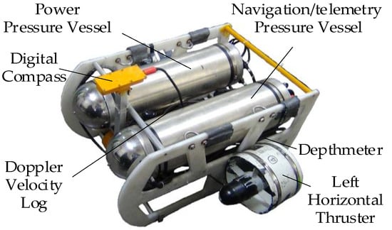
Figure 1.
Beaver II.
Beaver II takes the PC104 module as the core system and is equipped with a variety of expansion modules to realize data acquisition and analog/digital input and output. PC104 module runs VxWorks real-time operating system to ensure the real-time performance of AUV path planning, motion control, data transmission, and other functions. The control frequency is 5 Hz. Beaver II is divided into two parts: sensor system and actuator system. The specific configuration is as follows:
- Sensor System Configuration
To obtain AUV status information such as speed, angle and depth required for fault diagnosis, the sensors system configuration includes Doppler Velocity Log (Navquest 600 Micro); digital electronic compass (HMR3000); depth gauge (Cyt-151).
- b.
- Actuator System Configuration
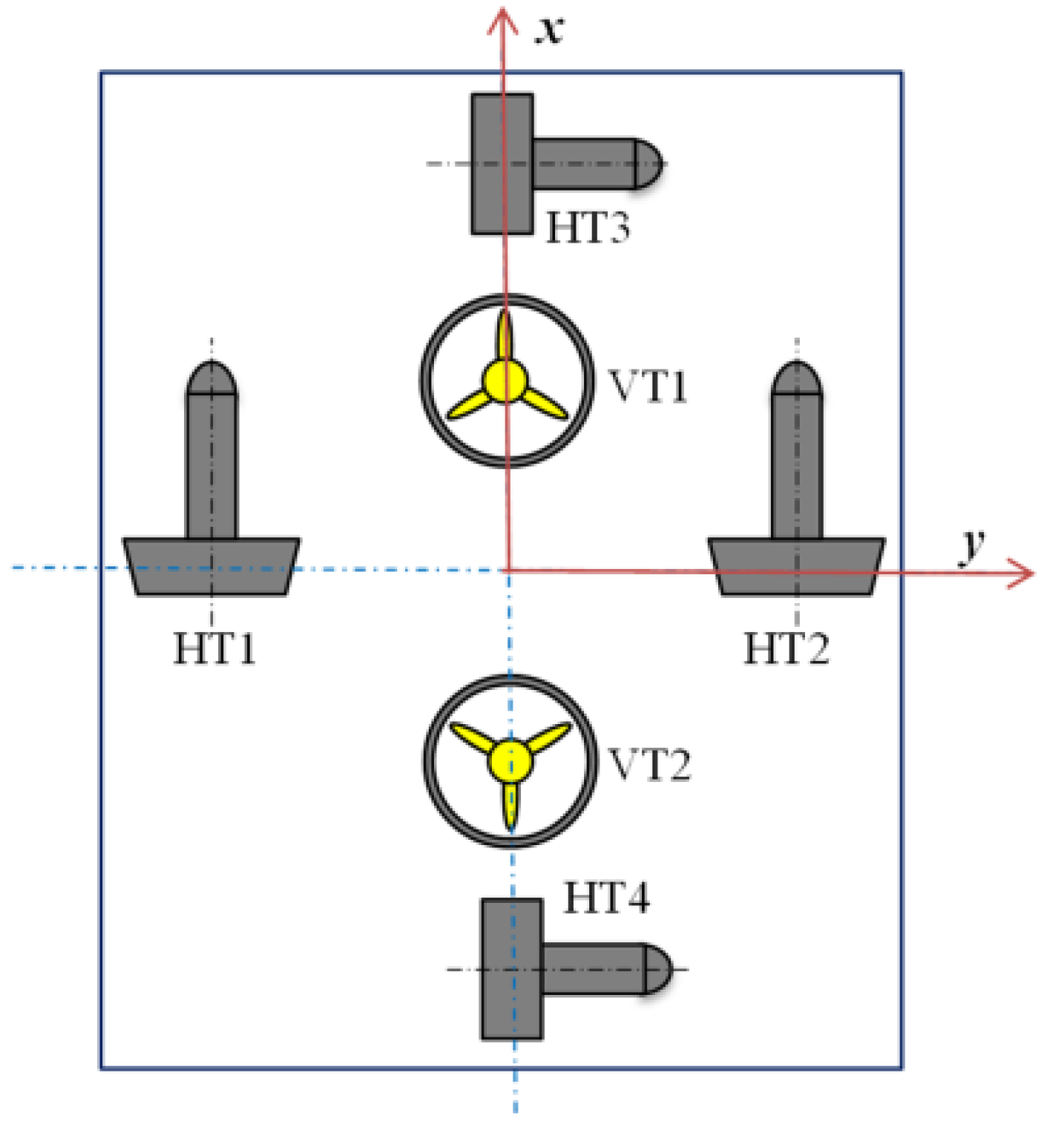
Beaver II is propelled by propellers, and the turning motion of the bow is realized by the lateral propeller and the differential between the two main propellers. The specific arrangement of the propeller is shown in Figure 2.

Figure 2.
Beaver II thruster layout.
In Figure 2, the propulsion system of Beaver II includes 6 propeller thrusters. The surge velocity is controlled by thrusters HT3 and HT4. The heading is controlled by thrusters HT1 and HT2. The depth is controlled by thrusters VT1 and VT2.
2.2. Experimental Environment
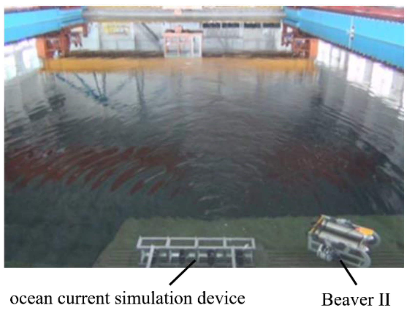
To simulate the influence of external interference such as ocean current on fault diagnosis as much as possible in the pool experimental environment, an ocean current simulation device used to produce ocean current was designed by the authors’ lab. The experimental pool and the device are shown in Figure 3.

Figure 3.
Experimental condition.
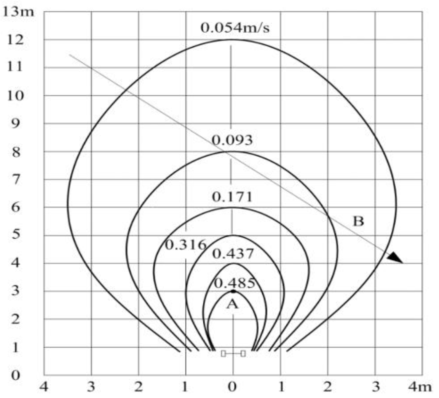
In Figure 3, the length, width, and depth of the experimental pool are 50 m, 30 m, and 10 m, respectively. The ocean current simulation device is composed of four thrusters (24 V, 200 W) arranged horizontally to simulate the current interference. During the experiment, the sampling period was 4 s, and the measured flow velocity is shown in Figure 4.
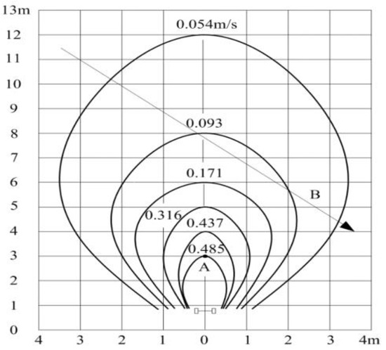
Figure 4.
Magnitude of ocean current.
In Figure 4, the ocean current simulation device is located 3 m below point A, and the AUV is driven along vector B.
2.3. Fault Simulation Method
The fault of AUV thrusters is generally manifested as output loss; that is, the actual output is less than the theoretical output. The greater the fault severity, the greater the difference between the theoretical output and the actual output. The reasons for the fault of AUV thrusters may include the entanglement of the propeller, the deformation and damage of the blade, the reduction of the performance of the motor driving the propeller, etc. In the experimental research of thruster faults, most of the thruster faults are made via software [24]. The specific method is as follows:
where is the actual input control voltage of the thruster, is the output voltage of the controller, and is the fault severity of thruster, and its variation range is (0%, 100%). 0% means no-fault, and 100% means the most serious fault with no thruster output. According to the relationship between and , the actual input control voltage of the thruster corresponding to each fault severity can be calculated. Adjusting can simulate different degrees of thruster fault severity.
3. Multi-Domain Fault Feature Extraction
Fault features are generally extracted in the time domain, frequency domain, and time-frequency domain, and several features can be extracted in each domain. In the past, fault features were generally extracted in a single domain of the above three domains. This idea is feasible for serious thruster fault, and there are many research results [16,17,18,19,20].
In this study, it was found that weak fault features extracted only in one certain domain have a poor effect, which directly affects the accuracy of subsequent fault severity identification. The reason for this is that the weak fault signal is weak, the strength of the fault feature is similar to the interference feature. Therefore, it is difficult to effectively extract weak fault features in a single domain to reflect the real essence of the fault. To accurately diagnose weak faults, fault features in multiple domains should be used effectively.
There are multiple input signals in this study, including surge velocity, yaw angle, control input, and tracking error, and there are multiple features in a domain (such as frequency domain) for one input signal. Therefore, there are many (up to dozens) features. Among the dozens of features, some of them may not meet the rule of monotonically increasing (or decreasing) with the increase of fault severity, and some of them meet this rule, but variation is very small. These features must be removed to provide as few and accurate features as possible for subsequent fault severity identification. For weak faults of AUV thrusters, no one has studied which features are useful.
Based on the above analysis, this paper proposes a multi-domain fault feature extraction method for weak fault feature extraction of AUV thrusters. The basic idea is as follows:
(1) Expand the domain of feature extraction. In the time domain, frequency domain, and time-frequency domain, the fault feature extraction method is studied.
(2) Improve the traditional feature calculation method. In the time domain, frequency domain, and time-frequency domain, the result obtained by the traditional calculation method may not meet the rule of monotonically increasing (or decreasing) with the increase of fault severity. In this paper, the traditional feature calculation method is improved.
(3) Optimize and select useful features. There are dozens of features in the time domain, frequency domain, and time-frequency domain, and many of them do not satisfy the monotonicity rule. If these are sent into fault severity identification without distinction, the accuracy of fault severity identification will be seriously affected. Therefore, to provide multi-source and accurate information for subsequent fault severity identification, based on the experimental results, the features that do not meet the monotonicity rule or have small variation are eliminated in the dozens of features in the time domain, frequency domain, and time-frequency domain, and the refined and accurate features are retained.
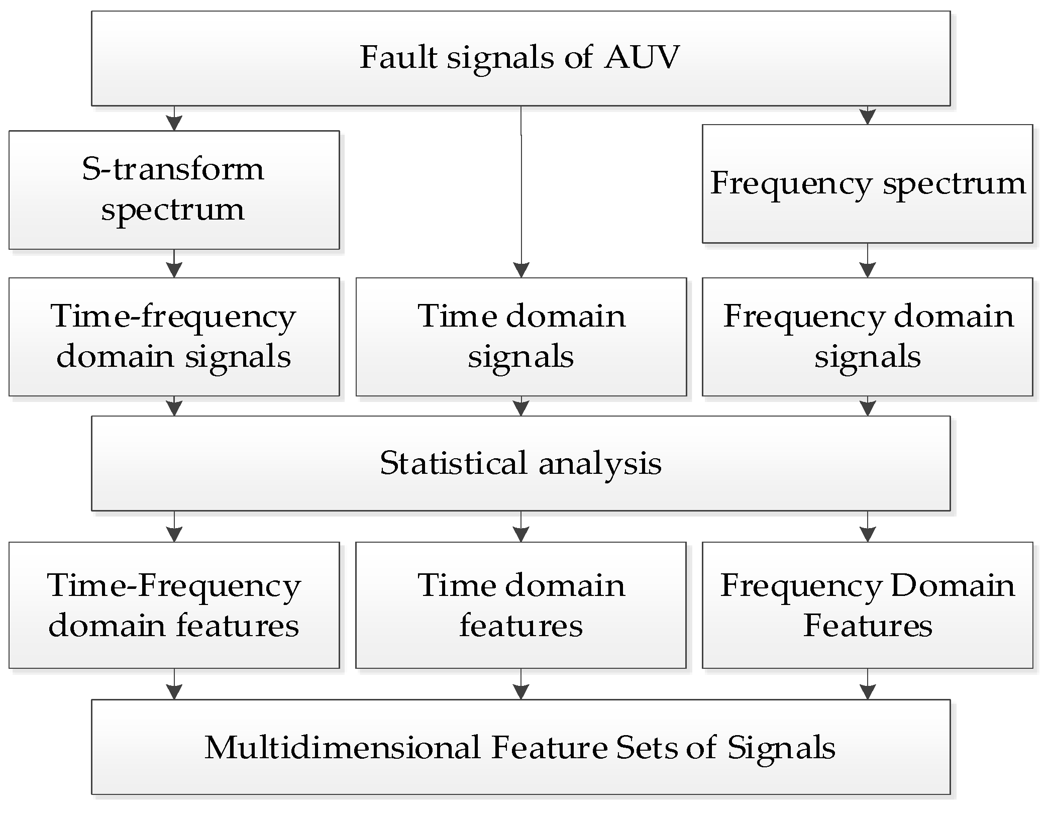
To summarize, the specific process of extracting multi-dimensional fault features in time domain, frequency domain, and time-frequency domain can be summarized, as shown in Figure 5.

Figure 5.
Process of multi-dimensional fault feature extraction.
4. Fault Features in Each Domain
This section describes the definition and calculation methods of fault features in each domain, so as to facilitate the analysis and refinement of each feature in subsequent sections.
4.1. Fault Features in the Time Domain
The discrete expression of the time domain signal is , and n is the number of sampling points. According to the literature [25,26], the six selected typical features in the time domain are as follows:
(1) Standard deviation (STD)
where .
(2) Root mean square (RMS)
(3) Fluctuation deviation (FLD)
(4) Kurtosis (KR)
where .
(5) Crest factor (CF)
with
where k is the number of short signals, and m is the length of the short signal, k = n/m; is the value of the i-th point within the j-th short signal, j = 1, 2, 3, …, k, i = 1, 2, 3, …, m.
(6) Shape factor (SF)
4.2. Fault Features in the Frequency Domain
According to the literature [27], the four typical features in the frequency domain after fast Fourier transform (FFT) are selected as follows:
(1) Mean frequency (MF)
(2) Frequency centroid (FC)
(3) Root mean square frequency (RMSF)
(4) Standard deviation frequency (STDF)
For Equations (9)–(12), is the frequency value and is the corresponding spectrum value, k = 1, 2, …, K, K is the total number of spectrum lines.
4.3. Fault Features in the Time-Frequency Domain
The three features in the time-frequency domain after S-transformation are as follows:
(1) Energy of probability (EOP)
where the energy operator is defined as the energy of the point in the S-transform spectrum. represents the average value of the energy operator of all points of the S-transform spectrum. is the number of energy operators, K is the number of spectral lines after FFT (fast Fourier transform), and n is the data length of the signal.
(2) Energy of local maximum (EOLM)
where represents the local energy entropy of all sub-regions of the S-transform spectrum, , a and b represent the length and width of sub-regions respectively, is the number of spectral lines after FFT, and n is the data length of the signal. The local energy entropy of each sub-region can be obtained by the sum of the energy operators of all points in the sub-region:
where , . The values of k and h are to ensure that the local energy entropy of all sub-regions can be obtained.
(3) Energy ratio (ER)
where , is given by Equation (15).
For Equations (13)–(16), the energy operator is as follows:
where is the frequency of the point in the S-transform spectrum, . is the amplitude of the point in the S-transform spectrum, .
In summary, there are 13 features in total, including 6 features in the time domain, 4 features in the frequency domain, and 3 features in the time-frequency domain.
As explained above, the weak fault diagnosis of the thruster studied in this paper has 4 input signals: surge velocity, yaw angle, control quantity, and tracking error; and each input signal can get 13 features, so there are 52 features in total. For the subsequent fault severity identification, it is not that the more features, the better. Instead, it is hoped to eliminate the features that do not satisfy the monotonicity law and the features with small changes and try to ensure that there are features in the three domains.
5. Analysis of Feature of Surge Velocity Signal
For the weak fault diagnosis of the thruster, there are 4 input signals: surge velocity, yaw angle, control quantity, and tracking error. To make the paper clear, this section takes the surge velocity signal as an example to study the change rule of its features in the time domain, frequency domain, and time-frequency domain. Aiming at the problem that the traditional feature calculation method in the frequency domain cannot obtain useful features, this paper proposes an improved feature calculation method verified by experiments.
5.1. Analysis of Fault Features in the Time Domain
The Beaver II is used to simulate different fault severity of thrusters (loss of effectiveness is 0%, 2%, 5%, 8%, and 10%), and the corresponding surge velocity signals are obtained. The length of the signal is 300. According to the feature calculation formula in Section 4, the 6 features, including FLD, KR, STD, RMS, CF, and SF in the time domain are obtained. The results are shown in Table 1.

Table 1.
Features of the surge velocity signal in the time domain for different fault severity.
From Table 1, as the fault severity increases (loss of effectiveness from 0% to 10%), FLD and KR show a monotonous increase, which is a usable feature; STD, RMS, CF, and SF do not show a monotonous increase (or decrease), which are unusable features.
Through the analysis of experimental data, the original 6 features in the time domain are reduced to two, which provides scientific and reasonable information for subsequent fault severity identification.
5.2. Analysis of Fault Features in the Frequency Domain
5.2.1. Results of Traditional Feature Calculation Method
The source of experimental data is the same as above. First, the frequency spectrum is obtained by FFT. The number of spectral lines is 300. Next, according to the feature calculation equations, the features, including MF, FC, RMSF, and STDF, in the frequency domain are obtained. The results are shown in Table 2.
Table 2 is analyzed as follows:
Table 2.
Features of the surge velocity signal in the frequency domain for different fault severity.
Table 2.
Features of the surge velocity signal in the frequency domain for different fault severity.
| Features | 0% | 2% | 5% | 8% | 10% |
|---|---|---|---|---|---|
| MF | 0.1979 | 0.1815 | 0.1418 | 0.1554 | 0.1324 |
| FC | 1.6623 | 1.6589 | 1.6616 | 1.6620 | 1.6686 |
| RMSF | 1.9165 | 1.9137 | 1.9199 | 1.9197 | 1.9218 |
| STDF | 0.9536 | 0.954 | 0.9619 | 0.9607 | 0.9535 |
As the fault severity increases (loss of effectiveness from 0% to 10%), none of the MF, FC, RMSF, and STDF show a monotonous increase (or decrease). Therefore, they are all unusable features.
5.2.2. The Improved Feature Calculation Methods
By analyzing the FFT of the weak fault signal of thrusters, it is found that the features of the amplitude variation signal of the weak fault signal in the frequency domain are more obvious than its features. Therefore, to enhance the features in the frequency domain of the signal, the three feature calculation methods of FC, RMSF, and STDF in the frequency domain are improved. Since the formula of MF does not contain a variable , MF will not be improved.
The implementation process of the improved methods are as follows:
The amplitude variation with more obvious feature variation replaces the amplitude in the original calculation formula, that is, amplitude variation replaces the amplitude in Equations (10)–(12).
The three improved features are respectively denoted as FCx, RMSFx, STDFx, and their formulae are as follows:
where , K is the number of frequencies of the signal after FFT, is the value of frequency.
The improved method and the traditional method were used to calculate the features of surge velocity signals in the frequency domain under different thruster faults. The comparison results are shown in Table 3.
Table 3 is analyzed as follows:
Table 3.
Comparison of feature extraction effect between improved method and traditional method.
Table 3.
Comparison of feature extraction effect between improved method and traditional method.
| Features | 0% | 2% | 5% | 8% | 10% | 20% | 30% |
|---|---|---|---|---|---|---|---|
| FC | 1.6623 | 1.6589 | 1.6616 | 1.6620 | 1.6686 | 1.6513 | 1.6587 |
| FCx | 0.1384 | 0.1261 | 0.1229 | 0.1251 | 0.1204 | 0.1123 | 0.0881 |
| RMSF | 1.9165 | 1.9137 | 1.9199 | 1.9197 | 1.9218 | 1.9110 | 1.9172 |
| RMSFx | 0.2463 | 0.2336 | 0.2238 | 0.2204 | 0.2176 | 0.1812 | 0.1379 |
| STDF | 0.9536 | 0.954 | 0.9619 | 0.9607 | 0.9535 | 0.9619 | 0.9615 |
| STDFx | 1.5677 | 1.5559 | 1.5436 | 1.5365 | 1.5261 | 1.4955 | 1.4542 |
For weak faults, FCx does not show a monotonous increase as the fault severity increases, so it is useless; RMSFx and STDFx meet the law of monotonicity as the fault severity increases, so they are useful. The original three features (FC, RMSF and STDF) are useless. In summary, 2 useful feature calculation methods illustrate the effectiveness of the improvements in this paper. Therefore, there are two useful features in the frequency domain for weak thruster faults: RMSFx and STDFx.
For serious faults (loss of effectiveness is 20% and 30%), RMSFx and STDFx also meet the law of monotonicity as the fault severity increases. It shows that the improved method is also applicable to serious faults. It further verifies the effect of the improved method in this paper.
5.3. Analysis of Fault Features in the Time-Frequency Domain
The experimental data is the same as Section 5.1. According to the feature calculation equation, the features, including EOP, EOLM and ER, in the time-frequency domain are obtained, and the results are shown in Table 4.
Table 4.
Features of surge velocity signal in the time-frequency domain for different fault severity.
With the increase of fault severity, EOP gradually decreases, EOLM and ER gradually increase. They all conform to the rule of monotonic change, which are useful features. Therefore, there are 3 useful features in the time-frequency domain for weak thruster faults, which are EOP, EOLM, and ER.
5.4. Analysis of Useful Features in Each Domain
Summarizing the useful features in the time domain, frequency domain, and time-frequency domain, the useful features of the surge velocity signal for weak fault diagnosis of the thruster are shown in Table 5, where √ means useful feature.
Table 5.
Useful features of surge velocity signal.
Table 5 shows that there are 16 features in the original time domain, frequency domain, and time-frequency domain. After the above analysis, 9 features that do not meet the rule are eliminated, and only 7 features are useful for the surge velocity signal, which provides refined and accurate information for subsequent fault severity identification.
5.5. Comprehensive Analysis of Features in Each Domain
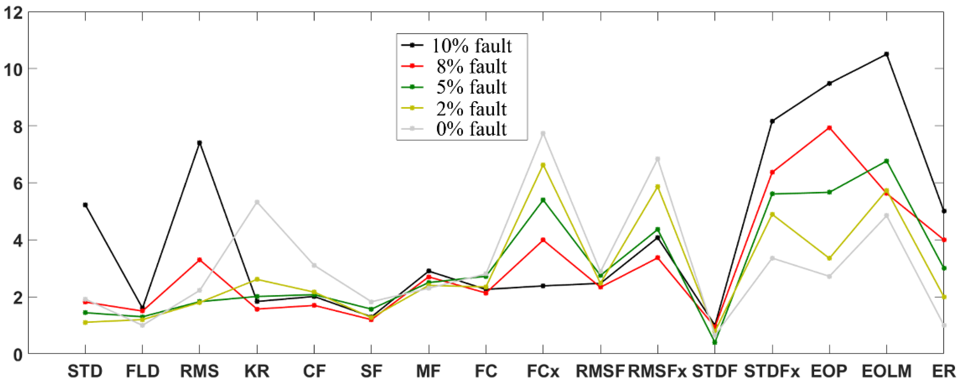
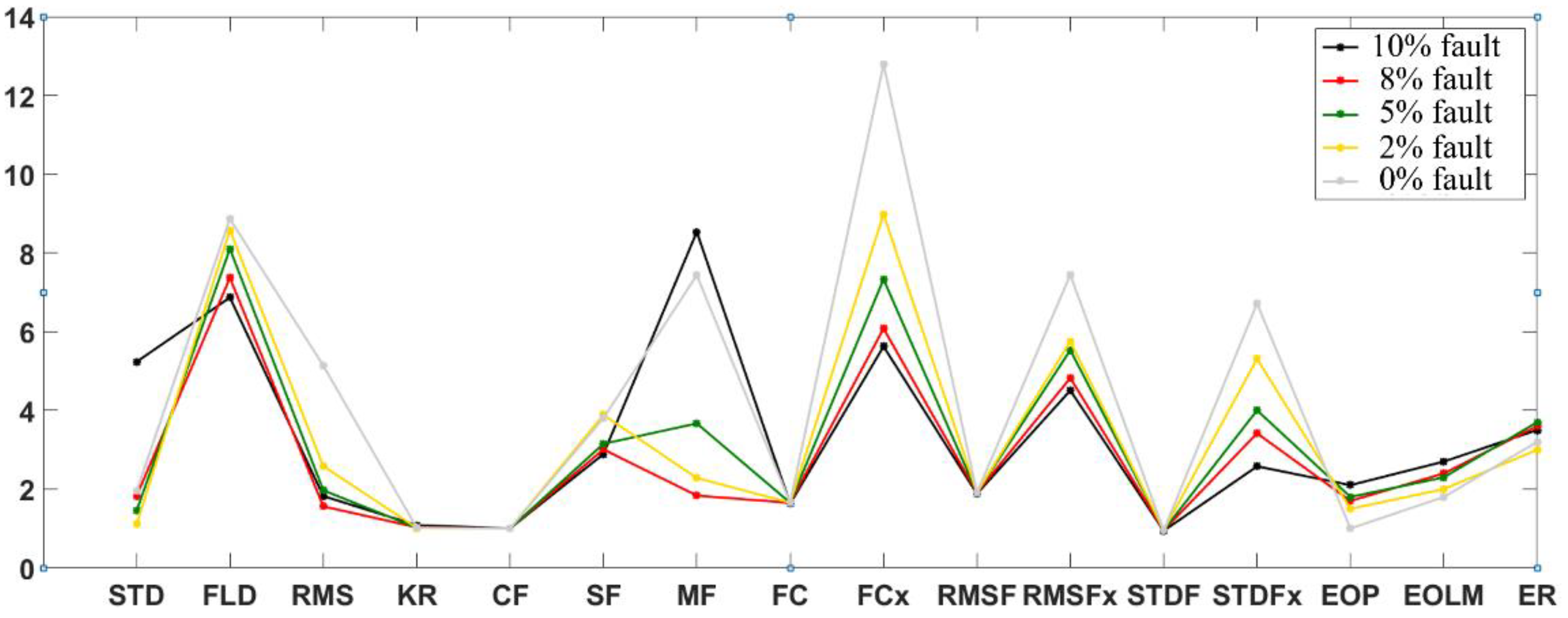
The useful features in the time domain, frequency domain, and time-frequency domain are summarized in the previous subsection, but the values of the features in each domain are different. To provide information on relative size between each feature for subsequent fault severity identification, all the feature values within the 3 domains are summarized in Figure 6. For a holistic analysis, the useless features are also included in Figure 6.
Figure 6 is analyzed as follows:
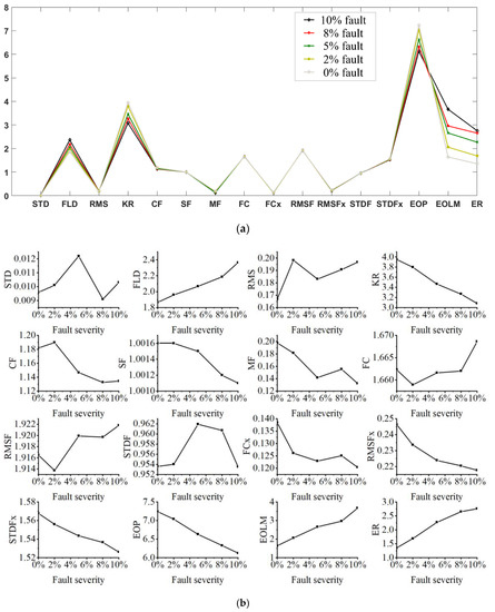
Figure 6.
Results of fault feature extraction of the surge velocity signal for weak fault severity: (a) Feature comparison; (b) All feature values.
Figure 6.
Results of fault feature extraction of the surge velocity signal for weak fault severity: (a) Feature comparison; (b) All feature values.
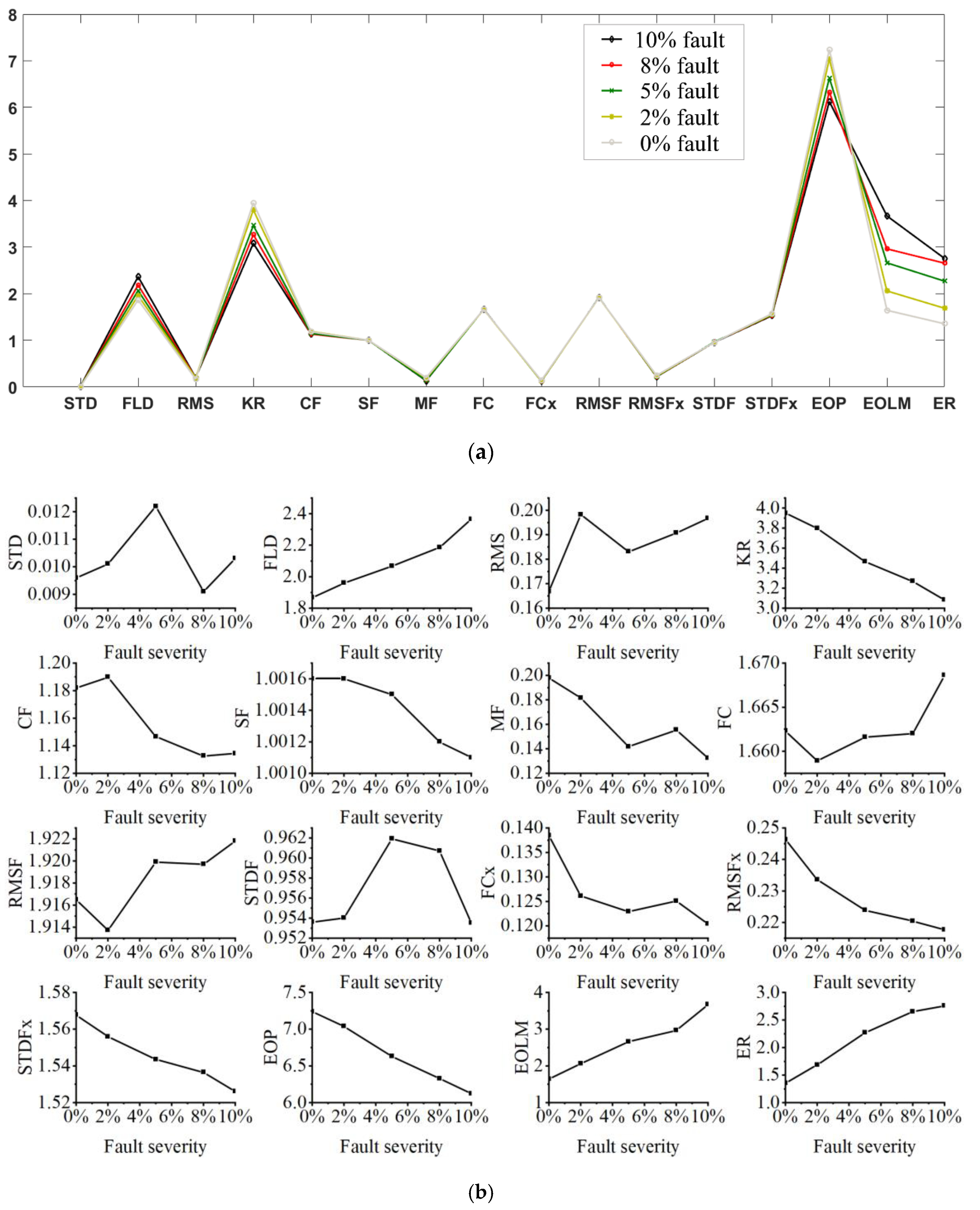
(1) Absolute Value
On the whole (absolute value), the features in the time-frequency domain are the largest and the features in the frequency domain are the smallest.
The size of each feature in each domain is further analyzed. The three useful features in the time-frequency domain (EOP, EOLM, ER) are the largest; the two useful features in the time domain (FLD, KR) are the second; the three useful features in the frequency domain (FCx, RMSFx, STDFx) are the smallest.
(2) The Difference of Feature Value with The Different Fault Severity
As the fault severity increases, the difference between the three useful features in the time-frequency domain is the largest; the difference between the two useful features in the time domain is the second; the difference between the three useful features in the frequency domain is the smallest.
Further analysis, as the fault severity increases, among the three features in the time-frequency domain, EOLM has the largest difference, ER is the second, and EOP is the smallest; among the two features in the time domain, the difference in KR is the largest, followed by the different in FLD. Compared with the features in the time-frequency domain and the time domain, the features in the frequency domain have the smallest difference with the increase of the fault severity.
Summary: The above-mentioned qualitative and quantitative analysis results of the absolute value of the features in different domains and the difference of feature value with the different fault severity have laid a good foundation for the feature fusion in the subsequent fault severity identification.
6. Determination of Useful Fault Features
In Section 5, the characteristics of the features of the surge velocity signals in each domain are studied, and then the useful features are determined. The input signal also includes the control quantity, yaw angle, and tracking error. The features of different input signals in each domain have their own unique characteristics. In this section, the characteristics of all features are studied, the useful features are determined, and the qualitative and quantitative analysis results are given.
Based on the developed method, the obtained features of the control quantity, tracking error, and yaw angle are shown in Figure 7, Figure 8 and Figure 9. The specific calculation process is the same as in Section 5, so the content of it is omitted here.
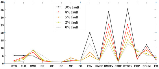
Figure 7.
Feature comparison of the control quantity signal for weak fault severity.

Figure 8.
Feature comparison of the tracking error signal for weak fault severity.
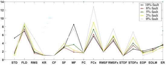
Figure 9.
Feature comparison of the yaw angle signal for weak fault severity.
To facilitate the analysis, the data in Figure 6, Figure 7, Figure 8 and Figure 9 are sorted into Table 6, Table 7, Table 8 and Table 9, respectively. The variation range in Table 6, Table 7, Table 8 and Table 9 refers to the variation of the feature when the fault severity is between 0% and 10%.
Table 6.
Useful features of the surge velocity signal.
Table 7.
Useful features of the control quantity.
Table 8.
Useful features of the tracking error.
Table 9.
Useful features of the yaw angle.
(1) Different input signals have different useful features in each domain.
Comparing Figure 6 and Figure 7, it was found that the useful features for the surge velocity signal are useless for the control quantity signal, such as KR. Therefore, the useful feature for the surge velocity signal cannot be directly used for the control quantity signal. It is necessary to find the useful features for each input signal.
(2) Different input signals have different average values of useful features in each domain.
Different input signals have a large difference in the average value of the useful features. The maximum is 21.769, the minimum is 1.351, and the difference between the two is 20.418. Therefore, in the subsequent data fusion, this problem should be dealt with.
(3) As the fault severity changes, different input signals have different variation ranges of useful features in each domain.
For the fault with 0% to 10% loss of effectiveness, the variation range of the useful features of different input signals is different. The maximum is 22.995, the minimum is 0.450, and the difference between the two is 22.545. Therefore, in the subsequent data fusion, this problem should be dealt with.
(4) Aiming at the problem that the traditional feature calculation method cannot obtain the useful feature in the frequency domain, an improved method is proposed in this paper. The effectiveness of the improved method in this paper has been verified in each domain. On the other hand, without the improved method in this paper, only the useful features in the time domain and time-frequency domain can be obtained. The improved method in this paper can obtain the useful features in the frequency domain, increasing the useful features in one domain (frequency domain).
(5) Through Table 6, Table 7, Table 8 and Table 9, we can determine the size of each feature itself, as well as the relative size of each useful feature, which provides effective quantitative information for fault fusion in subsequent fault severity identification.
Discussion of experimental results:
(1) This paper takes the open-frame AUV as the experimental object. The moving speed of an open-frame AUV is relatively low. For streamlined AUV with relatively high speed, the fault features determined in this paper may not be applicable. Therefore, it needs to be further adjusted in combination with the data of the streamlined AUV, but the idea is the same as this paper.
(2) Limited by the depth of the pool, this paper analyzes the variation law of fault features by the data obtained from the constant speed directional experiment of AUV in the horizontal direction. Whether this law is applicable to the experimental data of heave movement needs to be further studied.
(3) AUV data obtained from the experimental pool in this paper have some differences compared with the real sea trial data. The useful features and their order of magnitude should be further refined in combination with sea trial data.
7. Conclusions
Aiming at the problem of weak fault feature extraction of AUV thrusters, this paper systematically studies the characteristics and changing laws of fault features in the time domain, frequency domain, and time-frequency domain. The 32 features that do not meet the monotonicity rule are eliminated from the original 52 features, and only 20 scientifically reasonable features are retained. Among the 20 retained features, the order of magnitude of each feature amount is given. It effectively reduces the number of useless features and provides refined and accurate information for subsequent fault severity identification. At the same time, for the problem that the traditional calculation method of feature cannot effectively extract the fault features in the frequency domain so that there is no useful feature in the frequency domain, this paper proposes an improved method. The experimental results show that the frequency domain features with monotonic variation characteristics can be obtained based on the improved method, which increases the number of fault features in the frequency domain. It provides effective qualitative and quantitative information for subsequent fault severity identification
However, there are some limitations in this paper: This paper takes the open-frame AUV as the experimental object. The moving speed of an open-frame AUV is relatively low. For a streamlined AUV with relatively high speed, the fault features determined in this paper may not be applicable. Therefore, it needs to be further adjusted in combination with the data of the streamlined AUV. Limited by the depth of the pool, this paper analyzes the variation law of fault features by the data obtained from the constant speed directional experiment of an AUV in the horizontal direction. Whether this law is applicable to the experimental data of heave movement needs to be further studied. AUV data obtained from the experimental pool in this paper have some differences compared with the real sea trial data. The useful features and their order of magnitude should be further refined in combination with sea trial data.
Author Contributions
Conceptualization, D.Y. and C.Z.; methodology, D.Y.; software, C.Z.; validation, D.Y., C.Z. and X.L.; formal analysis, D.Y. and C.Z.; investigation, D.Y. and C.Z.; resources, X.L. and M.Z.; data curation, C.Z. and X.L.; writing—original draft preparation, D.Y.; writing—review and editing, X.L. and M.Z.; visualization, X.L.; supervision, X.L.; project administration, M.Z.; funding acquisition, M.Z. All authors have read and agreed to the published version of the manuscript.
Funding
This research was funded by National Natural Science Foundation of China under Grant 51839004.
Institutional Review Board Statement
Not applicable.
Informed Consent Statement
Not applicable.
Data Availability Statement
Not applicable.
Conflicts of Interest
The authors declare no conflict of interest.
References
- Yu, C.; Xiang, X.; Maurelli, F.; Zhang, Q.; Zhao, R.; Xu, G. Onboard system of hybrid underwater robotic vehicles: Integrated software architecture and control algorithm. Ocean Eng. 2019, 187, 106121. [Google Scholar] [CrossRef]
- Dearden, R.; Ernits, J. Automated fault diagnosis for an autonomous underwater vehicle. IEEE J. Ocean Eng. 2013, 38, 484–499. [Google Scholar] [CrossRef]
- Zhu, C.; Huang, B.; Zhou, B.; Su, Y.M.; Zhang, E.H. Adaptive model-parameter-free fault-tolerant trajectory tracking control for autonomous underwater vehicles. ISA Trans. 2021, 114, 57–71. [Google Scholar] [CrossRef] [PubMed]
- Brito, M.; Griffiths, G.; Ferguson, J.; Hopkin, D.; Mills, R.; Pederson, R.; Macneil, E. A behavioral probabilistic risk assessment framework for managing autonomous underwater vehicle deployments. J. Atmos. Ocean Technol. 2012, 29, 1689–1703. [Google Scholar] [CrossRef] [Green Version]
- Wang, H.; Chen, J. Performance degradation assessment of rolling bearing based on bispectrum and support vector data description. J. Vib. Control 2014, 20, 2032–2041. [Google Scholar] [CrossRef]
- Zhang, M.J.; Wang, Y.J.; Xu, J.A.; Liu, Z.C. Thruster fault diagnosis in autonomous underwater vehicle based on grey qualitative simulation. Ocean Eng. 2015, 105, 247–255. [Google Scholar] [CrossRef]
- Liu, W.X.; Wang, Y.J.; Liu, X.; Zhang, M.J. Weak thruster fault detection for AUV based on stochastic resonance and wavelet reconstruction. J. Cent. South Univ. 2016, 23, 2883–2895. [Google Scholar] [CrossRef]
- Vu, M.T.; Thanh, H.L.N.N.; Huynh, T.T.; Thang, Q.; Duc, T.; Hoang, Q.D.; Le, T.H. Station-Keeping Control of a Hovering Over-Actuated Autonomous Underwater Vehicle Under Ocean Current Effects and Model Uncertainties in Horizontal Plane. IEEE Access 2021, 9, 6855–6867. [Google Scholar] [CrossRef]
- Vu, M.T.; Le, T.H.; Thanh, H.L.N.N.; Huynh, T.T.; Van, M.; Hoang, Q.D.; Do, T.D. Robust Position Control of an Over-actuated Underwater Vehicle under Model Uncertainties and Ocean Current Effects Using Dynamic Sliding Mode Surface and Optimal Allocation Control. Sensors 2021, 21, 747. [Google Scholar] [CrossRef] [PubMed]
- Dos Santos, C.H.F.; Cardozo, D.I.K.; Reginatto, R.; De Pieri, E.R. Bank of controllers and virtual thrusters for fault-tolerant control of autonomous underwater vehicles. Ocean Eng. 2016, 121, 210–223. [Google Scholar] [CrossRef]
- Liu, W.; Zhang, M.; Wang, Y. Weak thruster fault prediction method for autonomous underwater vehicles based on grey model. Proc. Inst. Mech. Eng. Part I J. Syst. Control Eng. 2019, 233, 348–356. [Google Scholar] [CrossRef]
- Yin, B.; Yao, F.; Wang, Y.; Zhang, M.; Zhu, C. Fault degree identification method for thruster of autonomous underwater vehicle using homomorphic membership function and low frequency trend prediction. Proc. Inst. Mech. Eng. Part C J. Mech. Eng. Sci. 2019, 233, 1426–1440. [Google Scholar] [CrossRef]
- Sun, Y.S.; Ran, X.R.; Li, Y.M.; Zhang, G.C.; Zhang, Y.H. Thruster fault diagnosis method based on Gaussian particle filter for autonomous underwater vehicles. Int. J. Nav. Archit. Ocean Eng. 2016, 8, 243–251. [Google Scholar] [CrossRef] [Green Version]
- Qin, H.; Chen, H.; Sun, Y.; Chen, L. Distributed finite-time fault-tolerant containment control for multiple ocean Bottom Flying node systems with error constraints. Ocean Eng. 2019, 189, 106341. [Google Scholar] [CrossRef]
- Chu, Z.; Meng, F.; Zhu, D.; Luo, C. Fault reconstruction using a terminal sliding mode observer for a class of second-order MIMO uncertain nonlinear systems. ISA Trans. 2020, 97, 67–75. [Google Scholar] [CrossRef] [PubMed]
- Gao, M.; Yu, G.; Li, C. Incipient Gear Fault Detection Using Adaptive Impulsive Wavelet Filter Based on Spectral Negentropy. Chin. J. Mech. Eng. 2022, 35, 10. [Google Scholar] [CrossRef]
- Xia, S.; Zhou, X.; Shi, H.; Li, S.; Xu, C. A fault diagnosis method based on attention mechanism with application in Qianlong-2 autonomous underwater vehicle. Ocean Eng. 2021, 233, 109049. [Google Scholar] [CrossRef]
- She, B.; Wang, X. A hidden feature label propagation method based on deep convolution variational autoencoder for fault diagnosis. Meas. Sci. Technol. 2022, 33, 055107. [Google Scholar] [CrossRef]
- Jiang, Y.; He, B.; Guo, J.; Lv, P.; Mu, X.; Zhang, X.; Yu, F. Actuator Weak Fault Diagnosis in Autonomous Underwater Vehicle Based on Tri-Stable Stochastic Resonance. Appl. Sci. 2020, 10, 2048. [Google Scholar] [CrossRef] [Green Version]
- Chen, G.; Yan, C.; Meng, J.; Wang, H.; Wu, L. Improved VMD-FRFT based on initial center frequency for early fault diagnosis of rolling element bearing. Meas. Sci. Technol. 2021, 32, 115024. [Google Scholar] [CrossRef]
- Liu, W.; Wang, Y.; Yin, B.; Liu, X.; Zhang, M. Thruster fault identification based on fractal feature and multiresolution wavelet decomposition for autonomous underwater vehicle. Proc. Inst. Mech. Eng. Part C J. Mech. Eng. Sci. 2016, 231, 2528–2539. [Google Scholar] [CrossRef]
- Zhang, M.J.; Yin, B.J.; Liu, W.X.; Liu, X. Thruster fault feature extraction for autonomous underwater vehicle in time-varying ocean currents based on single-channel blind source separation. Proc. Inst. Mech. Eng. Part I J. Syst. Control Eng. 2016, 230, 46–57. [Google Scholar] [CrossRef]
- Lv, T.; Chen, Z.; Yao, F.; Zhang, M. Fault feature extraction method based on optimized sparse decomposition algorithm for AUV with weak thruster fault. Ocean Eng. 2021, 233, 109013. [Google Scholar] [CrossRef]
- Zhang, M.; Wu, J.; Wang, Y. A method of multi-sensor simultaneous faults detection for autonomous underwater vehicle. Robot 2010, 32, 298–305. [Google Scholar] [CrossRef]
- Lei, Y.G.; He, Z.J.; Zi, Y.Y. Application of an intelligent classification method to mechanical fault diagnosis. Expert Syst. Appl. 2009, 36, 9941–9948. [Google Scholar] [CrossRef]
- Samanta, B.; Al-Balushi, K.R. Artificial neural network based fault diagnostics of rolling element bearings using time-domain features. Mech. Syst. Signal Process. 2003, 17, 317–328. [Google Scholar] [CrossRef]
- Wang, Y.; Jiang, Y.; Kang, S. The application of time domain and frequency domain statistical factors on rolling bearing performance degradation assessment. Comput. Model. New Technol. 2014, 18, 192–198. [Google Scholar]


Publisher’s Note: MDPI stays neutral with regard to jurisdictional claims in published maps and institutional affiliations. |
© 2022 by the authors. Licensee MDPI, Basel, Switzerland. This article is an open access article distributed under the terms and conditions of the Creative Commons Attribution (CC BY) license (https://creativecommons.org/licenses/by/4.0/).