Mechanism Analysis of Time-Dependent Characteristic of Dynamic Errors of Machine Tools

Abstract

The Dynamic Errors (DEs) of individual axes present Time-dependent Characteristics (TDCs) because the setpoints, as the input of the servo feed system, change in velocity, acceleration and jerk during the feed motion. Deep insight into the TDC contributes to the effective control of DEs. However, up to now, mechanism analysis about the TDCs of DEs are indistinct and inadequate due to a lack of analysis on the TDC of setpoint frequency. So, in this study, the mechanism of the TDC of DE is investigated by extracting the TDC of setpoint frequency. Firstly, the servo dynamics model is established for presenting the DE and its respective components, the Dynamic Error Inside Servo-loop (DEIS) (tracking error) and the Dynamic Error Outside Servo-loop (DEOS) under to and fro motions. Secondly, time–frequency analysis is carried out on the setpoints of the to and fro motions to present a TDC of setpoint frequency which is described as the Time-dependent Setpoint Bandwidth (TDSB) and the Time-dependent Potential Excitation (TDPE). Finally, the correlation between the TDSBs and DEISs and the correlation between the TDPEs and DEOSs are investigated, respectively. On these bases, the mechanism of the TDC of DE is analyzed. The results show that the TDSB, which is related to the acceleration of setpoints, accounts for the TDC of the DEIS; that the TDPE, which is related to the jerk of setpoints, accounts for the TDC of the DEOS in vibration-form; and that the TDC of transient-form DEOS is determined by the change in acceleration of the setpoints.

1. Introduction

The basic function of multi-axis CNC machine tools is to drive the tool and workpiece in order to accurately realize the desired tool trajectory. This basic function needs to be executed by both the CNC system and the servo feed systems. Firstly, the tool trajectory (represented by G code) is input into the CNC system for interpolation. After interpolation, the CNC system generates the setpoints trajectory (synthesized by the setpoints of each axis), then outputs the setpoints trajectory to the servo feed systems. Secondly, the servo feed systems receive the setpoints trajectory and perform the feed motions to synthesize the actual trajectory, which directly decides the machining accuracy of the multi-axis CNC machine tool.

To guarantee the accuracy of the actual trajectory, both the deviation from the setpoints trajectory to the tool trajectory and the deviation of the actual trajectory from the setpoints trajectory should be guaranteed by the interpolation of the CNC system and the control of servo feed systems. When it comes to the interpolation of the CNC system, deviation is limited by setting geometric constraints such as chord error. Meanwhile, in the control of servo feed systems, it is generally limited by controlling the Dynamic Error (DE) of each axis, as shown in Figure 1. Compared with the chord error, the control of the DE of individual axes is more difficult due to the complex causes of deviation.

The DE of individual axes is the deviation of the actual position of the effector end of the servo feed system from the setpoints position. Recently, Lyu et al. [1] divided the DE into the Dynamic Error Inside Servo-loop (DEIS) (tracking error) and the Dynamic Error Outside Servo-loop (DEOS). The DEIS is the deviation of the feedback detection position from the setpoints position. The DEOS is the deviation of the actual position of the effector end from the feedback detection position. Because the setpoints, as the input of the servo feed system, change in velocity, acceleration and jerk during the feed motion, the DEs of individual axes present a Time-dependent Characteristic (TDC). To control the accuracy of the actual trajectory, it is crucial that the DE should be reduced to a sufficient degree at every time point.

There have been numerous studies concerning on the control of DEs. The progress made over the last few decades has been reviewed by Altintas et al. [2], Huo and Poo [3], Tang and Landers [4], Uriarte el al. [5], Oomen [6], Meng et al. [7] and Lyu et al. [1]. The DE is related to both the servo dynamics and the setpoints. The servo dynamics can usually be evaluated by using a Bode Diagram. This employs frequency-domain indexes, such as servo bandwidth and resonance peaks, to describe the responsiveness and resonance suppression of the servo feed system against the input of setpoints. When the servo dynamics are optimized and determined, the DE is decided by the setpoints. The TDC of setpoint frequency determines the TDC of the DE.

Thus far, the time-domain and frequency-domain methods have been used to analyze and evaluate the setpoints. As for the time-domain method, the extreme velocity, acceleration and jerk can be directly observed through the setpoints sequence, and this can be used to judge whether it is outside of the scope of limitation [8,9,10,11,12,13,14]. However, the time-domain method cannot evaluate the TDC of setpoint frequency.

As for the frequency-domain method, Smith [15] analyzed the rectangular, trapezoid and triangular acceleration setpoints via FFT analysis. He found out that the setpoint bandwidth of these three setpoints decrease in turn. In addition, through FFT analysis, the excitation frequencies can also be compared. Altintas et al. [2] compared rectangular, trapezoid and cubic acceleration setpoints. They found out that the second order continuous jerk of the latter has the least potential excitation frequencies and, accordingly, has the least mechanical vibration. The setpoint bandwidth and high frequency components can be presented through the frequency-domain method. This can be used to evaluate whether the setpoints can be responded to by the servo feed system and whether the mechanical vibrations can be excited by the setpoints. However, the frequency-domain method can only analyze the whole setpoints and cannot evaluate the TDC of setpoint frequency.

Up to now, few analyses have focused on the TDC of setpoint frequency, which has resulted in the lack of mechanism analysis in relation to the TDC of DE.

Time–frequency analysis is a modern branch of harmonic analysis. It analyzes a signal in both the time- and frequency- domains simultaneously and is broadly studied and used in image processing, signal analysis and communication theory, and so on. However, in motion control, only a few related studies have been conducted to date. Rotoariu et al. [16] introduced time–frequency analysis into motion control. They integrated time–frequency analysis in terms of the Wigner distribution with the field of Iterative Learning Control (ILC) for controlling a wafer stage. The Wigner distribution is successfully used to analyze tracking errors and to design a time–frequency adaptive filter in ILC [17,18], which, as Rotoariu et al. showcase, increases the feasibility and prospects of using time–frequency analysis in motion control. Alkafafi [19] developed a method based on a wavelet analysis to identify the critical oscillation regions by using the vibrational contour error signal, which makes use of the redundant representation of the wavelet transform and its ability to localize signal information on the time-scale grid. In the studies mentioned above, the tracking error and the contour error signals are analyzed using the time–frequency method. Time–frequency analysis directly aimed at the setpoints has not yet been reported.

In this study, the time–frequency domain method was employed to extract the TDC of setpoint frequency and to analyze the TDC of DE. Firstly, the servo dynamics model for the ball screw servo feed system of the X-axis cascading with the Z-axis of the three-axis machine tool was established for the purpose of presenting both the DEIS and DEOS. By inputting the setpoints of to and fro motions into the model, the DEs, DEISs, DEOSs could be illustrated. Secondly, time–frequency analysis was carried out on the setpoints of to and fro motions to present the TDC of setpoint frequency. Using this analysis, the Time-dependent Setpoint Bandwidths (TDSBs) and the Time-dependent Potential Excitations (TDPEs) of the setpoints of to and fro motions were extracted. Finally, the correlation between the TDSBs and DEISs and the correlation between the TDPEs and DEOSs were investigated, respectively. On these bases, the mechanism of the TDC of DE was analyzed.

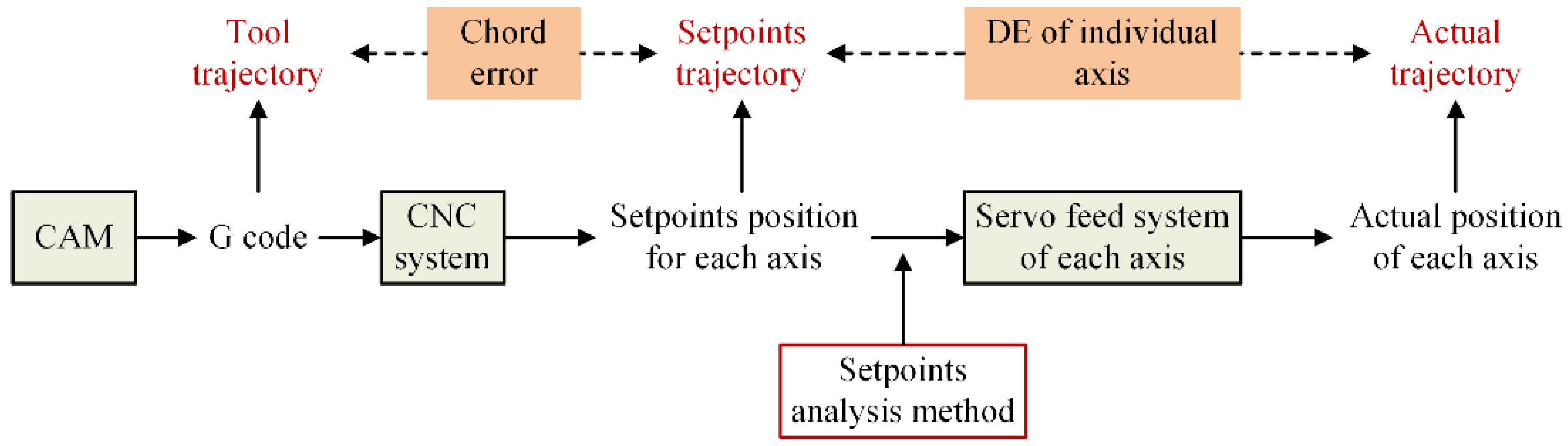
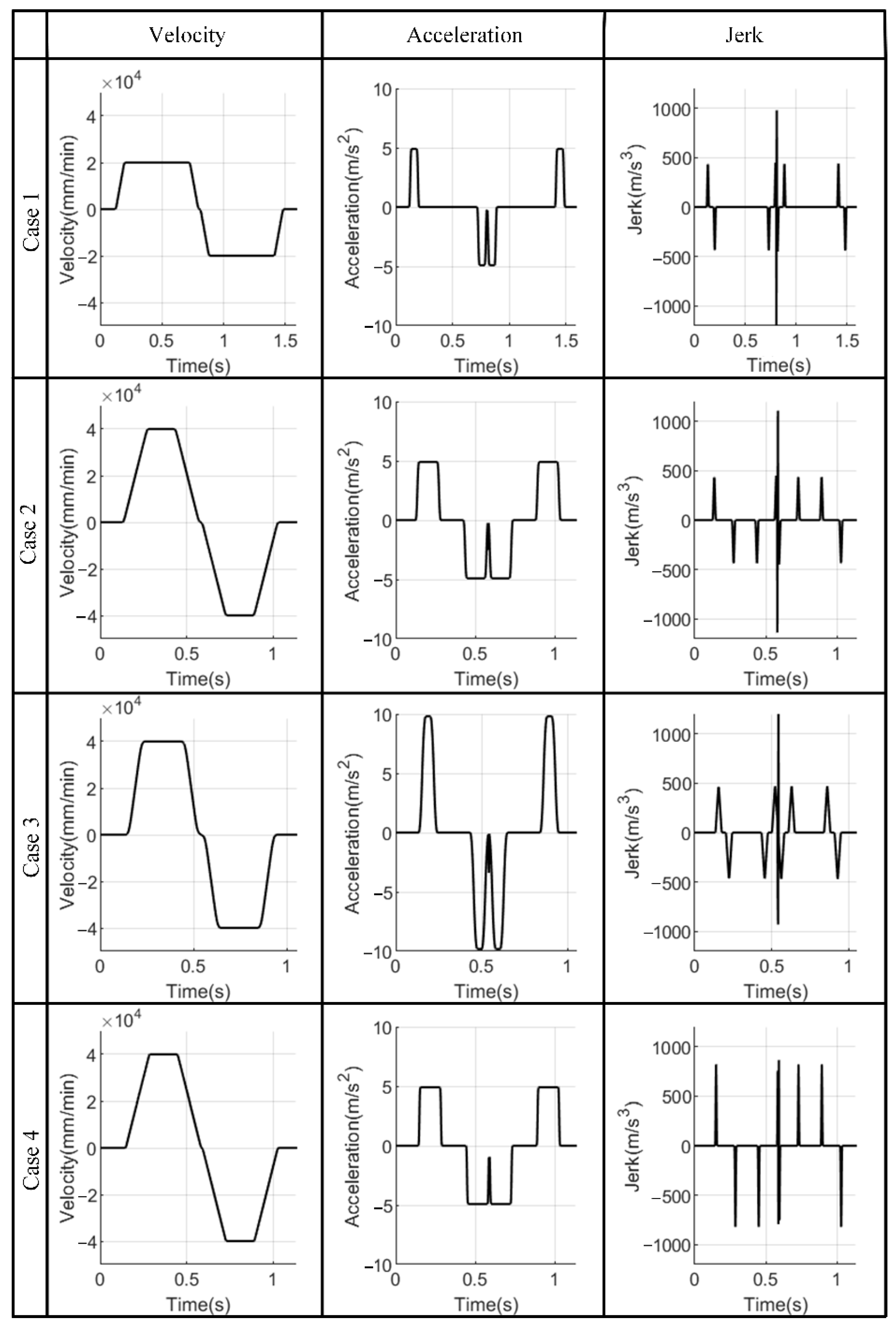
2. The DEs of an Individual Axis under To and Fro Motions

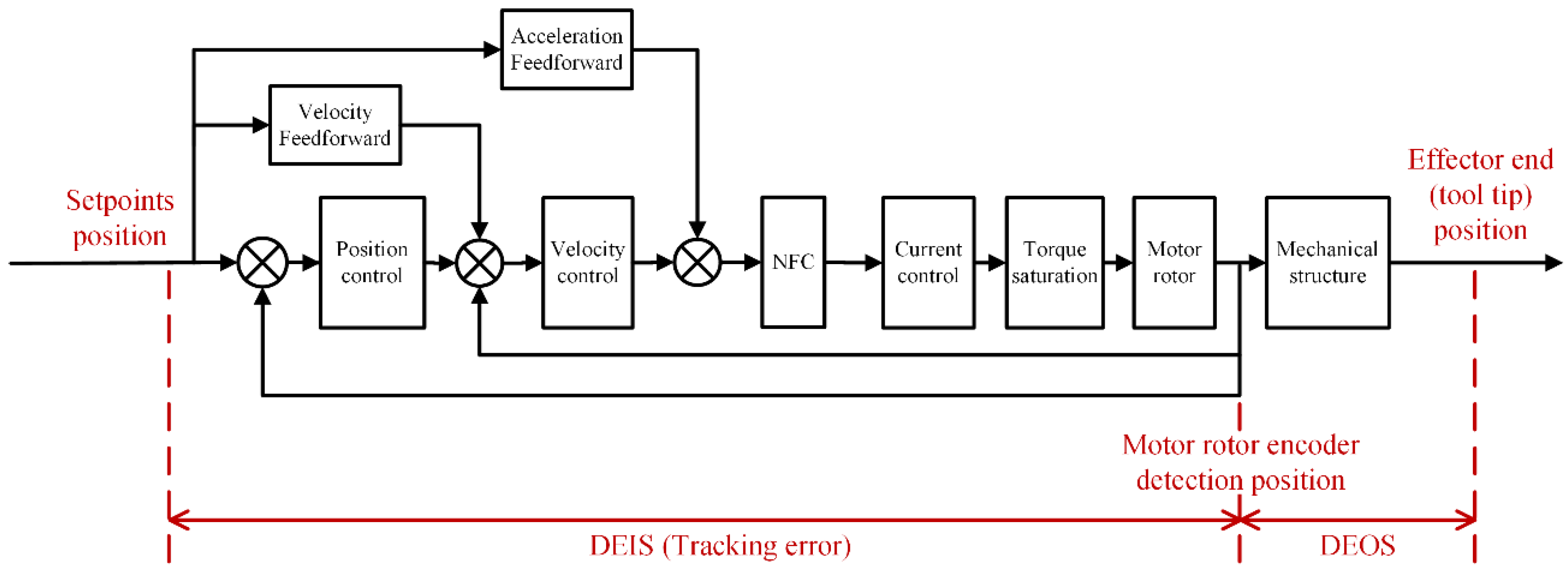
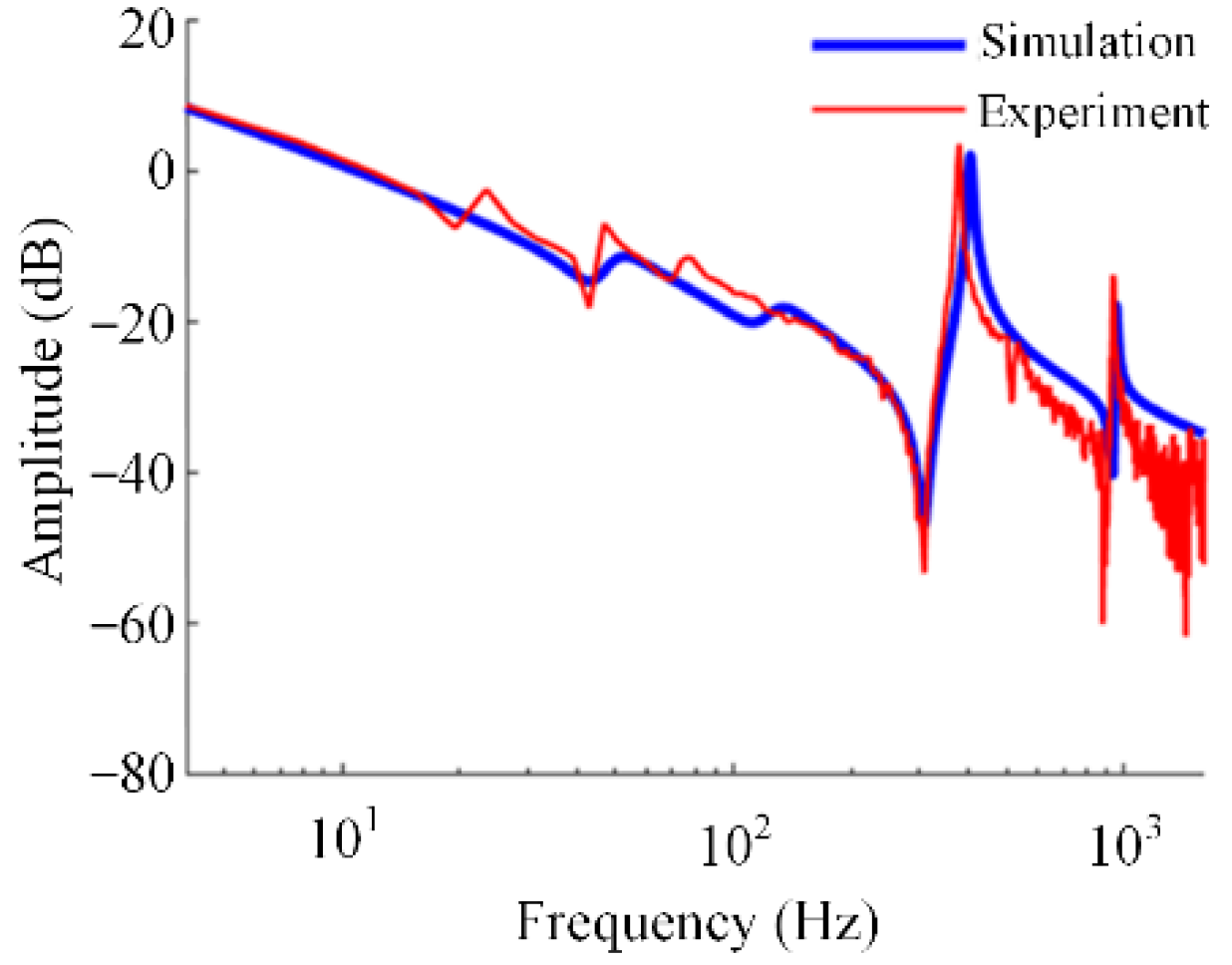
2.1. The Mechanical Dynamics and Servo Control Model of the Individual axis

An individual axis of the three-axis milling machine was employed for investigating DEs. For presenting both DEIS and DEOS, the X-axis which is cascaded with the Z-axis was selected to establish the mechanical dynamics model. The X-axis was a ball screw servo feed system. The equivalent dynamics model is shown in Figure 2.

In Figure 2, the screw is equivalent to the two-inertia-spring-damping system. The motor is equivalent to the rotor inertia. The coupling is equivalent to the torsion spring. The slide block, the lead screw nut and the lead screw bearing are equivalent to the spring damping unit. The carriage connecting with the X- and Z-axes is equivalent to the torsion spring damping unit.

The ball screw servo feed mechanical system can be formulated using Lagrange’s method. The kinetic energy of the system can be expressed as:

$$T=\frac{1}{2}{J}_1{\dot{\theta }}_1{}^2+\frac{1}{2}{J}_2{\dot{\theta }}_2{}^2+\frac{1}{2}{J}_3{\dot{\theta }}_3{}^2+\frac{1}{2}{m}_a{\dot{x}}_a{}^2+\frac{1}{2}{m}_t{\left({\dot{x}}_a-L_1{\dot{\theta }}_t\right)}^2+\frac{1}{2}{J}_t{\dot{\theta }}_t{}^2$$

(1)

where T is the kinetic energy of the system; J₁ is the inertia of the motor; J₂ is the first inertia of the ball screw; J₃ is the second of inertia of the ball screw; J_t is the inertia of the Z-axis; θ₁ is motor’s rotation angle; θ₂ is the rotation angle of the ball screw; θ₃ is nut’s rotation angle; θ_t is the rotation angle of the Z-axis; x_a is the displacement of the saddle; m_a is the mass of the saddle; and m_t is the mass of the Z-axis.

The potential energy of the system is:

$$V=\frac{1}{2}{K}_1{\left({\theta }_1-{\theta }_2\right)}^2+\frac{1}{2}{K}_2{\left({\theta }_2-{\theta }_3\right)}^2+\frac{1}{2}{K}_a{\left({\theta }_3{r}_g-x_a\right)}^2+\frac{1}{2}{K}_t{\theta }_t{}^2$$

(2)

where V is the potential energy of the system; K₁ is the equivalent torsion stiffness of the coupling; K₂ is the equivalent torsion stiffness of the ball screw; K_a is the axial equivalent linear stiffness of the system; K_t is the equivalent torsion stiffness between series structures; and r_g is transmission ratio of the ball screw.

The dissipation function can be written as:

$$F=\frac{1}{2}{C}_1{\left({\dot{\theta }}_1-{\dot{\theta }}_2\right)}^2+\frac{1}{2}{C}_2{\left({\dot{\theta }}_2-{\dot{\theta }}_3\right)}^2+\frac{1}{2}{C}_a{\left({\dot{\theta }}_3{r}_g-{\dot{x}}_a\right)}^2+\frac{1}{2}{C}_{rf}{\dot{\theta }}_1{}^2+\frac{1}{2}{C}_{lf}{\dot{x}}_a{}^2+\frac{1}{2}{C}_t{\dot{\theta }}_t{}^2$$

(3)

where F is dissipation energy of the system; C₁ is the damping coefficient of the coupling; C₂ is the damping coefficient of the ball screw; C_a is the axial damping coefficient of the system; C_rf is the viscous friction coefficient of the bearing; and C_lf is the viscous friction coefficient of the guide and block pair.

Let

$$O=T-V$$

(4)

then

$$\frac{\partial }{\partial t}\left(\frac{\partial O}{\partial {\dot{q}}_i}\right)-\frac{\partial O}{\partial q_i}=Q_i-\frac{\partial F}{\partial {\dot{q}}_i}$$

(5)

In Equation (5) the general coordinates q_i is defined as:

$$q_i={\left\{\begin{array}{ccccc}{\theta }_1& {\theta }_2& {\theta }_3& x_a& {\theta }_t\end{array}\right\}}^T$$

(6)

The general forces Q_i is defined as:

$$Q_i={\left\{\begin{array}{ccccc}{T}_m& 0& 0& 0& 0\end{array}\right\}}^T{}_i$$

(7)

The dynamic equations of the feed system can be obtained as:

$$\{\begin{array}{l}{J}_1{\ddot{\theta }}_1+C_1\left({\dot{\theta }}_1-{\dot{\theta }}_2\right)+C_{rf}{\dot{\theta }}_1+K_1\left({\theta }_1-{\theta }_2\right)=T_m\\ J_2{\ddot{\theta }}_2+C_2\left({\dot{\theta }}_2-{\dot{\theta }}_3\right)-C_1\left({\dot{\theta }}_1-{\dot{\theta }}_2\right)+K_2\left({\theta }_2-{\theta }_3\right)-K_1\left({\theta }_1-{\theta }_2\right)=0\\ J_3{\ddot{\theta }}_3+C_a{r}_g\left({\dot{\theta }}_3{r}_g-{\dot{x}}_a\right)-C_2\left({\dot{\theta }}_2-{\dot{\theta }}_3\right)+K_a{r}_g\left({\theta }_3{r}_g-x_a\right)-K_2\left({\theta }_2-{\theta }_3\right)=0\\ m_t\left({\ddot{x}}_a+{\ddot{\theta }}_t{L}_1\right)-C_a\left({\dot{\theta }}_3{r}_g-{\dot{x}}_a\right)+C_{lf}{\dot{x}}_a-K_a\left({\theta }_3{r}_g-x_a\right)=0\\ J_t{\ddot{\theta }}_t+m_t{L}_1\left({\ddot{x}}_a+{\ddot{\theta }}_t{L}_1\right)+C_t{\dot{\theta }}_t+K_t{\theta }_t=0\end{array}$$

(8)

where T_m is the motor torque.

Denote Equation (8) as:

$$M\ddot{X}+C\dot{X}+KX=F$$

(9)

where M is the mass matrix; C is the damping matrix; K is the stiffness matrix; F is the external force matrix; and $X$, $\dot{X}$ and $\ddot{X}$ are the position, velocity and acceleration matrices, respectively.

Laplace transform is performed on both sides of Equation (9) to obtain the transfer function matrix of the system as follows:

$$\begin{array}{cc}H(s)& =\frac{X(s)}{F(s)}=\frac{1}{X{s}^2+Cs+K}\hfill \\ & =\left(\begin{array}{ccc}{H}_{11}(s)& \cdots & H_{15}(s)\\ ⋮& \ddots & ⋮\\ H_{51}(s)& \cdots & H_{55}(s)\end{array}\right)\hfill \end{array}$$

(10)

where H (s) denotes the transfer function between the displacement response of the first inertia and the excitation force exerted on the first inertia, and the subscripts 1, 2, 3, 4 and 5 correspond to the inertias J₁, J₂, J₃, $m_a$ and $m_t$, respectively.

According to Equation (10), the transfer function of ‘motor torque—encoder speed’ is:

$$H_{\upsilon }(s)=s\times H_{11}(s)$$

(11)

Let $s=j\omega$ The frequency response function of the ball screw feed system from the motor torque to the angular velocity of the screw shaft at the encoder is:

$${\mathit{H}}_{\upsilon }(\omega )=\frac{j\omega }{K-M{\omega }^2+j\omega C}$$

(12)

According to Equation (12), the natural frequencies of the ball screw feed system are obtained by solving the drive point FRF from the motor torque to the angular velocity of the screw shaft at the encoder. The natural frequencies of 53.2 Hz, 135.0 Hz, 404.7 Hz and 954.5 Hz are observed, which are the rotary vibration of the Z-axis around the Y-axis, the superposition of the rotary vibration of the Z-axis around the Y-axis and the axial vibration of the X-axis, the first and second order torsional vibrations of the screw shaft, respectively, as shown in Figure 3.

The control block diagram of the servo feed system is shown in Figure 4. The P control in the position loop and PI control in the velocity loop are composed of the basic control frame. The Notch Filter Controller (NFC) is used in the velocity loop to eliminate the limitation of the lead screw torsional modes of 404.7 Hz and 954.5 Hz on the servo bandwidth. Before the position loop, the Velocity Feedforward and Acceleration Feedforward are employed to reduce the phase lag and increase the servo bandwidth. The control frame is a semi closed-loop control. Here, the DEIS is the deviation of the motor rotor encoder detection position from the setpoints position. Meanwhile, the DEOS is the deviation of the effector end position from the motor rotor encoder detection position. The control block diagram presents a basic control framework which only concludes popular controllers in practice to improve servo performance and control the DEs. Under the controllers, the typical forms and characteristic of DEs can be illustrated.

In order to verify the dynamic model of the feed system shown in Figure 2 and Figure 4, the frequency response and modal testing were carried out. The sine sweeping exciting signal was acted on the motor to obtain the frequency responds. The exciting time was 250 ms, and the sampling frequency was 3200 Hz. The drive point FRF from the motor torque to the angular velocity of screw shaft at the encoder was measured, as shown in Figure 5. It can be seen from the figure that the feed system had the natural frequencies of 23 Hz, 52 Hz, 68 Hz, 378 Hz and 941 Hz. In the five natural frequencies, the experimental results, of 378 Hz and 941 Hz, are nearly consistent with the simulated result of the third modal and the fourth modal.

To distinguish the three low order modals, the LMS algorithm was employed to test modals. The vibration modes measured are shown in Figure 6. It can be seen from Figure 6a that the natural frequency of the first modal was 23 Hz, while its vibration mode was the whole vibration of the Z-axis, carriage and Y-axis. This modal came from the structural vibration of the machine tool, which is not related to the feed system.

It can be seen from Figure 6b that the nature frequency of the second modal was 49.8 Hz, while its vibration mode was the rotary vibration of the Z-axis around the Y-axis. The experimental and simulated results have a similar natural frequency and the same vibration mode, so the measured modal corresponds to the first modal of simulated result.

It can be seen from Figure 6c that the nature frequency of the third modal was 68 Hz, while its vibration mode was the superposition of the rotary vibration of the Z-axis around the Y-axis and the axial vibration of the X-axis. Despite the difference in natural frequency, the experimental and simulative results have the same vibration mode. Therefore, the measured modal corresponds to the second modal of the simulated result.

The results measuring frequency response testing and modal testing are in accordance with the simulated results, which verifies the dynamic model of the feed system. Based on the verified dynamic model, the DEIS and DEOS could be analyzed, and the results are described in the following section.

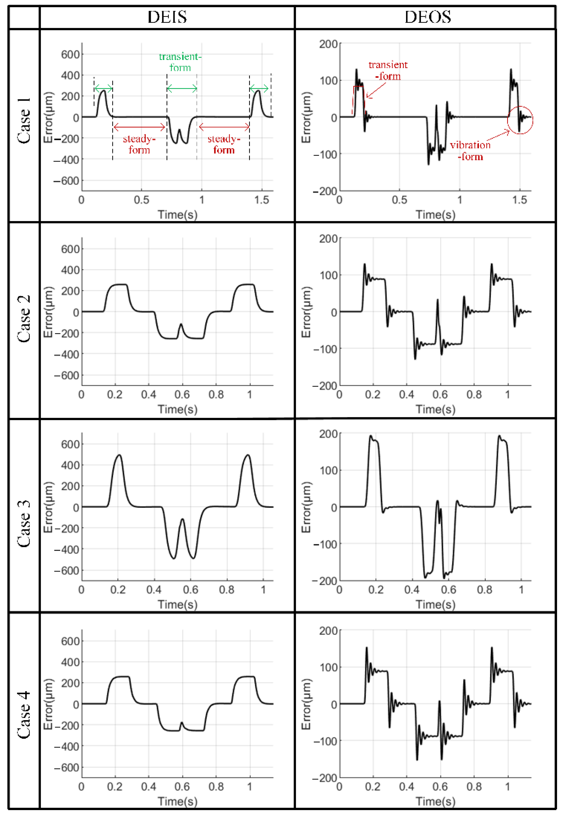
2.2. The DEIS and DEOS

Taking the to and fro motions as examples, four cases with different motion parameters are used to analyze the DEs. The movement displacement is 200 mm. The limitations of the maximum velocity, acceleration, acceleration establishment time and its corresponding jerk of the four cases are listed in

Table 1. The parameters of the to and fro motions of an individual axis.

Case	The Max. Velocity (mm/min)	The Max. Acceleration (g)	The Max. Acceleration Establishment Time (ms)	The Jerk at the First Peak (m/s3)
1	20,000	0.5	20	432.8
2	40,000	0.5	20	432.8
3	40,000	1.0	40	461.4
4	40,000	0.5	10	820.8

.

According to Table 1, G code was written, and the acceleration, acceleration establishment time and other parameters were set in the KEDE GNC61 CNC system [20]. For the CNC system, G237 and G238 of G code can be used to collect the setpoints position sequences interpolated. G237 starts the acquisition, while G238 stops the acquisition. The sampling period of the CNC system was 2 ms.

The setpoints velocity, acceleration and jerk sequences were obtained by the first-order difference of the setpoints position sequence, as shown in Figure 7. It can be seen from the figure that the maximum velocity and the maximum acceleration of each case reached the limitation values. In cases 1, 2, 3 and 4, the jerk at the first peak was 432.8 m/s³, 432.8 m/s³, 461.4 m/s³ and 820.8 m/s³, respectively. At the time point of changing direction, the jerk of each case changed dramatically relative to other time points. This drastic change have resulted from the calculation error caused by the low sampling frequency, which is not considered in the subsequent analysis.

By inputting the setpoints of the four cases listed in Table 1 into the servo control model shown in Figure 4, the DEIS and the DEOS were obtained, as shown in Figure 8.

The servo control model shown in Figure 4 adopts Feedforward Control, which reduces the DEIS caused by phase lag. Therefore, in Figure 8, the steady-form DEIS in the constant velocity segment was nearly zero, while the transient-form DEIS existed in the acceleration and deceleration segment.

In Figure 8, the DEOS takes two forms: transient and vibration. The transient-form DEOS is the elastic deformation of the mechanical structures outside the servo-loop caused by the inertia force. The transient-form DEOS exists in the acceleration and deceleration segment. In the uniform velocity segment, there was no such error.

The vibration-form DEOS was caused by the jerk. The DEOS took the vibration-form at the time point when the jerk was acted. After the jerk was un-acted, the DEOS kept the residual vibration, as shown in Figure 8.

3. Setpoints Time–Frequency Analysis

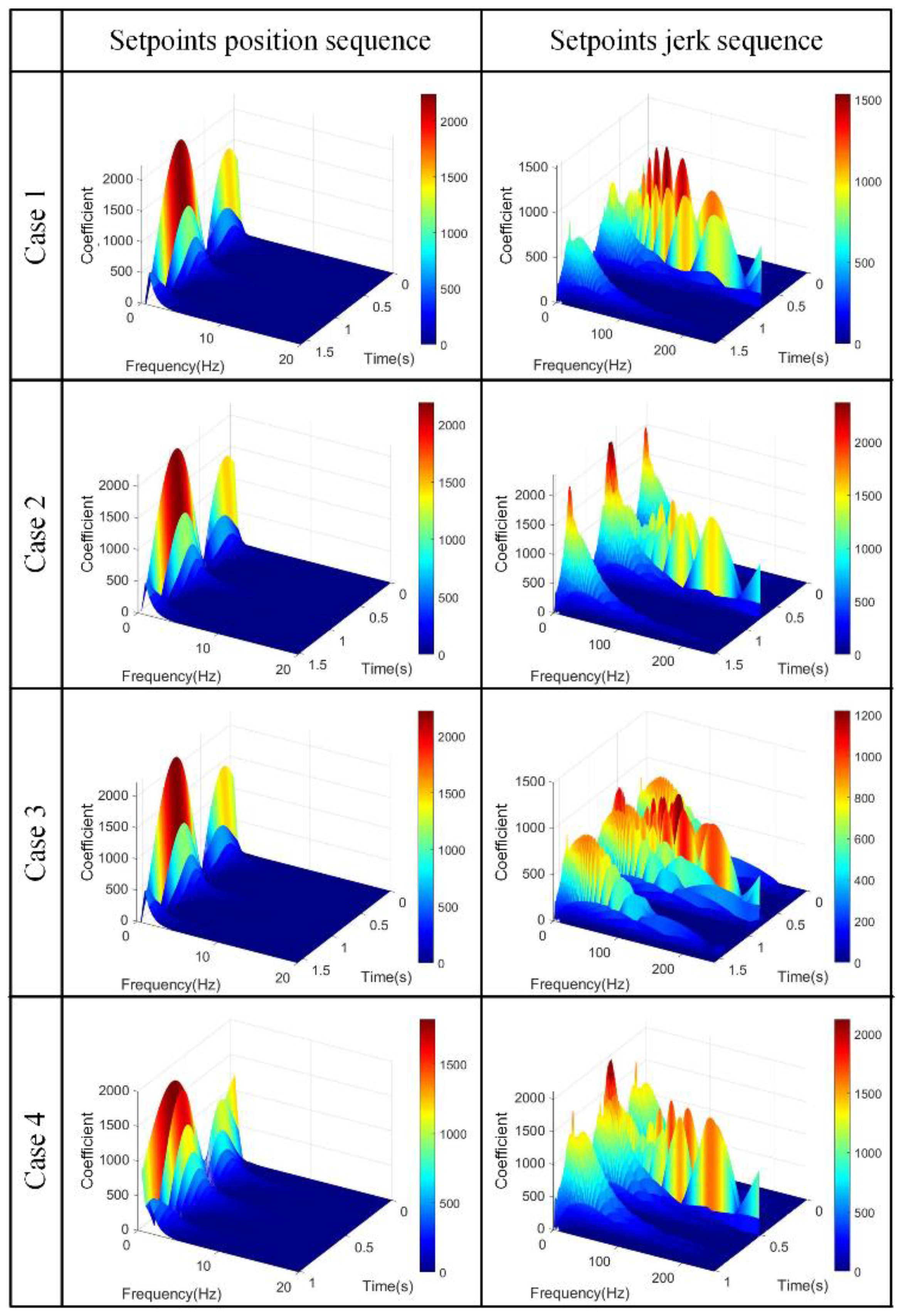
3.1. Construction of the Setpoints Time–Frequency Diagrams

Suppose that the setpoints position sequence input into a servo feed system is as follows:

$$\begin{array}{cc}p\left(i\right)& i=1,2,\dots n\end{array}$$

(13)

where i is the number of sampling points.

By calculating the difference of the setpoints position sequence, the velocity sequence v, the acceleration sequence a and the jerk sequence, j are obtained as follows:

$$\{\begin{array}{c}v=\frac{\mathsf{\Delta }p}{\frac{1}{f_s}}\\ a=\frac{\mathsf{\Delta }v}{\frac{1}{f_s}}\\ j=\frac{\mathsf{\Delta }a}{\frac{1}{f_s}}\end{array}$$

(14)

where Δ is differential symbol and f_s is the sampling period.

The frequency domain representation of setpoints changes over time, so the setpoints are nonstationary signals. The wavelet transform is a time–frequency transform, which is ideal for the analysis of non-stationary signals. In addition, by setting proper scale and translation, the wavelet transform can provide proper time resolution and frequency resolution for analyzing DEs. Therefore, the wavelet transform is applied to the position sequence and the jerk sequence:

$$\{\begin{array}{c}{W}_p\left(u,s\right)={\displaystyle \int }p\frac{1}{\sqrt{s}}{\psi }^{*}\left(\frac{t-u}{s}\right)dt\\ W_j\left(u,s\right)={\displaystyle \int }j\frac{1}{\sqrt{s}}{\psi }^{*}\left(\frac{t-u}{s}\right)dt\end{array}$$

(15)

where $\psi \left(t\right)$ is wavelet base function; s is scale; u is time shift; * is the conjugation operator; $W_p\left(u,s\right)$ and $W_j\left(u,s\right)$ are wavelet coefficients; and t is time.

In order to make the time shift, u, with time, t, the sampling period, f_s, is used to construct the time-shift sequence as follows:

$$u=\left[\begin{array}{ccc}0& \frac{1}{f_s}& \frac{2}{f_s}\end{array}\begin{array}{cc}\cdots & \frac{n-1}{f_s}\end{array}\right]$$

(16)

In order to make the scale, s, with frequency, f, it is necessary to construct the scale sequence as follows:

$$s=\left[\begin{array}{cc}\frac{2f_{c}L}{1}& \begin{array}{ccc}\frac{2f_{c}L}{2}& \cdots & \begin{array}{cc}\frac{2f_{c}L}{L-1}& \frac{2f_{c}L}{L}\end{array}\end{array}\end{array}\right]$$

(17)

where $f_c$ is the center frequency of the wavelet base function and L is the length of the scale sequence.

The pseudo-frequency corresponding to the scale, s, in Hz, f is:

$$f=\frac{f_c}{s\mathrm{\Delta }T}=\frac{f_c{f}_s}{s}$$

(18)

where $\mathrm{\Delta }T$ is the sampling period.

Plugging Equation (16) into Equation (17), the frequency sequence can be obtained as follows:

$$f=\left[\begin{array}{ccccc}\frac{f_s}{2}\frac{1}{L}& \frac{f_s}{2}\frac{2}{L}& \cdots & \frac{f_s}{2}\frac{L-1}{L}& \frac{f_s}{2}\frac{L}{L}\end{array}\right]$$

(19)

According to Equations (13)–(18), a time–frequency diagram with the setpoints frequency as the X-axis, the time as the Y-axis and the wavelet coefficient as the Z-axis can be obtained, which characterizes the variation of setpoints frequency with time.

In Equation (14), there are many wavelet base functions that can be selected, such as Morlet, Db and Symlet, and so on. Different wavelet base functions lead to different time–frequency diagrams. Compared with the wavelet base function of Morlet and Db2, Sym2 is more suitable for setpoints because variations in the setpoint frequency analyzed by Sym2 presents a high correlation with variations in acceleration and jerk (see the next two sections).

It can be seen from Equation (19) that, with an increase in the length of the scale sequence, L, the resolution of the frequency, f, increased, while the calculation load also increased. In the next two sections, L takes 512 for the tradeoff of the resolution and calculation load.

The sampling period, f_s, of the CNC system was 2 ms, so the frequency range which could be analyzed was 0–250 Hz. According to Equations (16) and (19), the resolution of the time shift, u, was 2 ms, while the resolution of the frequency, f, was 0.488 Hz.

The position loop bandwidth of servo feed systems is usually dozens or hundreds of Hertz [2,21,22,23,24,25]. The frequency range of 0–250 Hz can cover the position loop bandwidth, while the resolution of the frequency, f, is far less than the position loop bandwidth. Therefore, the frequency ranges of 0–250 Hz and a resolution of the frequency, f, of 0.488 Hz are suitable for the analysis of setpoints frequency with adequate frequency cover range and adequate frequency resolution. As for the resolution of the time shift, u, 2 ms is generally far less than the tool trajectory cycle time, so it is suitable for the analysis of setpoints frequency with adequate time resolution.

The selection of the parameters of L and f_s means that the setpoints time–frequency diagram has the adequate time resolution, frequency resolution and frequency cover range. It was therefore suitable to use for further analysis in terms of the TDC of DEs of individual axes along the tool trajectory.

According to the Equations (13)–(19), the time–frequency diagrams of the setpoints position sequence and the jerk sequence were drawn, as shown in Figure 9.

The time–frequency diagram of the setpoints position sequence and the jerk sequence contain the same setpoints frequency components, but the amplitudes are different (i.e., different wavelet coefficients). For example, assuming the setpoints position sequence is a finite continuous signal x(t). It can be decomposed into Fourier series as follows:

$$x\left(t\right)=\frac{1}{2}{a}_0+{\displaystyle \sum }_{n=1}^{+\infty }{A}_{n}cos({\omega }_{n}t+{\phi }_n)$$

(20)

where $A_n$ is the amplitude; ${\omega }_n$ is the frequency; and ${\phi }_n$ is the phase angle.

By third order deriving the equation from both sides, the setpoint jerk is obtained as follows:

$$\stackrel{⃛}{x}\left(t\right)={\displaystyle \sum }_{n=1}^{+\infty }{A}_n{\omega }_n{}^{3}cos({\omega }_{n}t+{\phi }_n)$$

(21)

The frequency components of the setpoints position sequence and jerk sequence are same, but the amplitudes are $A_n$ and $A_n{\omega }_n{}^3$, respectively. Compared with the amplitude of the spectrum of the position, the amplitude of high frequency components in the spectrum of jerk are amplified.

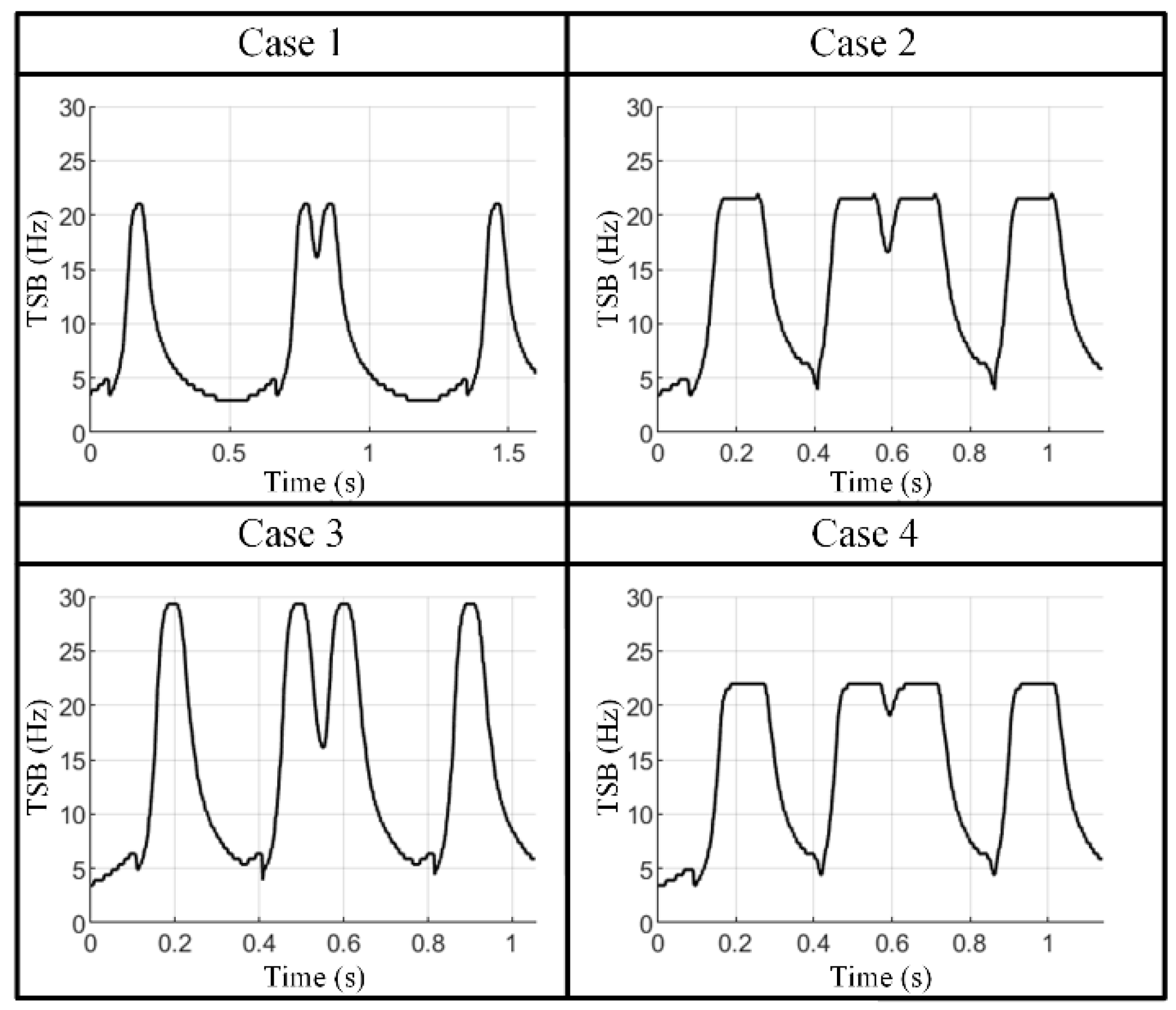
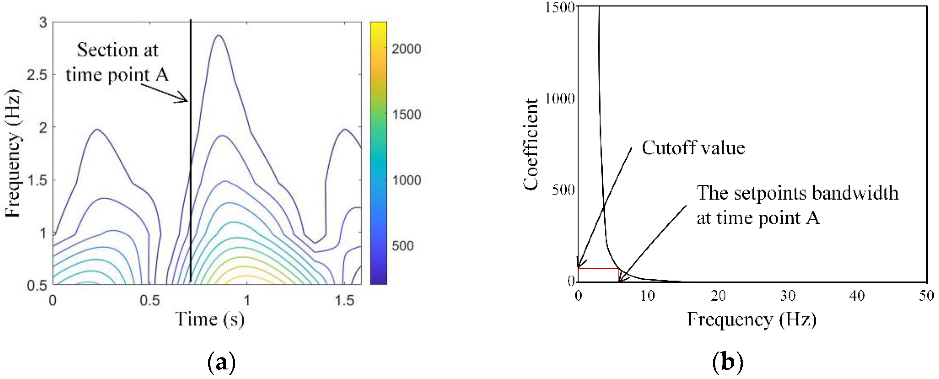
3.2. Extraction of Time-Dependent Setpoint Bandwidth (TDSB)

The DEIS is the deviation of the feedback detection position from the setpoints position. It is caused by the phase lag and amplitude attenuation of the servo feed system against the setpoints [22,24,25,26]. In that sense the setpoints position sequence is the input of the servo feed system in CNC machine tools and has direct effects on the DEIS, the time–frequency diagram constructed by the setpoints position sequence is employed to extract the TDSB for analyzing the TDC of the DEIS.

The time–frequency diagram of the setpoints position sequence reflects the relationship between wavelet coefficient, time and frequency. Figure 10a shows a contour map of a setpoints time–frequency diagram. It can be seen from the figure that at a certain time point, with the increase of frequency, the wavelet coefficient decreased. The smaller the wavelet coefficient, the smaller the similarity between the components of the signal and the wavelet. When the wavelet coefficient is reduced to a certain degree, it is considered that the setpoints no longer contain the frequency component corresponding to the coefficient. Therefore, the setpoint bandwidth at a certain time point is defined as the frequency where the coefficient does not exceed a small value (titled as the cutoff value below) of the maximum coefficient in the time–frequency diagram, as shown in Figure 10b. According to this definition, the setpoint bandwidths along the time points constitute the TDSB.

According to the method described above, the TDSBs of the four cases were drawn, as shown in Figure 11. The setpoint bandwidth was related to the cutoff value. Due to the wavelet coefficient being basically monotone and decreasing, a small value, 0.1%, was set to the cutoff value so that the frequency range was covered. Although the TDSB cannot reflect the absolute value of the setpoint bandwidth, it can reflect the variation in setpoint bandwidth with time qualitatively, which can be used to analyze the TDC of the DEIS, as described in the following sections.

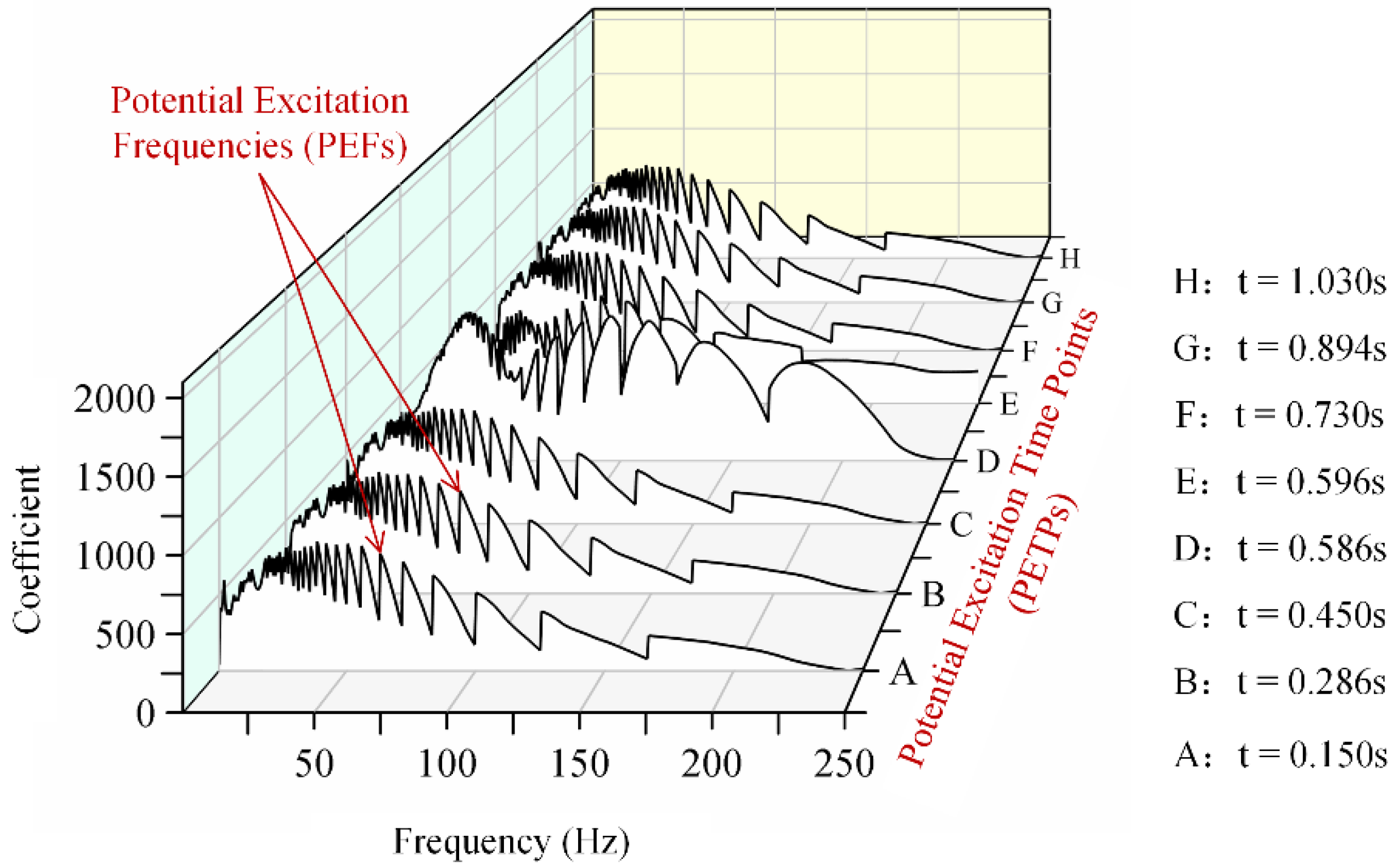
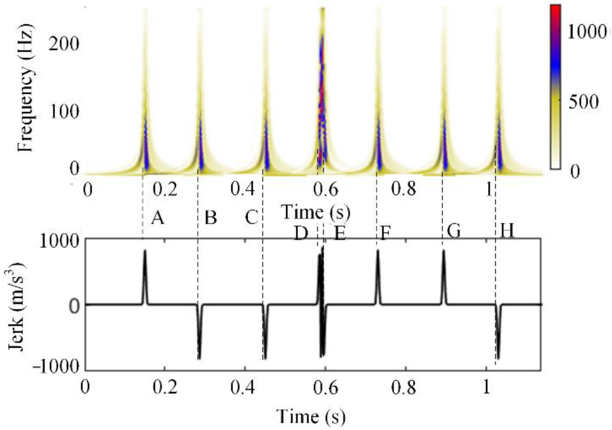
3.3. Extraction of Time-Dependent Potential Excitation (TDPE)

The DEOS is the deviation of the actual position of the effector end from the feedback detection position. It includes two forms: elastic deformation and vibration. The former is the elastic deformation of mechanical structures outside the servo-loop caused by the inertia force/moment generated by the setpoints acceleration [27,28,29,30,31]; the latter is the vibration of mechanical structures outside the servo-loop excited by the jerk of the setpoints [14,32,33,34]. Because the dynamic excitation from setpoints is the cause of the DEOS in vibration-form [35], the time–frequency diagram of the setpoint jerk sequence is used to extract the TDPE for analyzing DEOS in vibration-form.

In the time–frequency diagrams of the setpoint jerk sequence, shown in Figure 9, there are obvious “ridge lines” at several time points, indicating that there are Potential Excitation Time Points (PETPs) in setpoints at the time points at which the Potential Excitation Frequencies (PEFs) are presented. Therefore, the TDPE is presented as the PETPs and PEFs. Figure 12 shows eight “ridge lines” in the time–frequency diagram of the 4th case, whose time points A, B, C, D, E, F, G and H are PETPs. Figure 12 shows the PEFs at the eight PETPs. In the case of these PETPs, if the PEFs contained in the setpoints coincide with the natural frequencies of the mechanical structures outside the servo-loop, the vibrations may be excited.

4. Mechanism Analysis

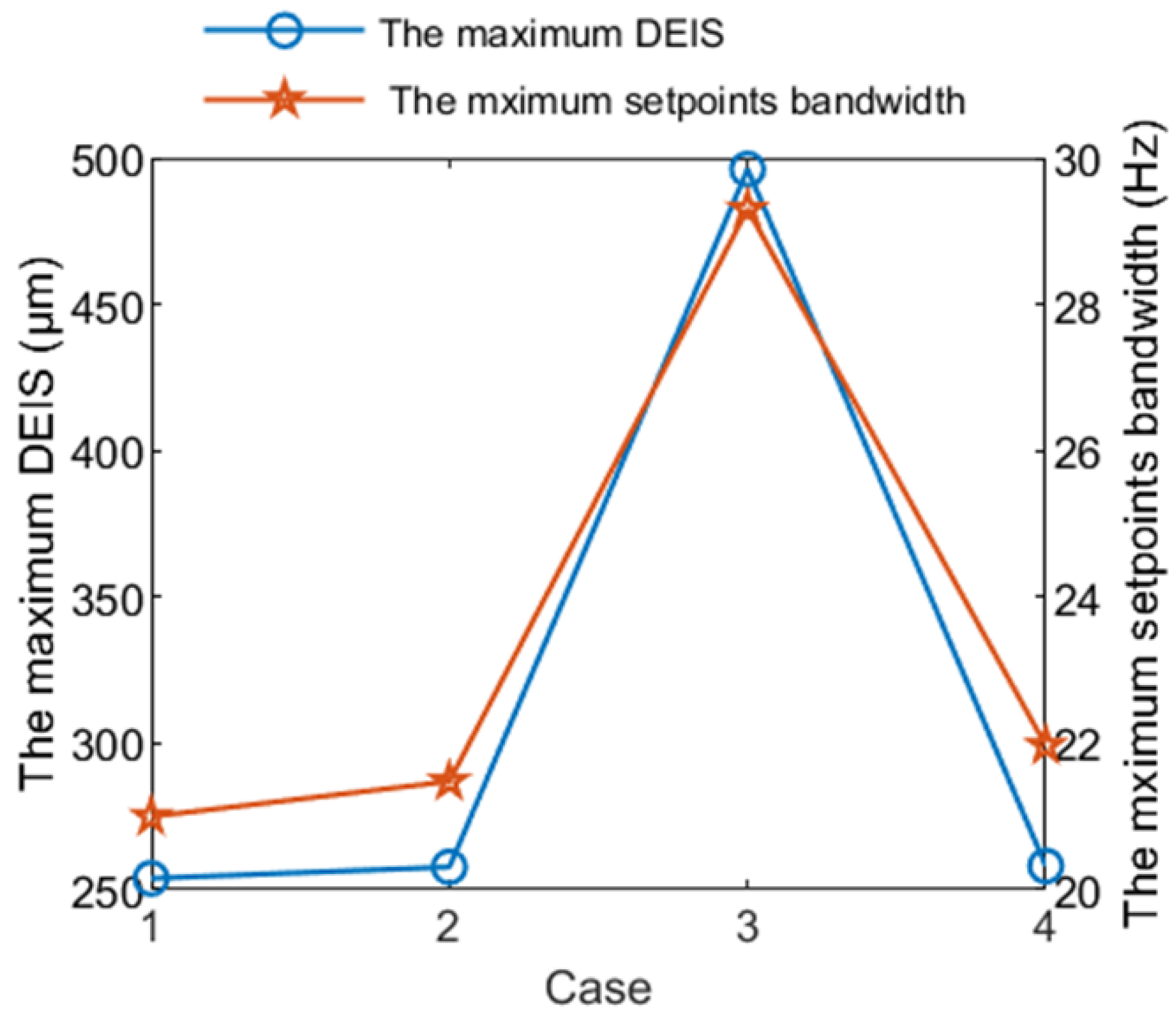
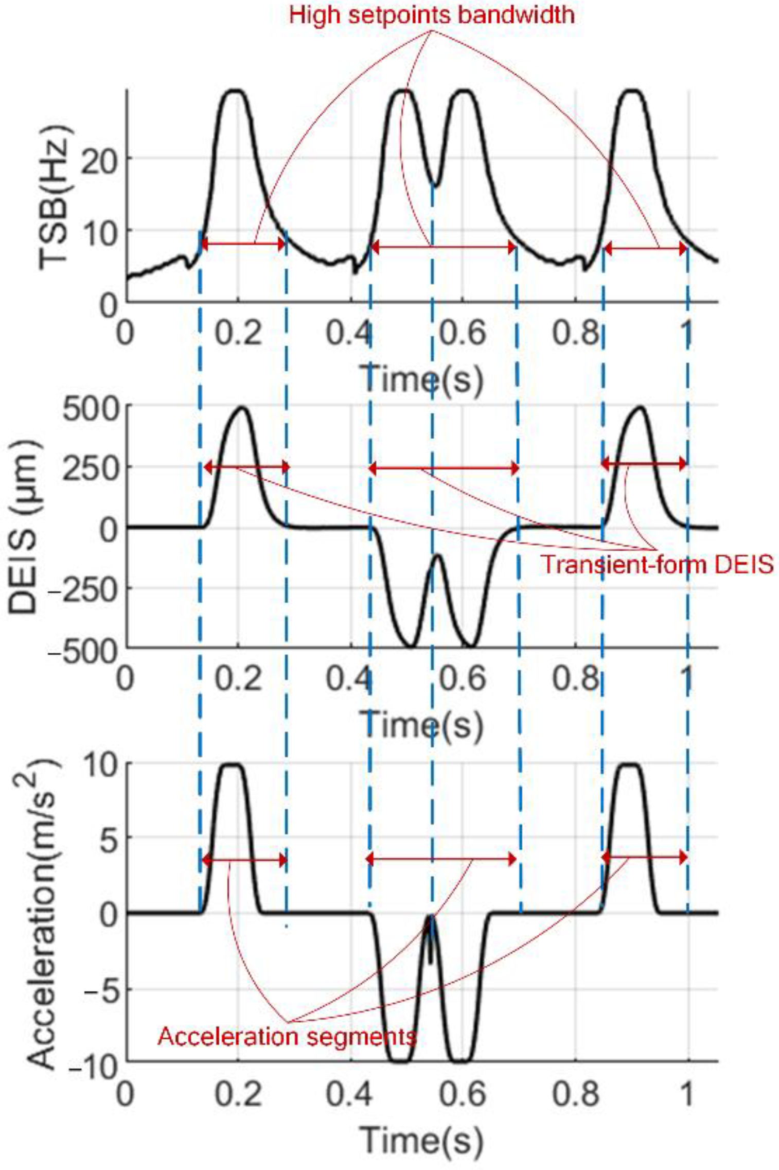
4.1. The Correlation between TDSBs and the DEIS

Figure 13 shows the curves of the TDSB, DEIS and setpoint acceleration with time in the 3rd case. The three curves present an obvious TDC. The change in the trends of the three curves are nearly consistent, which means the TDSB, DEIS and setpoint acceleration have significant correlation. The TDSB corresponding to the large acceleration is very large, while the DEIS corresponding to the large TDSB is also large, and vice versa.

It can be seen from Figure 7 and Figure 11 that the TDSBs are related to the acceleration. The maximum acceleration of the 3rd case was much larger than that of the other three cases. Correspondingly, the maximum setpoint bandwidth of the 3rd case was obviously higher than that of the other cases. In addition, the maximum acceleration of the 1st, 2nd and 4th cases were same, although there were differences in terms maximum velocity and jerk. Correspondingly, the maximum setpoint bandwidth of these three cases were nearly consistent. The analysis mentioned above means that there is a close correlation between the TDSB and setpoint acceleration.

Figure 14 shows the maximum setpoint bandwidth and its corresponding DEIS in the four cases. The setpoint bandwidth is closely related to the DEIS. The larger the setpoint bandwidth, the larger the DEIS. The maximum setpoint bandwidths of the 1st, 2nd, and 4th cases were about 21 Hz, and that of the 3rd case was about 29 Hz. Accordingly, the maximum DEISs of the cases with lower setpoint bandwidths were about 250 μm, while that with a lager setpoint bandwidth was about 495 μm. Moreover, the setpoint bandwidth was dominated by the setpoint acceleration. The 3rd case had a higher acceleration, 1 g, than the other three cases, 0.5 g, so it has the highest setpoint bandwidth and the largest DEIS. It can be seen from the figure that the DEIS has a direct correlation with the setpoint bandwidth.

To sum up, the TDSB induced by the change in setpoint acceleration is the main cause of the TDC of the DEIS. The change in setpoint acceleration results in the TDSB, and further results in the TDC of the DEIS. At a time point, a larger setpoint acceleration leads to a larger setpoint bandwidth, and hence the large DEIS.

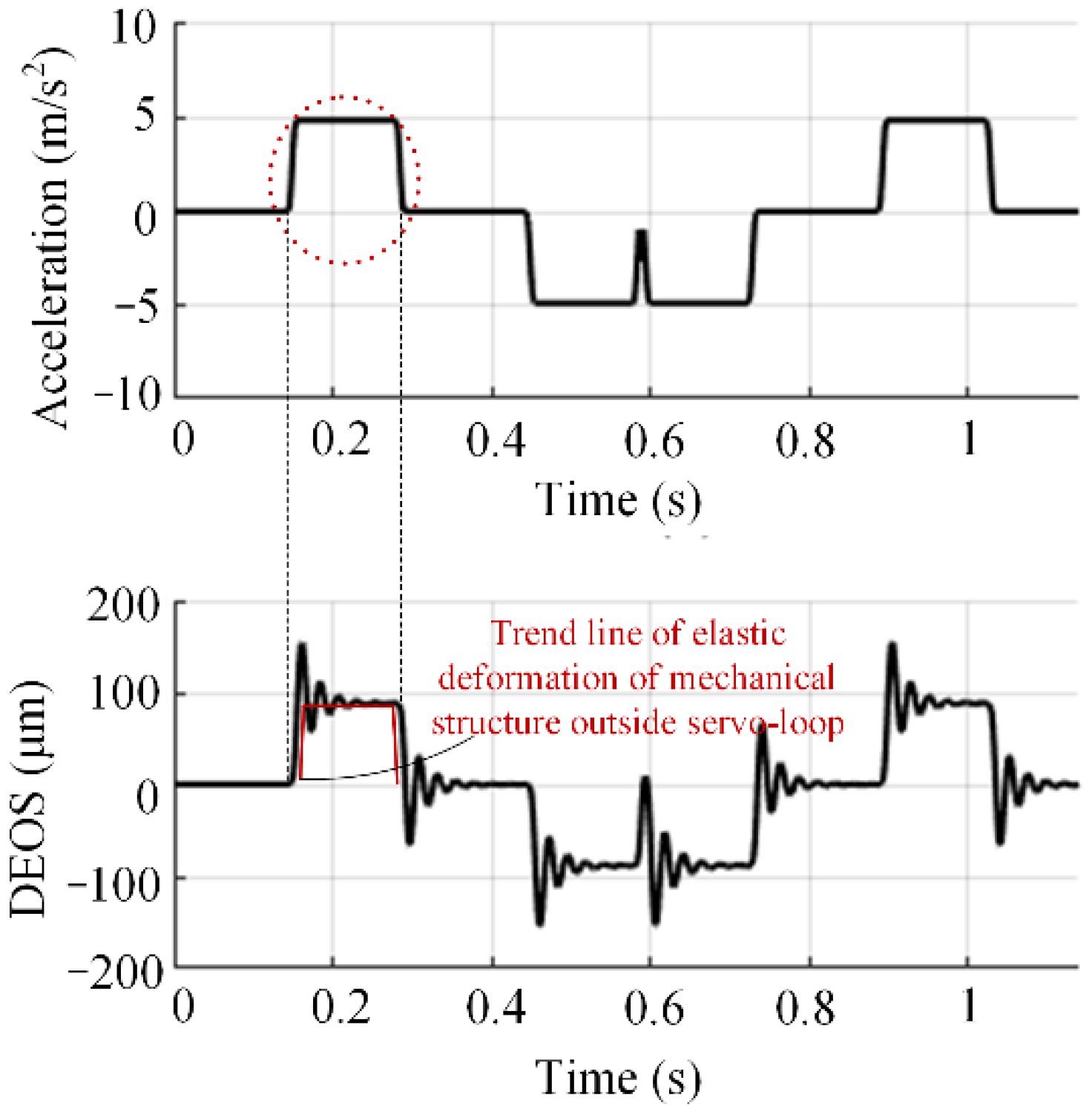
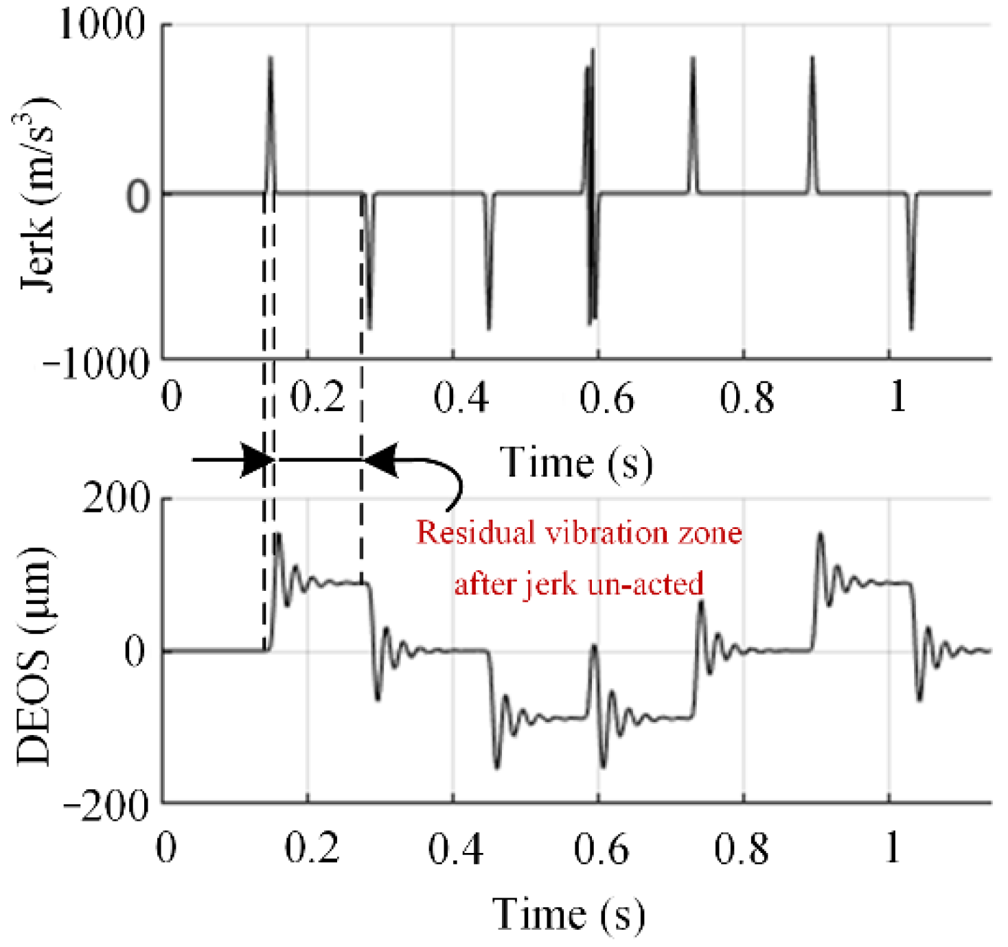
4.2. The Correlation between TDPEs and the DEOS

Figure 15 shows the curve of the DEOS and setpoint acceleration with time of the 4th case. The elastic deformation (transient-form DEOS) trend line, which corresponds to acceleration, is shown in the figure. It is noted that, in the whole-time axis of Figure 15, the transient-form DEOS is consistent with the acceleration curve. Therefore, the setpoint acceleration accounts for the transient-form DEOS.

The same results can be found in Figure 7 and Figure 8. It can be seen from these figures that the maximum acceleration of the 3rd case was much larger than that of the other three cases. Correspondingly, the maximum transient-form DEOS of the 3rd case was obviously higher than those of the other cases. The maximum setpoint acceleration of the 1st, 2nd, and 4th cases were 0.5 g, and that of the 3rd case was 1 g. The transient-form DEOS of the latter (about 180 μm) was twice as much as the former (about 90 μm). Moreover, the maximum acceleration of the 1st, 2nd and 4th cases were same, although there were differences in maximum velocity and jerk. Correspondingly, the maximum transient-form DEOS of these three cases were nearly consistent.

The analysis mentioned above means that the change in setpoint acceleration accounts for the TDC of transient-form DEOS.

Figure 16 shows the curve of the DEOS and the setpoint jerk in the 4th case. It can be seen from the figure that when the jerk was acted, the DEOS presented the vibration-form DEOS. After the jerk was un-acted, the vibration-form DEOS kept the residual vibration.

The time–frequency diagrams of the setpoint jerk sequence, as shown in Figure 9 and Figure 12, include obvious “ridge lines” (PETPs). By contour map, the upper half in Figure 17 shows these “ridge lines” of the 4th case in time–frequency domain. Meanwhile, the lower half in Figure 17 shows the setpoint jerk sequence in time-domain.

It can be seen from the Figure 16 and Figure 17 that the PETPs exactly correspond to the times at the peak of the jerks in the time-domain. It also accounts for the initial points of the vibration-form DEOS.

FFT analysis was undertaken for the vibration-form DEOS, as shown in the lower half of Figure 18. Meanwhile, the upper half of Figure 18 shows the “ridge line” section at the PETP A. It can be seen from the figure that the main frequency of the residual vibration (vibration-form DEOS) is 45.9 Hz. In the PEFs at the PETP A, the frequency component of 45.9 Hz is also included. It is noted that the main frequency of residual vibration was near to, but did not coincide with, the natural frequency of 53.2 Hz of the servo feed system, as shown in Figure 3. The noncoincidence between the two frequencies was caused by the low frequency resolution of the residual vibration frequency spectrum. There were no other natural frequencies around 53.2 Hz in the model of the servo feed system. It is therefore reasonable to believe that the residual vibration is excited by the setpoints PEF.

Figure 19 compares the “ridge line” at time point A for the four cases. In these four cases, the maximum jerk of the 4th case was much larger than that of the other three cases. Correspondingly, the PEF amplitude of the 4th case was obviously higher than that of the other cases. In addition, the maximum jerks of the 1st, 2nd and 3rd cases were nearly the same, although there were differences in maximum velocity and acceleration. Correspondingly, there was only a slight difference in PEF amplitude in these three cases.

It can be concluded from the analysis mentioned above that the change in setpoint jerk accounts for the time-dependent characteristic of the vibration-form DEOS. The time points of the jerk peaks correlate to the PETPs. This determines the initial points of the vibration-form DEOS. In addition, the setpoint jerk responds to the PEF at a PETP. A large setpoint jerk results in a larger amplitude and the wider distribution of PEF.

5. Conclusions

In this study, the TDCs of DEs are presented by inputting the setpoints of to and fro motions into the servo dynamics model. Meanwhile, the TDCs of setpoints is extracted by time–frequency analysis. On these bases, the correlations between the TDC of setpoint frequency and the TDCs of DEs are analyzed. Thanks to this analysis, the mechanism of the TDC of DE can be summarized as follows:

The TDSB, which is related to setpoint acceleration, accounts for the TDC of the DEIS. When the maximum setpoint acceleration increases from 0.5 g to 1 g, the maximum setpoint bandwidth increases from about 21 Hz to 29 Hz, and the maximum DEIS increases from about 250 μm to 495 μm.

The TDPE, which is related to the setpoint jerk, accounts for the TDC of the DEOS in vibration-form. The PETP determines the time points when the vibration may be excited, while the PEF determines the frequency by which it is possible to excite the vibration. The PEF amplitude increases with an increase in the maximum jerk.

The TDC of the transient-form DEOS is determined by the change in setpoint acceleration. When the setpoint acceleration increases from 0.5 g to 1 g, the transient-form DEOS increases from about 90 μm to 180 μm.

References

1. Lyu, D.; Liu, Q.; Liu, H.; Zhao, W. Dynamic error of CNC machine tools: A state-of-the-art review. Int. J. Adv. Manuf. Technol. 2020, 106, 1869–1891. [Google Scholar] [CrossRef]
2. Altintas, Y.; Verl, A.; Brecher, C.; Uriarte, L.; Pritschow, G. Machine tool feed drives. CIRP Ann. Manuf. Technol. 2011, 60, 779–796. [Google Scholar] [CrossRef]
3. Huo, F.; Poo, A.-N. Precision contouring control of machine tools. Int. J. Adv. Manuf. Technol. 2013, 64, 319–333. [Google Scholar] [CrossRef]
4. Tang, L.; Landers, R.G. Multiaxis Contour Control—the State of the Art. IEEE Trans. Control. Syst. Technol. 2013, 21, 1997–2010. [Google Scholar] [CrossRef]
5. Uriarte, L.; Zatarain, M.; Axinte, D.; Yagüe-Fabra, J.; Ihlenfeldt, S.; Eguia, J.; Olarra, A. Machine tools for large parts. CIRP Ann. 2013, 62, 731–750. [Google Scholar] [CrossRef]
6. Oomen, T. Advanced Motion Control for Precision Mechatronics: Control, Identification, and Learning of Complex Systems. IEEJ J. Ind. Appl. 2018, 7, 127–140. [Google Scholar] [CrossRef] [Green Version]
7. Yuan, M.; Manzie, C.; Good, M.; Shames, I.; Gan, L.; Keynejad, F.; Robinette, T. A review of industrial tracking control algorithms. Control. Eng. Pract. 2020, 102, 104536. [Google Scholar] [CrossRef]
8. Tajima, S.; Sencer, B. Global tool-path smoothing for CNC machine tools with uninterrupted acceleration. Int. J. Mach. Tools Manuf. 2017, 121, 81–95. [Google Scholar] [CrossRef]
9. Jia, Z.-Y.; Song, D.-N.; Ma, J.-W.; Hu, G.-Q.; Su, W.-W. A NURBS interpolator with constant speed at feedrate-sensitive regions under drive and contour-error constraints. Int. J. Mach. Tools Manuf. 2017, 116, 1–17. [Google Scholar] [CrossRef]
10. Erkorkmaz, K.; Chen, Q.-G.; Zhao, M.-Y.; Beudaert, X.; Gao, X.-S. Linear programming and windowing based feedrate optimization for spline toolpaths. CIRP Ann. 2017, 66, 393–396. [Google Scholar] [CrossRef]
11. Wang, Y.S.; Yang, D.S.; Gai, R.L.; Wang, S.H.; Sun, S.J. Design of trigonometric velocity scheduling algorithm based on pre-interpolation and look-ahead interpolation. Int. J. Mach. Tools Manuf. 2015, 96, 94–105. [Google Scholar] [CrossRef]
12. Tulsyan, S.; Altintas, Y. Local toolpath smoothing for five-axis machine tools. Int. J. Mach. Tools Manuf. 2015, 96, 15–26. [Google Scholar] [CrossRef]
13. Sencer, B.; Ishizaki, K.; Shamoto, E. A curvature optimal sharp corner smoothing algorithm for high-speed feed motion generation of NC systems along linear tool paths. Int. J. Adv. Manuf. Technol. 2015, 76, 1977–1992. [Google Scholar] [CrossRef]
14. Nam, S.-H.; Yang, M.-Y. A study on a generalized parametric interpolator with real-time jerk-limited acceleration. Comput. Aided Des. 2004, 36, 27–36. [Google Scholar] [CrossRef]
15. Smith., D.A. Wide Bandwidth Control of High-Speed Milling Machine Feed Drives; University of Florida: Gainesville, FL, USA, 1999. [Google Scholar]
16. Rotariu, I.; Ellenbroek, R.; Steinbuch, M. Time-Frequency Analysis of a Motion System with Learning Control. In Proceedings of the American Control Conference, Denver, CO, USA, 4–6 June 2003. [Google Scholar]
17. Hennen, B.; Rotariu, I.; Steinbuch, M. Time-frequency analysis of position-dependent dynamics in a Motion System with ILC. In Proceedings of the American Control Conference, ACC ‘07, New York, NY, USA, 11–13 July 2007. [Google Scholar]
18. Rotariu, I.; Steinbuch, M.; Ellenbroek, R. Adaptive iterative learning control for high precision motion systems. IEEE Trans. Control. Syst. Technol. 2008, 16, 1075–1082. [Google Scholar] [CrossRef]
19. Alkafafi, L. Time and Frequency Optimal Motion Control of CNC Machine Tools; Technische Universität Hamburg: Hamburg, Germany, 2013. [Google Scholar]
20. GNC62. Available online: https://www.dlkede.com/plus/view.php?aid=11 (accessed on 13 January 2022).
21. Erkorkmaz, K.; Kamalzadeh, A. Compensation of axial vibrations in ball screw drives. CIRP Ann. Manuf. Technol. 2007, 56, 373–378. [Google Scholar]
22. Okwudire, C.; Altintas, Y. Minimum tracking error control of flexible ball screw drives using a discrete-time sliding mode controller. ASME Trans. J. Dyn. Syst. Meas. Control. 2009, 131, 051006. [Google Scholar] [CrossRef]
23. Sun, Z.; Zahn, P.; Verl, A.; Lechler, A. A new control principle to increase the bandwidth of feed drives with large inertia ratio. Int. J. Adv. Manuf. Technol. 2017, 91, 1747–1752. [Google Scholar] [CrossRef]
24. Sencer, B.; Dumanli, A. Optimal control of flexible drives with load side feedback. CIRP Ann. Manuf. Technol. 2017, 66, 357–360. [Google Scholar] [CrossRef]
25. Liu, H.; Zhang, J.; Zhao, W. An Intelligent Non-Collocated Control Strategy for Ball-Screw Feed Drives with Dynamic Variations. Engineering 2017, 3, 641–647. [Google Scholar] [CrossRef]
26. Erkorkmaz, K.; Kamalzadeh, A. High bandwidth control of ball screw drives. CIRP Ann. Manuf. Technol. 2006, 55, 393–398. [Google Scholar] [CrossRef]
27. Bringmann, B.; Maglie, P. A method for direct evaluation of the dynamic 3D path accuracy of NC machine tools. CIRP Ann. Manuf. Technol. 2009, 58, 343–346. [Google Scholar] [CrossRef]
28. Knapp, W.; Weikert, S. Testing the Contouring Performance in 6 Degrees of Freedom. Ann. CIRP 1999, 48, 433–436. [Google Scholar] [CrossRef]
29. Matsubara, A.; Nagaoka, K.; Fujita, T. Model-reference feedforward controller design for high-accuracy contouring control of machine tool axes. CIRP Ann. 2011, 60, 415–418. [Google Scholar] [CrossRef]
30. Denkena, B.; Overmeyer, L.; Litwinski, K.M.; Peters, R. Compensation of geometrical deviations via model based-observers. Int. J. Adv. Manuf. Technol. 2014, 73, 989–998. [Google Scholar] [CrossRef]
31. Steinlin, M.; Weikert, S.; Wegener, K. Open loop inertial cross-talk compensation based on measurement data. In Proceedings of the 25th Annual Meeting of the American Society for Precision Engineering, ASPE 2010, Atlanta, GA, USA, 31 October–4 November 2010; pp. 101–104. [Google Scholar]
32. Ansoategui, I.; Campa, F.J.; López, C.; Díez, M. Influence of the machine tool compliance on the dynamic performance of the servo drives. Int. J. Adv. Manuf. Technol. 2017, 90, 2849–2861. [Google Scholar] [CrossRef]
33. Dong, J.; Ferreira, P.M.; Stori, J.A. Feed-rate optimization with jerk constraints for generating minimum-time trajectories. Int. J. Mach. Tools Manuf. 2007, 47, 1941–1955. [Google Scholar] [CrossRef]
34. Erkorkmaz, K.; Altintas, Y. High speed CNC system design. Part I: Jerk limited trajectory generation and quintic spline interpolation. Int. J. Mach. Tools Manuf. 2001, 41, 1323–1345. [Google Scholar] [CrossRef]
35. Barre, P.-J.; Bearee, R.; Borne, P.; Dumetz, E. Influence of a Jerk Controlled Movement Law on the Vibratory Behaviour of High-Dynamics Systems. J. Intell. Robot. Syst. 2005, 42, 275–293. [Google Scholar] [CrossRef]
Figure 1. The causes of deviation of actual trajectory relative to tool trajectory.
Machines 10 00160 g001
Figure 2. Equivalent dynamics model of ball screw feed system of X-axis cascaded with Z-axis.
Machines 10 00160 g002
Figure 3. Drive point FRF from motor torque to angular velocity of screw shaft at encoder.
Machines 10 00160 g003
Figure 4. Control block diagram of servo feed system.
Machines 10 00160 g004
Figure 5. Comparison of the simulated and experimental drive point FRFs.
Machines 10 00160 g005
Figure 6. Experimental results of the three low order modals: (a) The first order vibration mode (23 Hz); (b) the second order vibration mode (49.8 Hz); and (c) the third order vibration mode (68 Hz).
Machines 10 00160 g006
Figure 7. Setpoints velocity, acceleration and jerk of the four cases.
Machines 10 00160 g007
Figure 8. The DEIS and DEOS of the four cases.
Machines 10 00160 g008
Figure 9. Time–frequency diagrams of setpoints of the four cases.
Machines 10 00160 g009
Figure 10. Definition of cutoff value and setpoint bandwidth at a time point: (a) A contour map of a setpoint time–frequency diagram; (b) the cross-sectional view of the contour map at time point A.
Machines 10 00160 g010
Figure 11. Time-dependent Setpoint Bandwidths (TDSBs) of the four cases.
Machines 10 00160 g011
Figure 12. Time-dependent Potential Excitation (TDPE) of the 4th case.
Machines 10 00160 g012
Figure 13. TDSB, DEIS and setpoint acceleration of the 3rd case.
Machines 10 00160 g013
Figure 14. The relationship between the maximum setpoint bandwidth and the corresponding DEIS.
Machines 10 00160 g014
Figure 15. Setpoint acceleration and DEOS of the 4th case.
Machines 10 00160 g015
Figure 16. Setpoint jerk and DEOS of the 4th case.
Machines 10 00160 g016
Figure 17. PETPs and setpoint jerk of the 4th case.
Machines 10 00160 g017
Figure 18. Comparison of the setpoint frequency and the vibration-form DEOS frequency of the 4th case.
Machines 10 00160 g018
Figure 19. PEFs at PETP A of the four cases.
Machines 10 00160 g019