Predicting the Electrical Impedance of Rolling Bearings Using Machine Learning Methods

Abstract

The present paper describes a measurement setup and a related prediction of the electrical impedance of rolling bearings using machine learning algorithms. The impedance of the rolling bearing is expected to be key in determining the state of health of the bearing, which is an essential component in almost all machines. In previous publications, the determination of the impedance of rolling bearings has already been advanced using analytical methods. Despite the improvements in accuracy achieved within the calculations, there are still discrepancies between the calculated and the measured impedance, leading to an approximately constant off-set value. This discrepancy motivates the machine learning approach introduced in this paper. It is shown that with the help of the data-driven methods the difference between analytical prediction and measurement is reduced to the order of up to 2% across the operational range analyzed so far. To introduce the context of the research shown, first the underlying physics of bearing impedance is presented. Subsequently different machine learning approaches are highlighted and compared with each other in terms of their prediction quality in the results part of this paper. As a further aspect, in addition to the prediction of the bearing impedance, it is investigated whether the rotational speed present at the bearing can be predicted from the frequency spectrum of the impedance using order analysis methods which is independent from the force prediction accuracy. The background to this is that, if the prediction quality is sufficiently high, the additional use of speed sensors could be omitted in future investigations.

1. Introduction

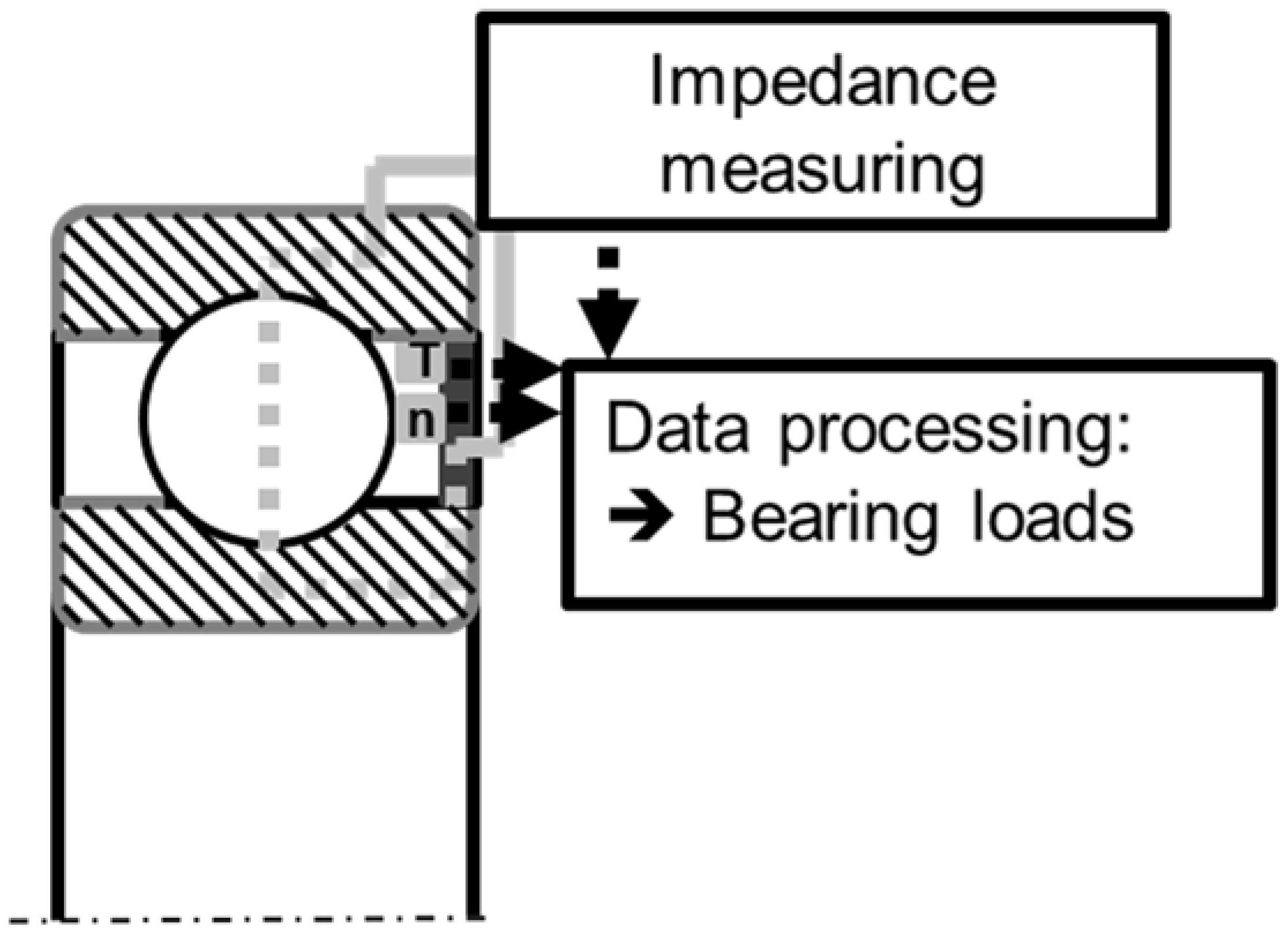
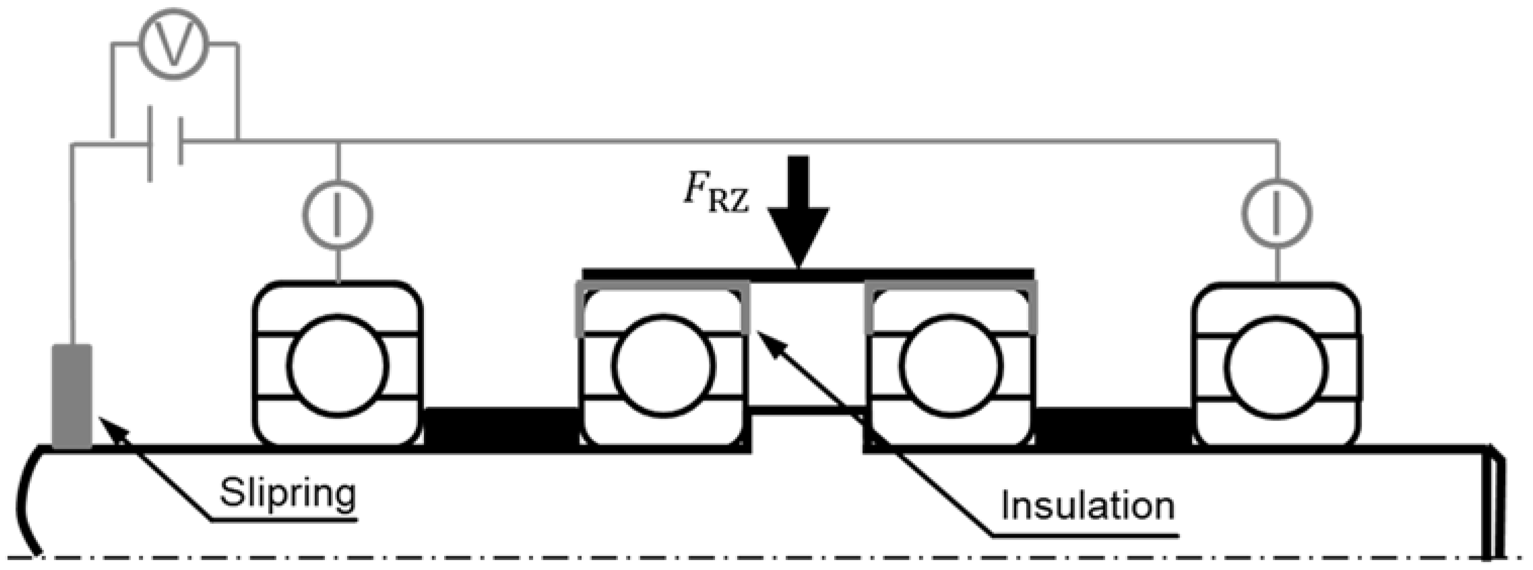
The increasing digitalization in mechanical engineering leads to a demand for new, integrated sensor solutions. Martin et al. [1] have presented a sensor concept, shown in Figure 1, in which the electrical impedance of rolling bearings is measured to estimate the bearing load. With the use of the sensing bearing concept it is possible to implement predictive maintenance and process monitoring more easily in new and existing machines based on load data. The technology is based on the relationship that elasto-hydrodynamic lubricated contacts have a capacitive behavior, which leads to a measurable electrical impedance in an alternating current circuit [2]. The voltage levels of the sensor concept are below harmful values as mentioned in [3]. The literature gives analytical models to describe this effect, but they have an accuracy that is not sufficient to use the models as sensors. For this reason, the models available in the literature were extended in Schirra et al. [3] so that a much more accurate analytical calculation of the bearing impedance is possible. Despite the improvements in the models achieved, there is still a discrepancy between calculated and measured values.

The aim in the application is therefore to determine bearing forces on the basis of the rotational speed, the temperature and the electrical impedance of the rolling bearing. However, in the experiment, the electrical impedance of the rolling bearing cannot be controlled directly, so the bearing load, rotational speed and temperature are the input parameters of the experiment and the data drive methods where the electrical impedance is evaluated. In addition, this makes it easier to compare the results with the literature, which also evaluates the electrical properties. It is also an obvious step to choose the frequency spectrum of the electrical impedance as input parameter, where Martin et al. [1] measured a correlation to the bearing frequencies to replace the input parameter rotational speed. Although the procedure in the experiment is such that the electrical impedance is determined from the bearing load, temperature and rotational speed, the model is used in reverse in the application. The frequency spectrum is thus available in the application and offers the possibility to replace the input parameter rotational speed by the dependencies to the bearing frequencies.

The aim of this paper is to implement the determination of the bearing impedance using machine learning algorithms. It is expected that this method can further reduce the deviation between model and measurement, which are described in the current literature [3].

In the following sections first an overview of the electrical properties of rolling bearings will be given. Thereupon, machine learning methods which are suitable for the regression of the bearing impedance will be presented.

1.1. Electrical Properties of Rolling Bearing Contacts

The electric behavior of rolling bearings was so far mainly analyzed in connection with inverter induced damage phenomena caused by electric discharge (Gemeinder et al. [2], Furtmann et al. [4]), being motivated by the analysis of the contact zone of the loaded rolling elements, current research was often motivated by the increased usage of electric drive systems in individual transport. 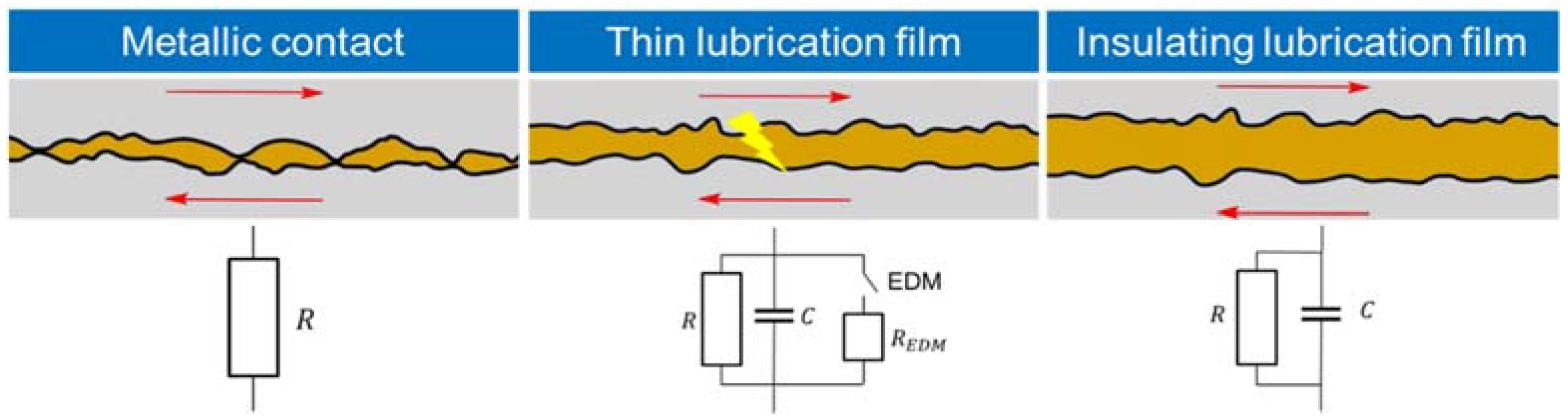Recently the model has been expanded for the hydrodynamic regime [3,4,5] by including the remaining unloaded rolling elements in the analysis. In the boundary friction regime the rolling element behaves like an ohmic resistor whereas the model of a capacitor is appropriate for the hydrodynamic regime, see Figure 2. The rolling element with the highest load or the smallest operational lubrication film thickness, respectively, determines the overall behavior of the rolling bearing.

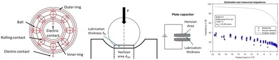
The loaded contact is described using the notion of a plate capacitor with the Hertzian contact area ${\mathit{A}}_{\mathrm{Hz}}$ and the operational lubricant film thickness ${\mathit{h}}_0$ as shown in Figure 3. According to common literature the lubricant is assumed to be an isolator with the specific permittivity ${\mathit{\epsilon }}_{\mathrm{r}}$. The nominal capacity ${\mathit{C}}_{\mathrm{Hz}}$ is calculated by:

$${\mathit{C}}_{\mathrm{Hz}}={\mathit{\epsilon }}_{\mathrm{r}}\times {\mathit{\epsilon }}_0\times \frac{{\mathit{A}}_{\mathrm{Hz}}}{{\mathit{h}}_0}.$$

(1)

Usually, a correction factor $\mathit{k}$ is introduced to account for the effects of the inlet and outlet flow zone as well as for the boundary of the Hertzian contact zone shown in Figure 3 left. Hence, the operational capacity $\mathit{C}$ of the rolling contact in hydrodynamic lubrication conditions is:

$$\mathit{C}={\mathit{C}}_{\mathit{H}\mathit{z}}\times \mathit{k}=\mathit{k}\times {\mathit{\epsilon }}_{{r}}\times {\mathit{\epsilon }}_0\times \frac{{\mathit{A}}_{\mathit{H}\mathit{z}}}{{\mathit{h}}_0}.$$

(2)

The dimensioning of the correction parameter $\mathit{k}$ varies between $\mathit{k}=1,1$ (Gemeinder et al. [4]) and $\mathit{k}=3,5$ (Furtmann et al. [2]). The cage of the rolling bearing can be considered as an insulator or conductor since the influence on the total bearing impedance is within the range of 2%, according to Furtmann. Hence, the overall electric behavior of a rolling bearing in hydrodynamic lubrication can be represented as a network of capacitors as shown in Figure 3, right.

At low speeds or very high loads, respectively, the electric behavior of the rolling bearing tribological system in mixed lubrication conditions changes towards an ohmic resistor, the behavior is of similar type as in (1) and the dependency reads as:

$$\mathit{R}\propto \frac{1}{{\mathit{A}}_{\mathrm{Hz}}}.$$

(3)

When summarizing the electric behavior of the contact in the loaded tribological system by including both the hydrodynamic state represented by Equation (2) as well as the boundary friction state represented by Equation (3) for an alternating current loading condition with frequency $\mathit{f}$ one arrives at the complex impedance of the rolling contact:

$$\mathit{Z}=\mathit{R}+\frac{1}{\mathit{i}\times \mathit{C}}.$$

(4)

The imaginary unit is indicated by the symbol $\mathit{i}$. When measuring with an alternating current of frequency $\mathit{f}$ the transition from mixed, resistive dominated friction to hydrodynamic, capacitive friction should be detectable by a change of the phase angle according to Equation (4) and of the magnitude. When applying a direct current in the measuring circuit the change to occur is from ohmic behavior to an insulating behavior indicated by a change of the impedance of several orders of magnitude.

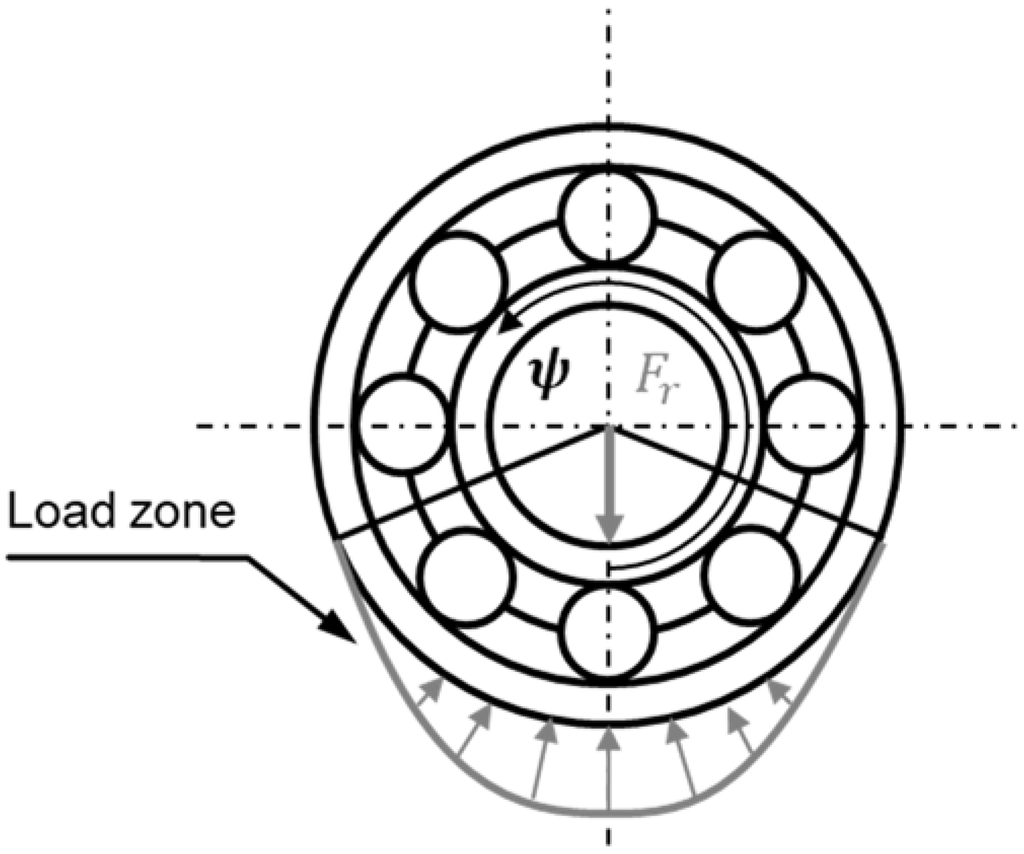
Given the different load conditions (Hamrock & Dowson [7]) the rolling elements are exposed to while traveling through the load zone ${\mathit{Q}}_{\mathit{\psi }}$, the lubrication film governing the overall electric behavior of the rolling bearing is located at the inner race underneath the applied load, as it is shown in Figure 4. This tribological contact is the last one to change its state of operation from mixed to hydrodynamic lubrication since the high load leads to the smallest lubrication film thickness over all contacts, which is why it has a strong impact on the total impedance. Hence, this change from resistive to capacitive behavior needs to be monitored.

So far, the discussion in this section assumes loaded rolling contacts. In rolling bearings, especially when loaded by radial loads only, the unloaded rolling elements outside the load zone $\mathit{\psi }$ sketched in Figure 4 contribute to the overall bearing impedance. Therefore, additional aspects were recently added by Schirra et al. in [3] to the analyses performed by Jablonka et al. in [5] who analyzed a single rolling contact. The additional contributions to the total bearing impedance have significantly helped to reduce the differences between measured and calculated impedance. Remarkably is that, even though no fitting parameter can be used to tune the enhanced model, the difference between model and measurement assumes a more or less constant value which indicates a possible systematic measurement peculiarity which can be easily identified by methods of artificial intelligence.

1.2. Machine Learning Methods

With the increasing amount of available data in all scientific disciplines, the interest in methods that extract information from these data is also growing. This can be observed in the scientific environment as well as in the free market [9]. Hence there is a hypothesis that machine learning can outperform the not sufficient accurate analytical equations in the field of bearing impedance. This machine learning approach has not been studied so far in the scientific environment.

The potential of machine learning methods is enabled by larger data streams made possible by technological advances in hardware, computing power, data storage and data transfer. Likewise, the technologies mentioned are becoming more and more economical. In addition, algorithms are becoming more and more powerful and software less expensive. This is based on the current open source trend since investments primarily come from data-driven industries [9].

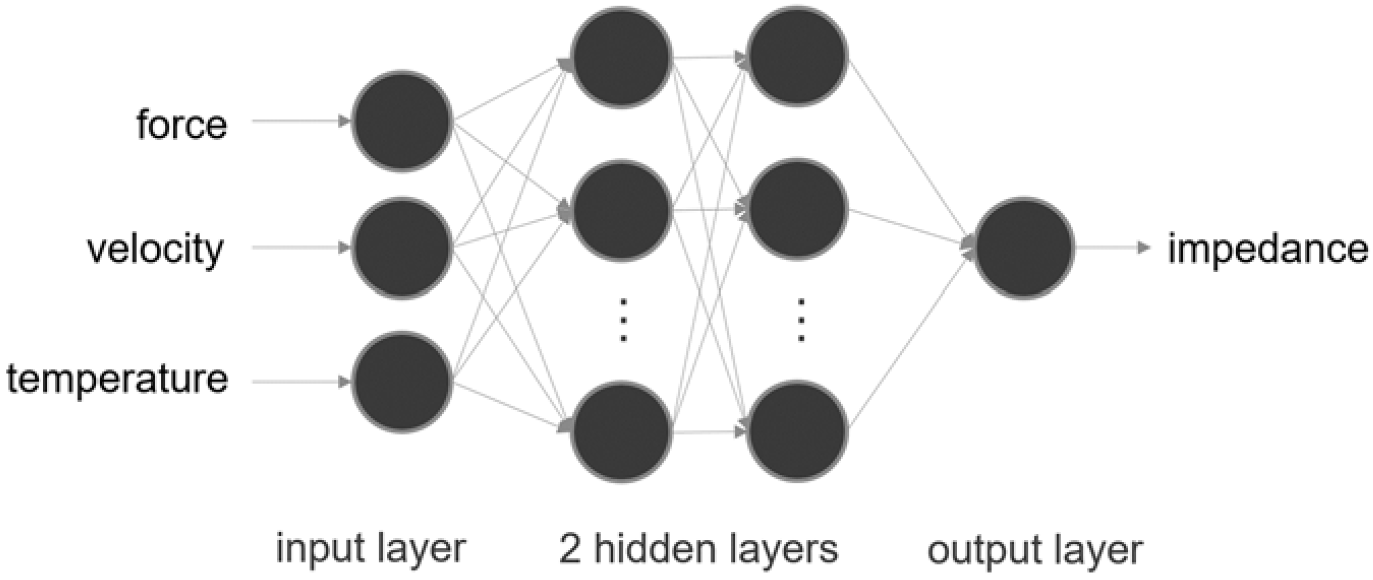
Machine learning methods are increasingly used to solve such data-driven problems due to the newly emerging possibilities. Supervised learning methods are particularly suitable for solving data-driven problems. These are presented below regarding their application in engineering sciences. The investigated methods are linear methods, tree-based methods, and neural networks, where each method maps the input matrix X on the target variable Y. Where in this context the input is temperature, velocity and force. The output is the bearing impedance.

1.2.1. Linear Regression Methods

The linear regression linearly maps correlations between input parameters and output parameters. Mathematically, the relationship for $\mathit{p}$ input parameters is formulated as follows [9]:

$$\mathit{Y}={\beta }_0+{\beta }_1{\mathit{X}}_1+{\beta }_2{\mathit{X}}_2+\dots +{\beta }_{\mathit{p}}{\mathit{X}}_{\mathit{p}}.$$

(5)

The parameters ${\beta }_{\mathit{i}}$ for $\mathit{i}=1\dots \mathit{p}$ describe the linear dependence between the different input parameters ${\mathit{X}}_{\mathit{i}}$ and the output parameter $\mathit{Y}$. These must be optimized based on the available data set. Due to the linear character of Equation (5) an optimum is guaranteed [10].

For regression problems with many input parameters, advanced linear methods like lasso regression can be used. These ensure that only input parameters that are vastly correlated with the output are included in the regression. This is done with a regularization parameter 𝜆. The optimization problem is according to [11]:

$$\mathit{F}\mathit{i}\mathit{n}\mathit{d} {\mathit{\beta }}_{\mathit{i}} \mathit{s}\mathit{u}\mathit{c}\mathit{h} \mathit{t}\mathit{h}\mathit{a}\mathit{t} {(\mathit{Y}-{\mathit{\beta }}_0-{{\displaystyle \sum }}_{\mathit{j}=1}^{\mathit{p}}{\mathit{\beta }}_{\mathit{j}}{\mathit{X}}_{\mathit{j}})}^2+ \lambda {{\displaystyle \sum }}_{\mathit{j}=1}^{\mathit{p}}\left|{\mathit{\beta }}_{\mathit{j}}\right|\Rightarrow \mathit{M}\mathit{i}\mathit{n}.$$

(6)

The first summand represents the root-squared-mean-error [9] and the second one the regularized regression parameters.

Since physical phenomena are often nonlinear, correlations with polynomial regression can also be regressed in higher dimensions [9]. This is a special form of linear regression. In the one-dimensional case, a d-order polynomial is adapted to existing data with the following equation:

$$\mathit{Y}={\mathit{\beta }}_0+{\mathit{\beta }}_1\mathit{X}+{\mathit{\beta }}_2{\mathit{X}}^2+\dots +{\mathit{\beta }}_{\mathit{d}}{\mathit{X}}^{\mathit{d}}.$$

(7)

The optimization of the parameters is still a convex optimization problem and is performed like the linear regression with iterative methods for example the gradient descent method [11].

1.2.2. Decision Trees

Decision trees are simple methods for the solution of classification and regression problems. They consist of root nodes and nodes that can be interpreted as decision points and leaves that can be described as decision results [12]. The data set is divided binary at points where a division has the highest information content. This can be described using the Gini coefficient $\mathit{G}$, where ${\widehat{\mathit{p}}}_{\mathit{m}\mathit{k}}$ stands for the proportion of the k-th class in the m-th region [11]:

$$\mathit{G}={{\displaystyle \sum }}_{\mathit{k}=1}^{\mathit{K}}{\widehat{\mathit{p}}}_{\mathit{m}\mathit{k}}\left(1-{\widehat{\mathit{p}}}_{\mathit{m}\mathit{k}}\right).$$

(8)

Decision trees can adapt very well to the training data, but when applied to the test data, this can lead to rather inaccurate results. This behavior is called overfitting and can be interpreted as memorization [11]. Possibilities to increase the generalization of the results are the modification of the algorithm to a random forest or the boosting of decision trees [12]. The random forest is based on many uncorrelated partial decision trees and is called an ensemble method. The same applies to boosting, which determines the result by weighted weak learners [11].

1.2.3. Neural Networks

The neural network is a nonlinear optimization problem. Due to its ability to learn complex facts it is used with increasing frequency for complex tasks. The basic algorithm was published several decades ago [13]. It consists of units arranged in layers. The units represent the calculation rule ${\mathit{s}}_{\mathit{k}}$:

$${\mathit{s}}_{\mathit{k}}={{\displaystyle \sum }}_{\mathit{j}}\left({\mathit{w}}_{\mathit{j}\mathit{k}} {\mathit{y}}_{\mathit{j}}\right)+{\mathit{\theta }}_{\mathit{k}}.$$

(9)

The input ${\mathit{y}}_{\mathit{j}}$ is optimized with the help of the weights ${\mathit{w}}_{\mathit{j}\mathit{k}}$ where ${\mathit{\theta }}_{\mathit{k}}$ is a bias parameter. The output ${\mathit{s}}_{\mathit{k}}$ is finally activated and passed on with activation functions [13]. Currently the rectified linear unit (ReLU) function is state of the art and used as the activation function [13]. If the output of a unit is positive, it is activated linearly and if it is less than or equal to zero, it is deactivated. Mathematically formulated, the nonlinear ReLU function is according to [14]:

$$\mathit{f}\left(\mathit{x}\right)=\max \left(0,\mathit{x}\right)=\{\begin{array}{c}{\mathit{x}}_{\mathit{i}}, \mathit{i}\mathit{f} {\mathit{x}}_{\mathit{i}}\ge 0\\ 0, \mathit{e}\mathit{l}\mathit{s}\mathit{e}\end{array} .$$

(10)

The weights ${\mathit{w}}_{\mathit{j}\mathit{k}}$ are minimized to train the neural network using nonlinear optimization algorithms. Classical methods are the stochastic gradient descent [10] and Newton methods like the limited-memory Broyden-Flechter-Goldfarb-Shanno (L-BFGS) algorithm [15,16].

The aim of the experiments was the comparison of measurement results with the analytical models from the literature to identify promising approaches for the further development of these models [3]. To limit the complexity of the analytical models in the first step, only bearings under purely radial load were tested. The difference between the extended analytical model and the measurement led to the choice of a data-based approach. In the following work, combined axial and radial loads as well as the size influence of different bearing types will be investigated [8].

2. Materials and Methods

This section presents how the data was obtained and which machine learning methods were used to describe the electrical impedance of rolling bearings.

2.1. Database

To analyze the dependency of the electric impedance of rolling bearings on operating conditions, bearings of type 6205 C3 manufactured by Schaeffler (Herzogenaurach, Germany) are tested on the test rig shown in Figure 5. The used experimental data and the test rig are described in [3], the hydraulic apply pistons 1 and 2 are capable of loading the testing apparatus with axial, radial and combined loads. Figure 6 shows the arrangement including two test bearings and another two support bearings and the location of the insulation layers. The radial load is applied to the two rolling bearings arranged in the center of apparatus and discharged via the two outer rolling bearings acting as supports. The driving AC-motor denoted by 3 in Figure 5 is controlled to the target velocity of the shaft. The temperature of the outer race is measured at all four rolling bearings in the test rig with the thermocouples indicated by 4 in Figure 5. Closed loop control is applied on the lubricant temperature, the shaft velocity and the load applying pistons of the test bench. The slip ring 5 is located on the shaft to generate a measuring circuit including inner and outer races of the roller bearing. The contact pin 6 serves as electrical contact of the outer ring to close a defined electrical circuit through the rolling bearing of interest, see Figure 6. The test apparatus is equipped with enforced circulation of the temperature controlled liquid lubricant so that the bearing is enclosed by the dielectric lubricant. The elastic coupling 7 insulates the testing apparatus from the electric drive unit to prevent interferences between the testing setup and the inverter fed motor.

Figure 6 shows the schematic cross section of the testing apparatus with the electrical test setup and the insulation layer between the apply unit and the test bearing outer races to enable a defined electrical measurement circuit. With the electrical circuit designed to measure the electrical impedance, a voltage is applied to the shaft via the slip ring using an alternating current source operated at a signal frequency ${\mathit{f}}_{{m}}=5 \mathrm{MHz}$ and a voltage amplitude ${\mathit{U}}_{{S}}=1 \mathrm{V}$. Below 3 MHz the used current probe does not work and in different test rigs skin effects were observed over 7 MHz signal frequency. When working with frequencies in the MHz range, it should be noted that inductances can always lead to errors in the measurement. These potential sources of uncertainties must be considered.

Triggered by the voltage, a current flows through the two test bearings, which is measured at each contact of the outer ring. The voltage is measured directly at the alternating current source since the voltage in the two parallel-connected bearings is the same according to Kirchhoff’s rules. The electrical impedance is determined from the measured transfer function from voltage to current. Result of the evaluation is the electrical impedance as a function of time of one second. To determine a single value for the impedance for a measuring intime instance, the median of the signal is used. The used current probe is a CT2 (Tektronix, Beaverton, OR, USA) and the voltage is measured with a Picoscope 4444 oscilloscope (Pico Technology, Cambridgeshire, UK).

To investigate the approach of Schirra et al. [6] where the technology is used to describe bearing forces, the focus of the investigations is on different load levels. The tests were performed using 6205 C3 type rolling bearings with reduced radial freeplay and the lubricant FVA Referenzöl 3A (

Table 1. Lubricant properties.

Parameter	FVA 3A
Density. 15 °C	$880-890 \raisebox{1ex}{$\mathrm{kg}$}\!\left/ \!\raisebox{-1ex}{${\mathrm{m}}^3$}\right.$
kin Viscosity, 40 °C	$85-95 \raisebox{1ex}{${\mathrm{mm}}^2$}\!\left/ \!\raisebox{-1ex}{$\mathrm{s}$}\right.$
kin Viscosity, 100 °C	$10-11 \raisebox{1ex}{${\mathrm{mm}}^2$}\!\left/ \!\raisebox{-1ex}{$\mathrm{s}$}\right.$
Viscosity index	$94$

) manufactured by Klüber Lubrication (Munich, Germany) which was investigated in detail electrically. Since the electrical impedance with capacitive behavior depends on the AC frequency, the measuring voltage was applied with a frequency of 5 MHz. The varied parameters are the speed, the oil temperature, and the radial bearing load. The bearing load was increased logarithmically from 700 to 7200 N to reflect the higher sensitivity of the measured variable at lower loads. The lower limit is determined by the minimum possible load of the test rig and the upper limit by the static load capacity of the bearing. The speed is selected with 500, 1000, 3000 and 6000 rotations per minute in different orders of magnitude of real operating conditions. The temperature is selected at a lower level with 35 °C and a higher level with 65 °C. To consider the influence of tolerances, the tests are carried out with eight bearings. The varied parameters can be found in

Table 2. Test parameters of the screening campaign (Taken from [3]).

Bearing Type	$\mathbf{Radial} \mathbf{Force} {\mathit{F}}_{\mathit{R}}$	$\mathbf{Rotation} \mathbf{Speed} \mathit{n}$	$\mathbf{Temperature} \mathit{T}$
8x 6205 C3	$20 \mathrm{logarithmic} \mathrm{steps} 700–7200 \mathrm{N}$	$$\begin{gathered} 500, 1000, \\ 3000, 6000{ \min }^{-1} \end{gathered}$$	$35$$\mathrm{and} 65 °\mathrm{C}$

and results are shown in Schirra et al. [3].

2.2. Regression Method

This section describes the pre-processing of the data and gives an overview of the models used, which are finally evaluated. The pre-processing is applied to filter the signal and thus reduce the influence of outliers, which is described in the following.

2.2.1. Pre-Processing

Due to natural errors in data acquisition, the data must be prepared for further analysis in the first step since models can react sensitively to measurement outliers [17]. During the measurement, the electrical impedance is measured over one second. As can be seen in Figure 7, the impedance value is not constant over one second and an evaluation procedure is used to determine a value. As Martin et al. [1] have shown, the frequencies that occur depend on the rotating components in the rolling bearing, and their influence should be neglected when investigating the absolute value. For this reason, the median of the measurement over one second is chosen to determine the absolute measured value [3].

In the next step the whole data set is rescaled by standardization. Machine learning algorithms converge faster by adjusting the data [15]. A dimensional reduction is not necessarily due to the small amount of data and the physical presumptions.

2.2.2. Model Predictors Selection

Due to the design of the experiments, the available input parameters are the radial force acting on the rolling bearing, the oil temperature of the bearing and the shaft speed [6]. All measured parameters have meaningful effects on the measured output parameter, the electric impedance [18,19]. These assumptions can be confirmed by correlation analyses. In addition, an uncorrelatedness between the different input parameters can be affirmed. Thus, all measured quantities can be used for the prediction of the impedance. Due to the physically based assumptions, this is a grey box model, which approximates the so far insufficient analytical correlation between input and output.

Based on the information about the excitation speed contained in the measured impedance, there is the assumption that the measured rotational speed can be substituted by the amplitude spectrum of the impedance [1,2,20]. Investigating this hypothesis from a machine learning perspective can serve as a basis for further research in this area. By showing that the measured velocity can be replaced with the frequency of the impedance signal using machine learning algorithms, it should be possible to predict the bearing load without velocity measurement data in the future, since the impedance is measured for load prediction anyway [1].

The amplitude spectrum is calculated by a fast Fourier transform of the one second long, high-frequency sampled time signal. Figure 8 shows the typical frequency spectrum of rolling bearings. Here the amplitude is plotted over the order, where the measured frequencies are related to the rotational speed $\mathit{n}$.

Thus, two possible cases of impedance regression are created. Case 1 uses the radial force, the temperature and the rotational speed as input parameters and Case 2 the radial force, the amplitude spectrum of the impedance and the temperature.

2.2.3. Models

The two cases described above are examined for their accuracy using the methods linear regression, polynomial regression grade 2, random forest, gradient boost, and feedforward neural network. The operating principles of these methods are already presented in Section 1.2. Although there are more sophisticated machine learning methods available in literature, the methods used here are considered appropriate for the given purpose of bearing impedance regression. For this reason, interaction terms and higher-order terms are not considered.

The models are implemented in python. Thereby, all machine learning algorithms used are imported from the Scikit-learn library. In addition, the libraries pandas and numpy are used for data processing and matplotlib for visualization. The parameters of the models are determined through a grid search algorithm. As a result, the random forest is set to a tree count of 250. The maximal depth per tree is unlimited. The gradient boost algorithm is set to 200 estimators with a maximum depth of 2. The feedforward neural network is visualized in Figure 9. Resulting from the grid search, it has 2 hidden layers with 100 neurons per layer. The activation functions are defined as rectified linear units. To prevent overfitting of the neural network, training is performed using L2 regularization with a penalty parameter of 0.0001.

The results of all trained models are characterized and compared with each other using the evaluation parameter root mean squared error (RMSE) as a goodness of regression method. The RMSE is defined as follows [9]:

$$\mathrm{RMSE}=\sqrt{\frac{1}{\mathit{n}}{{\displaystyle \sum }}_{\mathit{i}=1}^{\mathit{n}}{\left({\widehat{\mathit{y}}}_{\mathit{i}}-{\mathit{y}}_{\mathit{i}}\right)}^2}.$$

(11)

2.2.4. Learning Process

The learning process corresponds to the train-test split, so that the algorithm learns based on 50 percent of the data (640 measuring points) and tests what has been learned based on 50 percent of the data (640 measuring points). All tuning parameters are determined by a grid search, structured for minimum error, if required. The grid search thereby is applied to a 5-fold cross-validated split of the training data. Reason for this approach is to achieve an optimal bias-variance tradeoff. Finally, the pre-set models are evaluated based on 25 test runs, so that information can be given about the expected value of the accuracy of the different models and their standard deviation. This procedure ensures that the variance-bias trade-off is as ideal as possible [21]. The variance-bias trade-off refers to the relationship between the accuracy and generalization of the model. It can be shown that an ideal point can be found, but the error can never become zero. The reason for this is the statistical measurement noise of the measured values [11].

3. Results and Discussion

Based on the different model approaches, the regression results are compared. Different aspects such as accuracy and generalizability of the algorithms are discussed. For each case one single bearing and all eight measured bearings are considered in one model and the errors are compared.

Table 3. Accuracy of algorithms with measured velocity.

Input	FVT for 1 Bearing in %	FVT for 8 Bearings in %
Linear regression	96.92	95.49
Polynomial regression	98.62	97.15
Random forest	97.47	98.68
Gradient boost	98.40	97.97
Neural network	97.92	98.77

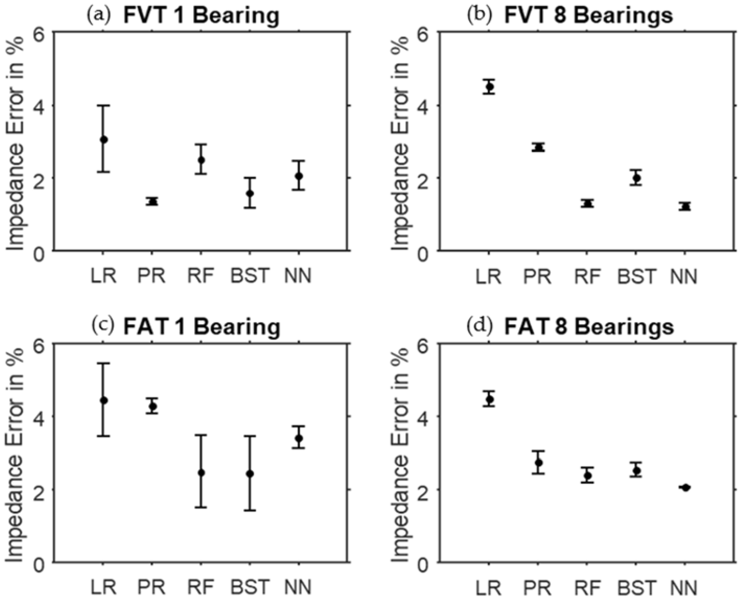
shows the accuracy of the impedance prediction depending on the parameters and the regression method used. In Figure 10 the value of the prediction error is reported. F stands for radial force, V for velocity, T for temperature and A for impedance spectrum of the impedance Z. The abbreviations of the input parameters are FVT 1 or FVT 8. The input parameters are load (F) velocity (V) temperature (T). The designation FVT 1 considers data measured with only one bearing (160 measuring points). FVT 8 considers the whole data measured with the eight bearings examined in the test (1280 measuring points). The comparison of the accuracies will show whether bearing tolerances caused by manufacturing or the assembly process have a major influence on the measurement result.

Linear regression performs least well in the FVT investigation. All other algorithms used deliver very high accuracies in the range between 97 % and 99 % for both one and eight bearings. A significant trend cannot be identified when comparing one and eight bearings in use.

Table 4. Accuracy of algorithms with frequency spectrum.

Input	FAT for 1 Bearing in %	FAT for 8 Bearings in %
Linear regression	95.55	95.51
Polynomial regression	95.70	97.24
Random forest	97.50	97.60
Gradient boost	97.55	97.45
Neural network	96.58	97.92

shows the accuracy of the impedance prediction depending on the parameters and the regression method used. With the abbreviations FAT 1 and FAT 8 the input parameter velocity is replaced by the amplitude spectrum (A) of the bearing impedance. The reason is the possible use case for the technology, Schirra et al. [3] mentioned. Thereby, bearing impedance is measured to predict bearing loads for predictive maintenance applications. The question is if an additional sensor for the velocity is needed or the amplitude spectrum of the impedance contains this information.

From the accuracy results shown in Table 3 and Table 4 it can be concluded that a second-order polynomial yield more accurate results than linear regression. Thus, it can be concluded that the physical relations for at least one input parameter are nonlinear, otherwise the match would be perfect to the interpolation chosen. For complex models with many input parameters, as in the case of the amplitude peak, the lasso extension must be used for the linear regression, because not every amplitude correlates significantly with the impedance and therefore gives bad results for a non-weighted approach. The random forest and gradient boost algorithms can be used for both FVT and FAT as they are decision tree- based ensemble methods that automatically identify relevant parameters [11].

The various machine learning algorithms offer varying degrees of transparency. Linear and polynomial regression offer good comprehensibility due to their simple structure. Random forest and gradient boost are tree-based methods, which are difficult to interpret due to the large number of trees used for prediction. NNs are the least interpretable in comparison to the other models due to their complex architecture. Furthermore, these properties are related to the algorithms’ generalizability. When using test data that is not within the range of the training data, the algorithms behave in different ways. Linear and polynomial regression extrapolate relatively well based on their simple defined structure. The prediction of the neural network outside of the training range is rather erratic. However, these extrapolation characteristics are not discussed in detail here, since these are known properties of the machine learning algorithms. The test data used for the results shown here originates from the same data set as the training data. Therefore, extrapolation effects do not arise in this case.

It turns out that algorithms based on a single bearing have about the same quality as for a stack of bearings, so that the training can be done individually for a bearing or a pre-trained algorithm can be considered over many bearings. In addition, bearing tolerances and the assembly process do not have a major influence on the measurement result. An overview of the expected error in all investigated models can be found in Figure 10. In addition to the mean error of the predicted impedance, its standard deviation is shown.

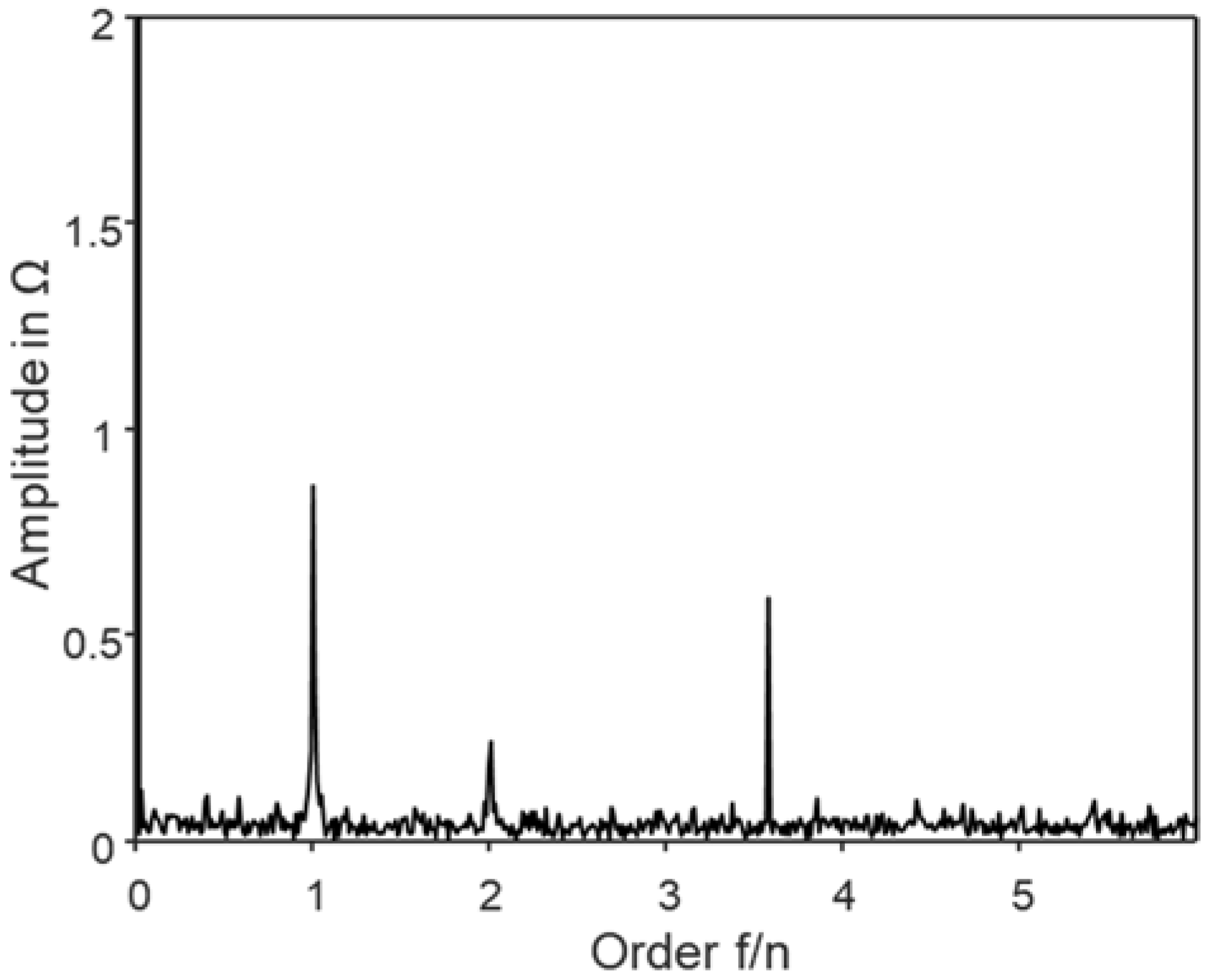
Based on the test data it seems, that random forest, gradient boosting and neural network are superior to both linear and polynomial regression in terms of their prediction results. But looking at the higher variance of the sensors in comparison to the machine learning methods the output even of the best algorithm can vary. Based on the results obtained the following observations are made: Depending on the test case, different algorithms perform particularly well. The standard deviation with only a very limited number of bearing is in generally higher compared to the use of eight or more bearings. This can be caused by the different amount of data available for training. The machine learning algorithms are able to obtain information about the excitation frequency on the amplitude spectrum (Figure 10c,d), so that a speed measurement of the shaft for impedance determination can be omitted at the cost of about 1% accuracy. Ensemble methods are the most accurate for the problems at hand. However, it should be mentioned that ensemble methods do not learn on-line but can only be used for closed data sets. The neural network always delivers predictions with above-average accuracy and is therefore the most suitable algorithm for the determination of the electrical impedance.

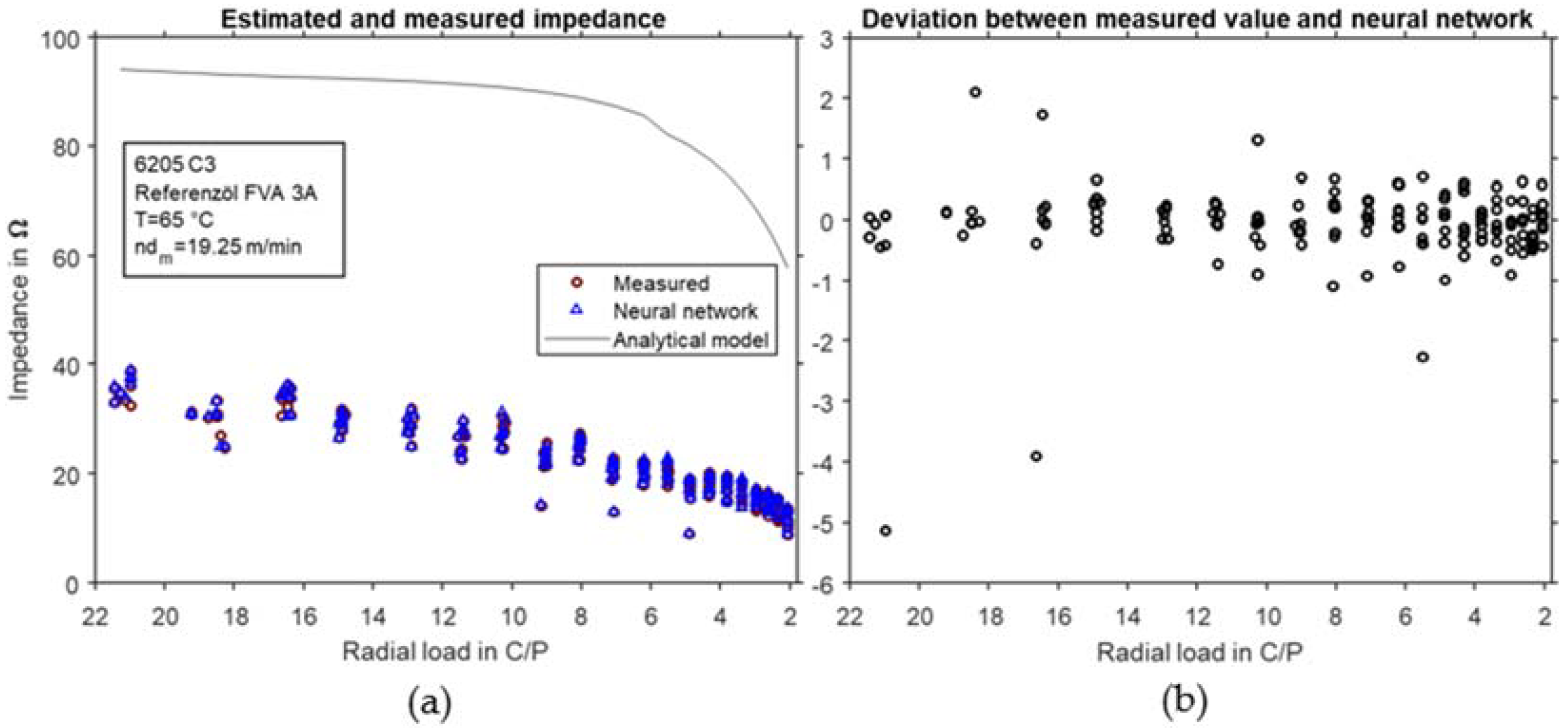
An example of predictions made by a neural network compared to actual measured impedances is shown in Figure 11. The accuracy is 98.97%. Furthermore, the well calculable correlation between the electrical impedance and the operating conditions shows that the impedance can also be an additional influencing variable for determining the remaining useful life of rolling bearings, as shown in [22]. The analytical model of Schirra et al. [3] exhibits an almost constant offset to the measurement results, which is nearly independent of temperature and rotational speed. It is clearly shown in in Figure 11 that the description with a neural network does not have the observed offset between the measurement and the analytical calculation. In addition, the description with the neural network has the advantage that every single measuring point can be described with its exact temperature. In the experiment, the temperature is set to 65 °C, but the control is only accurate to 1 °C, so deviations by this difference are possible. The analytical model has the temperature of 65 °C as input parameter, while the neural network has the exact, measured temperature as input parameter for each individual point. Thus, the uncertainty that is introduced into the analytical calculation by the control is notably reduced here.

In general the accuracy of the load predictions by either machine learning method is the range of measuring accuracy of the test device. Hence, it can be concluded, that from a practical perspective all methods applied in this paper lead to the same quality of bearing load estimates, which is on the order of the total measurement error of the apparatus. The prediction accuracy for the rotational speed is independent from the accuracy of bearing load prediction since only the governing orders in the measured spectrum are analysed, the absolute value or the phase angle of the impedance is here only of minor importance. As an overall estimate the rotational speed can be calculated with a precision of 95% over the complete operational range of the bearing.

4. Conclusions

Even though the accuracy of analytical calculations of bearing impedance has already been improved in previous publications, there is still a notable deviation from the real measurement data in the analytical calculations, leading to an off-set which is almost constant for the operational range analyzed so far. For this reason, the approach chosen here is to predict the bearing impedance using machine learning algorithms. As shown, these data-based approaches achieve much higher accuracies than the current analytical models and reduce the error to 2% as a rule of thumb. Within the compared machine learning algorithms, the neural network performs particularly well.

In addition to the prediction of the bearing impedance, it is also shown that the rotational speed can be predicted with high accuracy from the frequency spectrum of the bearing impedance. Thus, it is shown that in future investigations the direct measurement of the rotational speed is not mandatory, since it can be calculated from the measured bearing impedance.

Consequently, in the present paper the example of the bearing impedance demonstrates, that the deficits of analytical methods can be compensated with the help of data-driven algorithms. Since the underlying physics are taken into account when selecting the relevant parameters, the models used here can be categorized as so-called grey-box models.

References

1. Martin, G.; Schirra, T.; Kirchner, E. Experimental High Frequency Analysis of the Electric Impedance of Rolling Bearings. In Proceedings of the Bearing World, Frankfurt, Germany, 19–23 October 2020. [Google Scholar]
2. Gemeinder, Y.; Schuster, M.; Radnai, B.; Sauer, B.; Binder, A. Calculation and validation of a bearing impedance model for ball bearings and the influence on EDM-currents. In Proceedings of the IEEE 2014 International Conference on Electrical Machines (ICEM), Berlin, Germany, 2–5 September 2014; pp. 1804–1810. [Google Scholar] [CrossRef]
3. Schirra, T.; Martin, G.; Puchtler, S.; Kirchner, E. Electric impedance of rolling bearings—Consideration of unloaded rolling elements. Tribol. Int. 2021, 158, 106927. [Google Scholar] [CrossRef]
4. Furtmann, A.; Poll, G. Evaluation of Oil-Film Thickness Along the Path of Contact in a Gear Mesh by Capacitance Measurement. Tribol. Online 2016, 11, 189–194. [Google Scholar] [CrossRef] [Green Version]
5. Jablonka, K.; Glovnea, R.; Bongaerts, J. Quantitative measurements of film thickness in a radially loaded deep-groove ball bearing. Tribol. Int. 2018, 119, 239–249. [Google Scholar] [CrossRef]
6. Schirra, T.; Martin, G.; Vogel, S.; Kirchner, E. Ball Bearings as Sensors for Systematical Combination of Load and Failure Monitoring. In International Design Conference—Design 2018; Universität Zagreb, The Design Society: Glasgow, UK, 2018; pp. 3011–3022. [Google Scholar] [CrossRef]
7. Hamrock, B.J.; Dowson, D. Ball Bearing Lubrication—The Elastohydrodynamics of Elliptical Contacts; Wiley: New York, NY, USA, 1981. [Google Scholar]
8. Schirra, T. Phänomenologische Betrachtung der Sensorisch Nutzbaren Effekte am Wälzlager—Einfluss Unbelasteter Wälzkörper auf die Elektrische Impedanz. Ph.D. Thesis, Technische Universität Darmstadt, Darmstadt, Germany, 2021. [Google Scholar]
9. Géron, A. Hands-on Machine Learning with Scikit-Learn and TensorFlow. Concepts, Tools, and Techniques to Build Intelligent Systems, 1st ed.; O’Reilly: Beijing, China; Boston, MA, USA; Farnham, UK; Sebastopol, CA, USA; Tokyo, Japan, 2017. [Google Scholar]
10. Ruder, S. An Overview of Multi-Task Learning in Deep Neural Networks. arXiv 2017, arXiv:1706.05098. [Google Scholar]
11. James, G.; Witten, D.; Trevor, H.; Tibshirani, R. An Introduction to Statistical Learning. With Applications in R; Springer Texts in Statistics, 103; Springer: New York, NY, USA, 2013. [Google Scholar]
12. Quinlan, J. Decision Trees as Probabilistic Classifiers. In Proceedings of the Fourth International Workshop on MACHINE LEARNING; Elsevier: Amsterdam, The Netherlands, 1987; pp. 31–37. [Google Scholar]
13. Kröse, G.; Smagt, P. An Introduction to Neural Networks; University of Amsterdam: Amsterdam, The Netherlands, 1996. [Google Scholar]
14. Nwankpa, C.; Ijomah, W.; Gachagan, A.; Marshall, S. Activation Functions: Comparison of trends in Practice and Research for Deep Learning. arXiv 2018, arXiv:1811.03378. [Google Scholar]
15. Liu, D.; Nocedal, J. On the limited memory BFGS method for large scale optimization. In Mathematical Programming 45; SpringerLink: Berlin/Heidelberg, Germany, 1985; pp. 503–528. [Google Scholar] [CrossRef] [Green Version]
16. McCaffrey, J. How to Standardize Data for Neural Networks. Visual Studio Magazine. 2014. Available online: https://visualstudiomagazine.com/articles/2014/01/01/how-to-standardize-data-for-neural-networks.aspx (accessed on 17 December 2021).
17. Baumann, S.; Klingauf, U. Modeling of aircraft fuel consumption using machine learning algorithms. CEAS Aeronaut. J. 2020, 11, 277–287. [Google Scholar] [CrossRef]
18. Radnai, B.; Gemeinder, Y.; Kiekbusch, T.; Sauer, B.; Binder, A. Schädlicher Stromdurchgang—Abschlussbericht zum FVA-Vorhaben 650/I; Forschungsvereinigung Antriebstechnik e.V. (FVA): Frankfurt, Germany, 2015. [Google Scholar]
19. Schirra, T.; Martin, G.; Kirchner, E. Untersuchung Elektrischer Eigenschaften von Wälzlagern zur Entwicklung eines Sensorlagers; VDI-Fachtagung Wälz- und Gleitlager: Schweinfurt, Germany, 2019. [Google Scholar]
20. Neu, M.; Harder, A.; Kirchner, E. Sensorische Eigenschaften von Wälz- und Gleitlagerungen—Beherrschen von Unsicherheiten von und Durch die Zusatzfunktion; VDI-Fachtagung Wälz- und Gleitlager: Schweinfurt, Germany, 2019. [Google Scholar]
21. Pedregosa, F.; Varoquaux, G.; Gramfort, A.; Michel, V.; Thirion, B.; Grisel, O.; Blondel, M.; Prettenhofer, P.; Weiss, R.; Dubourg, V.; et al. Scikit-Learn: Machine Learning in Python. J. Mach. Learn. Res. 2011, 12, 2825–2830. [Google Scholar]
22. Mehringskötter, S.; Preusche, C. Consideration of Variable Operating States in a Data-Based Prognostic Algorithm. In Proceedings of the 2019 IEEE Aerospace Conference, Big Sky, MT, USA, 2–9 March 2019. [Google Scholar] [CrossRef]
Figure 1. Concept of a sensor bearing by Martin et al. (Adapted with permission from ref. [1]).
Machines 10 00156 g001
Figure 2. Electrically equivalent circuit diagrams of a rolling contact depending on the lubrication condition. (Adapted with permission from ref. [6]).
Machines 10 00156 g002
Figure 3. Modelling of a rolling bearing as capacitor network for hydrodynamic friction. (Adapted with permission from ref. [6]).
Machines 10 00156 g003
Figure 4. Load distribution for a radially loaded ball bearing (Reprinted with permission from [8]).
Machines 10 00156 g004
Figure 5. Bearing test cell with loading apparatus, measurement installation and drive unit (Adapted with permission from ref. [3]).
Machines 10 00156 g005
Figure 6. Schematic cross section of the mechanical setup and its insulation concept (Reprinted with permission from ref. [3]).
Machines 10 00156 g006
Figure 7. Exemplary measurement of the impedance over one second (Reprinted with permission from ref. [1].)
Machines 10 00156 g007
Figure 8. Exemplary representation of the frequency spectrum of the electrical impedance of rolling bearings (Reprinted with permission from ref. [1].)
Machines 10 00156 g008
Figure 9. Neural network with the chosen parameters for FVT (force, velocity, temperature) regression.
Machines 10 00156 g009
Figure 10. Mean value and standard deviation of the examined methods (linear regression LR, polynomial regression PR, random forest RF, gradient boost BST, neural network NN) for the input parameters FVT 1 (a), FVT 8 (b), FAT 1 (c), FAT 8 (d).
Machines 10 00156 g010
Figure 11. Measured impedance and predictions from the neural network in comparison to the analytic model on the left (a) and the deviation between analytical model and neuronal network on the right (b).
Machines 10 00156 g011