Abstract
Additive manufacturing technologies present a series of advantages such as high flexibility, direct CAD to final product fabrication, and compact production techniques which make them an attractive option for fields ranging from medicine and aeronautics to rapid prototyping and Industry 4.0 concepts. However, additive manufacturing also presents a series of disadvantages, the most notable being low dimensional accuracy, low surface quality, and orthotropic mechanical behaviour. These characteristics are influenced by material properties and the process parameters used during manufacturing. Therefore, a predictive model for the characteristics of additive manufactured components is conceivable. This paper proposes a study on the feasibility of implementing Deep Neural Networks for predicting the dimensional accuracy and the mechanical characteristics of components obtained through the Fused Deposition Modelling method using empirical data acquired by high precision metrology. The study is performed on parts manufactured using PETG and PLA materials with known process parameters. Different Deep Neural Network architectures are trained using datasets acquired by high precision metrology, and their performance is tested by comparing the mean absolute error of predictions on training and validation data. Results show good model generalisation and convergence at high accuracy, indicating that a predictive model is feasible.
1. Introduction
Additive manufacturing technologies are becoming an essential tool in a wide variety of fields ranging from medicine and aeronautics to industry 4.0 concepts, rapid prototyping, reverse engineering, and hobby use. This rapid increase in the exploitation of additive manufacturing techniques is a direct result of the many advantages presented by these technologies, which include high flexibility, low cost, direct computer-aided design (CAD) to finished product manufacturing, reduced tooling requirements, the capability of realising high complexity geometries in a short time and at low cost, etc. At the same time, additive manufacturing techniques also suffer from a series of disadvantages, most notably low dimensional accuracy, low surface quality, and orthotropic material behaviour. The Fused Deposition Modelling (FDM) in particular has seen a great increase in utilisation, mostly due to the ease of use and availability of low-cost machines and raw material for this technique. Due to the low cost of the machines and materials, the FDM technique is becoming important for rapid prototyping, hobby use, manufacturing of replacement parts, and even as a supplement for the more productive technologies such as Injection Molding, being employed in the form of “3D printing farms” composed of many FDM machines to compensate for the low productivity, thus enhancing the flexibility of the production lines where they are implemented. However, of all the additive manufacturing techniques, FDM suffers the most from the disadvantages mentioned above; therefore, extensive postprocessing of the manufactured parts is employed, which is costly and time consuming.
2. State of the Art
Research has been done [1] with good results on increasing the accuracy of FDM manufactured parts by fabricating components followed by parametric compensation of the 3D model using data obtained by high precision metrology.
Studies by Yadav D. et al. [2] have been performed on improving the tensile strength of additive manufactured parts by employing neural networks trained on parameters such as infill density, extrusion temperature, and material density. The study was performed on parts obtained from materials such as Acrylonitrile Butadiene Styrene (ABS) and Polyethylene Terephthalate Glycol (PETG) and showed good results, improving the tensile strength by 4.54% in subsequent samples.
Research on predicting optimal manufacturing parameters by Deshwal S. et al. [3] to increase the tensile strength of parts obtained from Polylactic Acid (PLA) material has been performed by training neural networks on process parameters such as nozzle temperature, printing Speed, and infill density. The study reported an increase in tensile strength of ~2 MPa using predictions from a neural network trained at 99.89% accuracy.
Research studies by O.A.Mohamed et al. [4] have been performed regarding the ability of artificial neural networks to predict dimensional characteristics of parts obtained through the FDM process by analysing parameters such as slice thickness, the number of perimeters, deposition angle, part print direction, and raster to raster air-gap. The study compared the precision of neural networks to classic regression techniques and showed that neural networks can account for dimensional deviations.
Tura A.D. et al. [5] performed studies on predicting the effects on surface roughness of FDM process parameters such as layer thickness, orientation angle, and infill angle with good results showing a high impact of layer thickness on surface roughness and the ability of neural networks to predict the effects.
Lyu et al. [6] researched the ability of neural networks to predict dimensional characteristics of FDM manufactured parts by analysing the complex relationship between nozzle temperature, layer thickness, and infill density and their effects on dimensional characteristics.
Previous research by A. D. Sterca et al. [7] was conducted to determine if the main FDM process parameters, e.g., temperature, speed, and part/layer orientation, influence the dimensional accuracy of 3D printed parts. The study was performed using regression analysis on data obtained by high precision metrology on a set of test parts. The study showed a strong correlation between the main process parameters and dimensional accuracy. The study also showed that 40% of the dimensional deviation from nominal is caused by a combination of factors that are not accounted for and by complex interactions between parameters which can not be modelled by a simple linear regression function.
Based on previous research [7], a correlation exists between geometric feature size and dimensional deviation, accounted for by the material shrinkage rate.
The research performed in this study characterises the materials used in terms of their shrinkage rate with the aim of increasing the accuracy of dimensional deviation predictions. In addition, the study takes printing speed into account, which has been shown to affect dimensional deviations through a combination of effects [7]. Part warping has been shown to be the most important factor in dimensional accuracy and is strongly influenced by part and layer cooling times and material shrinkage rates. Cooling times for both parts and layers are determined by a number of parameters such as printing speed, layer cooling fan speed, nozzle temperature, and heated bed temperature. These parameters all affect the temperature gradient throughout the part and thus the degree to which the part warps. Therefore, this study proposes including all of these parameters as inputs for training the neural network, filling gaps in the field by accounting for the fundamental parameters such as printing speed and material shrinkage rate, which have been shown to influence part quality but have not been studied in a correlative manner. The study also proposes the development of separate neural networks for each predicted characteristic (mechanical behaviour, dimensional deviations) in a cross-platform environment, allowing for modularity and the ability to develop more complex networks that can make design decisions using predictions produced by the different modules.
The study presented in this paper aims to determine the ability of artificial neural networks to learn and approximate the complex functions needed to predict dimensional deviations and mechanical behaviour of parts obtained by the FDM process using the main process parameters as well as material properties as inputs and empirical data obtained from high precision metrology and tensile strength measurements as outputs. A predictive mathematical model can provide information in the form of deviation from nominal, which can be used to improve dimensional accuracy in the design stage by applying corrections based on predictions to a parametric 3D model of the part, reducing or eliminating the need to manufacture and measure a series of parts to compensate for dimensional accuracy. Predictions of the mechanical characteristics of 3D printed parts can be used in the design process for guiding decisions regarding layer orientation and feature dimensions to ensure proper mechanical behaviour of the manufactured part. The predictions for dimensional and mechanical characteristics can be used to train an additional artificial neural network to provide a good compromise between dimensional accuracy and mechanical properties.
The ability to predict the characteristics of additive manufactured parts can increase the quality and interchangeability of these components and can even lead to a tolerance standard for components obtained through these techniques.
3. Materials and Methods
A test part geometry is designed and manufactured from PETG and PLA materials using different printing speeds, nozzle temperatures, and orientations. The parts obtained by the FDM process are measured using Coordinate measuring techniques and 3D scanning techniques. Tensile strength measurements are performed on the parts to determine if and how the mechanical characteristics are affected by different process parameters.
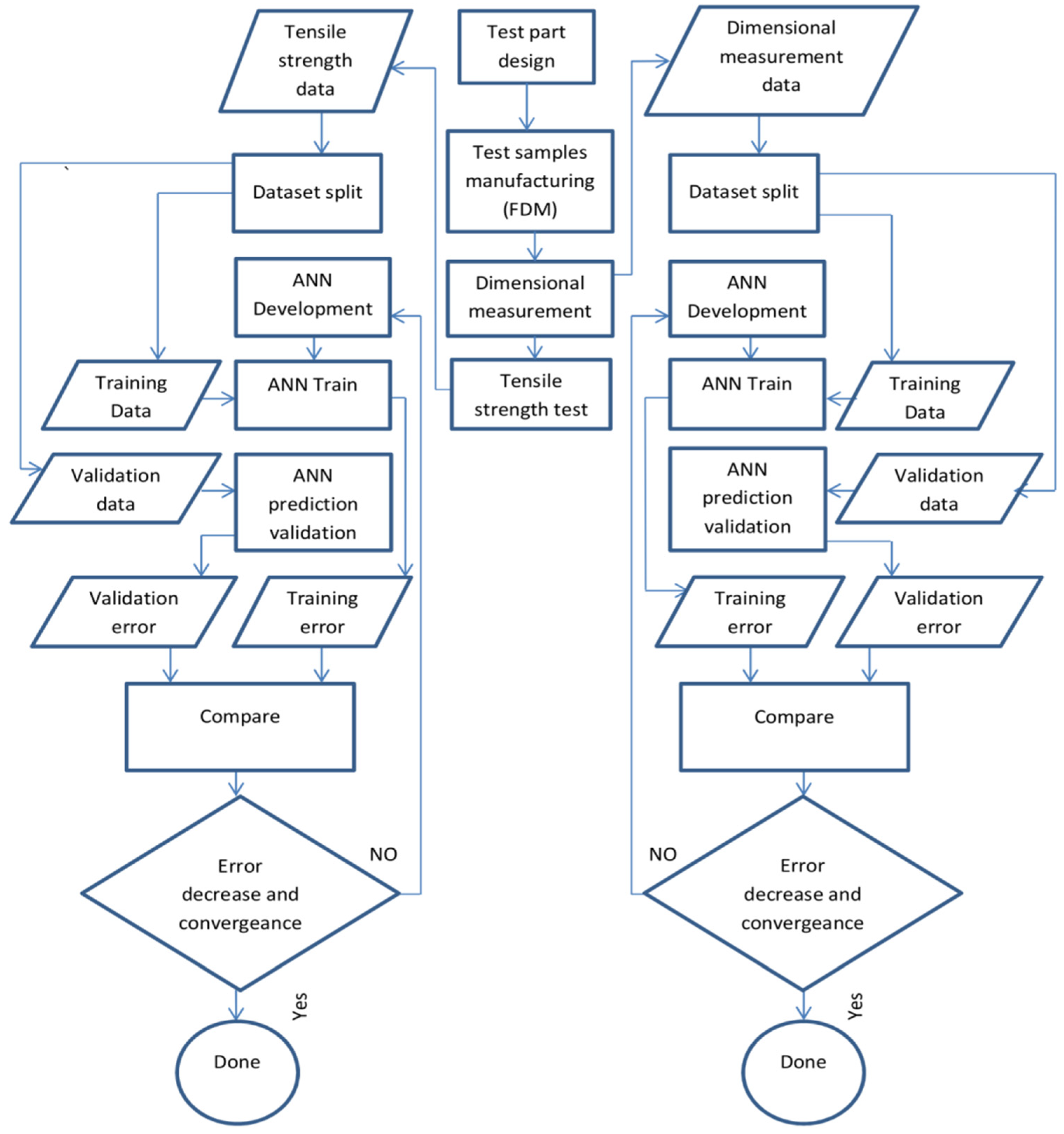
Different Artificial Neural Network (ANN) architectures are developed and trained using empirical data acquired through measurements and material properties data obtained from the manufacturer and public databases. The performance of Artificial neural networks is determined by comparing predictions with real-world data. The predictions can be tested either by manufacturing a new set of parts to be used as test data or by splitting the existing dataset into Training and Validation Data. In this study, the second method will be used, splitting the dataset into two subsets, 80% being used as training data and 20% for validation. The data splitting is done at random, providing an unbiased test of the performance. The performance of the ANN is determined by the ability of the model to generalise [8]. The experimental process is described in the flowchart presented in Figure 1, where the entire experimental process from part design through measurement, data management, and neural network training and performance analysis processes are set in order. Neural network performance analysis through comparisons between training accuracy and validation accuracy can be done at the same time after each training iteration, or a network can be validated on new data after the training has been performed to a satisfactory accuracy. This study performs validation after each training iteration, providing a plot of the performance at every step. This allows for close monitoring of the performance and early identification of unsatisfactory models.
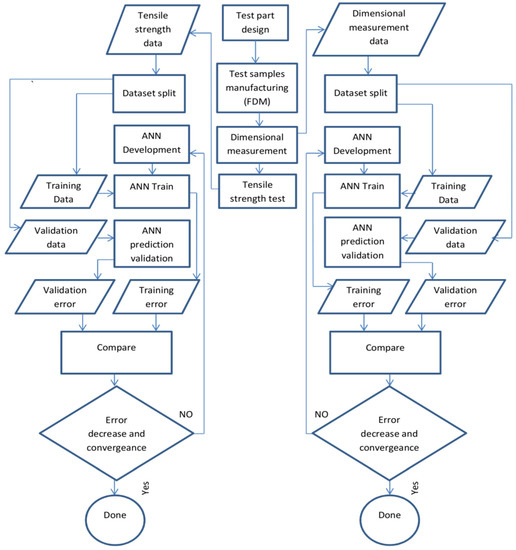
Figure 1.
Experimental process flowchart.
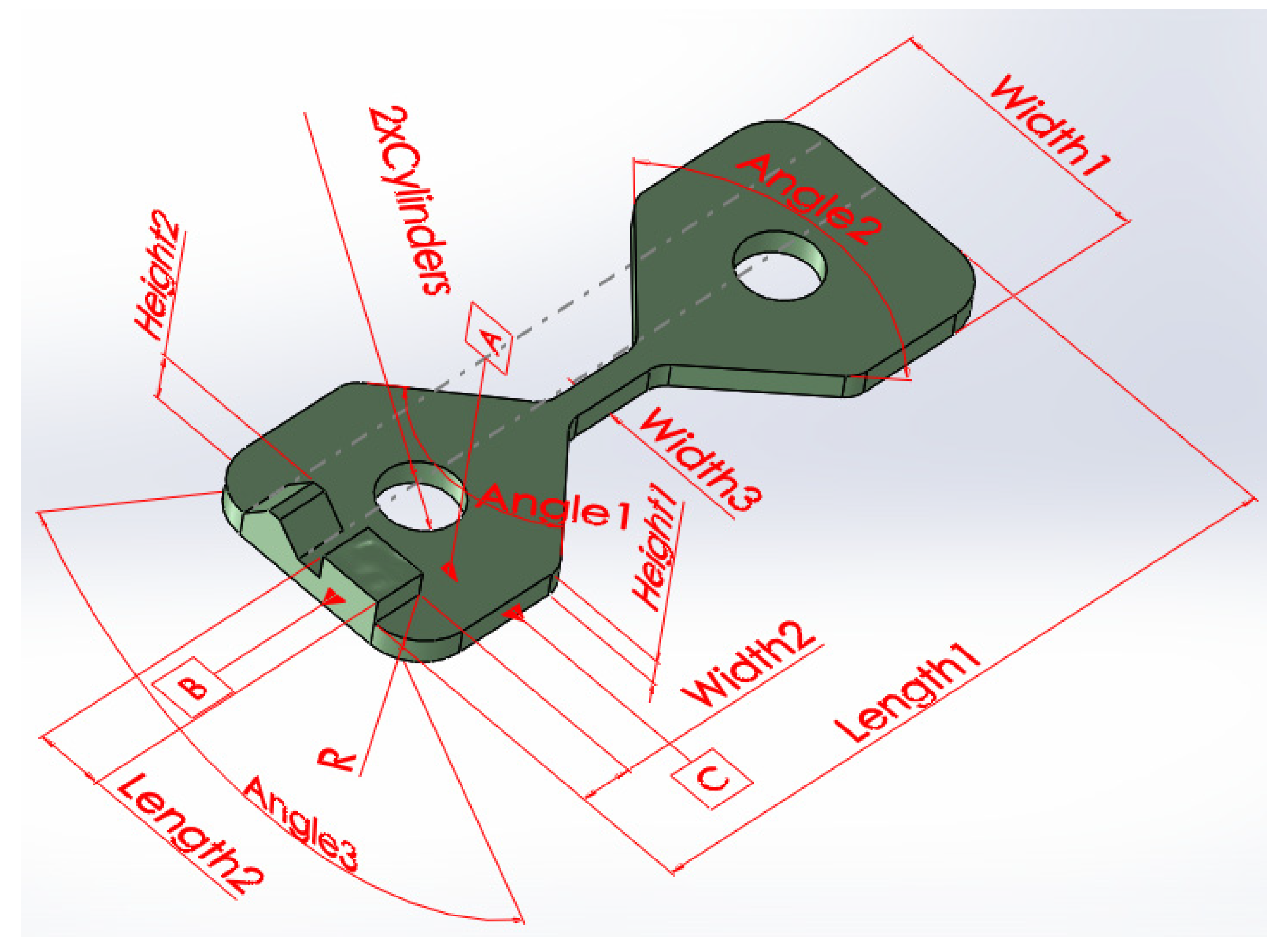
A test part presented in Figure 2 is designed using the SolidWorks [9] software suite. The geometry of the test part is chosen to amplify the effects of process parameters on the dimensional and mechanical characteristics of the manufactured parts. A high length to thickness ratio increases the effect of part warping during cooling. A low surface area zone (marked as Width3 in Figure 2) is used as a breaking point for tensile strength measurements as well as for amplifying the effects of different parameters on surface quality. A transition from a low to a high surface area defined by Angle1 and Angle2 is used to determine the variation of surface quality while at the same time providing a possible clamping feature for tensile strength measurements. The test part geometry includes different linear and circular features, which can provide measurement data for different layer orientations. The part is designed and annotated according to ISO 1101 [10].
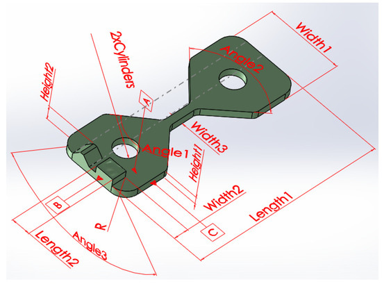
Figure 2.
Test part CAD model.
A total of 36 parts are manufactured, 12 using DevilDesign PETG material [11] and 24 using DevilDesign PLA [12]. The parts are manufactured on two FDM 3D printers, an Anycubic ProMax2 [13] presented in Figure 3a for the PLA parts and a LeapfrogXS [14] as seen in Figure 3b for the PET-G parts. Manufacturing is carried out in sets of two parts simultaneously, one in horizontal and one in a vertical orientation, as seen in Figure 3b, to ensure identical conditions for both orientations. The parameters of nozzle temperature and print speed is varied for each set of parts according to Table 1. and the values are chosen to represent the minimum, medium, and maximum temperature and speed for the material and machine used. A fractional factorial design is preferred to force the neural network to learn correlative functions. The parameter variation for the fractional factorial design is chosen in a range to be statistically significant, providing two extremes (minimum and maximum) and a median point. A minimum of three sample points for the values is needed for the neural network to identify them as variable instead of categorical data. If a neural network shows good performance in terms of generalisation and convergence, a full factorial design can be implemented to increase the prediction accuracy. All parts were manufactured using a 0.5 mm nozzle, 0.25 mm layer height, 5 mm wall thickness, 1 mm top/bottom thickness, and 30% infill using a linear infill pattern. The 5 mm wall thickness ensures a 100% infill for the 5 × 5 mm area designated as the breaking point for tensile strength tests. A sample of the manufactured parts can be seen in Figure 3c.
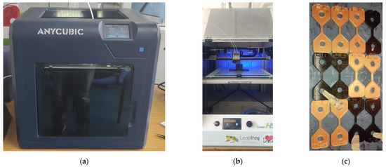
Figure 3.
Machines used for manufacturing test parts, (a) Anycubic 4Max Pro 2.0, (b) Leapfrog Creatr HS and (c) sample of manufactured parts.

Table 1.
Process parameters used for manufacturing test part pairs.
The naming of the test parts within the context of this paper is done according to Table 1 and takes the form of Temp_Speed_Orientaion_Material; thus, a part with the designation 210_90_V_PLA is identified as the test part manufactured with a nozzle temperature of 210 °C at a printing speed of 90 mm/s in the vertical orientation using PLA material.
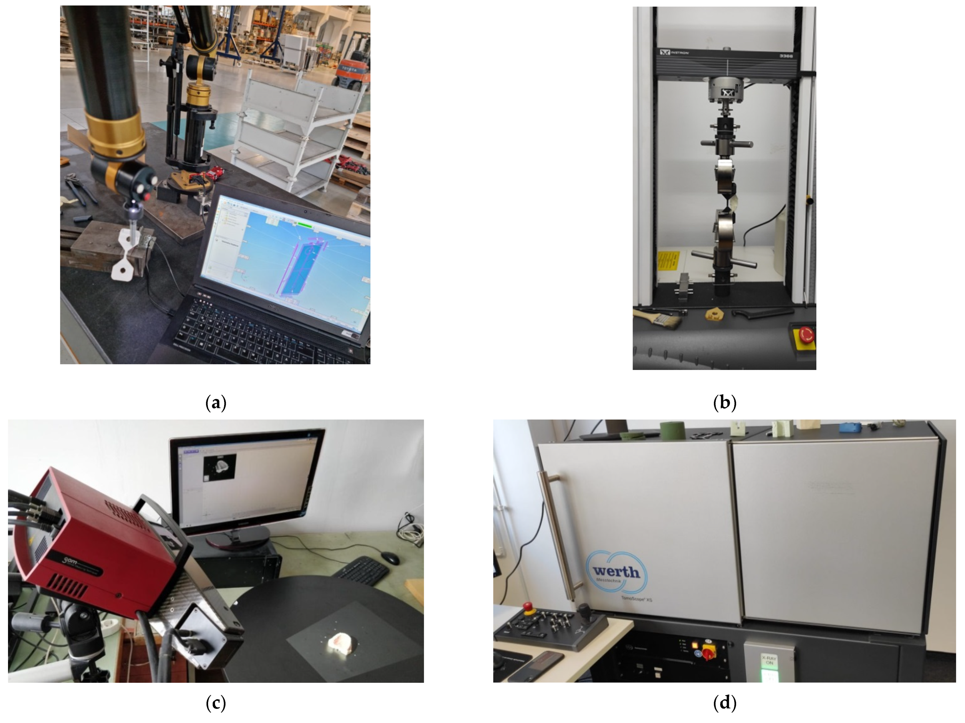
Dimensional and geometric measurements are performed using two main techniques, coordinate measuring and 3D scanning. High precision measurements are obtained using a Cimcore Stinger 2 [15] Coordinate Measuring Arm (Figure 4a) and Autodesk PowerInspect [16] software. Three-dimensional surface scan data is acquired using a Gom Atos II (Compact Scan) [17] structured light 3D scanner (Figure 4c). Computed Tomography data is acquired using a Werth XS Tomoscope [18] (Figure 4d), providing in-volume and surface 3D scans of the parts. Data obtained from optical 3D scans and computed tomography is used for CAD for actual mesh comparison using the Gom Inspect suite [19] software, providing a detailed analysis of geometric and dimensional deviations. These methods of measurement are chosen to provide as much detail as possible concerning dimensional and geometric characteristics of the manufactured parts, which are needed to guide decisions on how the input and output data should be chosen for ANN training as well as to provide information regarding the architecture of the ANN. Multiple points are sampled for each measured feature, and the results are averaged to reduce outliers and avoid sampling manufacturing artefacts such as holes or material overextrusion. Three-dimensional optical scans are used to corroborate results from CMM measurements and to provide details on surface topology and part warping. The ability to sample a large number of points for dimensional measurements using 3D scan data allows for better averaging of deviations and the eliminations or reduction of outliers caused over and under extrusion artefacts. Scans of the parts in the form of STL files can be used in the future for developing a more advanced neural network trained using printing parameters, CAD nominal model, and actual part 3D model.

Figure 4.
Machines used for performing measurements. (a) Cimcore Stinger 2, (b) Instron 3366, (c) GOM Atos II (CompactScan), (d) Werth Tomoscope XS.
Tensile strength measurements are performed on an Instron 3366 [20] tensile tester (Figure 4b). The data provided by these measurements can be used to model the mechanical behaviour of the manufactured parts, which can then be used to create an orthotropic material profile for CAD systems that can inform decisions of layer orientation and feature dimensions in the design stage, as well as provide data for the training of an ANN that can predict the mechanical behaviour of a part. The tests are performed on all test parts, and the results are plotted for pairs representing the horizontal and the vertical orientations for each combination of parameters, providing a comparative study of tensile strength for the different orientations used.
Artificial neural network development is performed using the Python [21] programming language through the PyCharm [22] Integrated Development Environment. To facilitate universality and cross-platform availability of the code, as well as to use various functions and tools optimised for machine learning, the neural network architectures are developed using the TensorFlow [23] machine learning library with the Keras [24] frontend. The architecture and performance of the tested neural networks are analysed using the TensorBoard [25] visualisation kit for TensorFlow. The performance analysis is displayed as a plot of ‘Training accuracy’ Vs. ‘Predictions on validation data’ accuracy in the form of the Mean Absolute Error (MAE) between predicted and actual values. A tendency of the MAE values to decrease indicates the ability of the model to learn the complex correlative function and the ability to generalise. The Mean Absolute Error metric is defined by Equation (1),
where MAE = Mean Absolute Error, yi is the prediction, xi is the true value, and “n” is the number of samples.
A base program is developed to create every neural network analysed in this study. The source code is written in the Python Programming language and is available for reference in Appendix A. The neural network is implemented as a Sequential Model inside the base program to facilitate the implementation of different model architectures. A neural network architecture in this context is defined by the number of layers and the number of nodes in every layer. A deep neural network (DNN) is defined as a neural network that contains multiple layers (also known as hidden layers) between the input and output layers. All of the neural networks analysed in this study are of the Deep Neural Network Type. Different architectures are developed by modifying the number of hidden layers and nodes in the sequential model implemented in the base program.
In the context of this paper, the neural network architecture will be defined as the number of hidden layers times the number of nodes per layer because all architecture will employ hidden layers with equal numbers of nodes; therefore, 3 × 32 indicates an architecture containing 3 hidden layers and 32 nodes per layer.
This study is performed on a number of neural networks composed of 2, 3, and 4 fully interconnected hidden layers containing 8, 32, and 64 nodes each, for a total of 9 architectures; thus, the number of weights (trainable parameters) is dependent on the number of nodes and the number of hidden layers used. The optimisers [26] used are Stochastic Gradient Descent and ADAdelta. The selection of the optimiser and the parameters for the optimiser (learning rate) is determined by observing the performance of the network under test (speed of convergence, accuracy of predictions). The weights and bias values of the neural networks are initiated as zeroes and adjusted by the optimiser during the training process. The number of hidden layers and nodes-per-layer are selected to represent networks with increasing parameter spaces (trainable parameters) in order to determine the optimal combination for best accuracy without overfitting the data. As the number of hidden layers and nodes-per-layer is highly dependent on the number of samples in the training dataset as well as the complexity of the problem to be solved, these parameters are subject to fine-tuning based on the observed performance of the network under test, as there is currently no clear mathematical formula for determining the exact architecture for a specific problem. The smallest network contains 2 hidden layers and 8 nodes per layer and is selected to provide a number of trainable parameters smaller than the number of samples in the present dataset and serves as a good starting point. The developed architectures are presented in Table 2 as well as the activation function for the hidden layers and the number of trainable parameters for each architecture.

Table 2.
Neural network architectures.
The number of epochs [27] for training the neural networks is not predetermined. The networks are allowed to train until they diverge or until the decrease in prediction error becomes insignificant.
Input and output layer shapes are determined by the number of input and output parameters, and the activation function for the output layer is Linear.
Strategies to prevent overfitting can be employed in the form of l2 regularisers [28] and Dropout layers [29] which can be implemented after each hidden layer. Dropout layers do not affect the number of trainable parameters and are employed only in architectures that show a tendency to overfit. The parameters for l2 regularisers and dropout layers are chosen by fine-tuning for best performance.
Separate neural networks are employed for predicting dimensional characteristics and mechanical characteristics. This modular approach allows for separate training of the neural networks according to the availability of data, while at the same time allowing for interconnectivity with other networks, i.e., the predictions for dimensional deviations and mechanical behaviour can be used as inputs for another network that can inform decisions on the best compromise between dimensional accuracy and mechanical properties.
The data used for training is provided in the form of comma separated values (CSV) tables containing both input and output data. The input data used for training the neural network employed for predicting dimensional deviations are in the form of the values for feature length, nozzle temperature, printing speed, orientation, material shrinkage rate, print cooling fan speed, and heated bed temperature. The material shrinkage rate is provided as a minimum, medium, and maximum shrinkage. The minimum and maximum shrinkage for PLA are 0.3% and 0.5%, and for PET-G 0.2% and 1% [30]. The medium shrinkage value is calculated as the average between the minimum and maximum values. The output data is in the form of deviations from the nominal dimension of the feature, the value of which is obtained through high precision metrology measurements. An example of the table head and a sample of values is presented in Table 3.

Table 3.
Sample of input data table head and values used for training dimensional characteristics neural network.
The neural networks employed in predicting mechanical properties have input data in the form of values for nozzle temperature, printing speed, material and orientation. The value for “material” represents categorical data; therefore, each material is encoded in the form of a number “1” for PETG and ”2” for PLA to avoid not a number (NaN) errors during training. Considering that for this dataset, the orientation also takes on only two values, horizontal and vertical, this feature is also encoded as a number “1” for horizontal and “2” for vertical. For datasets where the orientation takes on many different values, these can be provided as angles. The output data used for training the neural network are provided in the form of tensile strength values in [Mpa] obtained from tensile strength measurements. An example of a table head and a sample of values is presented in Table 4.

Table 4.
Sample of input data table head and values for training mechanical behaviour neural network.
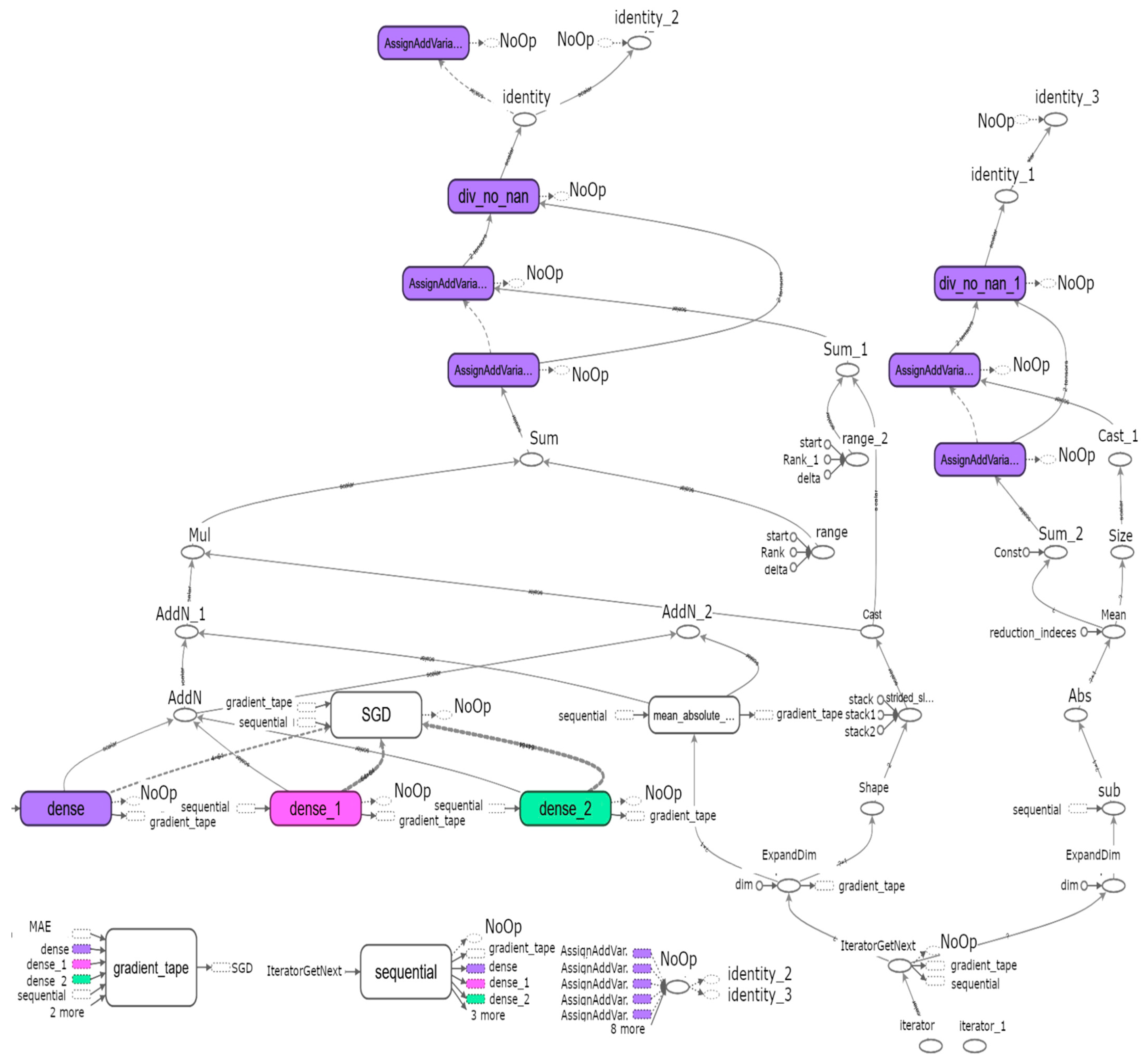
A graphical representation of a neural network analysed in this study showing the path of the data and the operations performed throughout the network during training is presented in Figure 5, showing the path of the data through the neural network. Data enters through the dense layers (dense, dense_1, dense_2), where an inference (prediction) is made. The result of the inference is used in combination with the actual value to compute the Mean Absolute Error (MAE). The error is used to adjust the value of the weights and biases to a degree determined by the optimiser employed, i.e., for Figure 5, the optimiser used is Stochastic Gradient Descent (SGD). The network design also employs functions to prevent NaN scenarios. The data is normalised (values scaled between 0 and 1) externally to allow for better portability of the model. Normalisation is performed to increase the speed of convergence by reducing the difference in scale between the various parameter values. Data normalisation is optional; however, it can increase model performance and decrease convergence times. The normalised data takes values from 0 to 1 but preserves the relative ratios between the original values.
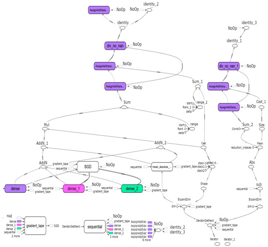
Figure 5.
Graphical representation of a neural network with 3 hidden layers.
4. Results
4.1. Part Measurement Results
Dimensional measurements provide the empirical data in the form of deviations from nominal feature length used to train the neural networks. The measurements are performed using two independent techniques, Coordinate measuring and 3D scanning, enabling cross-validation of data which can be used to eliminate outliers and reduce the noise inherent in any measurement process. Besides dimensional measurements, geometric analysis of the manufactured parts is very important for informing decisions regarding the selection of the training dataset. An in-depth analysis of the geometric and dimensional deviations of the manufactured parts indicates that material properties, in particular, material shrinkage rate, has a significant influence on the quality of the 3D printed components. Measurement results show that most of the deviations fall within the values predictable by the shrinkage rate of the material used, while the extent to which the parts deform due to this effect is influenced by nozzle temperature, print speed, and part cooling fan speed, parameters which influence layer and part cooling time directly. Analysis shows that parameter combinations that lead to short cooling times for the layers and the part, in general, tend to produce parts with higher dimensional and geometric deviations. This can be explained in part due to high internal tensions produced during rapid cooling that lead to more severe part warping and contraction. These results informed the decision of including material shrinkage rates and part cooling fan speed as training parameters for the artificial neural networks analysed in this study. Part warping can be analysed by performing a Surface comparison on CAD using data obtained from 3D scanning. Examples of severe part warping and mild part warping are presented in Figure 6, where (a) is the 230_60_H_PETG test part and (b) is the 220_45_H_PETG test part. The severity of part warping can be determined by the relative difference between the deviations of the part height along its full length, denoting the curvature of the part. The deviations in part height can be seen in the form of deviation labels in Figure 6. Measurement results for all manufactured parts show a high value for the deviation of the total length (130 mm) that can not be accounted for by the effects of contraction alone. Analysis of the effects of warping indicates that the high value for the deviation in total length is due to the curvature of the part. Therefore, a decision can be made regarding the inclusion of this specific feature length in the training data. The complete dimensional measurement results are found in Supplementary Materials Table S1.

Figure 6.
Surface comparison on CAD. (a) severe part warping, (b) mild part warping.
4.2. Tensile Strength Measurement Results
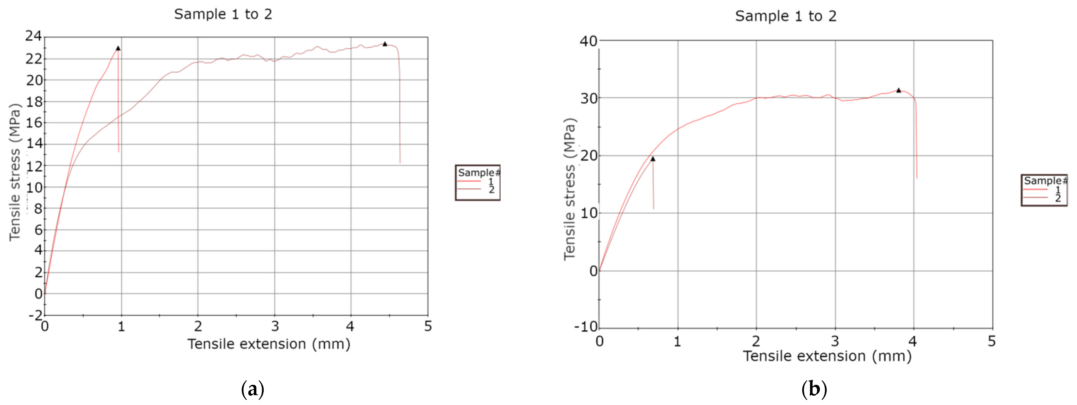
The results of tensile strength measurements are presented in Supplementary Materials Table S2 in the form of tensile stress at maximum load (at breaking point) expressed in [Mpa]. The plots of tensile strain vs. tensile stress for two pairs of test parts are presented in Figure 7, where (a) represents the test results for the pair composed of the 200_70_H_PETG and the 200_70_V_PETG part, while (b) represents the results for the pair composed of the 190_90_H_PLA part and the 190_90_V_PLA test part. Sample 1 represents horizontal part orientation and Sample 2 vertical part orientation. The results show that for the vertical orientation, the tensile strength is determined by layer adhesion, which is influenced by the temperature used during the manufacturing process; therefore, the results indicate that the tensile strength of parts manufactured in the vertical orientation is directly proportional to the nozzle temperature.
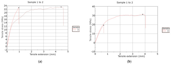
Figure 7.
Sample of tensile stress vs. tensile strain results. (a) 200_70_PLA pair, (b) 190_90_PLA pair.
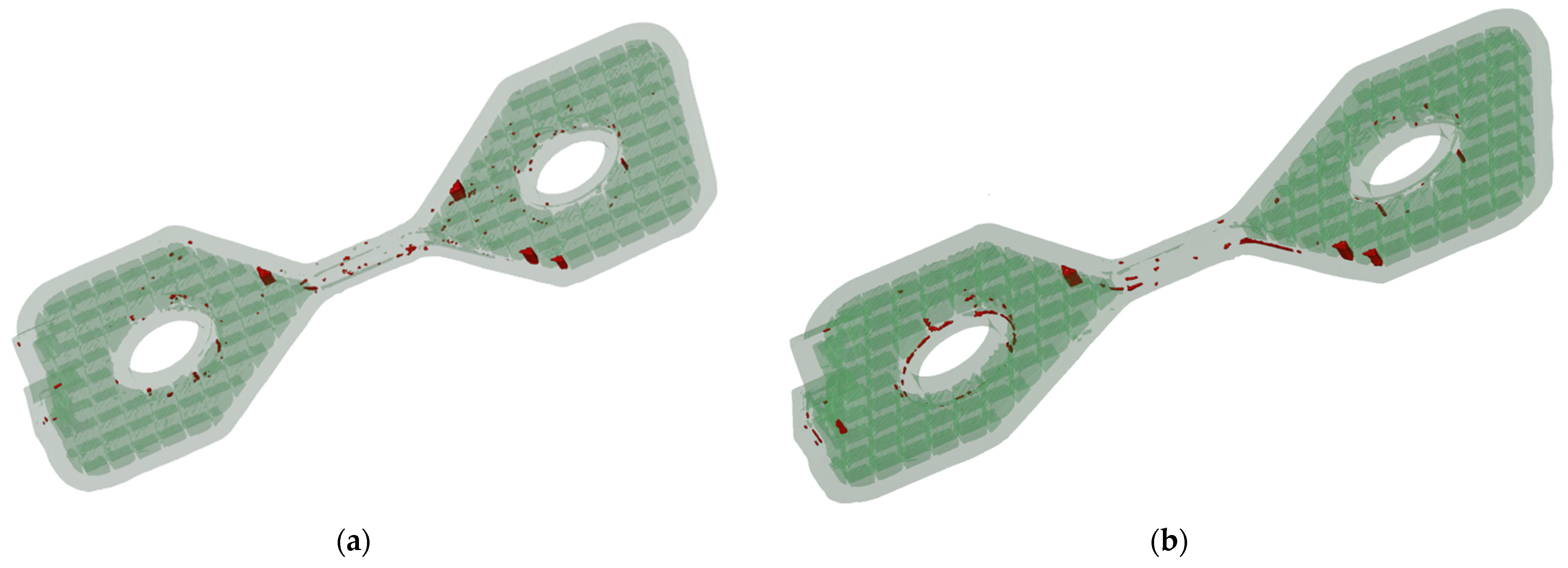
Tensile strength measurement results for test parts manufactured in the horizontal orientation show that, in this case, tensile strength is inversely proportional to temperature. This result can be explained by the increased porosity of parts manufactured at high temperatures and the thermal degradation of the material. An example of differences in porosity can be seen in Figure 8, where (a) is the 250_45_H_PETG part and (b) is the 220_45_H_PETG part. A higher porosity can be observed on the high-temperature part in the form of small holes in the volume of the material; however, although the low-temperature part presents a lower porosity, the effects of increased layer decohesion can be observed. These results must be taken into account when choosing manufacturing process parameters.

Figure 8.
The difference in porosity due to printing temperature. (a) high-temperature part (b) low-temperature part.
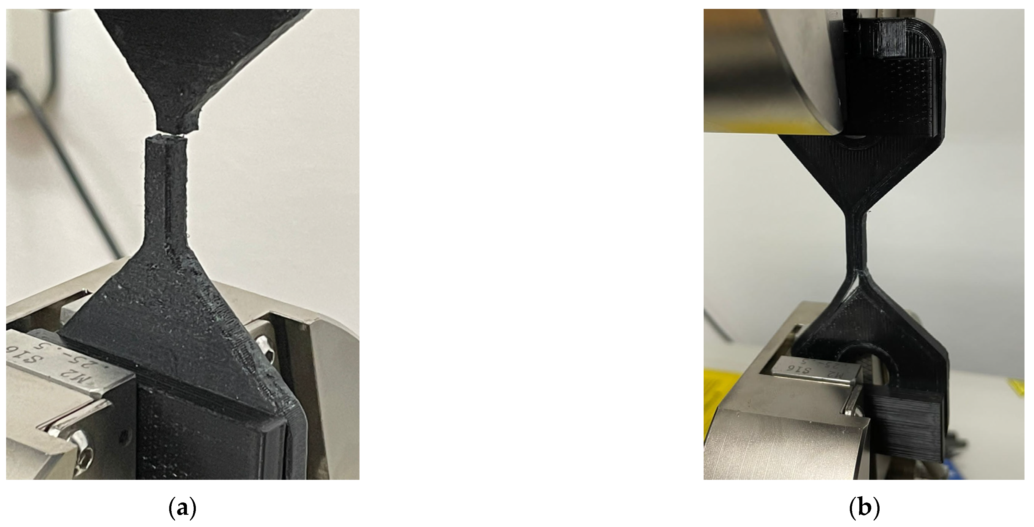
One reason for using a complex geometry test part is to determine the mechanical behaviour in scenarios closer to real-world cases. One such behaviour is the part failing in other areas than the designated failure zone before the part breaking. A comparison between a part breaking in the designated failure zone and a part that fails in other areas before breaking is shown in Figure 9. The part in Figure 9a represents expected behaviour, breaking in the designated failure zone. The part in Figure 9b presents the separation at the interface between the top and bottom layers and the part perimeter. This behaviour is accounted for by a low overlap percentage between the top/bottom layers and the part perimeter and is present for all materials tested (PETG and PLA). These results must be taken into account when choosing a top and bottom thickness and the overlap percentage. Another factor that influences this behaviour is infill pattern and density.
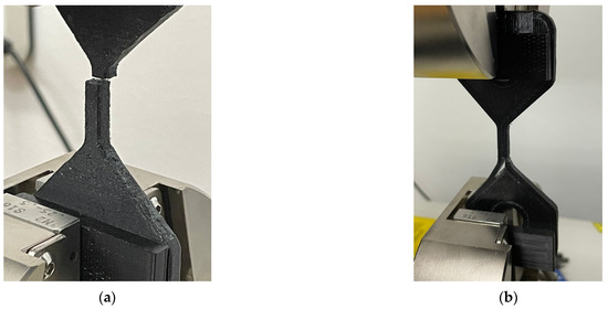
Figure 9.
Comparison of test part failure modes. (a) part breaking at designated failure point (b) part failing before breaking.
For training the neural network, only the data from parts breaking in the designated failure zone are used.
The results of dimensional and tensile strength measurements are presented in Table 5 in the form of deviations from nominal for dimensional measurements and maximum stress in MPa for tensile strength measurements. The maximum stress in MPa for parts that failed before breaking, as exemplified earlier and shown in Figure 9b, is also presented.

Table 5.
Dimensional and tensile strength measurement results.
4.3. Artificial Neural Network Performance Analysis Results
The performance of the tested ANN architectures is evaluated by plotting the Mean Absolute Error (MAE) of the training predictions versus the Mean Absolute Error of the predictions performed on the validation data. The validation data is not seen by the neural network during training and, at the same time, represents real-world data obtained by splitting the dataset between training and validation data, thus allowing an unbiased performance analysis applicable to real scenarios.
The interpretation of the plot is as follows: Two lines are plotted, one for training predictions and one for validation data predictions, as mentioned above. If the two lines show a tendency, however small of their respective mean absolute error, it indicates that the model can approximate a correlative predictive function for the input and output parameters and is also capable of generalising. If the lines show a tendency to diverge, i.e., the MAE of the training predictions decreases while the MAE of the validation data predictions increases, the model is considered to overfit the data, i.e., it starts to memorise data rather than approximate a predictive function. If the lines show a random distribution on the plot, this indicates that the model can not find a predictive function and a correlation between the input and output parameters.
A wide range of architectures was tested with 2 and 3 hidden layers and 8, 32, and 64 nodes per layer. The performance of each tested architecture is used to inform decisions regarding optimisation and fine-tuning of subsequent networks leading to an architecture that best fits the available dataset.
The performance plots for two architectures used for predicting tensile strength are presented in Figure 10. The architectures tested in the two plots are 3 × 64 and 3 × 32. From the plot, it can be seen that the model with the 3 × 64 tends to overfit the data. The best performance on the available dataset is reached by the model with 3 × 32 architecture. The performance plot for the 3 × 32 architecture shows good model generalisation and a tendency for the MAE to decrease; thus, the model shows the ability to learn a correlative and predictive function using the input and output parameters provided. Due to the low number of parameters and strong correlation between them, the neural network for predicting tensile strength is able to approximate a predictive function in a short time on a lower number of nodes, while at the same time, the low number of parameters leads to overfitting on large models.

Figure 10.
Performance plots for tensile strength predictive models. (a) 3 × 64 architecture, (b) 3 × 32 architecture.
Performance plots for dimensional deviation predictive models are presented in Figure 11. Due to the increased complexity of the problem that needs to be solved for this model and the high number of input parameters, a larger model is required to approximate a correlative and predictive function. Because of the low performance of 3 × 8 and 3 × 32 architectures, a 4 × 64 architecture was also analysed for performance to provide a comparison point for the 3 × 64 architecture. An analysis of the plots shows that the model with 4 × 64 architecture tends to overfit the data. The best performance was achieved by the model with 3 × 64 architecture, showing a tendency to reduce the Mean Absolute Error for both the training and validation data predictions. Due to the high complexity of the problem to be solved by the model and the high number of input parameters, the predictive model for dimensional deviations takes longer times to train than the simpler model for predicting tensile strength. However, the model reached a value of 0.05 for the mean absolute error of the predictions for validation data after 120,000 training epochs [23] while still showing a tendency to improve. A value of 0.05 for MAE is insignificant; therefore, the model can produce usable predictions.

Figure 11.
Performance plots for dimensional deviation predictive models. (a) 4 × 64 model architecture (b) 3 × 64 model architecture.
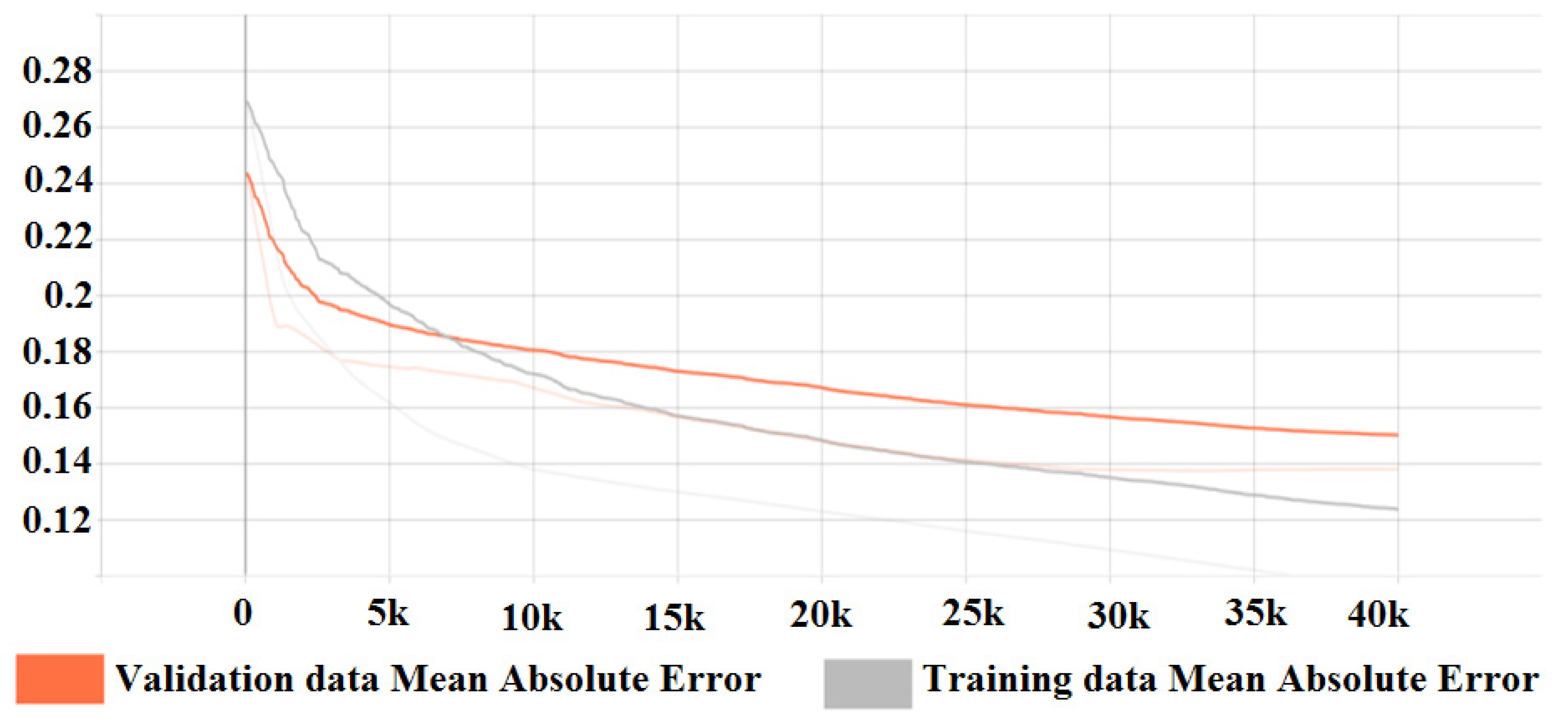
The neural networks can be optimised for better generalisation and performance by choosing adequate optimisers [24], increasing the number of layers and nodes, and implementing techniques such as layer weight regularisation [25] and dropout layers [26]. The input data needs to be curated as well, outliers need to be eliminated, and input parameters with low variety should also be eliminated; otherwise, the neural network will consider them as categorical data. An example of this behaviour can be observed in the data for shrinkage, cooling fan speed, and bed temperature. These parameters have only two values in the dataset. For large datasets that are comprised of parts manufactured from more materials at a variety of printed bed temperatures and cooling fan speed, these parameters can be accounted for and included. A performance plot for an optimised neural network is presented in Figure 12. The neural network employs the Adadelta optimiser and techniques to prevent overfitting. The parameters with a low variety were removed, and training was performed strictly on the main process parameters, temperature, speed and feature length. The plot indicates that the model can generalise, with both MAE values tending to decrease.
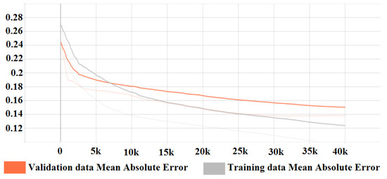
Figure 12.
Performance plot for an optimised neural network with 3 × 64 architecture.
5. Discussion
The study shows that predicting dimensional deviations and mechanical behaviour in the form of tensile strength is feasible. The ability of the model to generalise is dependent on the quantity, quality, and variety of the input data. The dataset used in this study is limited, however, it is sufficient to prove that predictive models can be created, encouraging future research on large datasets. The models present predictions with higher accuracy than the predictions obtained through linear regression in previous studies. The predictions provided by the models can be used for guiding decisions regarding the choice of parameters for manufacturing and for compensating dimensional deviations in the design phase, leading to a lower number of failed parts and the reduction or elimination of postprocessing operations.
The findings are consistent with the results of previous studies in the field.
The inclusion of additional parameters such as shrinkage rate, printing speed, part fan cooling speed, and heated bed temperature as input training data does not diminish the neural network’s ability to learn and approximate the predictive function, indicating that a correlation exists between these parameters and dimensional deviations. However, the dataset needs to be improved in variety and quantity for these parameters to be statistically significant and to increase prediction accuracy. An absolute minimum of three different values for each of the parameters must be used, i.e., three different materials, three different heated bed temperatures, etc.
The study shows a strong correlation between parameters that affect part and layer cooling times and dimensional deviations. Therefore, ambient temperature plays an important role; however, the study was performed under controlled laboratory conditions of constant temperature and humidity; thus, future datasets must include environmental variables such as ambient temperature and relative humidity.
The neural networks developed in this study can be used to provide predictions in the form of dimensional deviation or tensile strength of a part for a given parameter combination or for determining the best parameter combination for a given dimensional deviation or tensile strength value by reversing the input and output configuration of the model. The predicted values for dimensional deviations can be used to adjust a parametric CAD model of the part to compensate for the errors. The predicted tensile strength values can guide decisions for optimal part orientation and manufacturing parameter selection. However, while the networks developed for this study provide simple predictions of deviations and tensile strength that can be used in real-world applications for improving part quality and mechanical behaviour, the main utility of these networks is for informing the development of more complex networks or as modules in interconnected network designs.
6. Conclusions
The results show that artificial neural networks are capable of learning complex predictive functions for the quality of FDM manufactured parts, encouraging and informing future work in the field.
The limiting factors were determined to be the size and variety of the available dataset on which the performance of the neural networks depends; therefore, the authors propose the creation of an open public database where individuals and institutions can submit and access measurement data on additive manufactured parts in the form of 3D scans, high precision metrology, and tensile strength measurements.
Guided by the findings of this study and the ability of artificial neural networks to approximate and learn complex functions and to work on large datasets and input data, a future study is proposed to develop a neural network that takes the point cloud, or STL file of an FDM manufactured part and the process parameters as input and provides, as output, a compensated STL file, using the predictions to modify the coordinates of the points which define the 3D model. Such a network will most probably be in the form of a generative model, i.e., a Generative Adversarial Neural network or a Variational Autoencoder.
Supplementary Materials
The following supporting information can be downloaded at: https://www.mdpi.com/article/10.3390/machines10020128/s1, The data used for training the neural networks is published alongside the manuscript in the form of tables, Table S1: Dimensional training data, Table S2: Tensile strength training data.
Author Contributions
Conceptualization, S.D.G., A.D.S. and V.C.; methodology, S.D.G., A.D.S. and V.C.; software, A.D.S.; validation, S.D.G. and V.C.; formal analysis, S.D.G., A.D.S. and V.C.; investigation, S.D.G., A.D.S. and V.C.; resources, S.D.G. and V.C.; data curation, A.D.S.; writing—original draft preparation, A.D.S.; writing—review and editing, M.K., M.P., V.C. and A.D.S.; visualization, A.D.S.; supervision, S.D.G.; project administration, V.C.; funding acquisition, S.D.G. All authors have read and agreed to the published version of the manuscript.
Funding
This research was funded by the Technical University of Cluj-Napoca, and The APC was funded by the Technical University of Cluj-Napoca.
Acknowledgments
Special thanks to our colleagues at the Technical University of Cluj-Napoca, Eugen GUTIU for manufacturing the test parts, Assoc. Prof. Pop GRIGORE for providing high precision metrology measurements, Vlad BOCANET for providing 3D scans. High precision metrology measurements were also provided through a collaboration with the Technical University of Vienna facilitated by the CEEPUS program and the OeAD. Special thanks go to the team from TU-WIEN: Numan M. Durakbasa, Osman BODUR and Res. Assist. Eva Maria WALCHER. Computer Tomography measurements were made possible by collaborating with the Werth Messtechnik Österreich GmbH company.
Conflicts of Interest
The authors declare no conflict of interest.
Appendix A
import pandas as pd
from time import time
from keras import backend as K
from sklearn import preprocessing
from keras.layers import Dropout
from keras import regularizers
from tensorflow.python.keras.callbacks import TensorBoard
from keras.callbacks import ModelCheckpoint
import tensorflow as tf
from tensorflow.keras import layers
from sklearn.model_selection import train_test_split
printed_train = pd.read_csv("force train.csv",names=["temp", "speed", "material", "orientation", "mpa"], skiprows=1)
datasetf = printed_train.values
x = datasetf[:, 0:4]
y = datasetf[:, 4]
min_max_scaler = preprocessing.MinMaxScaler()
xs = min_max_scaler.fit_transform(x)
xt, xv, yt, yv = train_test_split(xs, y, test_size=0.1, shuffle=True)
printed_model = tf.keras.Sequential([
layers.Dense(64,kernel_regularizer=regularizers.l2(0.001),activation='relu',input_shape=(4,)),
layers.Dropout(0.2),
layers.Dense(64, kernel_regularizer=regularizers.l2(0.001),activation='relu'),
layers.Dropout(0.1),
layers.Dense(64,kernel_regularizer=regularizers.l2(0.001), activation='relu'),
layers.Dropout(0.1),
layers.Dense(1, activation='linear')
])
tensorboard = TensorBoard(log_dir="logs/{}".format(time()))
printed_model.compile(loss=tf.keras.losses.MeanAbsoluteError(),optimizer=tf.optimizers.SGD(0.01),metrics=[tf.keras.metrics.MeanAbsoluteError()])
checkpoint = ModelCheckpoint("best_model_valforce.hdf5", monitor='val_mean_absolute_error', verbose=1,save_best_only=True, mode='min')
earlystop=tf.keras.callbacks.EarlyStopping(monitor='val_mean_absolute_error',mode='min', min_delta=1, patience=2000),
printed_model.fit(xt, yt, epochs=30000, shuffle=True, validation_data=(xv, yv),
callbacks=[checkpoint,earlystop, tensorboard]).
References
- Bodur, O.; Stepanek, V.; Walcher, E.M.; Durakbasa, N. Precision in additive manufacturing optimization and evaluation of the accuracy of 3D printer based on GPS system. In Proceedings of the 31st DAAAM International Symposium, Mostar, Bosnia and Herzegovina, 21–24 October 2020; Katalinic, B., Ed.; DAAAM International: Vienna, Austria, 2020; pp. 0963–0972, ISBN 978-3-902734-29-7. [Google Scholar] [CrossRef]
- Yadav, D.; Chhabra, D.; Garg, R.K.; Ahlawat, A.; Phogat, A. Optimization of FDM 3D printing process parameters for multi-material using artificial neural network. Mater. Today Proc. 2020, 21, 1583–1591. [Google Scholar] [CrossRef]
- Deshwal, S.; Kumar, A.; Chhabra, D. Exercising hybrid statistical tools GA-RSM, GA-ANN and GA-ANFIS to optimize FDM process parameters for tensile strength improvement. CIRP J. Manuf. Sci. Technol. 2020, 31, 189–199. [Google Scholar] [CrossRef]
- Mohamed, O.A.; Masood, S.H.; Bhowmik, J.L. Modeling, analysis, and optimization of dimensional accuracy of FDM-fabricated parts using definitive screening design and deep learning feedforward artificial neural network. Adv. Manuf. 2021, 9, 115–129. [Google Scholar] [CrossRef]
- Tura, A.D.; Mamo, H.B.; Jelila, Y.D.; Lemu, H.G. Experimental investigation and ANN prediction for part quality improvement of fused deposition modeling parts. IOP Conf. Ser. Mater. Sci. Eng. 2021, 1201, 012031. [Google Scholar] [CrossRef]
- Lyu, J.; Manoochehri, S. Dimensional Prediction for FDM Machines Using Artificial Neural Network and Support Vector Regression. In Proceedings of the International Design Engineering Technical Conferences and Computers and Information in Engineering Conference, Anaheim, CA, USA, 18–21 August 2019. [Google Scholar] [CrossRef]
- Sterca, A.D.; Calin, R.A.; Cristian, L.; Walcher, E.M.; Bodur, O.; Ceclan, V.; Grozav, S.D.; Durakbasa, N.M. Evaluation of Fused Deposition Modeling Process Parameters Influence on 3D Printed Components by High Precision Metrology. In Digitizing Production Systems; Lecture Notes in Mechanical Engineering; Durakbasa, N.M., Gençyılmaz, M.G., Eds.; Springer: Cham, Switzerland, 2022. [Google Scholar] [CrossRef]
- Understand Neural Networks & Model Generalization, Towardsdatascience.com. Available online: https://towardsdatascience.com/understand-neural-networks-model-generalization-7baddf1c48ca (accessed on 27 December 2021).
- Dassault Systems SolidWorks. Available online: https://www.solidworks.com/domain/design-engineering (accessed on 27 December 2021).
- ISO 1101. Geometrical product specifications (GPS)—Geometrical tolerancing—Tolerances of form, orientation, location, and run-out. 2017. Available online: https://www.iso.org/obp/ui/#iso:std:iso:1101:en (accessed on 10 January 2022).
- DevilDesign PET-G Product Description. Available online: https://devildesign.com/download/PET-G_-_product_card.pdf (accessed on 27 December 2021).
- DevilDesign PLA Product Description. Available online: https://devildesign.com/download/PLA_-_product_card.pdf (accessed on 27 December 2021).
- AnyCubic 4Max Pro 2.0. Available online: https://www.anycubic.com/products/4max-pro-2-0 (accessed on 27 December 2021).
- Leapfrog Creatr HS User Manual. Available online: http://support.lpfrg.com/support/solutions/articles/11000083231-user-manual (accessed on 27 December 2021).
- Hexagon Manufacturing Intelligence Coordinate Measuring Arms. Available online: https://www.hexagonmi.com/?utm_source=DomainRedirect&utm_medium=cimcore (accessed on 27 December 2021).
- Autodesk PowerInspect. Available online: https://www.autodesk.com/products/powerinspect/overview (accessed on 27 December 2021).
- Gom Atos II (Compact Scan). Available online: https://www.gom.com/en/products/3d-scanning/atos-compact-scan (accessed on 27 December 2021).
- TomoScope®XS, Werth, Inc. 2018. Available online: http://werthinc.com/products/tomoscope-xs/ (accessed on 27 December 2021).
- GOM Inspect Suite. Available online: https://www.gom.com/en/products/gom-suite/gom-inspect-pro (accessed on 27 December 2021).
- Instron 3360 Series Mechanical Testing Systems. Available online: https://www.instron.com/~/media/literature-library/products/2011/06/3300-series-table-model.pdf (accessed on 27 December 2021).
- Python Programming Language. Available online: https://www.python.org/ (accessed on 27 December 2021).
- PyCharm Integrated Development Environment. Available online: https://www.jetbrains.com/pycharm/ (accessed on 27 December 2021).
- TensorFlow Machine Learning Platform. Available online: https://www.tensorflow.org/ (accessed on 27 December 2021).
- Keras Frontend for TensorFlow. Available online: https://keras.io/ (accessed on 27 December 2021).
- TensorBoard Visualisation Kit for TensorFlow. Available online: https://www.tensorflow.org/tensorboard (accessed on 27 December 2021).
- An Overview of Gradient Descent Optimization Algorithms. Available online: https://ruder.io/optimizing-gradient-descent/ (accessed on 29 December 2021).
- Epoch Definition. Available online: https://deepai.org/machine-learning-glossary-and-terms/epoch (accessed on 27 December 2021).
- Layer Weight Regularizers. Available online: https://keras.io/api/layers/regularizers/ (accessed on 29 December 2021).
- Dropout Layer. Available online: https://keras.io/api/layers/regularization_layers/dropout/ (accessed on 29 December 2021).
- Shrinkage Values for Different Plastic Materials. Available online: https://omnexus.specialchem.com/polymer-properties/properties/shrinkage (accessed on 27 December 2021).
Publisher’s Note: MDPI stays neutral with regard to jurisdictional claims in published maps and institutional affiliations. |
© 2022 by the authors. Licensee MDPI, Basel, Switzerland. This article is an open access article distributed under the terms and conditions of the Creative Commons Attribution (CC BY) license (https://creativecommons.org/licenses/by/4.0/).

