Dynamic System Modeling of a Hybrid Neural Network with Phase Space Reconstruction and a Stability Identification Strategy

Abstract

Focusing on the identification of dynamic system stability, a hybrid neural network model is proposed in this research for the rotating stall phenomenon in an axial compressor. Based on the data fusion of the amplitude of the spatial mode, the nonlinear property is well characterized in the feature extraction of the rotating stall. This method of data processing can effectively avoid the inaccurate recognition of single or multiple measuring sensors only depending on pressure. With the analysis on the spatial mode, a chaotic characteristic was shown in the development of the amplitude with the first-order spatial mode. With the prerequisite of revealing the essence of this dynamic system, a hybrid radial basis function (RBF) neural network was adopted to represent the properties of the system by artificial intelligence learning. Combining the advantages of the methods of K-means and Gradient Descent (GD), the Chaos–K-means–GD–RBF fusion model was established based on the phase space reconstruction of the chaotic sequence. Compared with the two methods mentioned above, the calculation accuracy was significantly improved in the hybrid neural network model. By taking the strategy of global sample entropy and difference quotient criterion identification, a warning of inception can be suggested in advance of 12.3 revolutions (296 ms) with a multi-step prediction before the stall arrival.

1. Introduction

As one of the most difficult problems in dynamic system stability, the rotating stall phenomenon seriously restricts the performance and operation safety of the compressor. After the idea of active control for the stall in compressors proposed by Epstein [1], two recognized stall types were reported by researchers. McDougall [2] and Day [3] first discovered the pre-stall inception as the modal wave and the spike wave. Paduano [4] divided the development of the rotating stall in the compressor into four stages in detail, namely as the pre-stall, the initial disturbance stage of the rotating stall, the complete stall stage and the surge stage. Considering the importance of identifying stall precursors in advance, a lot of effort has been made in terms of signal recognition.

The cross-correlation analysis on the measured pressure signals was performed by Tahara [5]. It was found that as the stall approached, the correlation decreased significantly. A variance method was used by Liu [6] to detect the precursor signal of instability in the compressor. Then, an embedded early warning system was developed for rotating stall recognition. An alarm can be given about 20 ms and 80 ms before the stall arrival, for the instability of spike-types and modal wave-types, respectively. Cameron [7] summarized the application of the visual inspection method, spatial Fourier analysis and the wavelet transform method in stall initiation detection. Moreover, a new method was proposed based on a windowed two-point correlation function with adjacent sensors. The features of disturbances were highlighted at the beginning of the stall with a certain spatial and temporal resolution. The fast wavelet technique was employed by Liu [8] to predict the stall inception of an axial compressor. By reasonably selecting the reconstruction frequency, these two kinds of stall inception can be predicted in advance. Although the aerodynamic system stability of compressors has been studied for years, challenges and difficulties for the initial stall detection still exist.

The triggering of stall initiation is a complex system process, including the mechanism of flow mechanics and aerodynamic systems. It is very difficult to predict the rotating stall behavior. With the rapid development of artificial intelligence learning technology, it is feasible to look for an intelligent method to build the model of the dynamic system and predict the occurrence of rotating stall in compressors. Machine learning algorithms have the ability of processing multi-dimensional data sets in a wide range, and can establish a connection between complicated nonlinear behaviors that cannot be identified by other means. Once the relationship is recognized by the algorithm, the outcome can be predicted based on the input provided. In recent years, machine learning algorithms have gradually been applied to the study of system identification.

With the procedure of phase space transformation in the extraction of signal features, the prediction on the rotating stall in a centrifugal fan was performed by Xu [9] by using a support vector regression machine (SVRM) as the regression model. The detection of stall inception was captured in advance of five steps in the basis of wavelet analysis. With the high-order Moore–Greitzer model, an initial disturbance recognition method was proposed by Wang [10,11] based on deterministic learning theory and a dynamic mode recognition method. Samuel [12] used the method of long short-term memory (LSTM) in the training of the stall dataset in compressors, and the classification and regression methods were adopted to model the neural network. After comparing the performances of the neural networks on predictability, the position of stall inception was predicted by threshold logic. The results showed that the regression method based on the LSTM model could predict the occurrence of a rotating stall for 5–20 ms in advance.

At present, the research on the rotating stall mostly depends on the simplification and assumption of ideal behavior and its physical model. With the development of artificial intelligence technology, the application of machine learning on fluid mechanics has been explored. However, only a few studies have been reported to establish the model of rotating stall phenomenon by machine learning, and most of them are aimed at methods rather than the physical phenomena. Therefore, this research intends to analyze the pressure signal characteristics of the casing wall and extract the circumferential pressure pulsation traveling wave to reflect the aerodynamic stability of the compressor. Through the discrete Fourier transform (DFT), the amplitudes of circumferential spatial modes can be obtained during the development of the rotating stall. So, the process of aerodynamic stability in the compressor can be accurately reflected by the variation of the amplitude with circumferential spatial modal. Under this circumstance, a Chaos–K-means–GD–RBF hybrid neural network model is proposed in this paper. Compared with the single method as mentioned above, the fusion algorithm not only has the advantage of a high calculation accuracy, but also improves the calculation efficiency significantly. According to the prediction of the established intelligent model, the sample entropy algorithm is carried out to identify the stall precursor. The aim of this proposed fusion model is to provide a new insight for the intelligent recognition and early warning of the rotating stall in compressors.

The organization of this paper is given as follows. Firstly, the original data collected in the experiment are preprocessed. The amplitude of the first-order spatial mode is calculated to characterize the process of the rotating stall in the compressors. Next, the chaotic performance of the spatial modal in time series is analyzed to lay a theoretical foundation for the subsequent modeling. On this basis, a Chaos–K-means–GD–RBF neural network fusion model is proposed to predict the stability of the dynamic system through model comparison. Finally, based on the established hybrid model, the amplitude of spatial modal is predicted by the single-step and multi-step, respectively. Moreover, the identification on the stall precursor is achieved with the sample entropy algorithm, as well as the difference quotient criterion.

2. Analytical Process of Data Characterization

2.1. Preprocessing of Initial Dataset

The experimental object in this paper is a low-speed single-stage axial compressor with a design speed of 3000 rpm. It consists of a stage with 19 rotor blades and 13 stator blades with the C4 profile. The schematic diagram of the compressor experiment and the location of the pressure sensors are shown in Figure 1. The Reynolds number is about 2 × 10⁵ based on rotor tip chord. The main geometric and aerodynamics parameters concerning the compressor stage are listed in

Table 1. Main design parameters of compressor.

Parameter	Value
Design speed n (rpm)	3000
Outer diameter D (mm) Tip speed (m/s)	450 70.7
Hub-tip ratio	0.75
Rotor blade number	19
Stator blade number	13

. A detailed introduction of the compressor is presented in Zhang [13]. Through the establishment of a high-speed data acquisition system, the dynamic pressure data of five measuring sensors were collected, which were uniformly located at the leading edge of the rotor blade on the casing in a circumferential direction (Figure 1a).

The original output voltage signal at measuring point #1 was obtained in Figure 2 at the rotating speed of 2500 rpm. Because of the noise signal in the collected data, it was necessary to carry out a low-pass filter processing on the original signal to filter out the high frequency noise. Then, the voltage signal could be converted into the pressure data through a linear transformation. In this paper, data sampling was performed at a sampling frequency of 5000 Hz. As to improve the computational efficiency, on the premise of ensuring signal with no distortion, the sampling time was changed to increase the time interval of the sequence. According to the Nyquist sampling theorem, the pressure signal data after the low-pass filtering was resampled to reach a sampling rate of 500 Hz. The sampling factor was chosen to be 10.

In the denoise procedure, wavelet decomposition and reconstruction technology are adopted in this article. Figure 3 shows the pressure data of each measuring point in time domain after resampling and denoising. It can be seen from the Figure 3 that under normal working conditions, the pressure signal of each measuring point was relatively stable. However, the pressure of each measuring point fluctuated greatly as the working state of the compressor approached the stall boundary. The stall wave propagated along the circumferential direction of the compressor, corresponding to the loss of stability in the dynamic system.

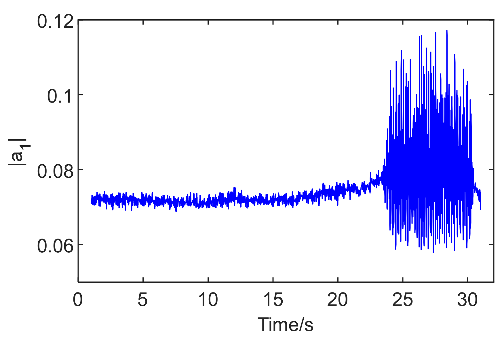
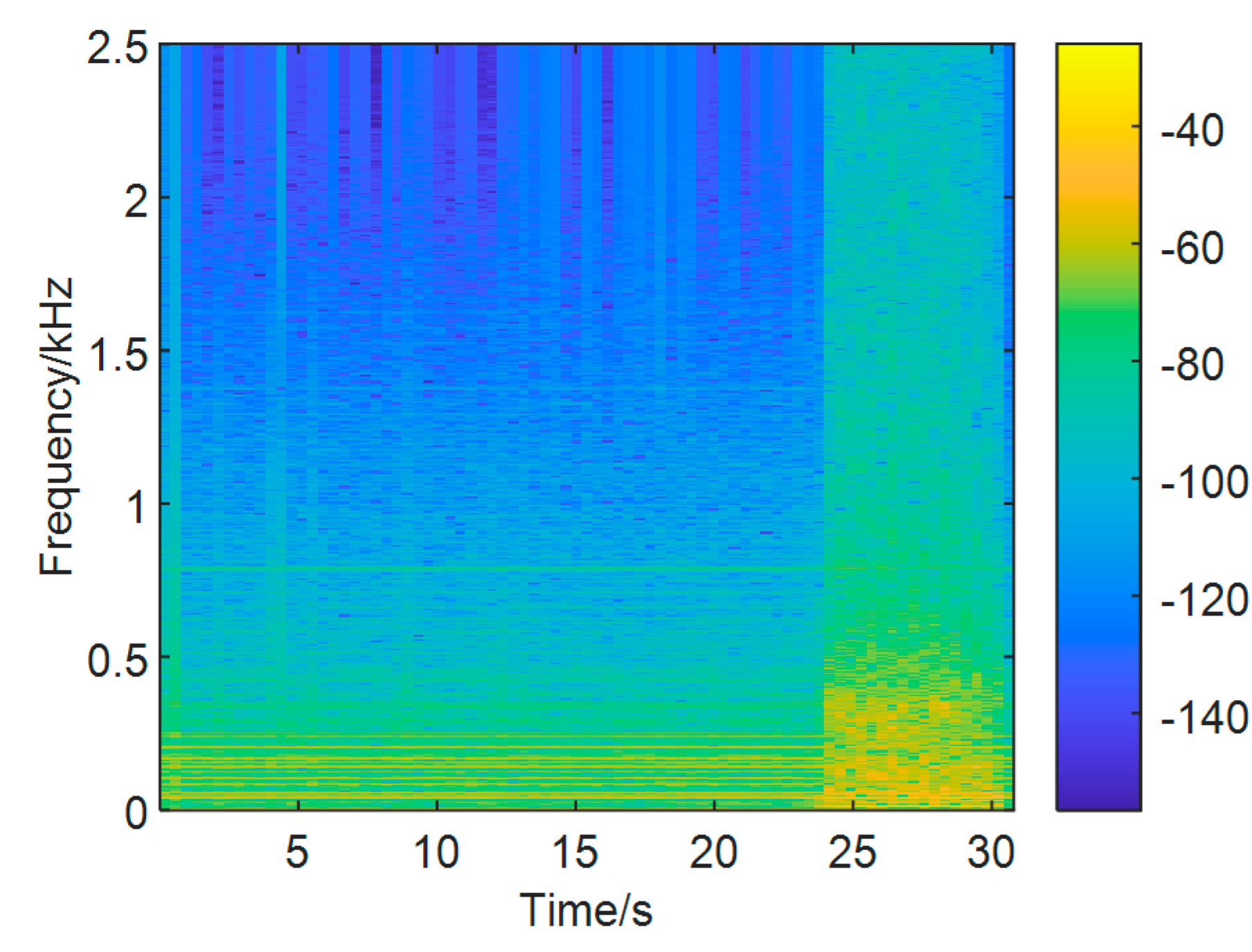
2.2. Feature Extraction of the Spatial Mode

In order to establish an accurate rotating stall prediction model, the pressure data of all measuring points were fused into an aggregation. The process of the rotating stall in the system was presented by the variation of modal wave energy, which reflects the essence and physical characteristics of the system. In the development of the rotating stall, the stall microcells can be expanded into the superposition of multiple harmonics. The amplitude of each traveling wave was extracted by discrete Fourier transform (DFT). Then, the amplitude of the k-th circumferential mode was obtained during the development of the stall cells, which is described in reference [14]. The expression of k-th spatial mode is defined as Equation (1):

$$a_k=\frac{1}{V} {\displaystyle \sum _{v=1}^V{\mathrm{\Phi }}_v{e}^{-2\pi ikv/V}},$$

(1)

where $V$ is the number of dynamic pressure sensors, and ${\mathrm{\Phi }}_v$ represents the flow coefficient converted from the dynamic pressure of the sensors.

The flow coefficient ${\mathrm{\Phi }}_v$ is obtained by Bernoulli’s equation, and its expression is indicated in Equation (2):

$${\mathrm{\Phi }}_v=\frac{\sqrt{2\left|P_a-P_v\right|/\rho }}{U}, U=2\pi Rf,$$

(2)

where $P_a$ is the atmospheric pressure, $P_v$ is the static pressure of the casing measured by the sensor, $\rho$ is the atmospheric density, $R$ is the average radius of the rotor, and $f$ is the rotor frequency.

According to the pressure signals after resampling and denoising, the first-order spatial mode amplitude |a1| in the development of the rotating stall is shown in Figure 4. This method of data processing can effectively avoid the inaccurate recognition of the single or multiple measuring sensors only depending on pressure. It can be seen that the amplitude of the first-order spatial mode fluctuated sharply, corresponding to the large fluctuation of pressure in Figure 3. From the analysis on the frequency diagram of the amplitude of spatial mode calculated in Figure 5, it can be concluded that the moment with the characteristic frequency of the stall cell concentrated was consistent with the moment of the amplitude of the spatial mode in the large fluctuation. The time of entering stall was calculated to be at about 23.97 s. The variation of the first-order spatial modal amplitude accurately reflects the basic features of the dynamic system in the compressor from normal operating conditions to the rotating stall condition. In the stage of neural network modeling, the amplitude of the first-order spatial mode in time series will be employed to establish a system stability prediction model.

2.3. Chaotic Characteristics of Spatial Mode with Time Series

2.3.1. Phase Space Reconstruction of Spatial Mode

Any variable data with time series in the system always contains the information of all variables with long-term evolution in the system. In actual engineering problems, the information of a one-dimensional data format in time series is usually common. Therefore, the reconstruction of the dynamic system from this one-dimensional data format is important to extract the relevant information needed.

According to the Takens theorem, in a multi-dimensional phase space composed of a one-dimensional observation sequence and its appropriate delay time, the dynamic behavior with system evolution can be expressed by the evolution trajectory of the points in the space with non-singularity [15]. The space composed of the observations and its delay time is called the reconstructed phase space. The delay vector technique is commonly used in the phase space reconstruction method.

Set a(1), a(2),…a(n) as the one-dimensional spatial mode amplitude obtained by denoising and DFT from the pressure signal, and reconstruct the phase space as follows:

$$\left\{\begin{array}{c}{X}_1=[a(1),a(1+\tau ),a(1+2\tau ),\cdots ,a(1+(m-1)\tau )]\\ X_2=[a(2),a(2+\tau ),a(2+2\tau ),\cdots ,a(2+(m-1)\tau )]\\ ⋮\\ X_n=[a(n),a(n+\tau ),a(n+2\tau ),\cdots ,a(n+(m-1)\tau )]\end{array}\right.,$$

(3)

where n = N − (m − 1)$\tau$, N is the total number of signal data points, m is the embedding dimension, $\tau$ is the delay time, and $X_i$ (i = 1, 2, …, n) is the delay vector.

2.3.2. Chaotic Determination of Spatial Mode

In this section, by calculating the best delay time $\tau$ for spatial mode amplitude |a1| in the time series, and the best embedding dimension m, the paper introduces the largest Lyapunov exponent of the sequence as the standard to identify systemic running state. Through the quantitative analysis, it is determined that the spatial modal amplitude |a1| with time series is a chaotic sequence, which provides a theoretical basis for the modeling of chaotic time series. The reconstruction delay time $\tau$ and the embedding dimension m are required in the procedure of phase space reconstruction. The selection of these two reconstruction parameters directly affects the similarity between the reconstructed phase space and the original system. In this paper, the Average Mutual Information function (AMI) [16] and the False Nearest Neighbors function (FNN) [16] are used to determine the two important parameters. The Average Mutual Information can be considered a nonlinear generalization of the autocorrelation function, expressed as:

$$I(x(t),x(t+\tau ))={\displaystyle \sum _{i,j}{p}_{ij}(\tau )\log (\frac{p_{ij}(\tau )}{p_i{p}_j})},$$

(4)

Here, $p_i$ is the probability that x(t) is in bin i of the histogram constructed from the data points in x, and $p_{ij}(\tau )$ is the probability that x(t) is in bin i and x(t + $\tau$) is in bin j.

In the computation on delay time $\tau$ by the average mutual information function, the tendency of the correlation function with the delay time is indicated in Figure 6a. As the literature [16] pointed out, the minimum value of function I($\tau$) indicates the maximum uncorrelated possibility of x(n) and x(n + $\tau$). The first minimum value of I($\tau$) is chosen as the optimal delay time during phase space reconstruction. However, in practice, There may be not a local minimum in I($\tau$), but a monotonic decreasing function. Therefore, the selection of the parameter needs to be formulated in combination with another standard. In this solution, the value of $\tau$ which is lower than the value 1/e in the AMI function, is selected as the optimal delay time. Under this condition, the optimal delay time $\tau$ is obtained as 8 in the time series of spatial modal amplitude |a1| according to the average mutual information function in this research.

Figure 6b shows the variation of the proportion of false nearest neighbor points with the embedding dimension m based on the FNN method. In the m-dimensional phase space, each point $X_i(m)=(x(i),\cdots ,x(i+(m-1)\tau )),1\le i\le n-(m-1)\tau$ has a Euclidean distance to the nearest point $X_{n(i,m)}(m),(n(i,m)\ne i,1\le n(i,m)\le n-(m-1)\tau )$, and this distance is denoted as $R_i(m)={‖X_i(m)-X_{n(i,m)}(m)‖}_2$. When the dimension of phase space changes from m to m + 1, the Euclidean distance between these two points is varied accordingly, which is recorded as $R_i$(m + 1) for the new distance expressed by ${(R_i(m+1))}^2={(R_i(m))}^2+{‖x(i+m\tau )-x(n(i,m)+m\tau )‖}_2^2$. If the distance of $R_i$(m + 1) is much larger than that of $R_i$(m), then the explanation can be regarded that this is caused by the projection of two non-adjacent points in the high-dimensional chaotic attractor onto the low-dimensional coordinates. Such adjacent points are fake. Define $a_1(i,d)$ as $a_1(i,d)={‖x(i+m\tau )-x(n(i,m)+m\tau )‖}_2/R_d(i)$. If $a_1(i,d)>R_{\tau }\in [10,50]$, $X_{n(i,m)}(m)$ is the false nearest point of $X_i(m)$.

We calculated the proportion of false nearest neighbor points with the gradually increasing dimension m. It can be considered that the chaotic attractor was fully opened until the proportion was less than 5%, or no longer decreased with the increase in dimension m. At this time the best embedding dimension was obtained. Therefore, according to Figure 6b, the optimal embedding dimension m was calculated to be 20 in the time series of spatial modal amplitude |a1|.

The quantitative identification of chaotic characteristics depended on the calculation characteristic parameters of the singular attractor in the chaotic signal. The main parameter, the largest Lyapunov exponent, was used to describe the divergence rate of adjacent orbit for the description of the singular attractor. The speed of the divergence of the attractor orbit in the system was determined by the forgetting or retention of the initial information of the system, and can be used to exhibit the chaotic characteristics of the system. Generally speaking, the system is proven to exist in chaos if the maximum Lyapunov exponent is positive by Chaos theory. Based on the optimal delay time and the optimal embedding dimension calculated above, the maximum Lyapunov exponent of the system was computed by Wolf method [17] for the spatial modal amplitude with time series. This value was counted to be 0.027, which is positive. This proof indicates that the dynamic system is a chaotic series in the analysis of the spatial modal amplitude |a1| with time series in the rotating stall of the compressor. Through the above-mentioned nonlinear dynamics quantitative analysis, it was found that the chaos was proven during the instability of the dynamic system in the development of the rotating stall. The short-term behavior of the chaotic system had a certain regular pattern, so next the dynamic system was modeled in the neural network for the rotating stall based on the chaotic characteristics.

3. Methodology of System Modeling with Neural Network

The neural network has a powerful capability of parallel processing and nonlinear mapping. For an unknown dynamic system, it can integrate with nonlinear signal processing methods to learn the internal law of chaotic time series. The chaotic time series has a certain internal regularity, which originates from the nonlinearity of the system. A correlation of the time series is shown in the time-delayed state space, but at the same time it is difficult to use usual analytical methods to express this law. The phase space reconstruction can preserve certain properties of the system by reconstructing the spatial modal amplitude |a1|. On this basis, neural network modeling was conducted to establish a prediction model of the dynamic system for the rotating stall.

The radial basis function (RBF) neural network is a kind of feedforward neural network. The three-layer structure is generally contained, including an input layer, a hidden layer and an output layer [18]. The RBF neural network structure is shown in Figure 7, which represents an n-l-m structure network. This means that the network has n input variables, l hidden nodes, and m output variables. The transformation from the input space to the hidden layer is non-linear in the RBF network, and the transformation from the hidden layer to the output space is linear.

The k-th output of the RBF network can be expressed as:

$$y_k={\displaystyle \sum _{i=1}^l{w}_i{\mathrm{\Phi }}_i(‖X-c_i‖)},$$

(5)

$X={(x_1,x_2,\cdots ,x_n)}^T\in R^n$ is the input vector in network, $W\in R^{l\times m}$ is the output weight matrix, $Y={(y_1,y_2,\cdots ,y_m)}^T$ is the output, and ${\mathrm{\Phi }}_i(\ast )(i=1,2,\cdots ,l)$ is the activation function of the i-th hidden node.

The distance function adopted as the basis function of the hidden node is the most significant feature of the RBF network, such as the Euclidean function. A radial basis function—such as the Gaussian function—is used as an activation function. The radial basis function has a radial symmetry with respect to the center point in the n-dimensional space. The farther the input of the neuron from the center point, the lower the activation degree of the neuron. This feature of hidden nodes is often called “local feature”. Therefore, each hidden node has a data center of its own in the RBF network. Assuming $c_i(i=1,2,\cdots ,l)$ as the data center of the i-th hidden node in the network, the center matrix is defined as:

$$C=\left[\begin{array}{cccc}{c}_{11}& c_{12}& \cdots & c_{1n}\\ c_{21}& c_{22}& \cdots & c_{2n}\\ ⋮& ⋮& ⋮& ⋮\\ c_{l1}& c_{l2}& \cdots & c_{ln}\end{array}\right].$$

(6)

Gaussian function as one of the forms in radial basis function ${\mathrm{\Phi }}_i(\ast )$ is defined as:

$${\mathrm{\Phi }}_i(‖X-c_i‖)=\exp (-{‖X-c_i‖}^2/{\delta }_i{}^2),$$

(7)

where $c_i$ is the center of the hidden node, and ${\delta }_i$ is the width or expansion constant of the activation function. All the parameters of the i-th hidden node in the hidden layer connected to the output node can be represented by the association of $(c_i,{\delta }_i,w_i)$.

Compared with other forms of neural networks, the RBF neural network effectively avoids the problem of local minimum in the algorithm. It can approach any continuous function with high precision in a global approximation capability [19]. In addition, with strong robustness and memory capability, the RBF neural network has a better performance in dealing with nonlinear mapping with self-learning. In view of the aforementioned advantages, it is a good choice to use the RBF neural network to implement the modeling for a dynamic system.

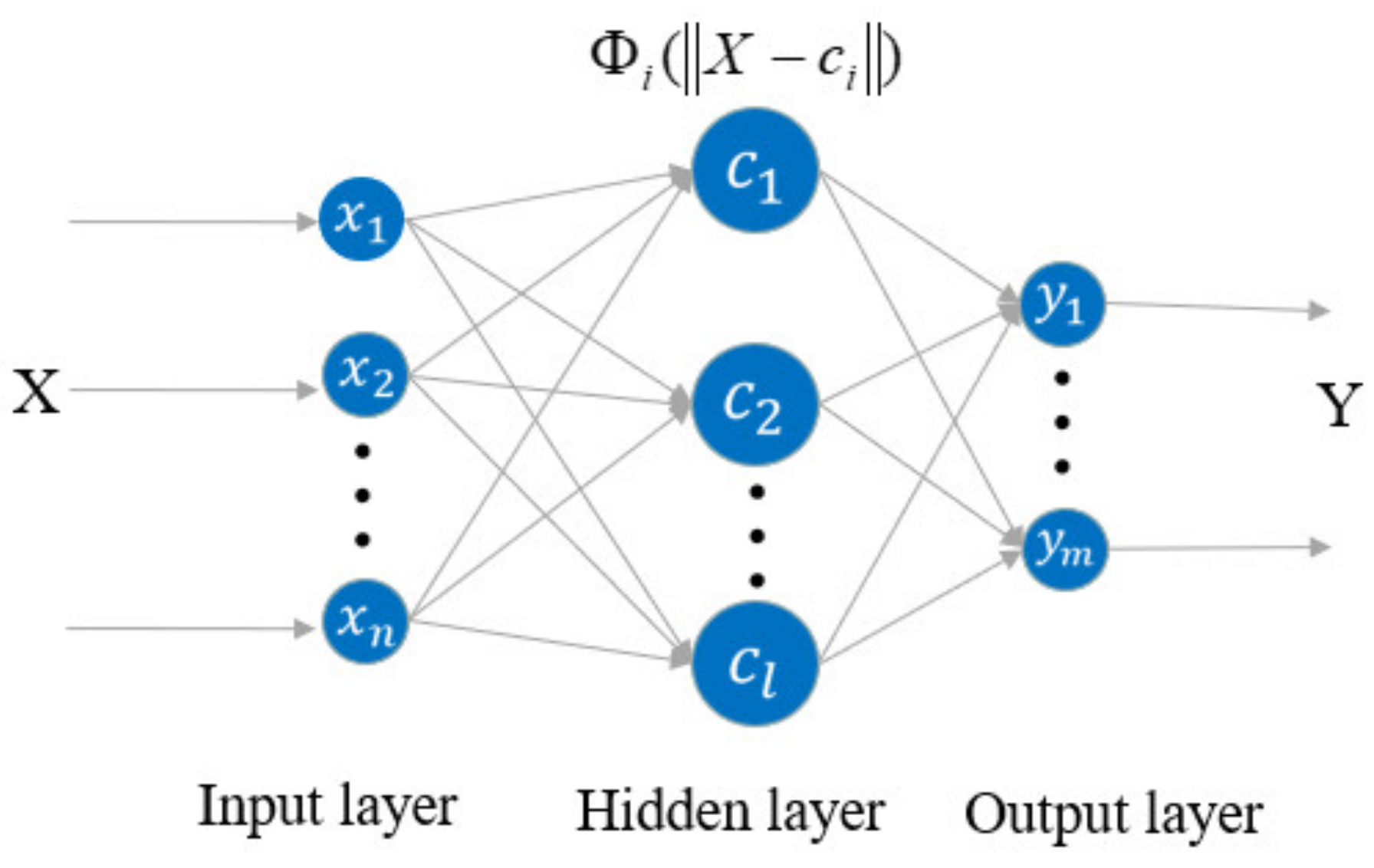
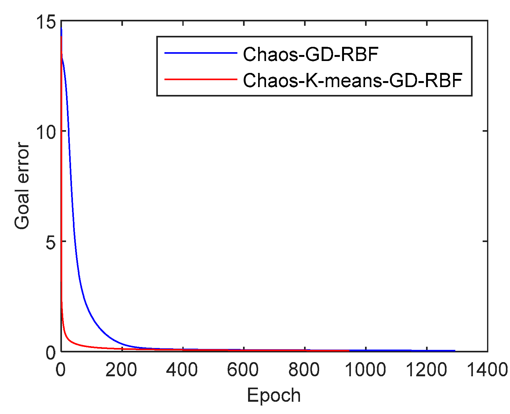
3.1. RBF Neural Network Modeling Based on K-Means Clustering Algorithm

Combined with the K-means clustering algorithm, the data centers of the $l$ hidden nodes are firstly determined by the unsupervised learning method in the RBF neural network. The expansion constant of the hidden nodes are confirmed according to the distance between the data centers. Then, the output weight vector W is calculated with the least square method (LSM) directly. The specific process of neural network training is described briefly as follows:

Set the sample input as $X_1,X_2,\cdots ,X_N$, and the corresponding sample output as $Y_1,Y_2,\cdots ,Y_N$. The cluster center at the k-th iteration is $c_1(k),c_2(k),\cdots ,c_l(k)$, and the corresponding cluster domain is $w_1(k),w_2(k),\cdots ,w_l(k)$.

(1) Select different initial cluster centers with number $l$, and set k to be 1. The initial sample selection can be random. However, different values must be selected for these initial data centers;

(2) Calculate the distance $‖X_j-c_i(k)‖,i=1,2,\cdots ,l,j=1,2,\cdots N$ between the sample input and the cluster center;

(3) Classify the sample input $X_j,X_j\in w_i(k)$ according to the minimum distance principle. This means that the input $X_j$ is classified as the i-th category as $i(X_j)=\underset{i}{\min }‖X_j-c_i(k)‖,i=1,2,\cdots ,l$;

(4) Recalculate the new cluster centers:

$$c_i(k+1)=\frac{1}{N_i}{\displaystyle \sum _{x\in w_i(k)}x, }i=1,2,\cdots ,l,$$

(8)

where $N_i$ is the number of samples contained in the i-th clustering domain $w_i(k)$;

(5) If $c_i(k+1)\ne c_i(k)$, go to step (2) to repeat the above process. If $c_i(k+1)=c_i(k)$, turn to step (6) with the ending of clustering;

(6) Determine the expansion constant of hidden nodes according to the distance between each cluster center. The expansion constant of the hidden node is taken as ${\delta }_i=\kappa d_i$, where $\kappa$ is the overlap coefficient. The selection of $d_i$ is valued as $d_i=\underset{i}{\min }‖c_j-c_i(k)‖$, which is the minimum distance between the i-th data center and the other data center;

(7) According to the determined data center and expansion constant of the hidden node, the least square method is used to directly calculate the output weight matrix W.

3.2. RBF Neural Network Modeling Based on Gradient Descent Algorithm

The first step of the procedure is to initialize the data center and fix the expansion constant and output weight in the RBF neural network modeling based on the gradient descent method. The method is applied in an optimization strategy, minimizing the objective function to realize the adjustment of hidden nodes, the expansion constant, and output weight. The objective function of a single-output RBF neural network learning with forgetting factor is set as:

$$E=\frac{1}{2}{\displaystyle \sum _{j=1}^N{\beta }_j{e}_j^2},$$

(9)

where ${\beta }_j$ is the forgetting factor, and the error signal $e_j$ is defined as:

$$e_j=y_j-F(X_j)=y_j-{\displaystyle \sum _{i=1}^l{w}_i{\mathrm{\Phi }}_i(X_j)}.$$

(10)

The gradient of the neural network function F(X) to the data center $c_i$, the expansion constant ${\delta }_i$ and the output weight $w_i$ can be expressed, respectively, as:

$${\nabla }_{c_i}F(X)=\frac{2w_i}{{\delta }_i^2}{\mathrm{\Phi }}_i(X)(X-c_i),$$

(11)

$${\nabla }_{{\delta }_i}F(X)=\frac{2w_i}{{\delta }_i^3}{\mathrm{\Phi }}_i(X){‖X-c_i‖}^2,$$

(12)

$${\nabla }_{w_i}F(X)={\mathrm{\Phi }}_i(X).$$

(13)

Considering the influence of the training samples and the forgetting factor, the adjustment amount of the data center $c_i$, the expansion constant ${\delta }_i$ and the output weight $w_i$ is set in the following definitions as:

$$\mathrm{\Delta }{c}_i=\eta \frac{w_i}{{\delta }_j^2}{\displaystyle \sum _{j=1}^N{\beta }_i{e}_i}{\mathrm{\Phi }}_i(X_j)(X_j-c_i),$$

(14)

$$\mathrm{\Delta }{\delta }_i=\eta \frac{w_i}{{\delta }_j^3}{\displaystyle \sum _{j=1}^N{\beta }_j{e}_j}{\mathrm{\Phi }}_i(X_j){‖X_j-c_i‖}^2,$$

(15)

$$\mathrm{\Delta }{w}_i=\eta {\displaystyle \sum _{j=1}^N{\beta }_j{e}_j}{\mathrm{\Phi }}_i(X_j),$$

(16)

where ${\mathrm{\Phi }}_i(X_j)$ is the output of the i-th hidden node to $X_j$, and $\eta$ is the learning rate.

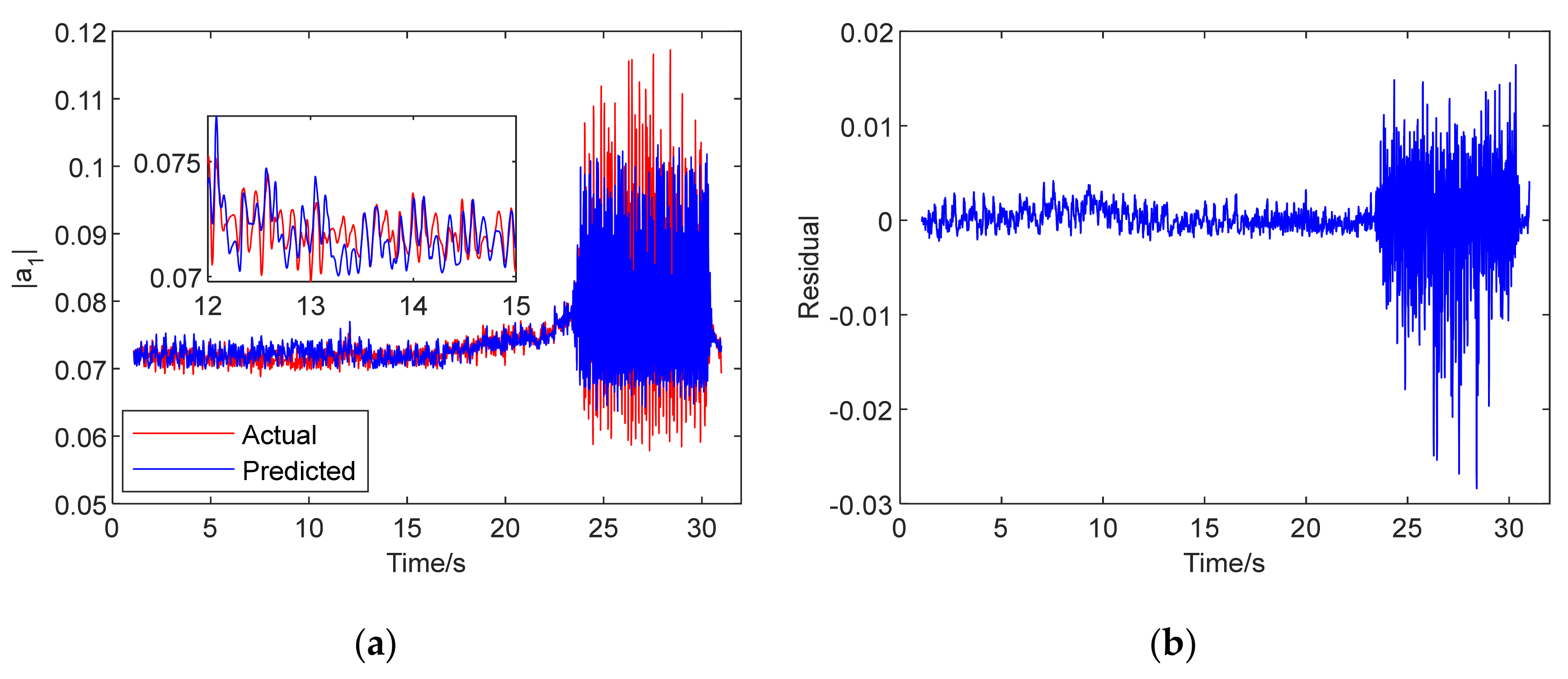
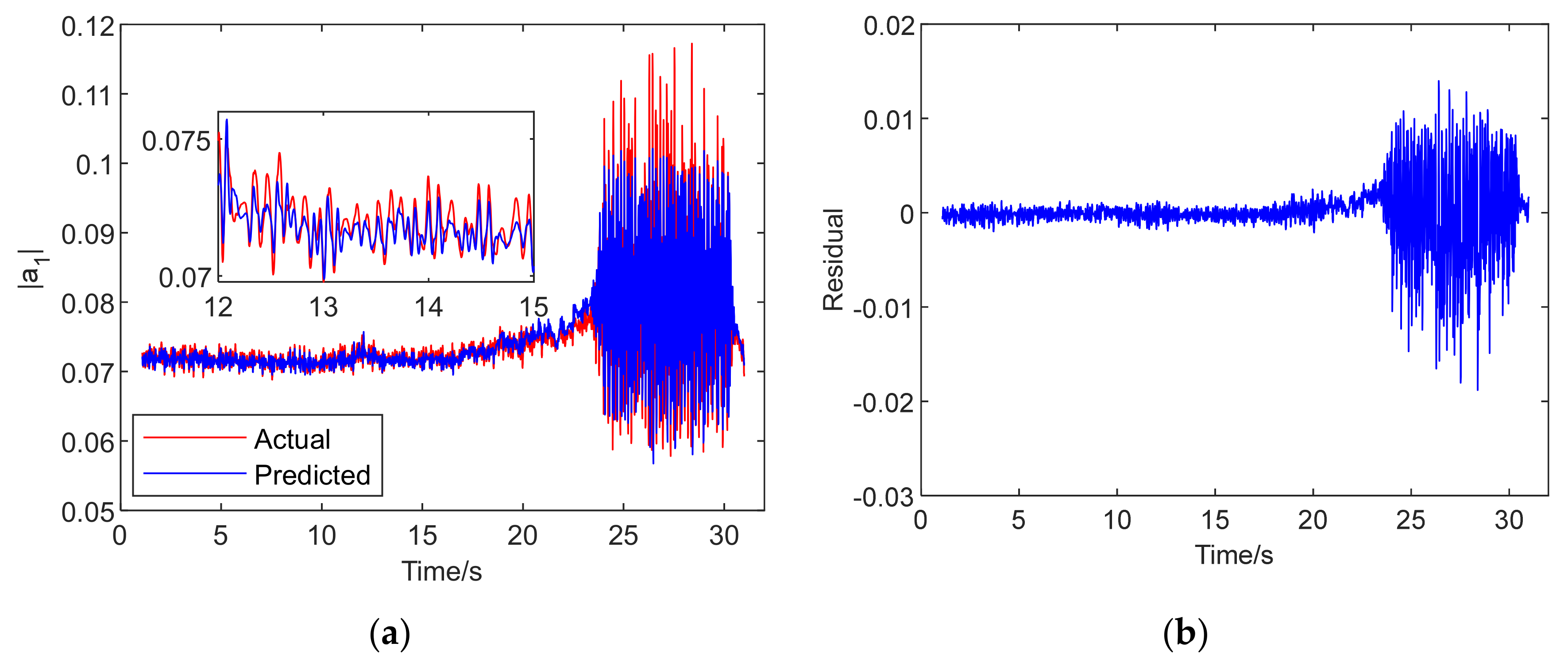
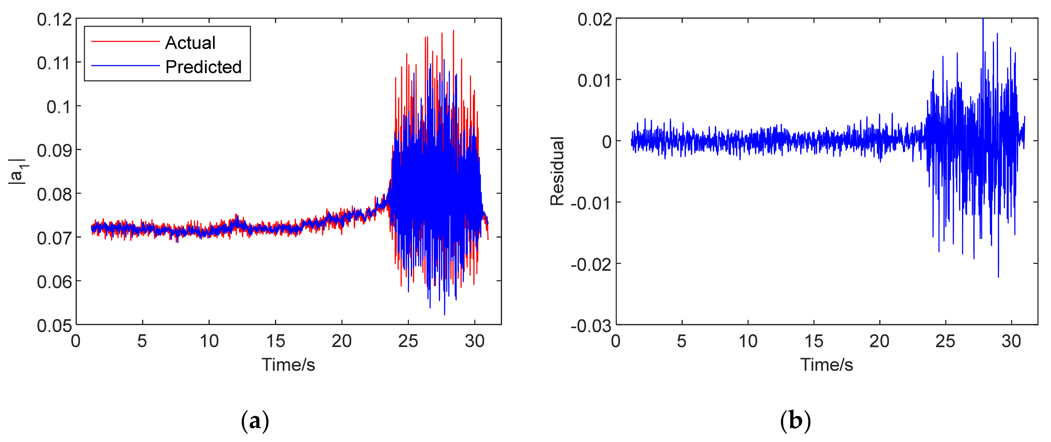
3.3. Dynamic System Modeling with the Hybrid Neural Network

Based on the pressure data of circumferential measuring points in the compressor, the spatial mode takes the form to reveal the essential characteristics of the rotating stall in the system. In this section, on the basis of phase space reconstruction of the spatial modal amplitude sequence |a1|, the nonlinear property of the dynamic system is modeled by the neural network with its chaotic character.

The reconstruction of the phase space of the modal amplitude |a1| with time series is needed firstly to discover the “deterministic” law of the singular attractor in the chaos. It is pointed out that in reference [20], the selection of delay time $\tau$ did not require a specific restriction for the noiseless chaotic sequence according to Takens’ theorem. It was also found that even if the delay time $\tau$ was not taken, an optimal value for reconstructing the phase space, it would only affect the Euclidean geometry of the reconstructed attractor, and then affect the calculation on the correlation dimension. The nonlinear properties of the dynamic can still be unambiguously reflected by the reconstructed attractor [21]. Meanwhile, if the delay time $\tau$ is taken as a larger value, this means that the nonlinear relationship to be fitted by the prediction model will be more complex. The cost of computation is increased with adding another layer of difficulty. Therefore, the key parameter $\tau$ of phase space reconstruction should be a relatively small value according to the complexity of the system. However, this kind of parameter selection needs to be implemented after an effective noise filtering of the observation sequence. After the solution of signal noise reduction, the delay time $\tau$ was chosen to be 1 for reconstructing the phase space in the modeling algorithm of this paper. Under this condition, the result indicated that the chaotic attractor was fully opened, with the requirement of dimension m greater than 3. Therefore, according to Figure 6b, the optimal selection of embedding dimension m was equal to 20 in the phase space reconstruction in this paper.

By using the interval sampling method, the whole dataset of amplitude sequence |a1| is divided into two sets of data for the spatial mode. One is the training set, and the other is the prediction set. After determining the training set and the prediction set, the process of reconstruction in the phase space is performed. On the basis of phase space reconstruction, a fusion neural network modeling solution was proposed for the prediction of instability in the system, which was combined with the K-means algorithm and the GD algorithm. In the chaotic phase space, the K-means algorithm was adopted to cluster the sample input to determine the data center and expansion constant of the hidden nodes in the RBF network. After the computation procedure, we assigned the obtained data center and extension constant to the GD algorithm as its initial value. Then, the output weight of the GD algorithm was initialized. Finally, the adjustment of the data center, expansion constant, and output weight of each hidden node was realized by the optimization strategy while minimizing the objective function. Thus, the Chaos–K-means–GD–RBF hybrid neural network model was established with the above procedure. Based on the characteristics of chaos, this model can fully display the laws of the system in a high-dimensional space. The embedding dimension m of the system is taken as the number of input layers, and the point vector data in the phase space is selected as the input data in the model. It not only meets the input requirement of the system, but also contains the complete regular pattern of the system.

Assume the network input as $X_i=a(i),a(i+1),\cdots ,a(i+m-1)$, the network output as $Z_i=a(i+m+S-1)$, $i=1,2,\cdots ,N-(m-1)\tau$, where $a$ represents the training set or prediction set |a1|, S is the number of prediction steps, N is the total number of data points in the training set or prediction set, m is the embedding dimension, and $\tau$ is the delay time. In this current research, the number of hidden layers in the neural network was set to be 12 with the maximum times of training 5000. The accuracy of the prediction model was evaluated by the performance of the neural network with mean absolute error (MAE) and root mean square error (RMSE). The prediction error was reflected by MAE, and the deviation between the values of the prediction and the experiment was measured by RMSE. The definition is described as follows:

$$MAE=\frac{{\displaystyle {\sum }_{i=1}^N\left|Y_{pi}-Y_{ai}\right|}}{N},$$

(17)

$$RMSE=\sqrt{\frac{{\displaystyle {\sum }_{i=1}^N{(Y_{pi}-Y_{ai})}^2}}{N}},$$

(18)

where N is the number of observational data, Y_pi represents the predicted value for the prediction set, and Y_ai represents the true value in the prediction set.

The results of the single-step prediction modeling for the spatial mode of the system are indicated in Figure 8, Figure 9 and Figure 10, which were established by the Chaos–K-means–RBF model, Chaos–GD–RBF model and the Chaos–K-means–GD–RBF fusion model, respectively, under the same parameters. The detailed windows in the figures show the zoomed results in the period of 12 s–15 s. It can be seen directly that the effect of the prediction approximation was the best for the Chaos–K-means–GD–RBF hybrid neural network model. On the contrary, a relatively poor approximation is visible for Chaos–K-means–RBF neural network model. Similarly, with the comparison on the preliminary results of residuals in Figure 8, Figure 9 and Figure 10, the residual errors of the Chaos–K-means–GD–RBF fusion model were significantly smaller than the other two neural network models.

In order to assess the performances of prediction quantitatively for the neural network models mentioned above, the MAE and RMSE were calculated as the indicators for evaluation in this paper. The computation results are revealed in

Table 2. Performance comparison of neural network models.

Model	MAE	RMSE	MAE-1	MAE-2
Chaos–K-means–RBF	1.8 × 10−3	3.3 × 10−3	8.38 × 10−4	4.5 × 10−3
Chaos–GD–RBF	1.5 × 10−3	2.6 × 10−3	6.46 × 10−4	3.8 × 10−3
Chaos–K-means–GD–RBF	1.2 × 10−3	2.6 × 10−3	2.67 × 10−4	3.6 × 10−3

. The numerical values of MAE and RMSE represent the average absolute error and root mean square error of the entire data. Moreover, the average absolute errors of the dataset before and after the time of 23 s are expressed by MAE-1 and MAE-2, respectively. Through the comparison of errors listed in Table 2, it is indicated that the Chaos–K-means–GD–RBF hybrid neural network model proposed in this research reflected a better modeling ability with an accurate prediction.

The contrast of variation on error reduction is pictured in Figure 11 between the Chaos–GD–RBF neural network model and the Chaos–K-means–GD–RBF hybrid neural network model during the training process. It can be seen that the reduction of error decreased more quickly in the Chaos–K-means–GD–RBF fusion model. Simultaneously, the cost of calculation was compared quantitatively. By extracting the average time of five steps in computation process, the time cost for determining three parameters in the Chaos–GD–RBF model was 32.8 s, and that of the Chaos–K-means–GD–RBF model was 20.43 s. In terms of calculation cost, an obvious advantage can be seen in the processing efficiency of the Chaos–K-means–GD–RBF model. From the analysis above, it can be concluded that the hybrid neural network model proposed in this paper exhibited excellent performances on the modeling of a nonlinear dynamic system with an accurate prediction. In a combination with the K-means algorithm and the GD algorithm, the calculation accuracy was improved in the hybrid neural network model based on phase space reconstruction. The computational efficiency was also promoted significantly, as compared with the two methods mentioned above.

4. Instability Prediction of Dynamic System with Identification Strategy

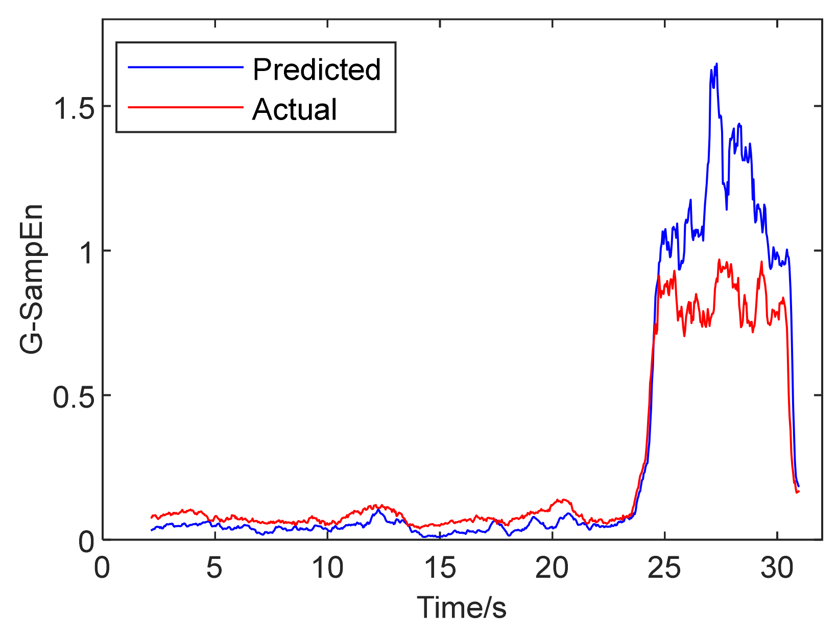
4.1. Single-Step Prediction Model Based on Sample Entropy Recognition Strategy

In this section, the Global Sample Entropy algorithm (G-SampEn) is performed to dynamically analyze the results of the single-step prediction model established by the Chaos–K-means–GD–RBF neural network in Figure 10. Based on the principle of sample entropy algorithm, the analysis of entropy can describe the variation of nonlinearity in the system at adjacent times. Thus, the precursor of instability for the system can be identified for the stall inception. Considering the sample data frequency and the calculation cost, the number of data points was selected as 250 for the sliding window W, and the interval of the dataset was taken for 10 in the sliding step h. In the G-SampEn algorithm, the parameters of embedding dimension m and similarity tolerance r were valued as 2 and 0.2 Std, respectively, in which Std represents the standard deviation of the whole window data.

Figure 12 shows the curves of dynamic G-SampEn for the predicted model and the actual value of the first-order spatial mode amplitude. It can be seen from the figure that the tendency of variation was almost the same both for the prediction and actual value in the analysis of G-SampEn. As the system approached the boundary of instability, the magnitudes of sample entropy showed an obvious mutation with a rapid increase. With the occurrence of the rotating stall, the entropy of system was significantly greater than that under normal operating conditions. From the above analysis, it can be concluded that the developing process of the dynamic system showed obvious mutation phenomena at the unstable boundary, based on the G-SampEn analysis of the spatial mode. The developing trend of the prediction was consistent with the property of real data.

In order to accurately identify the stall precursor, an identification strategy with difference quotient criterion is introduced this paper based on the dynamic G-SampEn of prediction. According to the amplitudes A(k) of dynamic G-SampEn, the difference quotient is calculated by $f_a=\left|A(k+1)-A(k)\right|/\mathrm{\Delta }h$, where $\mathrm{\Delta }h$ represents the sliding step time, and $f_a$ reflects the dynamic rate on the variation of G-SampEn value with respect to the time. As shown in Figure 13, the disturbance of the difference quotient emerged obviously when the rotating stall was about to happen. Moreover, the rapid increase in the difference quotient can be regarded as a significant feature of the system approaching instability. The moment with the rapid increase in the difference quotient value corresponded to the moment of the dynamic G-SampEn happening with a mutation. This exact time was judged as an identification signal for the pre-stall time with the difference quotient reaching the first peak, exceeding the threshold, as pointed out by A in Figure 13. The pre-stall time of recognition was marked as 23.718 s, which was ahead of stall time 23.97 s. In addition, the time interval of each step in the single-step prediction model was 4 ms. Therefore, an early warning of the stall inception can be given at about 256 ms (10.7 revolutions) in advance, based on the Chaos–K-means–GD–RBF neural network single-step model with an identification strategy of the sample entropy algorithm.

4.2. Multi-Step Prediction Model Based on Sample Entropy Recognition Strategy

In the case of a fixed sampling frequency, the time predicted for the stall inception mainly depends on the number of prediction steps ahead. Taking into account the time cost in calculation, the forecasting with single-step prediction model may not be able to meet the actual demand. For the sake of achieving a larger time margin for the rotating stall control, a multi-step prediction model with a neural network is explored in this section for the inception recognition. Compared with the single-step prediction, the feature of inception can be recognized to an earlier date, which reflects a superiority of prediction in multiple steps. The input of the neural network model of multi-step prediction is the same as that of single-step prediction model. However, a distinction in output exists between the two models. In the Section 3.3, the network output is defined as $Z_i=a(i+m+S-1)$, $i=1,2,\cdots ,N-(m-1)\tau$. In this definition, the parameter S as the number of prediction steps is valued with an integer larger than 1.

In theory, an early warning of stall inception can be shifted forward with more prediction steps. However, in fact, as the number of multiple steps for prediction increases, the accuracy of this neural network model declines to a certain extent. Since the phase difference between the real value and the prediction will be enlarged by the multi-step model, the network performance is measured by the combination of phase difference, MAE, and RMSE in this section. For two discrete sampled continuous signals X(n) and Y(n) with phases $(\omega t+{\phi }_1)$ and $(\omega t+{\phi }_2)$, respectively, the phase difference $\mathrm{\Delta }\phi$ is calculated with the cross-correlation algorithm [22]. The formula is stated as:

$$\mathrm{\Delta }\phi =\omega t+{\phi }_2-(\omega t+{\phi }_1)=\arccos (\frac{R_{xy}(0)}{\sqrt{R_x(0)R_y(0)}}),$$

(19)

$$R_x(0)=\frac{1}{N}{\displaystyle \sum _{n=0}^{N-1}{X}^2(n)},$$

(20)

$$R_y(0)=\frac{1}{N}{\displaystyle \sum _{n=0}^{N-1}{Y}^2(n)},$$

(21)

$$R_{xy}(0)=\frac{1}{N}{\displaystyle \sum _{n=0}^{N-1}X(n)Y(n)}.$$

(22)

With the increasing steps of multi-step prediction, the residuals of MAE, RMSE, and phase difference in the model gradually become larger. In the developing process, the modeling for system instability may not be able to provide an effective identification on inception, when the errors exceed a certain value. Through the comparison of results, the threshold of phase difference for multi-step prediction was set as 2D₀, of which D₀ (0.74°) was the phase difference of the single-step prediction model. Within the limitation of the phase difference threshold, the maximum number of prediction steps was identified for the optimal choice with relatively small errors. After the computation within the error range, the best performance of the prediction model in multi-step was found at the selection of the parameter S as 18. This means that the hybrid neural network model established can predict the amplitude of spatial mode 18 steps in advance, within the error range.

The results of the multi-step prediction are shown in Figure 14, indicating the prediction of the first-order spatial modal amplitude and the residual in the process. Due to the increase in the steps in the multi-step prediction, the residual was enlarged in modeling the system compared with the one-step prediction. The dynamic G-SampEn of spatial mode amplitude in multi-step prediction is shown in Figure 15, with a comparison to the actual value of the experiment. The parameter setting of the G-SampEn algorithm was the same as that of the single-step prediction in Section 4.1. In spite of the differences in numerical values, the tendency of variation was still consistent with the experiment data for the same mutation time. The principle of difference quotient was also introduced into the analysis on the dynamic G-SampEn of multi-step prediction to effectively identify the pre-stall moment. The computation result is revealed in Figure 16. The moment with a rapid increase in the difference quotient was regarded as the instability boundary of the system for the stall. The first peak of mutation, pointed to by mark A in the difference quotient, is considered to be the identification signal. This moment was recognized as 23.746 s. In the meantime, the time interval of 18 steps in the multi-step prediction model was 72 ms. Therefore, based on the Chaos–K-means–GD–RBF hybrid neural network multi-step model, the inception of the system stability can be distinguished about 296 ms (12.3 revolutions) ahead, with the identification strategy of the sample entropy algorithm.

5. Discussion on Application

From the perspective of analysis on the modal wave, it was found that the indication of stall inception could be caught with the feature extracted by the circumferential spatial mode. The significant mutation in the sample entropy based on the spatial modal amplitude can be considered as a pronounced mark, well before the imminence of a stall. This moment is supposed to be the position of identification on stall inception. Therefore, the pressure data of each measuring point was fused into the spatial mode to express the essence of the stall phenomenon. This kind of method of data processing effectively avoids the problems of inaccurate identification of a single measuring point only depending on pressure.

On this basis of reconstructing the spatial modal amplitude, neural network modeling was conducted to establish a prediction model of the dynamic system for the rotating stall. The procedure of modeling was carried out with single-step and multi-step prediction. The difference between the single-step method and the multi-step method lies in the network output, resulting in different time intervals for forecasting. In the current research, the outputs of the neural network model were set as $Z_i=a(i+m)$ for the single-step prediction, and $Z_i=a(i+m+17)$ for multi-step prediction with 18 steps. From the results revealed, a better prediction accuracy was found for the single-step prediction model compared with the model with multi-steps. However, in fact, multi-step prediction was much more practical in the process of forecasting, such as for the quantity of identification time in advance. In the computation of model prediction, the calculation time was cost with 8.6 ms for each time step under single core computing with the Intel core i5-4570 CPU. This calculation cost was significantly less than the time interval 72 ms of the multi-step forecasting. So, it was enough to predict the system state in next time step by deducting the cost. With a total warning time of 296 ms ahead, the application of dynamic system modeling for stall inception still needs further research with examination. In future research, the algorithm with system modeling needs to be further improved in the accuracy of multi-step prediction, so as to strive for a greater margin for rotating stall identification. The technology of deep neural network modeling is worthy of further exploration.

6. Conclusions

Focusing on the identification of the stall inception in an axial compressor, a hybrid neural network model was proposed in this research for modeling the stability of a dynamic system. Based on the data fusion of the amplitude of the spatial mode, a hybrid neural network was adopted to represent the properties of the system by artificial intelligence learning. After the process of phase space reconstruction of the chaotic sequence, the Chaos–K-means–GD–RBF fusion model was established with a combination of K-means and GD methods. By taking the strategy of global sample entropy and difference quotient criterion identification, a warning of inception can be suggested in advance of the stall arrival. The main conclusions are summarized as follows:

(1) With the analysis of the spatial mode, a traveling wave was shown in the development of the amplitude with the first-order spatial mode. This method of data processing can effectively avoid the inaccurate recognition of single or multiple measuring sensors only depending on pressure. The variation of spatial modal amplitude accurately reflects the basic feature of a dynamic system in a compressor from normal operating conditions to the stall condition. With proof of the positive Lyapunov exponent in the system, it is indicated that the chaos series was proven during the instability of the dynamic system in the development of the rotating stall;

(2) On basis of phase space reconstruction of the spatial modal amplitude sequence, the nonlinear property of the dynamic system was modeled by the neural network with its chaotic character. In combination with the K-means algorithm and the GD algorithm, the Chaos–K-means–GD–RBF hybrid neural network model was proposed in this paper for rotating stall prediction. As seen from the computation results, it can be concluded that the established hybrid neural network model exhibited excellent performances on the modeling of nonlinear dynamic systems, with an accurate prediction. The computational efficiency was also significantly promoted, compared with the two methods mentioned;

(3) Based on the principle of the sample entropy algorithm, the precursor of instability can be identified by the variation of nonlinearity in the system at adjacent times for the stall inception. As the system approaches the boundary of instability, the magnitudes of sample entropy show an obvious mutation with a rapid increase. An identification strategy with difference quotient criterion was introduced, based on the dynamic G-SampEn of prediction. Thus, the rapid increase in the difference quotient was regarded as a significant feature of the system approaching instability. Therefore, by taking the strategy of global sample entropy and difference quotient criterion identification, a warning of inception can be suggested in advance of 12.3 revolutions (296 ms) with the Chaos–K-means–GD–RBF hybrid neural network multi-step model, before the stall arrival.

References

1. Epstein, A.H.; Williams, J.E.F.; Greitzer, E.M. Active suppression of aerodynamic instabilities in turbomachines. J. Propuls. Power 1989, 5, 204–211. [Google Scholar] [CrossRef]
2. Mcdougall, N.M.; Cumpsty, N.A.; Hynes, T.P. Stall inception in axial compressors. J. Turbomach. 1990, 112, 116–125. [Google Scholar] [CrossRef]
3. Day, I.J.; Breuer, T.; Escuret, J.; Cherrett, M.; Wilson, A. Stall inception and the prospects for active control in four high-speed compressors. J. Turbomach. 1999, 121, 18–27. [Google Scholar] [CrossRef]
4. Paduano, J.D. Analysis of compression system dynamics. Act. Control Engine Dyn. 2002, 8, 1–36. [Google Scholar]
5. Tahara, N.; Kurosaki, M.; Ohta, Y.; Ohta, E.; Nakajima, T.; Nakakita, T. Early stall warning technique for axial-flow compressors. J. Turbomach. 2007, 129, 448–456. [Google Scholar] [CrossRef]
6. Liu, B.; Lei, Y. Design and implementation of aerodynamic instability embedded early warning system for compressor. Meas. Control Technol. 2010, 29, 68–71. [Google Scholar]
7. Cameron, J.D.; Morris, S.C. Analysis of axial compressor stall inception using unsteady casing pressure measurements. J. Turbomach. 2013, 135, 021036. [Google Scholar] [CrossRef]
8. Liu, Y.; Li, J.; Du, J. Application of fast wavelet analysis on early stall warning in axial compressors. J. Therm. Sci. 2019, 28, 837–884. [Google Scholar] [CrossRef]
9. Xu, X.; Wang, S.; Liu, J.; Liu, X. Intelligent prediction of fan rotation stall in power plants based on pressure sensor data measured In-Situ. Sensors 2014, 14, 8794–8809. [Google Scholar] [CrossRef] [PubMed] [Green Version]
10. Wang, C.; Wen, B.H.; Si, W.J.; Peng, T.; Yuan, C.Z.; Chen, T.R.; Lin, W.Y.; Wang, Y.; Hou, A.P. Modeling and detection of rotating stall in axial flow compressors: Part I: Investigation on high-order M-G models via deterministic learning. Acta Autom. Sin. 2014, 40, 1265–1277. [Google Scholar]
11. Wang, C.; Si, W.J.; Wen, B.H.; Zhang, M.M.; Wang, Y.; Hou, A.P. Modeling and detection of rotating stall in axial flow compressors: Part II: Experimental study for a low-speed compressor in Beihang University. Control Theory Appl. 2014, 31, 1414–1422. [Google Scholar]
12. Hipple, S.M.; Bonilla-Alvarado, H.; Pezzini, P.; Shadle, L.; Bryden, K.M. Using machine learning tools to predict compressor stall. J. Energy Resour. Technol. 2020, 142, 070915. [Google Scholar] [CrossRef]
13. Zhang, M.M.; Hou, A.P. Investigation on stall inception of axial compressor under inlet rotating distortion. J. Mech. Eng. Sci. 2017, 231, 1859–1870. [Google Scholar] [CrossRef]
14. Zhang, M.M.; Li, K.Y.; Dong, W.J. Identification on rotating stall precursor of a low-pressure compressor via periodic perturbations. Propuls. Technol. 2016, 37, 871–878. [Google Scholar]
15. Takens, F. Detecting Strange Attractors in Turbulence. Dynamical Systems and Turbulence. Warwick 1980; Springer: Berlin/Heidelberg, Germany, 1981; pp. 366–381. [Google Scholar]
16. Wallot, S.; Mønster, D. Calculation of average mutual information (ami) and false-nearest neighbors (fnn) for the estimation of embedding parameters of multidimensional time series in matlab. Front. Psychol. 2018, 9, 1679. [Google Scholar] [CrossRef] [Green Version]
17. Yang, J.H.; Cai, H.R.; Zou, Z.J.; Xu, W.D.; Wu, J. Chaos analysis and decoupling adaptive backstepping control of doubly fed wind power system. Acta Energ. Sol. Sin. 2019, 40, 3605–3612. [Google Scholar]
18. Moradi, M.J.; Roshani, M.M.; Shabani, A. Prediction of the load-bearing behavior of SPSW with rectangular opening by RBF network. Appl. Sci. 2020, 10, 1185. [Google Scholar] [CrossRef] [Green Version]
19. Cheng, J.; Qi, B.; Chen, D. Modification of an RBF ANN-based temperature compensation model of interferometric fiber optical gyroscopes. Sensors 2015, 15, 11189–11207. [Google Scholar] [CrossRef] [PubMed] [Green Version]
20. Han, M. Theory and Method of Chaotic Time Series Prediction; China Water Power Press: Beijing, China, 2007. [Google Scholar]
21. Wolf, A.; Swift, J.B.; Swinney, H.L. Determining Lyapunov exponents from a time series. Phys. D Nonlinear Phenom. 1985, 16, 285–317. [Google Scholar] [CrossRef] [Green Version]
22. Zheng, S.F.; Chen, S.M.; Di, J.H.; Wang, B.Y. Phase difference measurement of sinusoidal signal based on multi-layer cross-correlation. J. Astronaut. Metrol. Meas. 2012, 32, 34–40. [Google Scholar]
Figure 1. Schematic diagram of the compressor experiment. (a) Compressor test rig; (b) sensors’ location.
Machines 10 00122 g001
Figure 2. Original output voltage signal diagram at measuring point #1.
Machines 10 00122 g002
Figure 3. Pressure signals after resampling and denoising.
Machines 10 00122 g003
Figure 4. The first-order spatial mode amplitude |a1|in development process.
Machines 10 00122 g004
Figure 5. Frequency diagram of spatial mode.
Machines 10 00122 g005
Figure 6. Computation results of the delay time τ and the embedding dimension m: (a) optimal delay time τ ; (b) optimal embedding dimension m.
Machines 10 00122 g006
Figure 7. RBF neural network structure.
Machines 10 00122 g007
Figure 8. Result of Chaos–K-means–RBF neural network model: (a) prediction; (b) residual.
Machines 10 00122 g008
Figure 9. Result of Chaos–GD–RBF neural network model: (a) prediction; (b) residual.
Machines 10 00122 g009
Figure 10. Result of Chaos–K-means–GD–RBF neural network model: (a) prediction; (b) residual.
Machines 10 00122 g010
Figure 11. Comparison of the error reduction during the training process.
Machines 10 00122 g011
Figure 12. Dynamic G-SampEn of the first-order spatial mode amplitude.
Machines 10 00122 g012
Figure 13. Difference quotient of the dynamic G-SampEn.
Machines 10 00122 g013
Figure 14. Multi-step prediction results: (a) prediction; (b) residual.
Machines 10 00122 g014
Figure 15. Dynamic G-SampEn of spatial mode amplitude in multi-step prediction.
Machines 10 00122 g015
Figure 16. Difference quotient of the dynamic G-SampEn in multi-step prediction.
Machines 10 00122 g016