Research on Guide Line Identification and Lateral Motion Control of AGV in Complex Environments

Abstract

During actual operations, Automatic Guided Vehicles (AGV) will inevitably encounter the phenomena of overexposure or shadowy areas, and unclear or even damaged guide wires, which interfere with the identification of guide wires. Therefore, this paper aims to solve the shortcomings of existing technology at the software level. Firstly, a Fast Guide Filter (FGF) is adopted with the two-dimensional gamma function with variable parameters, and an image preprocessing algorithm in a complex illumination environment is designed to get rid of the interference of illumination. Secondly, an ant colony edge detection algorithm is proposed, and the guide wire is accurately extracted by secondary screening combined with the guide wire characteristics; A variable universe Fuzzy Sliding Mode Control (FSMC) algorithm is designed as a lateral motion control method to realize the accurate tracking of AGV. Finally, the experimental platform is used to comprehensively verify the series of algorithms designed in this paper. The experimental results show that the maximum deviation can be limited to 1.2 mm, and the variance of the deviation is less than 0.2688 mm².

1. Introduction

In recent years, with the development of vision-guided Automatic Guided Vehicle (AGV) systems, fast and accurate guide wire detection has attracted extensive research attention [1,2]. Lead detection is usually realized by images captured by a camera installed on the vehicle, and then the collected image is processed to extract meaningful information, such as the position, road mark, road boundary, and guidance direction. As the most basic traffic sign, a guide line boundary is the most important constraint restricting AGV driving. If the technology for recognition of the guide lines can be improved, the extraction of other information will be solved [3]. In addition, the identification and extraction of guide wires can not only provide motion guidance for AGV, but can also be applied to the active safety control system of other manned vehicles [4]. However, with the nonuniformity of pavement structures, damaged and stained guide wires, and changes in light, the detection of guide wires has become more and more difficult.

The identification technology of guide wires is mainly divided into three steps: image preprocessing, guide wire extraction, and navigation deviation calculation. Many scholars have carried out research on image processing under complex lighting conditions. Xing and other scholars proposed an illumination adaptive image segmentation method based on a relaxed constraint support vector machine (SVM) classifier and a kernel function to distinguish the original color features and illumination artifacts of road images. Different illumination regions were successfully partitioned and processed accordingly. However, this research method is highly dependent on color, and it is necessary to establish accurate and complete SVM classification learning samples in advance [5]. Wang designed an adaptive image enhancement algorithm based on Retinex theory, extracted the illumination component through the weighted sum of a multiscale Gaussian function, and finally used postprocessing for image enhancement. However, the edge preserving ability of Gaussian filter is very poor, so it cannot be used directly for lead extraction [6]. Huang proposed an adaptive image enhancement method based on chicken swarm optimization. The design objective function is the gray information entropy of the image, and the image enhancement problem is transformed into the problem of obtaining the optimal solution of the objective function [7]. This method is similar to many optimization algorithms. The continuous optimization and adjustment steps greatly reduce the real-time performance, so it is difficult to apply the algorithm to AGV. Liu and others extracted the illumination component through a multiscale Gaussian function, used the gamma function with fixed parameters to reasonably adjust the brightness value according to the uneven illumination area, and finally completed the adaptive brightness correction of the uneven illumination image. The algorithm has high real-time performance, but the edge preservation ability of Gaussian function filtering is very poor; for guide wire recognition, the preservation of edge details takes precedence over the preservation of color. Therefore, the effect of the simple use of a multiscale Gaussian function is not even as good as that of a low-scale Gaussian function alone [8]. At the same time, the parameters in the design of two-dimensional gamma function are solidified, which makes the image enhancement effect inconsistent under different lighting conditions. Scholars such as Shun proposed a physical illumination model. As long as the parameters in the model are correctly estimated, the low-illumination image can be directly restored by solving the model, but it depends on the accuracy of parameter estimation. At the same time, the algorithm has certain limitations for generating pseudocolor images in extremely dark areas [9]. Oh estimated the reflectivity through the brightness channel, used a nonlinear reflectivity reconstruction function to adaptively control the contrast, and reconstructed the brightness channel to reduce the number of halo artifacts in the processed image, but the applicability of the model needs to be further verified [10].

The control problem of path lateral tracking can be divided into two parts: the selection of preview points and lateral motion control. The driver preview model was first proposed by academician Guo. The driver’s awareness was expressed by establishing the driver’s preview model, and finally an in-loop controller considering the driver’s input was formed. Ding and other scholars established the driver model according to the optimal curvature under single-point preview. After selecting a preview point according to the vehicle speed, they obtained the optimal curvature to find the optimal path approaching the preview point [11]. Dong modified the steering wheel angle based on the traditional optimal preview driver model and designed an improved preview driver model [12]. Ren and other scholars established the vehicle lateral deviation dynamic and a yaw angle error model based on single-point preview [13]. Most studies, including the above studies, use the method based on vehicle speed and preview distance to calculate the preview point, but do not describe in detail how to find a reasonable preview point on the specified path—only using the preview point for subsequent motion control. At the same time, single-point preview has certain limitations. When the current attitude angle deviation of the vehicle is too large or the path curvature is too large, it is difficult to find a suitable preview point. At present, there is little research on multipoint preview. Zhao and others selected multiple preview points at equal intervals after selecting the first preview point; Xu and other scholars from the University of Michigan [14] proposed a path tracking algorithm based on optimal preview, introduced the multipoint preview road curvature in the finite time window into the augmented state vector, and reconstructed the nonlinear optimal control problem into an augmented LQR problem, but did not introduce the calculation of preview points in detail [15]. The lateral control scheme of path tracking includes a geometric model, a kinematic model, and a dynamic model. The geometric model relies on geometric models such as the relationship between vehicle attitude and position and Ackerman steering. The kinematic model further considers the motion equation of the vehicle, but does not involve the physical properties of the vehicle and the force on the vehicle. In short, the path tracking control method based on a geometric/kinematic model ignores the dynamic characteristics of the vehicle system and has a limited scope of application. Therefore, in order to obtain more accurate tracking control effect, the dynamic characteristics of the vehicle must be considered when designing the path tracking control, so as to control the accurate tracking of the vehicle under the condition of large curvature. At present, the algorithms applied based on a dynamic model mainly include PID control [16,17,18], fuzzy control [19,20,21], sliding mode control [22,23], and model predictive control [24,25,26]. Many authors have also applied PID and LQR to the control of Quadrotor, and the experimental results have shown that PID has good real-time performance but poor robustness, while LQR has better robustness and small steady-state error, but there is a delay problem [27,28]. Various algorithms have unique advantages; model predictive control, especially, has been widely used [29]. Although sliding mode control does not need to establish an accurate dynamic model and uses nonlinear theory to deal effectively with multidimensional complex coupling problems, the chatter phenomenon hinders its further application. Therefore, many scholars have carried out research on the disadvantages of buffeting, and many scholars use neural networks to adaptively approximate the uncertainty, so as to optimize it [30,31]. However, many deep learning algorithms, including neural networks, need a large number of accurate and reasonable training datasets, and the datasets have to be obtained by other algorithms. Chen and Zhang combined fuzzy control and sliding mode control, and adjusted the gain coefficient of switching term by using fuzzy rules, so as to achieve better control [32,33]. In addition to the improvement of the chatter phenomenon, we must focus on the analysis of its self-adaptability—that is, fuzzy control can change the parameters in SMC, which greatly improves the adaptability to different working conditions, and can achieve better control through the adjustment of parameters by fuzzy rules under different working conditions.

2. Establishment of Light Pretreatment Model

The main purpose of image preprocessing is to remove irrelevant information that interferes with the extraction of information of interest, restore the original information of the region of interest in the image, enhance the detectability of useful information, and improve the reliability of information matching, feature recognition, and region extraction. Generally, the main purpose of image preprocessing is to filter out all kinds of noise that may exist in the image to make the processed image smoother and clearer. However, the purpose of image preprocessing in this paper is to correct the image brightness, darken the area significantly higher than the average brightness, and brighten the area significantly lower than the average brightness, so as to get rid of the influence of light and make the final image brightness more uniform.

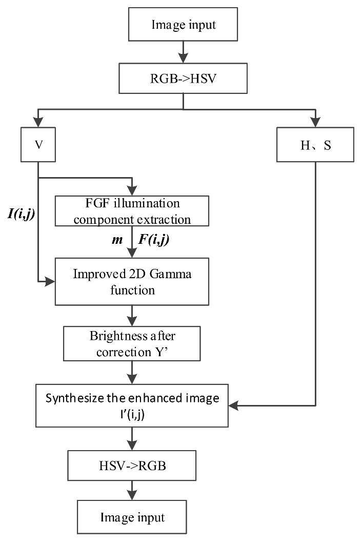
The image preprocessing process in a complex lighting environment is shown in Figure 1. When the system works, the camera with a frame rate of 30 fps continuously provides the image source as the system input. When the image processor receives the image, it first extracts the region of interest (ROI) according to the preview distance to avoid the processing of useless regions, so as to speed up the processing speed. In fact, the size of the ROI depends on factors such as camera angle and height. Generally speaking, the larger the ROI, the better. However, the larger the ROI, the lower the real-time performance. Therefore, the computing power of the processor should be considered to reasonably select the ROI. Then image preprocessing is carried out. Inspired by the Retinex algorithm, in order to solve the problem that uneven illumination in ROI area will interfere with the extraction, an image correction algorithm based on fast guided filtering and variable-scale two-dimensional gamma function is proposed. Due to only the HSV color space model meeting the requirements for brightness in this paper, there are parameters related to the transmittance or reflectance of the object, so it is necessary to transform the color space. Firstly, the RGB color space is converted to HSV color space, and the lightness component V is adjusted according to the illumination distribution. According to the distribution of illumination components, the overly bright or dark parts in the image are corrected by a variable-scale two-dimensional gamma function, so that the processed image is close to the image under uniform illumination. Finally, the adjusted v component is combined the with h and s components again, The processed image is obtained for subsequent lead extraction.

Inspired by the Retinex algorithm and introducing the guided filter with faster processing speed and stronger edge preservation to replace the traditional Retinex Gaussian filter, this paper designs an illumination component extraction algorithm based on a fast guided filter. I is the guide image and p is the input image. The input image p is processed to obtain the output image, so that the gradient of the output image is similar to the guide image, while the gray or brightness is similar to the input image. The algorithm mainly consists of the following steps:

(1)

Calculate the average value of each window of the guide image I and the filtered input image p and store it in meanofi and meanofp. In this paper, the guide image is the same as the filtered input image. At this time, the guide filtering is an edge preserving filtering operation, which can better ensure that the edge details remain in the original state while extracting the illumination component.

(2)

The variance of I and the covariance of I–P are calculated and stored in varofI and covofIp for the next least-squares optimization solution.

(3)

The least-squares method is optimized to solve a and b to minimize the reconstruction error between the output image and the original image. The regularization parameters used in this paper is ε = 0.05. If the variance is much less than ε, it is regarded as a flat region. On the contrary, the gradient is maintained in the region.

(4)

Calculate the mean value of each window in a and b and save it in meanofa and meanofb. The local window radius r used in this paper is 16 and the subsampling ratio is 4.

(5)

q = meanofa.∗I + meanofb, where q is the light component finally extracted.

In the above algorithm, there is a process of average value of each window in the image. Here, the box filtering method is used [34].

After the light component is extracted from the original image, it needs to be adjusted according to the brightness of the light at each pixel—that is, with different degrees of brightness correction according to the brightness of the light component in each region, so as to get rid of the influence of the light component. Gamma correction is a nonlinear global correction method. Nowadays, many scholars use a two-dimensional gamma function for image correction to effectively correct the uneven brightness of an image. On this basis, this paper makes some improvements and extensions, so that the adjustment force depends on the brightness of the illumination component, in order to improve the adaptability and rationality of the algorithm.

In general, gamma correction has the following standard forms:

$$O(i,j)=255{[\frac{I(i,j)}{255}]}^{\gamma },$$

(1)

where $I(i,j)$ is the input image (original v),$O(i,j)$ is the output image, and γ is the control parameter; the image darkens as a whole when $\gamma >1$, the image is lightened as a whole when $0<\gamma <1$, and the algorithm doesn’t make sense when $\gamma <0$. Scholars often use $2^{(F(i,j)-128)/128}$ to calculate γ. The gray value of white is 255 and the gray value of black is 0; the reason why the average value 128 is taken as the mean value of the illumination component and the base number 2 has not been clearly explained by scholars, but is often determined according to experience.

Based on the above research, this paper makes some adjustments to the traditional two-dimensional gamma function and establishes a relationship with the gray value distribution characteristics of the image to be processed, so that the image enhancement algorithm designed in this paper can have different adjustment intensity and strong environmental adaptability under different conditions. The value of γ is calculated as follows:

$$\gamma ’={\alpha }^{{}^{[(F(i,j)-m)/m]}},$$

(2)

where m is the luminance mean value of the illumination component f (i, j). Using m instead of the fixed value 128 can more reasonably represent the mean value of the current illumination component rather than the absolute mean value in the theoretical sense. Another change is the use of variable scales α. Instead of the fixed base 2, α the calculation is derived as follows.

Take the expected value of the improved gamma function formula, which should be equal to 128 in theory. The derivation is as follows:

$$\frac{\ln 0.5}{\ln (\frac{\overline{I}}{255})}={\alpha }^{{}^{[(F(i,j)-128)/128]}}.$$

(3)

Two limit cases are taken for analysis; the illumination component F(i, j) is all black or all white. At this time, two limit cases can be obtained for α values:

$$\left\{\begin{array}{l}{\alpha }_{white}\cong \frac{\ln (\frac{\overline{I}}{255})}{\ln 0.5}, \mathrm{when} F(i,j)=255\\ {\alpha }_{black}\cong \frac{\ln (0.5)}{\ln (\frac{\overline{I}}{255})}, \mathrm{when} F(i,j)=0\end{array}\right..$$

(4)

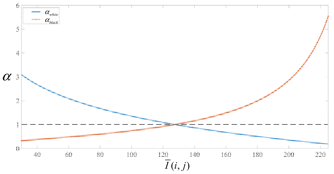
The two equations are represented by curves, as shown in Figure 2. Considering that the gray value of the actual image is not greater than 225 or less than 25, 25 and 225 are selected as the upper and lower limits of the interval of independent variables $\overline{I}$ (the algorithm cannot be applied to extremely bright and dark scenes beyond this range). When the average gray value of the original image $I$ is 128, the two curves coincide. In this paper, the curve above the dotted line is taken as α. When the mean value of illumination is less than 128, we use the α_white curve to calculate; otherwise, it is an α_black curve calculation. The advantage of this is that it can establish a relationship with the average gray value of the original image, so that the intensity of the image correction changes with the content of the original image. Images that are too bright or too dark will be adjusted significantly, while more balanced images will almost maintain the original state.

3. Extraction Method of Guide Wire against Line Interference

An ant colony algorithm is designed to extract the edge of guide wire. The pheromone released when the ant colony passes through the path is used as the judgment basis of edge points, screened through volatilization and aggregation mechanism, and the finally retained pheromone is extracted as the guide edge. The specific steps of the ant colony-like algorithm designed in this paper are as follows:

(1)

Initial position. The number of pixel rows is determined according to the resolution of the collected image, so that the number of ants is equal to the number of rows—that is, only one ant is placed in each row. The initial position of the ant is the leftmost or rightmost column of the image. This paper takes the leftmost column as an example.

(2)

Transfer. It is stipulated that each ant can only walk to the right. When passing the first point with a gray value of 255 (column I), record the number of columns I, leaving pheromone concentration η₁. If there is no pixel with a gray value of 255 in the subsequent I + X column, volatilize the pheromone in column I and continue to search right from column I + 1. If there are points with a gray value of 255 in the I + X column, record the following numbers and leave pheromones η₂; at the same time, set the pheromone concentration in column I to η₂ and continue to search to the right, with I + 1 as the starting column. When ants pass through pheromones η₂, continue to judge the gray value separated by X pixels until it exceeds the range of the image matrix. X is related to the width of the guide wire, which is the number of pixels occupied by the guide wire in each row of the collected image. The possible small distortion or “far small near large” of the guide wire in the image is generally expressed by the range tolerance band, and the specific value is obtained through calibration.

(3)

Share. If the difference in the number of pheromone columns left by ants in adjacent rows is less than 3, the pheromone concentration will be η₁ and η₂ set to η₃. If the pheromone concentration is η₃, and the number of rows in the blank area is less than y, set the pheromone concentration of blank pixels in the same column to η₃ so as to form a complete line, and a complete closed contour will be formed later. Assume that the gray value of the pixel where η₃ is located is set to 255 and the rest is set to 0, so as to distinguish the extracted line from the background. This step is mainly to remove the interference scatter while retaining the arc; y is related to the damage and staining degree of the guide wire in the actual site, and the specific value is obtained through calibration.

All the above detailed processes are shown in the Figure 3:

The above algorithm is only a preliminary, rough extraction of all lines including the edge of the guide wire; when there are messy lines on the ground with a width similar to the guide wire, relying only on the above algorithm cannot ensure that only the guide wire is accurately extracted and other interference lines can be eliminated. Therefore, based on the above algorithm, this paper carries out secondary screening of guide wires, i.e., by limiting the contour area to a specific range to get rid of the line interference, similar to guide wires. The specific steps are as follows: determine the upper and lower limits of y-axis coordinates in combination with the preview distance in all the obtained edges, take this range as the two horizontal edges of the contour area, take the edge lines preliminarily extracted by the ant colony-like algorithm in the previous step as the two vertical edges of the contour, and then filter according to the contour area. Firstly, the library “numpy” is used to count the number of contour areas, and then the OpenCV library is used to calculate the area of each area extracted by the ant colony-like algorithm. Only the contour with an area within a certain interval is regarded as the guide area, and the guide parameters will be calculated in the next step. The certain interval means the width of the guide wire.

In short, the lead extraction process is divided into two parts after binarization. The first part is the preliminary extraction by the ant colony algorithm, and the second part is the secondary screening based on the contour area method. The complete steps of extracting the entire leader are shown in the Figure 4:

4. Calculation of Guidance Deviation

After the guide wire is extracted, the guidance parameters need to be extracted to guide the AGV. At present, most scholars use the method of inverse perspective transformation and geometric derivation to obtain the actual deviation value. Although this method can obtain the actual deviation value more accurately, it has high requirements for computational force and is not suitable for low-cost AGV. Therefore, this paper proposes a method to calculate the guidance deviation by using the image moment.

Image information description and extraction is one of the key problems with image recognition. Simpler and more representative data is more suitable as description data. With the continuous development of image processing technology, image-invariant moment has gradually become the most commonly used description means in academic and industrial scenes. It has been widely used in many fields, such as pattern recognition, target classification, target recognition, and so on. Different kinds of geometric features in images can usually be described by image-invariant moments.

For each pixel in an image, its position in the image is fixed, so its position can be represented by two-dimensional coordinates (x, y), and the gray image can also be represented by two-dimensional gray image density function. Hu first proposed the concept of Hu moment invariant in 1961. The Hu moment invariant is a highly concentrated image feature with translation, gray scale, and rotation invariance. The principle of the Hu moment is as follows:

The p + q order geometric moment m_pq and central moment μ_pq of an image with size m*n are, respectively:

$$m_{pq}={\displaystyle \sum _{i=1}^M{\displaystyle \sum _{j=1}^N{i}^p{j}^{q}f(i,j)}}$$

(5)

$${\mu }_{pq}={\displaystyle \sum _{i=1}^M{\displaystyle \sum _{j=1}^N{(i-\overline{i})}^p{(j-\overline{j})}^{q}f(i,j)}}$$

(6)

$$\overline{i}=m_{10}/m_{00},\overline{j}=m_{01}/m_{00},$$

(7)

where f(i, j) represents the gray value of the image at the pixel point(i, j); m₀₀ is the 0th order moment, reflecting the quality of the target area by the sum of the gray levels of the target image area. The first-order moments m₁₀ and m₀₁ of the image are used to determine the grayscale center of the image, so the centroid coordinates of the image $(\overline{i},\overline{j})$ can be obtained.The center moment μ_pq can represent the distribution of the overall gray scale of the image relative to its gray center of mass. Therefore, whether it is a regular area contour or not, the centroid coordinates $(\overline{i},\overline{j})$ can be used to indicate the gray barycenter of the guide wire.

After the image moment is used to obtain the gray center of the guide wire, the difference is determined via the absolute center coordinates of the image (when the resolution of the image captured by the camera is constant and the image width is constant, the absolute center position coordinates are half of the image width). Finally, the guidance deviation in the image is obtained.

Since bird’s-eye view transformation is not performed in this article, the actual deviations corresponding to different y-coordinates of the guidance deviation in the image are different. Therefore, it is necessary to establish a mapping relationship table between the image deviation and the actual deviation to convert the image deviation into the actual deviation.

5. Lateral Motion Controller

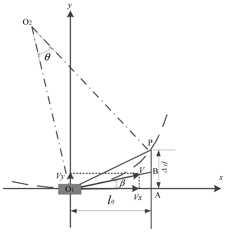
Assuming that the vehicle is moving in a steady state under nonlimiting conditions, first select an appropriate preview distance, and then the image processing module calculates the distance (lateral deviation) between the preview point and the corresponding point of the desired trajectory center. Then, the optimal expected front wheel angle is derived according to the obtained lateral deviation and the vehicle dynamics model, and finally the required front wheel angle (control quantity) calculated by the lateral motion control is used to control the vehicle to follow the desired path. The above process is the best preview control theory. Taking into account the low-speed motion characteristics of the AGV studied in this article, the motion state of the car in the future for a period of time can be regarded as the steady-state motion under nonlimiting conditions, as shown in Figure 5.

As shown in Figure 5, xO₁y is the vehicle coordinate system, point O₁ is the current vehicle centroid position, l₀ is the preview distance, point A is the x-axis coordinate of the preview position determined according to the preview distance, P is the combination of the x coordinate of point A and the image position of the preview point determined by the y-coordinate obtained after recognition, β is the side slip angle of the vehicle’s center of mass, Δd is the lateral deviation of the vehicle and the target trajectory centerline, and O₂ is the intersection of the vertical line of the resultant velocity v and the vertical line of O₁P.

Assuming that within time t_p, the car makes a steady circular motion and travels from the starting point O₁ to the target point P at a yaw rate, its trajectory can be regarded as an arc with O₂ as the center of the arc and R as the radius O₁P.

The speed v of the vehicle can be decomposed into longitudinal speed v_x and lateral speed v_y:

$$v=\sqrt{v_x{}^2+v_y{}^2}.$$

(8)

If t_p is the preview time, then the longitudinal distance $x_{o_{1}p}$ traveled by the car can be expressed as follows:

$$x_{O_{1}P}=v_x{t}_p.$$

(9)

In the steady state of the car, the longitudinal speed v_x of the car can be considered to be much greater than the lateral speed v_y [34]. Under this condition, the vehicle can be regarded as traveling along a circular arc with a radius of R. Under this condition, the steady-state yaw rate w_d is shown by the following formula [35]:

$${\omega }_d=\frac{\theta }{t_p}.$$

(10)

The direction of the vehicle’s total speed v is tangential to the arc, and values of∠PO₁B and ∠PO₂O₂ can be obtained according to the geometric relationship:

$$\angle P{O}_{1}B=\frac{1}{2}\angle P{O}_2{O}_1=\frac{\theta }{2}.$$

(11)

The ∠PO₁A of the right triangle in Figure 5 can be represented as follows:

$$\angle P{O}_{1}A=\frac{\theta }{2}+\beta .$$

(12)

According to the geometric relationship, the relationship with ∠PGC, the right-angled side PC, and the right-angled side OC can be derived as follows:

$$\tan (\angle PGC)=\frac{y_{GP}}{x_{GP}}=\frac{\mathsf{\Delta }f}{v_x{t}_p}.$$

(13)

Combining the above formulas, the value of the angle θ of rotation around the steering center can be obtained:

$$\theta =2\arctan (\frac{\Delta d}{v_x{t}_p})-2\beta .$$

(14)

Substituting Equation (14) into Equation (10), the ideal yaw rate can be expressed as the following equation:

$${\omega }_d=\frac{2\arctan (\frac{\Delta d}{v_x{t}_p})-2\beta }{t_p}.$$

(15)

The vehicle’s center of mass slip angle is the angle between the direction of the vehicle’s center of mass velocity and the front of the vehicle. Since the AGV often travels at low speeds, there is basically no risk of “sideslip, drift”, etc., so the center of mass slip angle can be approximated to 0. Therefore, the ideal yaw rate can be simplified as follows:

$${\omega }_d=\frac{2\arctan (\frac{\Delta d}{v_x{t}_p})}{t_p}.$$

(16)

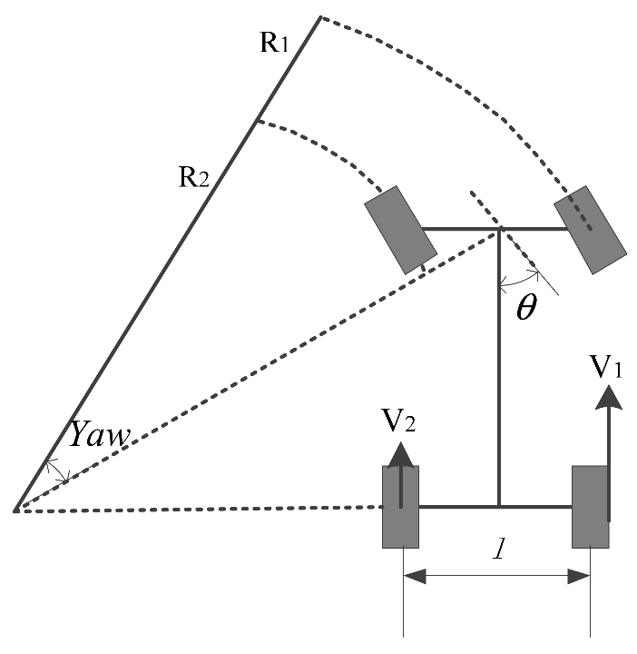
After the desired yaw rate is calculated, the current actual yaw rate needs to be estimated, as shown in the Figure 6.

This article estimates based on the wheel speed difference method, and the final actual yaw rate can be calculated by the following formula:

$${\omega }_r=\frac{v_1-v_2}{l\cos ({\delta }_f)},$$

(17)

where v₁ is the outer wheel speed, v₂ is the inner wheel speed, l is the track, and δ_f is the actual front wheel rotation angle.

Assuming that the vehicle is steering in a steady state with a small steering angle, the dynamics equation of the vehicle are as shown in the following equation [36]:

$$\left\{\begin{array}{c}m{\dot{v}}_y+m{v}_x\gamma =F_{yf}+F_{yr}\\ I_z\dot{\omega }=a{F}_{yf}-b{F}_{yr}\end{array}\right..$$

(18)

In Equation (18), m represents the mass of the whole vehicle; v_x and v_y represent the longitudinal speed and lateral speed of the vehicle when driving, respectively; ω represents the yaw rate of the vehicle; l_f and l_r represent the distance from the front and rear wheels to the center of mass of the vehicle, respectively; F_yf and F_yr represent the lateral force of the front and rear wheels, respectively; and I_z is the moment of inertia at the center of mass of the vehicle. When the vehicle is in a nonlimiting condition, the tire is in the linear region. At this time, the relationship between the lateral force and the tire can be approximately expressed as follows:

$$\left\{\begin{array}{c}{F}_{yf}\approx {\alpha }_f*C_f\\ F_{yr}\approx {\alpha }_r*C_r\end{array}\right..$$

(19)

The slip angle of the front and rear wheels of the vehicle can be expressed as follows:

$$\left\{\begin{array}{l}{\alpha }_f\approx \frac{v_y}{v_x}+\frac{a\omega }{v_x}-\delta \\ {\alpha }_r\approx \frac{v_y}{v_x}-\frac{b\omega }{v_x}\end{array}\right..$$

(20)

The side slip angle of the center of mass when the vehicle is turning at a small angle can be expressed as: $\beta =\frac{v_x}{u}$. Using Equations (18)–(20), we can get an equation for the first-order differential relationship between the yaw rate w and the side slip angle β of the center of mass:

$$\left\{\begin{array}{c}\dot{\omega }=\frac{l_f{}^2{C}_f+l_r{}^2{C}_r}{I_z{v}_x}\omega +\frac{l_f{C}_f-l_r{C}_r}{I_z}\beta -\frac{l_f{C}_f}{I_z}\delta \\ \dot{\beta }=(\frac{l_f{C}_f-l_r{C}_r}{M{v}_x^2}-1)\omega +\frac{C_f+C_r}{M{v}_x}\beta -\frac{C_f}{M{v}_x}\delta \end{array}\right.,$$

(21)

where C_f and C_r are the cornering stiffness of the front and rear wheels, respectively.

For an uncertain system, when both external disturbance and internal parameter perturbation are considered, the system state equation can be expressed as follows:

$$\dot{x}=\Delta Ax+\Delta B[u(t)+E(t)],$$

(22)

where ΔA and ΔB is the parameter perturbation within the system, E(t) is the disturbance including the uncertainty of the system and the external interference, x is the state quantity, and u is the control quantity.

According to Equation (22), we can get:

$$x=\left[\begin{array}{l}\omega \hfill \\ \beta \hfill \end{array}\right],\hspace{1em}A=\left[\begin{array}{c}{a}_{11} a_{12}\\ a_{21} a_{22}\end{array}\right],\hspace{1em}B=\left[\begin{array}{l}{b}_{11}\hfill \\ b_{21}\hfill \end{array}\right],$$

(23)

where

$a_{11}=\frac{a^2{C}_f+b^2{C}_r}{I_{z}v}$, $a_{21}=\frac{a{C}_f-b{C}_r}{M{v}_x^2}-1$, $a_{12}=\frac{a{C}_f-b{C}_r}{I_z}$, $a_{22}=\frac{C_f+C_r}{M{v}_x}$, $b_{11}=\frac{a{C}_f}{I_z}$, $b_{21}=\frac{C_f}{M{v}_x}$.

According to the above formula and combined with the controlled system studied in this article, the state equation is as shown in the following formula:

$$\dot{x}=f({\omega }_r,\beta )+b_{11}[u(t)+E(t)],$$

(24)

where f(w_r) can be expressed by the side slip angle of the center of mass and the yaw rate:

$$f({\omega }_r,\beta )=a_{11}{\omega }_r+a_{12}\beta .$$

(25)

The gain value of the sliding mode control reaching law is:

$$K(t)=\max (\left|E(t)\right|)+\eta ,$$

(26)

where η > 0.

Because it is not possible to directly control the center of mass slip angle, and under normal circumstances, when the vehicle is unstable, the ideal value and the actual value of the center of mass slip angle will produce a large error, the yaw rate is more reflective than the wheel angle of the vehicle as a whole. Therefore, the difference between the actual yaw rate and the ideal yaw rate is selected as the tracking error of the system:

$$e={\omega }_r-{\omega }_d,$$

(27)

where w_d is the ideal yaw rate and w_r is the actual yaw rate. One can design the sliding surface (switching surface) of the controller as follows:

$$s=e+\lambda {\displaystyle \underset{0}{\overset{t}{\int }}e(t)dt}.$$

(28)

One can derive the switch function as follows:

$$\dot{s}=\dot{e}+\lambda e={\dot{\omega }}_r-{\dot{\omega }}_d+\lambda \left({\omega }_r-{\omega }_d\right).$$

(29)

The sliding mode control law is designed as follows:

$$u=\frac{1}{b_{11}}[-f({\omega }_r)+{\dot{\omega }}_d+\lambda ({\omega }_r-{\omega }_d)+K(t)\mathrm{sgn}(s)].$$

(30)

To prove the stability of the initially designed sliding mode controller, the Lyapunov function is as follows:

$$V=\frac{1}{2}{s}^2,$$

(31)

which is derived as follows:

$$\dot{V}=s\dot{s}=s[\dot{e}+\lambda e]=s[f({\omega }_r)+b_{11}[u(t)+E(t)]+{\dot{\omega }}_d+\lambda e].$$

(32)

Substituting the sliding mode control law of Equation (31) into Equation (33), we get:

$$\dot{V}=s[-K(t)\mathrm{sgn}(s)-E(t)]=-K(t)\left|s\right|-E(t)s\le -\eta \left|s\right|\le 0,$$

(33)

where η > 0, so the designed control law meets the stability requirements.

Substituting this into Equation (29) produces the following equation:

$$\dot{s}=\frac{l_f{}^2{C}_f+l_r{}^2{C}_r}{I_{z}v}{\omega }_r-\frac{l_f{C}_f}{I_z}\delta -{\dot{\omega }}_d+\lambda ({\omega }_r-{\omega }_d),$$

(34)

where w_r and w_d can be obtained by formula x and formula y, respectively. Let $\dot{s} = 0$; since the vehicle is moving in an approximately uniform circular motion at this time, the yaw angular acceleration ${\dot{w}}_d=0$, so the control variable front wheel angle can be expressed as follows:

$$\delta =\frac{I_z}{l_f{C}_f}[\frac{l_f{}^2{C}_f+l_r{}^2{C}_r}{I_{z}v}{\omega }_r+{\lambda }_0({\omega }_r-{\omega }_d)].$$

(35)

According to the sliding mode control law,

$${\delta }_d=\delta +K(t)\mathrm{sgn}(s).$$

(36)

The switching coefficient K(t) determines the speed at which the moving point not on the sliding surface approaches the sliding surface. The larger the K(t), the faster the moving point approaches the sliding surface, which is the response of the control. The faster it is, the poorer the steady-state convergence, which will cause more jittering; if K(t) is smaller, the speed of the moving point approaching the sliding mode surface is slower, and the dynamic convergence is poorer. The jitter of sliding mode control is mainly caused by the approach term K(t)sgn(s), so it is necessary to limit the jitter phenomenon of the sliding mode controller. In this paper, a fuzzy controller with variable universe is designed to adjust the switching gain coefficient K(t).

According to Equation (36), although the existence of the sign function can effectively eliminate the unknown interference, it inevitably leads to chatter. The main drawback of the chatter phenomenon has been solved to a certain extent through the use of FSMC, which has become more common. Compared with various types of deep learning algorithms such as neural networks, fuzzy control has excellent adaptive approximation and no need for precise prior knowledge, which makes it easier to be widely used. Therefore, this paper adopts adaptive fuzzy control based on switching fuzzification to improve the trajectory of the system near the sliding mode surface, which not only enables the system to adapt to various working conditions, but also leads to better elimination of different interference intensities, so through fuzzy approximation the continuity of the discrete sign function can effectively reduce chatter.

The variable switching gain designed in this paper uses fuzzy rules to adjust the switching gain according to the relative position and movement trend of the system and the sliding mode surface.

Taking S and $\dot{S}$ as the fuzzy input quantity and k as the output quantity, the corresponding fuzzy language variables are {NB NM NS ZO PS PM PB}. If $S\dot{S}$> 0, the current state of the sliding mode function is the same as the change trend, and there is a trend away from the sliding mode surface. At this time, the switching gain k(t) should increase. If $S\dot{S}$ < 0, the system is already approaching the sliding mode surface, and the switching gain k should be reduced. At the same time, the size of |$S\dot{S}$| also needs to be considered to further rationally design fuzzy rules. When |$S\dot{S}$| is large, |k| should also have a large amount of change, and vice versa.

In the design of a fuzzy controller, the design of fuzzy rules is an important part of determining its performance. This article gives 49 fuzzy rules for the switching gain coefficient k(t) in

Table 1. Fuzzy rule table [37].

		s
		NB	NM	NS	ZO	PS	PM	PB
ds	NB	NB	NB	NM	ZO	PM	PB	PB
	NM	NB	NM	NS	ZO	PS	PM	PB
	NS	NM	NS	NS	ZO	PS	PS	PM
	ZO	ZO	ZO	ZO	ZO	ZO	ZO	ZO
	PS	PM	PS	PS	ZO	NS	NS	NM
	PM	PB	PN	PS	ZO	NS	NM	NB
	PB	PB	PB	PM	ZO	NM	NB	NB

:

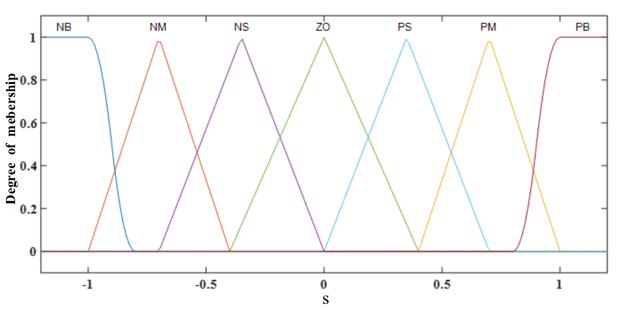
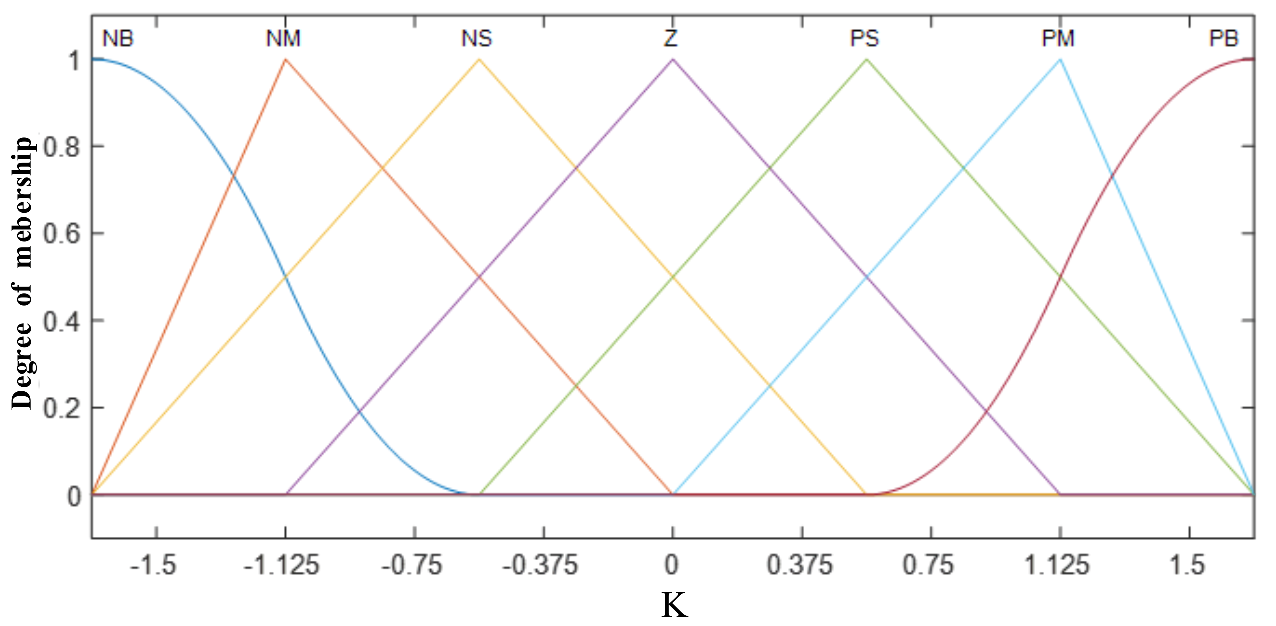
According to the above fuzzy rules, the corresponding relationship between the two input and output fuzzy sets and their quantity range are shown in Figure 7:

This paper uses a product inference engine, a single value fuzzer, and a center average defuzzer. The output y(x) of the fuzzy system can be written as follows:

$$y(\mathrm{x})=\frac{{\displaystyle \sum _{j=1}^m{y}^j({\displaystyle \prod _{i=1}^n{\mu }_{A_i^j(x_i)}})}}{{\displaystyle \sum _{j=1}^m({\displaystyle \prod _{i=1}^n{\mu }_{A_i^j(x_i)}})}}.$$

(37)

In this section, the switching function s(t) is used as the input of the fuzzy system, where ${ A}_i^j$ is a fuzzy set, ${\mu }_{A_i^j{(x}_i)}$ is a fuzzy set is the membership function of s_i, the Z-type membership function is used by μ_NB, the S-type membership function is used by μ_PB, and the rest of the fuzzy variables are all triangular membership functions. The initial membership function is shown in the Figure 8, Figure 9 and Figure 10:

According to the principle of fuzzy control, in order to make a fuzzy system infinitely and accurately approximate a changing function, in theory, it needs an infinite number of fuzzy rules to realize it, which is almost impossible to achieve. Also, when setting the fuzzy domain interval, the initial domain interval is difficult to choose. Therefore, a more accurate approximation can be achieved through adaptive adjustment of the universe under the premise that the number of rules and the membership function remain unchanged.

According to the abovementioned fuzzy controller design, the input and output domains are scaled and adjusted. This paper uses the exponential expansion factor in the function model to adaptively adjust the fuzzy universe of three variables:

$$\alpha (x)=1-\lambda {\mathrm{e}}^{(-0{.5*\mathrm{x}}^2)}\lambda \in (0,1),$$

(38)

where x is the input variable of the controller and λ is the scale factor, which determines the degree of scaling. After repeated trials and adjustments, the expansion factor λ of the input domain in this article is 0.6, and the expansion factor λ of the output domain is 0.3.

Due to the introduction of the expansion factor of the input and output domains, the initial domain designed in the previous paragraph needs to be adjusted according to the expansion factor, so that the product of the adjusted domain and the expansion factor $\alpha \left(x\right)$ is centered on the initial domain.

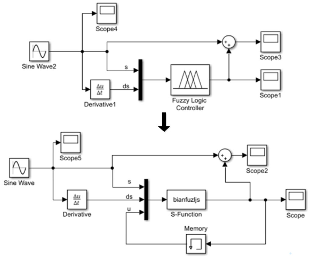
Since the fuzzy logic module in Matlab/Simulink cannot realize the variable universe, we used the S-function function to replace the original fuzzy logic module, as shown in Figure 11. It can be seen that the variable universe FSMC has added a feedback link, and the controller output (control quantity) at the previous moment is used as the independent variable of the variable universe expansion factor. The variable domain can adjust the corresponding fuzzy domain according to the actual input and output range, and the domain can be expanded in time when the output control quantity increases, so that the control quantity is not restricted by the maximum domain scope, and it is enough to ensure the stability of the system. When the output control quantity becomes smaller, the time shrinkage within the universe increases the control accuracy, guarantees the steady-state convergence, and finally realizes more precise and rapid control.

6. Construction of Vision-Guided AGV Test Platform and Real Vehicle Tests

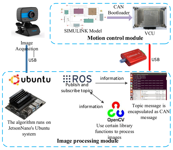
The software implementation is divided into two parts. The upper image processing algorithm is developed based on the ROS framework. Messages are transmitted between different nodes through topic publishing and subscription. The upper layer packages the final calculated key variables as topic messages, and then packages some topic messages (such as navigation deviation) as can messages and sends them to the CAN bus for VCU to read and call. The core code of image preprocessing, leader extraction algorithm, and topic message of each node are written in C++ and Python, and some library functions in OpenCV library are used to complete the image processing work. The lower motion control is based on the rapid prototyping development method; this uses Matlab/Simulink to build the motion control algorithm, generates the automatic code, and finally burns the program into VCU. The overall architecture of the software system is shown in Figure 12.

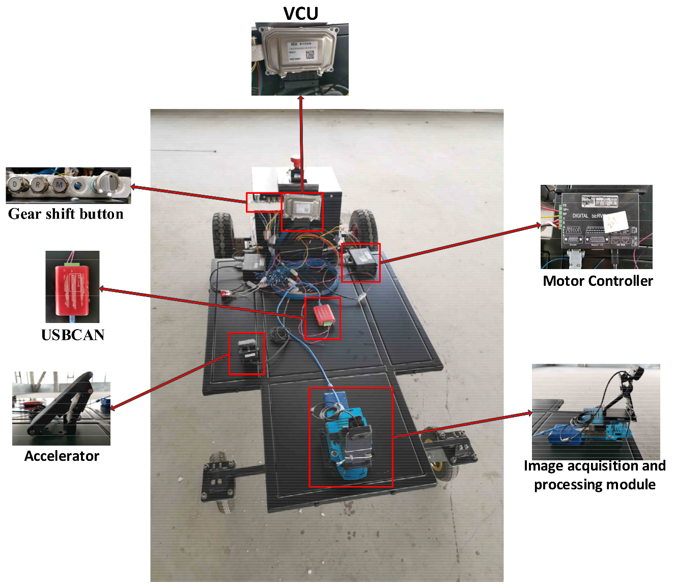
The hardware system of vision-guided AGV mainly includes a body, power supply, vision system, motion control module, and manipulation module. The test chassis is a 1/4 mini vehicle model, with length * width of 1.2 m * 0.6 m; considering the safety in the test stage, the maximum speed is 2 m/s. The power supply is a 24 V lithium iron phosphate battery, the motor is a servo motor with rated power of 400 W, the lower controller is a 24 V vehicle controller (VCU) with slow charge wake-up and can wake-up, the upper controller is the Jetson Nano product of NVIDIA, and the camera is a UVC drive-free camera head. Among the above components, the VCU and motor are powered by a 24 V battery pack, the image processing module is powered by a separate 12 V power supply, and the image acquisition module is powered by USB. The vision system mainly includes an image acquisition module (camera), an image processing module (host), etc. The number of camera pixels is 640 * 480 and the number of frames is 30 fps. With this number of frames, insufficient image processing speed will lead to abnormal vehicle driving. The motion control module mainly includes a vehicle controller, drive motor, motor controller, etc. The connection or communication mode between the above modules is shown in Figure 13. The camera provides system input by collecting the front path image, and is connected with the image processing module through USB. The image processing module processes the collected images in real time, uses the usbcan tool supporting Ubuntu system to send the calculated navigation deviation to the CAN bus through the CAN bus, reads the can message by the VCU, completes the motion control by the VCU, sends the left and right desired speeds to the motor controller through the can, and finally completes the drive control of the motor by the two motor controllers. This drives the Automatic Guided Vehicle (AGV) to follow.

The whole hardware layout is shown in Figure 13.

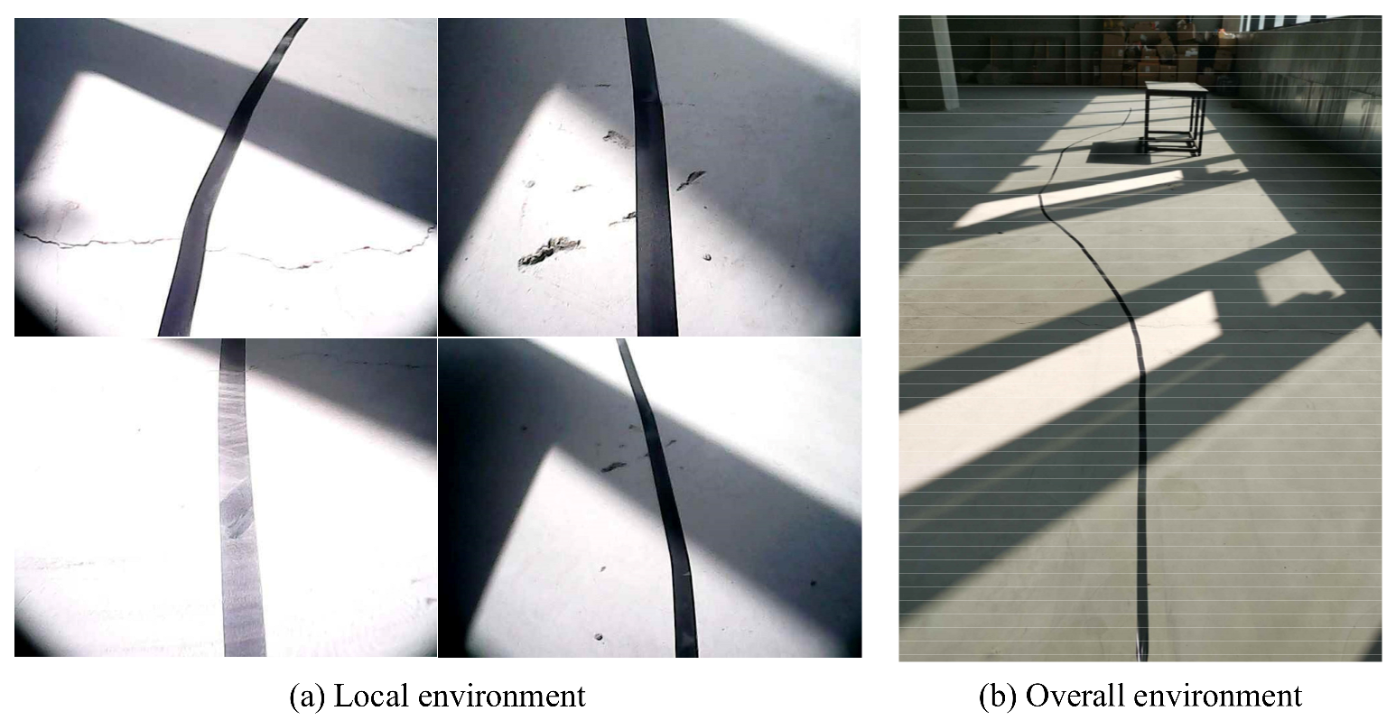
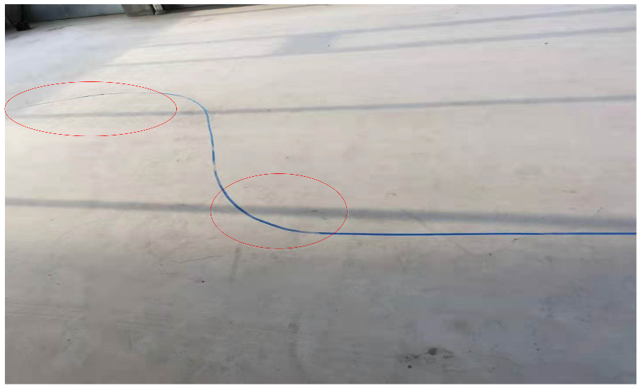
In this paper, a real vehicle test is carried out in a warehouse scene. In order to verify the operation effect of the algorithm designed in this paper under extreme conditions, interference items are added to the existing scene, such as selecting the area with strong light and dark contrast for testing, adding messy lines on the ground, etc. The test scenario after layout is shown in Figure 14.

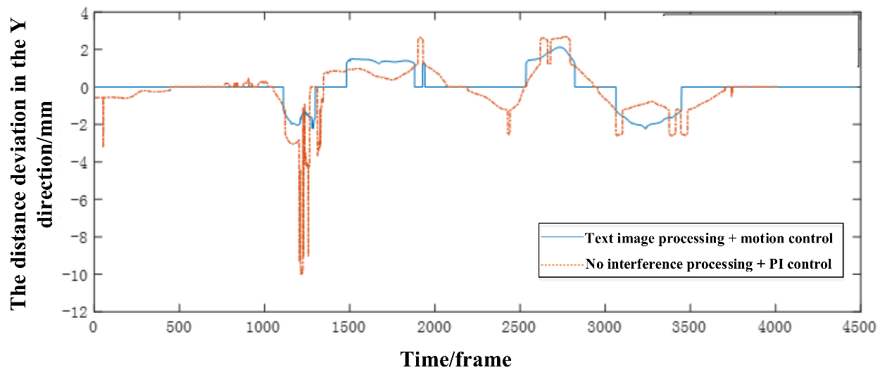
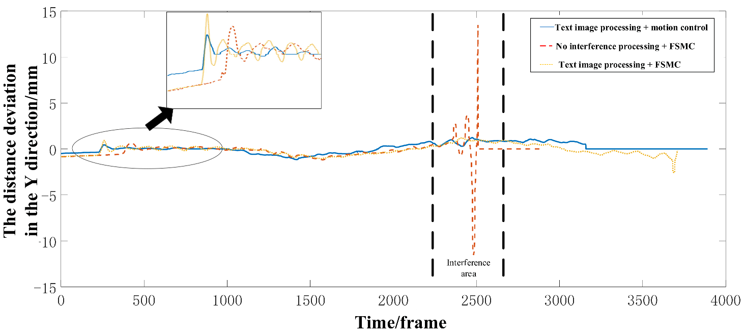
In this paper, a width range of 15 pixels is regarded as 0 error during the test. The test results in this scene are shown in Figure 15.

In Figure 15, the Y-axis is the deviation in distance between the center line of the vehicle and the center of the guide wire, the X-axis is the number of frames of image acquisition, and the test route is approximately a single moving line. The motion control algorithms used are variable universe fuzzy sliding mode control designed in this paper. In terms of image processing, non-interference processing is used to compare with the image processing algorithm in this paper. The image recognition method without anti-interference processing has no preprocessing, and uses traditional canny edge detection to extract the guide wires. Therefore, this comparison can reflect the stability and reliability of the image recognition algorithm designed in this paper. After the image preprocessing algorithm and guide line extraction algorithm designed in this paper, the preview points basically fall on the guide line. Only a few frames of small-scale error recognition appear in the interference area, which is reflected in the driving error curve—that is, there are limited times of small-scale jump, and the rest drive stably along the guide line. The leader recognition algorithm without anti-interference processing has poor performance obtaining the preview point, and is very vulnerable to the external environment. As shown in Figure 15, although the preview point will not deviate from the guide line in the area with uniform illumination, the preview point frequently deviates from the guide line after entering the interference area, resulting in a continuous jump of the calculated navigation error, which seriously interferes with the normal driving of AGV.

In order to comprehensively show the actual control effect of the image processing algorithm and motion control algorithm designed in this paper, another group of comparative tests are carried out on the test route of approximate double shift line, as shown in Figure 16. The parameters of PI control are determined after repeated debugging, and a set of optimal parameters is determined based on the weighted sum of deviation variance and average deviation. Firstly, a series of anti-interference image processing algorithms and variable universe fuzzy sliding mode control algorithm are used for testing. It can be seen that there is no error jump in the whole test process; the following can be completed quickly when there is a curve ahead, and the maximum error is within ± 2 mm in the whole test process. After that, the guide wire identification algorithm without anti-interference processing and PI control are used to test the same site. There is a large continuous jump at the first bend, and there are many false identifications in the whole test process, resulting in more sudden changes and a large amplitude of driving error. In terms of motion quality, the steady-state accuracy is lower than that of variable universe FSMC, which is difficult to maintain stably. The transient characteristics are also poor, the stabilization time is longer than that of the variable universe FSMC, and the PI control parameters need to be continuously adjusted according to the actual operating environment, so it is difficult to use the same set of parameters to deal with all scenarios, while the variable universe FSMC can adapt to various working conditions without manual adjustment, which is convenient for layout and use in different scenarios.

In order to test the control effect of the motion control algorithm under a large curvature path and the identification under the condition that the guide wire is not obvious, another comparative test is also carried out on the scene shown in Figure 17. The guide route is “S-bend,” the interference area in the route has local pollution and line interference, and there is uneven illumination or strong light reflection in some sections.

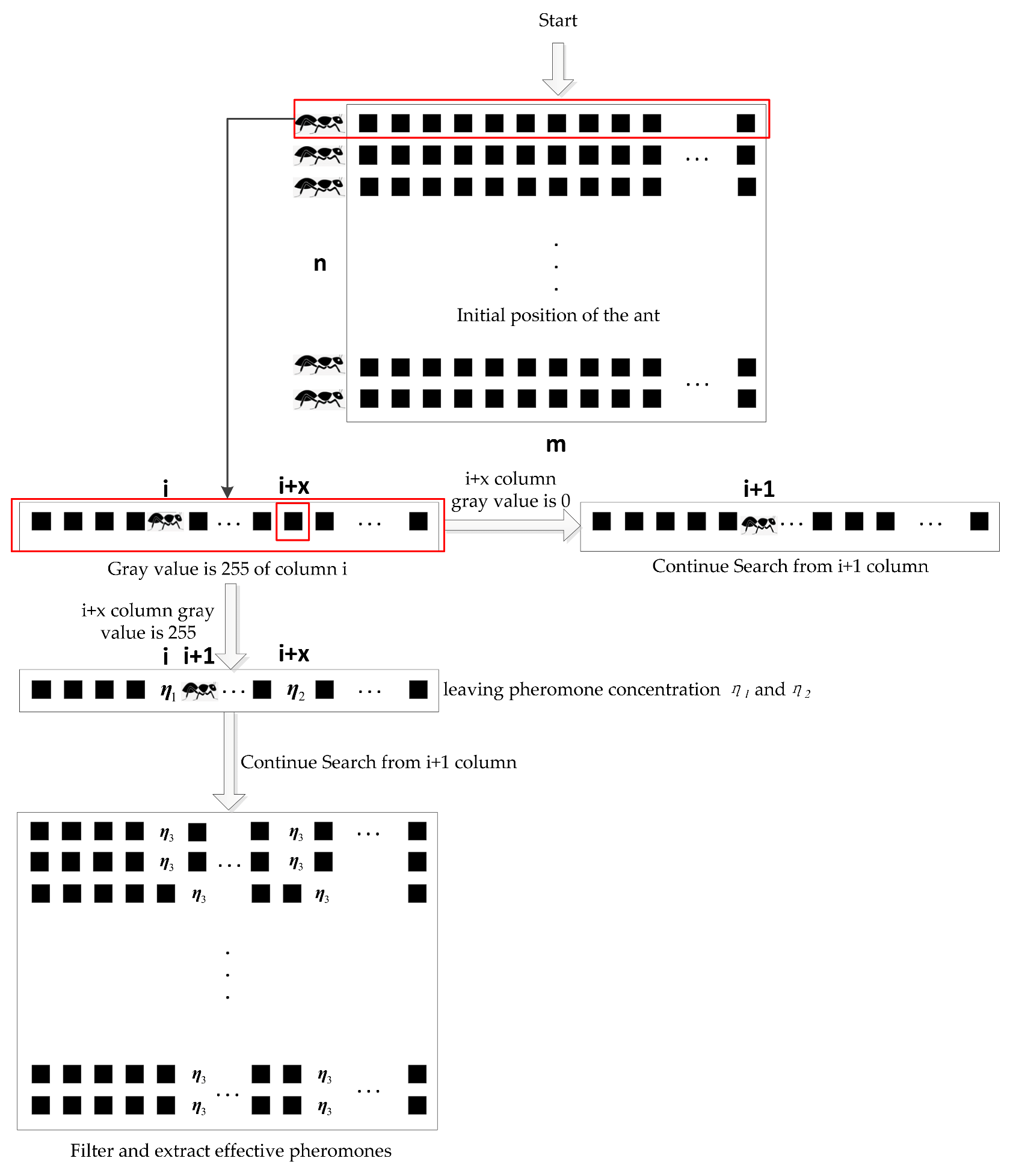
In this scenario, the FSMC algorithm is first used to compare with the variable universe FSMC algorithm designed in this paper. It can be seen from Figure 18 that, when a large area rate curve appears in front, it is equivalent to giving a pulse to the sliding mode system. When the error suddenly appears, the response of the variable universe FSMC is not only faster, but also quicker to limit the error. Moreover, it can further reduce the frequency and amplitude of chatter based on FSMC, and further improve the motion quality of AGV. After the 3000th frame of the experiment, the FSMC algorithm has a large steady-state error and finally fails to converge to the zero deviation position. Due to the timely adjustment of the scope of the universe, the variable universe FSMC algorithm can quickly and accurately converge to the steady state and maintain this state. Secondly, in this scenario, the series of image processing algorithms designed in this paper are verified and compared with the algorithm without anti-interference processing. There are many interferences in the interference area, such as uneven illumination and unclear guide wires. The guide wire identification algorithm without anti-interference processing will have frequent “false identification,” resulting in large left and right yaw of AGV in the interference area, or even interruption in the middle, failing to travel a complete path, seriously interfering with the normal driving of AGV. The ant colony algorithm will fit the qualified broken lines so as to avoid the wrong identification due to the contamination of some lines. At the same time, the preprocessing algorithm designed in this paper can deal with the impact of uneven illumination and ensure the correct identification of guide wires.

It can be seen from

Table 2. Comprehensive performance test results.

Route	Carrying Algorithm	Maximum Deviation (mm)	Variance of Deviation (mm2)
Route shown in Figure 15	Image processing algorithm with variable universe FSMC	2.0125	0.5345
	No anti-interference processing with variable universe FSMC	8.0625	1.1658
Route shown in Figure 16	Image processing algorithm with variable universe FSMC	2.2375	0.7763
	No anti-interference processing with PI control	10.0500	1.7424
Route shown in Figure 18	Image processing algorithm with variable universe FSMC	1.2000	0.2688
	No anti-interference processing with FSMC	13.5	1.0783
	Image processing algorithm with FSMC	2.5750	0.3087

that, in the single line shifting test shown in Figure 15, when the motion control algorithms are the same and both are equipped with variable universe FSMC, the deviation in the driving process is significantly reduced. After the image processing algorithm designed in this paper, the maximum deviation is only 2.0125 mm and the variance of the deviation is 0.5345 mm², compared with 6.05 mm and 0.6313 mm², respectively, for the noninterference processing algorithm. The significant reduction of the maximum deviation shows that the image processing algorithm designed in this paper does not have the wrong identification of the preview point when encountering external interference, and can make the preview point located on the guide line as much as possible. The reduction of deviation variance shows that preview point is rarely deviated from the guide line. Compared with the noninterference processing algorithm, the deviation false detection frequency of preview point is greatly reduced.

In the double shift line test shown in Figure 16, when the series of algorithms designed in this paper are used for image processing and motion control, compared with noninterference image processing and PI motion control, the maximum deviation is reduced by 7.8125 mm and the variance of deviation is reduced by 0.9661 mm². After the algorithms designed in this paper are used for the upper and lower algorithms, the actual motion effect of AGV changes more significantly. The stability of the Automatic Guided Vehicle (AGV) tracking process is greatly improved, and the amplitude and frequency of driving deviation are reduced. The experiment shows that the error accumulation of each link will eventually lead to the infinite amplification of the final error, which will greatly affect the normal operation of AGV.

In the “S-bend” route test shown in Figure 18, when the series of algorithms designed in this paper is used for image processing and motion control, compared with the replacement of motion control with FSMC, the maximum deviation is reduced by 1.375 mm and the variance of deviation is reduced by 0.0399 mm², indicating that we have further effectively improved the control accuracy and motion quality on the basis of the FSMC algorithm. Using a noninterference image processing algorithm combined with a FSMC motion control algorithm, there is a large range of continuous fluctuation in the interference area, resulting in a maximum deviation of 13.5 mm and a variance of deviation of 1.0783. Therefore, anti-interference image processing and high-precision motion control under visual navigation scheme are necessary, and the above algorithm designed in this paper has been greatly improved.

7. Conclusions

With the increasing requirements for automation and intelligence in today’s society, Automatic Guided Vehicles (AGV) will play a more and more important role in efficient automatic transportation. The visual guidance mode has gradually become one of the most important and popular perception modes. In order to ensure that Automatic Guided Vehicles (AGV) can continue to drive stably according to guide lines in extreme cases such as uneven illumination, line interference, and unclear or even damaged guide lines, and to improve the motion quality and robustness of visual guidance AGV, this paper focused on the difficulty of accurately extracting the guide wire when a vision-guided AGV runs in a complex working environment, and explored the applications of machine vision technology in the field of AGV. Navigation deviation and lateral motion control were also studied, providing a new method and ideas for the further development of vision-guided AGV from the two aspects of image recognition and motion control.