Abstract
Penetration of renewable energy resources in modern power systems has increased rapidly. The integration of different renewable and nonrenewable resources for the purpose of electricity generation is referred to as Distributed Generation (DG) units. The penetration of DG units gave birth to the concept of power microgrid. Power inverters play a major role in the integration of DGs in the power system. Control and stability analysis of microgrids in power systems is a challenging task for the control community. Dynamic microgrid modeling demands knowledge of fundamental engineering laws to detailed theoretical analysis. To model the dynamic behavior of the power microgrid, a basic understanding of the power converter operation modes and their control schemes is necessary. The main microgrid modeling components are power converters, power lines, transformers, protection systems, load, and faults. In this paper, preliminary concepts of power systems along with graph theoretic approach are used to develop the model of the microgrid and main grid networks. A mathematical model of a power microgrid in islanded mode, as well as the grid-connected mode, is developed and comprises of generation sources, power inverter interface, protection mechanism, load, faults, and transmission lines. The developed mathematical model can be used to address the stability issues as well as resilience in the power networks for complete system analysis. To validate the mathematical model, a renewable energy-based main grid and microgrid model is simulated. The graphical result of simulated model presents the generation and load curves.
1. Introduction
Conventional power generation units have environmental disadvantages. To overcome these disadvantages, renewable energy generation is encouraged. Most of the renewable energy generation units are low power as compared to conventional units [1,2]. Therefore, integration of those energy units is done at Low Voltage (LV) and Medium Voltage (MV) levels in the power system. The generation units at such voltage levels are referred as Distributed Generation units (DG) [2,3]. The interface of DGs with the power network is achieved using power inverters. The characteristics of power inverters may vary due to the characteristics of synchronous generators in the power network [4]. Different control and operational strategies are required to integrate and operate DGs in the power network. The power microgrid facilitates the integration of DG units in the power network. Microgrid comprises of generation units, load and energy storage devices at transmission or distribution level in the power network [5,6]. The efficiency of the microgrid in the power network depends on the control mechanism. The control mechanism at the distribution and transmission level is referred to as the local control or is commonly known as decentralized or distributed control [7]. Decentralized control does not share information, such as voltage, frequency, and power, locally, while distributed control shares the information with neighboring units in the power network. This development makes control of the microgrid a challenging task [8,9,10]. To complete this challenging task, it is very important to develop the mathematical model of a microgrid that covers the important aspects and concepts of power systems [11,12,13,14]. The mathematical modeling of a power microgrid can help to address the stability and control challenges [15].
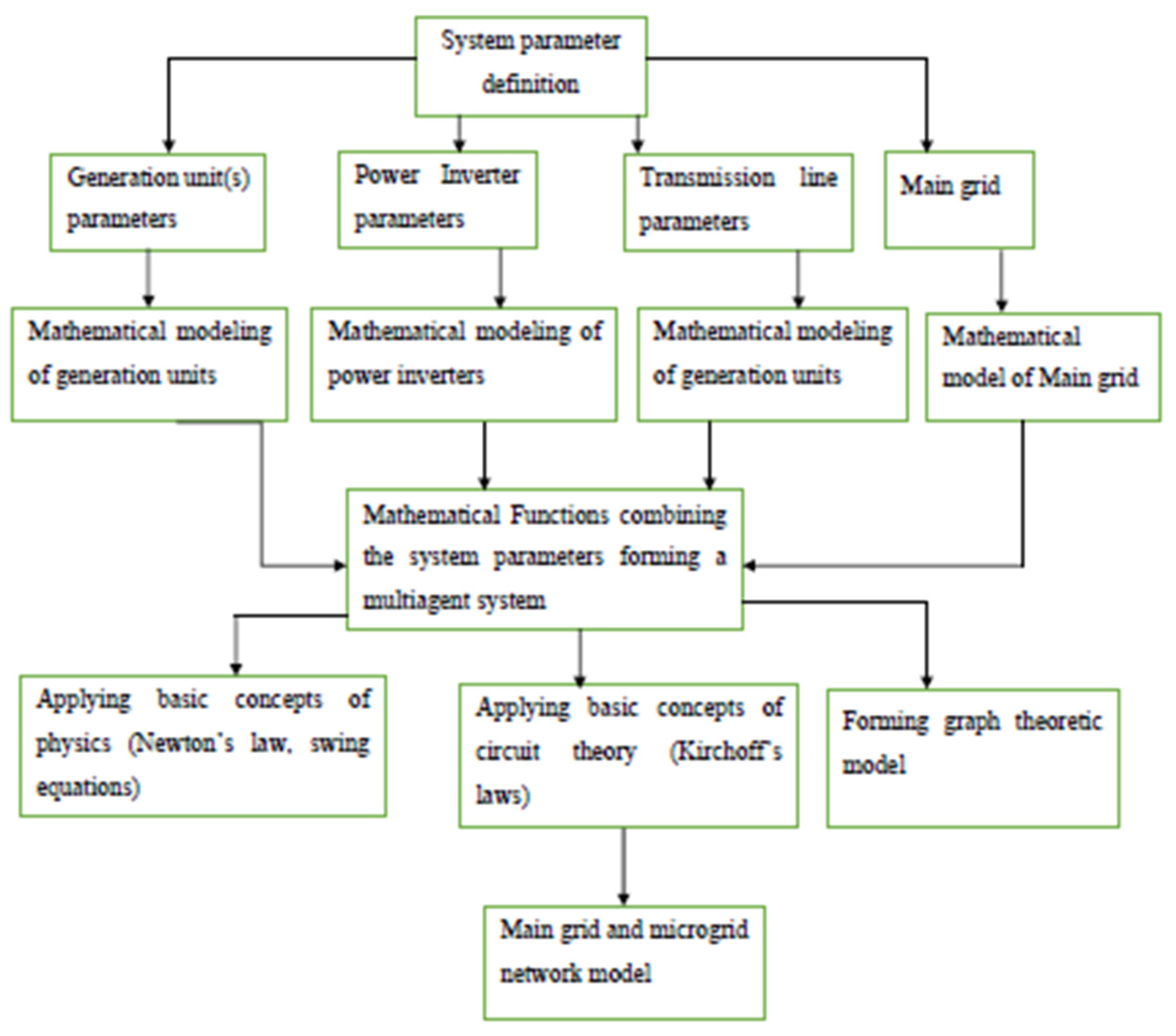
This paper provides comprehensive modeling of the microgrid based on fundamental laws of physics and electrical engineering combined with microgrid components and their operational modes. The role of graph theoretic structures is highlighted to represent the generation, power conversion, transmission and distribution in the power grid networks. Coordinate transformation with singular perturbation argument shows that the power flow model can be obtained from the network with dynamic line models. This paper discusses techniques in modeling and control of inverter interfaced microgrids restricted to individual DG with electrical network interactions in the power network. Model reduction via time scale separation based on the power flow model is also discussed. This paper also emphasizes on the modeling of the electrical network interaction model as a multi-agent system model. A modeling technique to develop a general multi-agent model using distributed control schemes for the stability analysis of power systems will also be discussed in detail. The flowchart representing the overall scheme to model the power network is presented in Figure 1. The novelty in this article is the multi-agent-based modeling of the main grid microgrid network. This network model presents power generation, power transmission, power inverter interface, power protection and energy management. The developed mathematical model represents all the physical components in the network. Using the measurement devices referred to as communication nodes over the physical components will form a cyber layer.
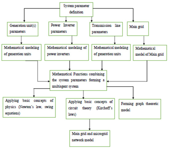
Figure 1.
System modeling scheme.
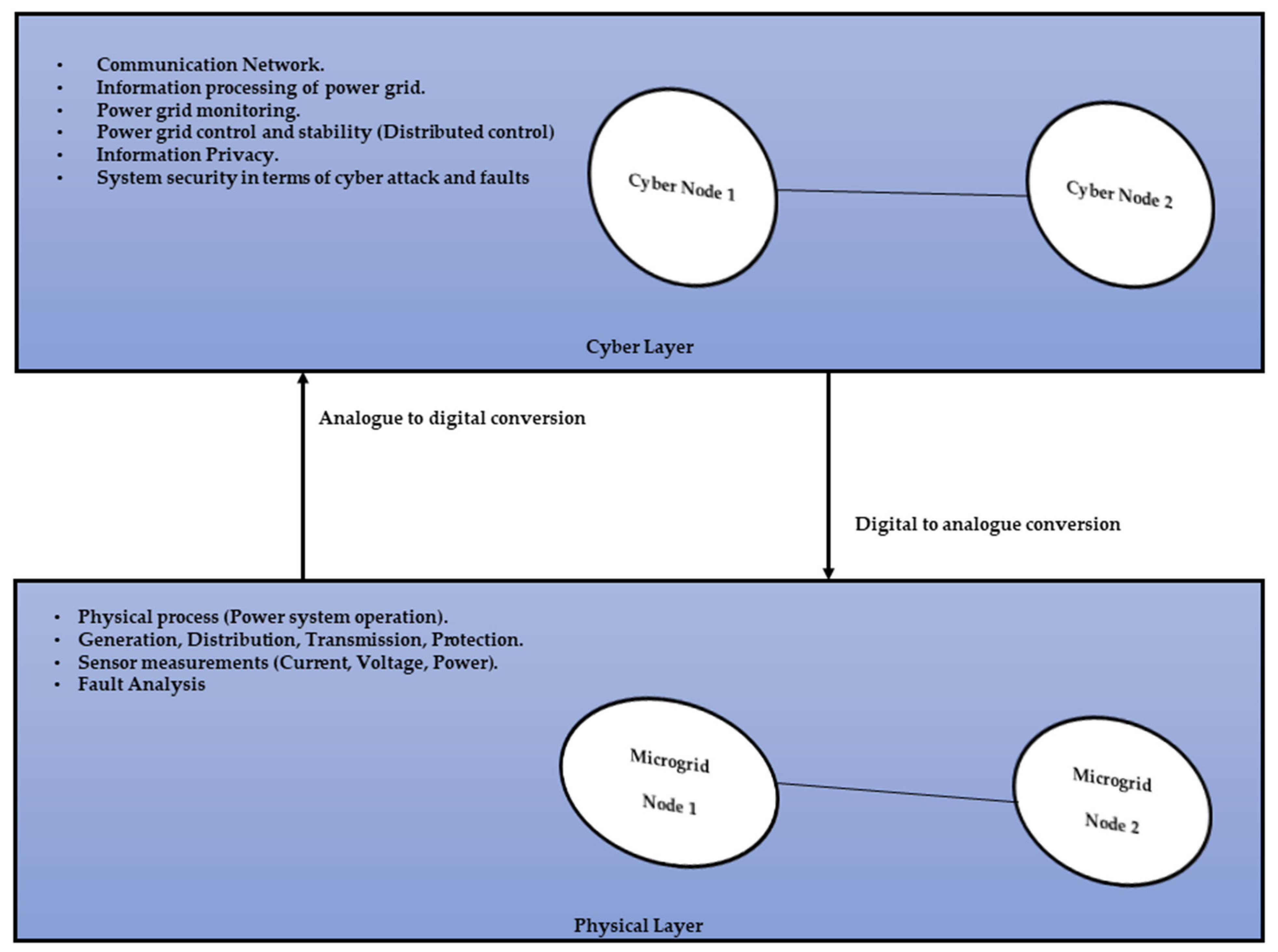
The growing developments in the power grid architecture require advanced control and monitoring platform. The Multi-agent-based cyber-physical systems provide the platform to control and monitor the power grid network. The graph-theoretic architecture is used to model the power systems as a multi-agent system. In the power grid, the conventional generation units and distributed generation resources forming a graph-theoretic network are referred to as nodes and power lines are referred as the edges. The graph-theoretic platform is mainly based on a distributed framework. In this framework, a distributed control is performed for each agent’s synchronization in terms of voltage, frequency, and power. This makes the power grid infrastructure critical in terms of efficiency and stability. The infrastructure gets critical due to the heterogeneous nature of nodes (generation units and power lines) in the physical layer and interconnected communication networks in the cyber layer. The communication network in the cyber layer uses different computational technologies to control and monitor the physical layer.
The integration of the cyber layer in the power network raises several challenges as compared to traditional systems. The complex interconnectivity and interdependency of the cyber layer and physical layer enhance the potential challenges in terms of faults, failures, and security vulnerabilities in the network. These challenges can cause information processing errors (cyber intrusions or system failures) to analyze the complete system. To accommodate the stability and control challenges in the physical layer in case of system fault or failures control techniques like adaptive control, robust control, backstepping control, etc., can be used. To deal with the cyber layer vulnerabilities, the cyber protection mechanism and efficient information processing are required.
To cater such challenges in power networks, a graph-theoretic approach forming a multi-agent network is considered as resilient in terms of stability and control in the physical layer and efficient information processing in the cyber layer. Several distributed control mechanisms may be developed in the multi-agent-based power network to detect and recover from cyber and physical faults. This makes the multi-agent-based power network more flexible. A simplified presentation of a power network as a cyber-physical system is presented in Figure 2.
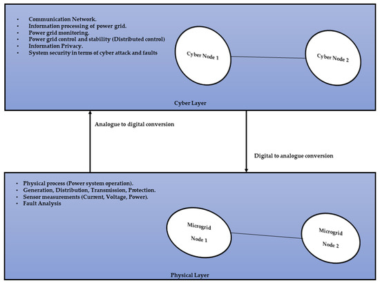
Figure 2.
Multi-agent-based power grid as cyber physical system.
The cyber layer can provide real time power network information. This results in the utilization of the modeled network of power systems as cyber-physical systems. This flow of electric power and information enables the smart grid technologies. Although digital communication in power systems is reliable and efficient, due to the extensive use of renewable energy resources which challenges the resilience in the power network. These challenges require an efficient mathematical model of power network to analyze the complete system. The cyber-physical modeling can represent measurements at power inverter, power distribution and power generation as individual system models. This type of system model can be utilized to address various challenges such as voltage dips, frequency deviations as well as active and reactive power control.
The rest of the paper is organized such that Section 2 presents the basic notations and preliminaries of power systems, multi-agent systems and power microgrids. Section 3 discusses multi-agent system-based modeling of the microgrid in the power network with reference to graph-theoretic analysis. Section 4 (1,2,3,4,5,6) presents dynamical modeling of inverter interfaced microgrid along with the modeling of power lines, transformers, proposed microgrid model constituting inverters, transmission lines, loads, faults and protection systems. A brief review of the control strategies in a power microgrid is also presented in this section. Section 5 reviews the challenges in the power systems stability and control. The paper is concluded in Section 6 with open research questions in the modeling and control of microgrids.
2. Preliminaries and Basic Definitions
2.1. Power Systems
Definition 1.
An AC signal denoted as must satisfy the following properties [16,17,18].
Definition 2.
A three phase AC signal is defined as[16,17,18] such that
where , , ,
Definition 3.
A three phase AC symmetric signal is denoted asand
A three-phase AC signal is said to be asymmetric if it is not symmetric [16,17,18].
Definition 4.
A three-phase AC electrical system is symmetrically configured if symmetrical feeding voltage yields a symmetrical feeding current and vice versa. The system is said to operate under symmetric conditions if it is symmetrically configured and symmetrically fed [17,18].
Definition 5.
For signal/system and then the mapping is defined as:
Then is dq0 transformation such that:
.
Three-phase dq0 transformation simplifies the control design and analysis due to its advantage in mapping the three-phase AC signals to constant signals (periodic signals to constant equilibria). Two quantities can represent a power system operating in symmetric (balanced) mode by applying mapping to dq0 transformation with angle adjustment [16,17,18].
where voltage phase angle,
= adjustment angle in the phase.
The transformation is to referred as the Park transformation
for all for symmetric power system. The dq transformation is represented as:
The above transformation can be applied to three phase symmetric AC system as:
Definition 6.
Three-phase AC power system is either presented as three-phase three-wire (deltanetwork) or a three-phase four-wire (wyenetwork) in the symmetric and asymmetric manner [16,17,18].
Definition 7.
For a three-phase symmetric AC power system the voltage and current are defined as [16,17,18]:
where = curent phase angle.
The dq transformation for voltage and current are defined as:
Definition 8.
Three-phase active, reactive and apparent power is defined on the basis of voltage and current as [16,17,18]:
where = active power;
Q = reactive power;
S = apparent power;
V = voltage;
I = current.
2.2. Algebraic Graph Theortic Model of Power Network
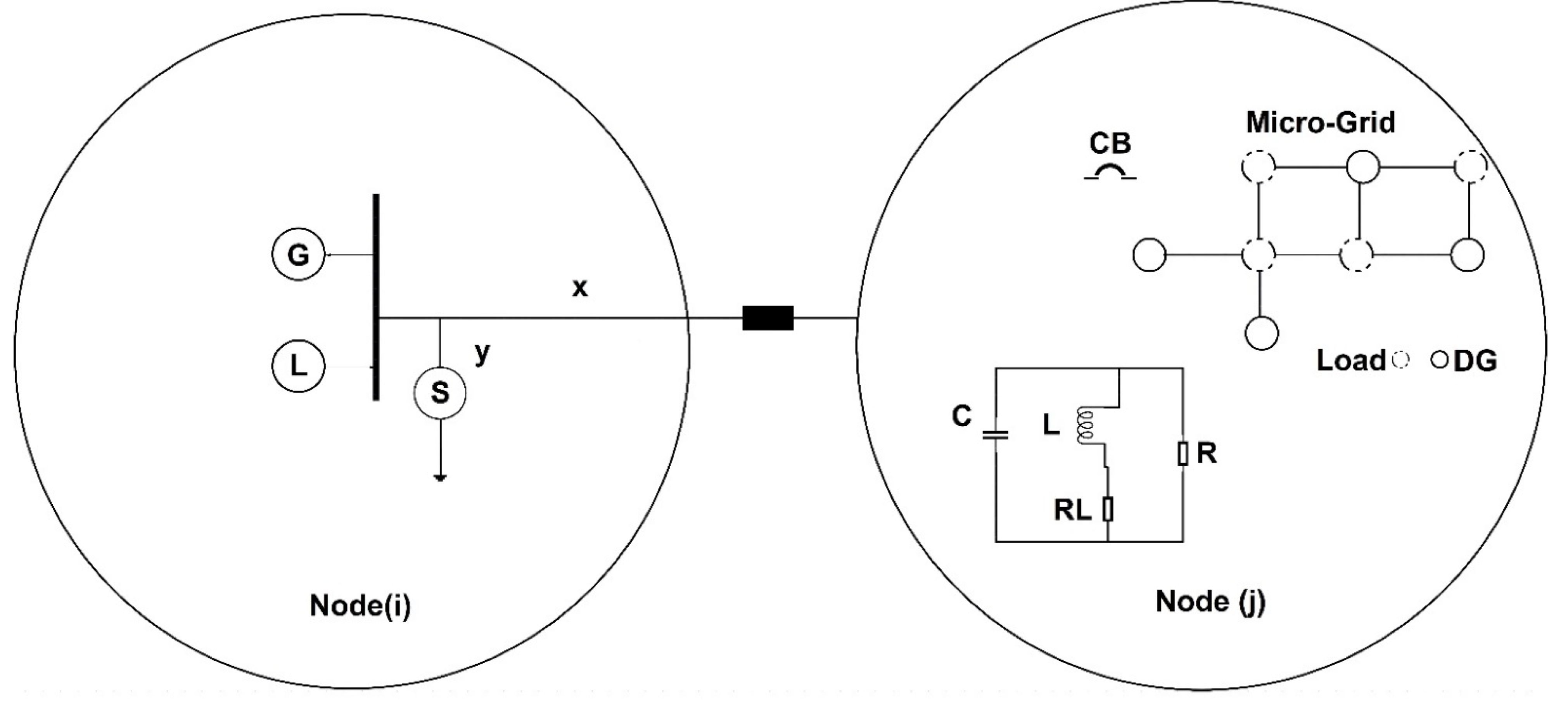
Suppose represents a power microgrid (MG). presents the power nodes and presents power lines. Let present the power microgrid with a connected communication network. presents the communication nodes in the microgrid and presents communication links in the microgrid. In multi-agent system topology, each node presents an agent. For a communication network in a microgrid, the matrix represents the adjacency matrix. The set presents the neighboring nodes of node in the microgrid. The matrix such that presents the diagonal matrix. The Laplacian matrix is defined as . It is assumed that the generator set presents the generator buses and set presents the non-generator buses. The number of generator and non-generator buses are then denoted as and , respectively. The connectivity (edge set) is denoted by . The network topology is considered undirected i.e., for buses connected in the network is the same as . presents the complex phasor voltage of the generator at bus and presents the complex phasor voltage of the bus . presents the complex phasor current and presents the reactance between buses . In the current scenario the nodes in the microgrid present DG, load, protection system and inverter interface. The edges in the current scenario present the power lines (LV or MV lines) [19,20].
Definition 9.
The power, voltage and current flowing from the internal generator circuit to busand the current flowing from busto busin the power microgrid are defined as [19]:
where = power in bus j;
= complex phasor voltage of generation unit;
= complex phasor current;
= complex phasor voltage at bus I;
= reactance between bus i and bus j.
Substituting the power of a synchronous machine connected to synchronous generators is presented as:
According to Kirchhoff’s law:
for and for .
Substituting the values of and using Kirchhoff’s law give the following results.
where is the graph Laplacian matrix associated with a bus in the power network. The graph Laplacian is defined as below.
2.3. Power Microgrid
Definition 10.
A power microgrid in an electric power system is defined with the following properties [7].
- The connectivity of the microgrid with the power network is at MV or LV level;
- The point of connectivity of the microgrid to the remaining power network is the point of common coupling (PCC), i.e., single point of connection;
- A microgrid comprises power generation units, energy storage elements, transmission and distribution lines, protection components, management systems, and loads;
- The capacity of power generation and storage in a microgrid must be enough to meet the demand requirements for some time period;
- Microgrid operations are either grid-connected or islanded and controller design operational modes vary accordingly.
The renewable generation units in the microgrid are typical renewable resources such as wind power and solar power. Loads are distinguished as residential, commercial and industrial loads. The storage elements are batteries, flywheels and supercapacitors. Storage elements play a vital role in network control as they provide power balance during fluctuations in the network [19,21,22]. Microgrids are connected to the power network via power inverters. In the case of DC power generations, a DC/AC power inverter is used. During variable AC power generation in a microgrid, AC/AC power inverters are deployed.
3. Graph Theoretic Analysis and Control of Power Systems
Graph Theoretic Analysis and Modeling of Power System
Power systems comprise of electromechanical components. To understand the dynamics of power systems, electromechanical system dynamic modeling is necessary [19]. The major electromechanical component in power systems is the synchronous machine. To understand synchronous machines’ behavior in a power grid, the preliminary understanding of oscillating pendula in a connected network is important [23]. A simple explanation of those oscillations is presented in the mass-spring-damper model. The mass represents the synchronous machine with non-zero damping. The spring represents the transmission line in the power network while the damper maps the internal damping of connected synchronous machines. As compared to the mass-spring-damper system, the mass in power systems represents that synchronous machines have electrical motion.
Consider a mass-spring-damper equivalent power network shown in Figure 3a,b. The network presents two synchronous machines and connected via transmission line . The power flowing out of will be presented with negative sign (generation mode) while the power flowing into will be presented with positive sign (motor mode). The above power network will be modeled based on Newton’s second law. The swing equation for synchronous generator G1 with neglected damping factor is presented below [20].
where and present the phase angle, velocity and inertia constant of the rotor in the synchronous generator. presents the system frequency normally 50 Hz or 60 Hz.
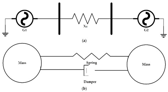
Figure 3.
(a) Power network model with no load. (b) Equivalent mass-spring-damper model of power network.
In this paper, a 60 Hz frequency is used in the simulation model. is the mechanical power (mechanical input from the turbine) and is the active power produced by a generator. The swing equation for synchronous machine for non-zero damping factor is presented in (23) and (24). Substituting the equations [19] for Definition 9, the swing equation for the generator in the power network is represented as:
It must be noted that the power generation units (generators) are not always directly connected to the power grid as presented in the simple mass-spring-damper model. The connectivity of generators is achieved via buses. The ordinary differential equation model of the swing equation does not truly present the power system architecture. To model power system, Differential-Algebraic Equations are used [23]. It is assumed that the transmission lines are lossless and there is no external load in the power system. Loads are presented by using synchronous machines as a motor in the connected network topology.
Let the complex phasor voltage for generator and bus is defined as [24].
and = . The dynamics of the generator are then presented as [23]:
substituting the graph Laplacian for a power network based on Kirchhoff’s law, the following real and imaginary parts of generator dynamics are obtained.
Using the Kron reduction technique [25] the Kron reduced model for the above generator dynamics is presented below.
where .
The equation has similarity to the swing equation, but the Kron reduction technique’s important properties is that it may change the original network structure, implying that the generators are required to be directly connected [24].
In a microgrid, the main role of energy conversion is performed using power inverters. The modeling of the power inverter is, therefore, an important part of the power microgrid model. Let us assume that PV solar power generation is used as a power source in the microgrid. The interface of the power inverter in such a case will perform DC/AC conversion. Assuming that the DC voltage is presented as and the current as Assuming that the conversion is denoted as and , respectively. Let represents the switching duty cycle of the inverter switches. let presents the switch-on of power inverter switching and presents the switch-off duration of inverter. The duty cycle in general will be represented as . Based on the above assumptions, the and is presented in (30).
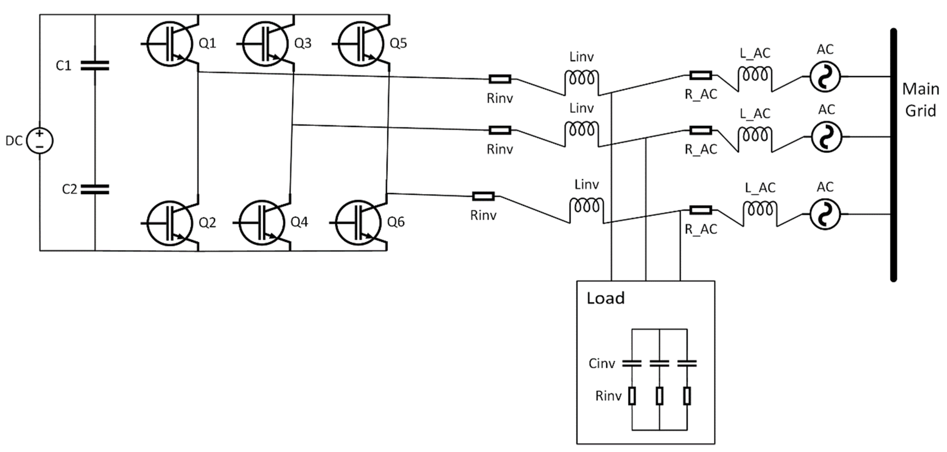
Let and present the switching frequency and magnitude of the power network, respectively. The power inverter interface shown in Figure 4 [19] is modeled in Equation (31).

Figure 4.
Basic three phase converter interface with DG.
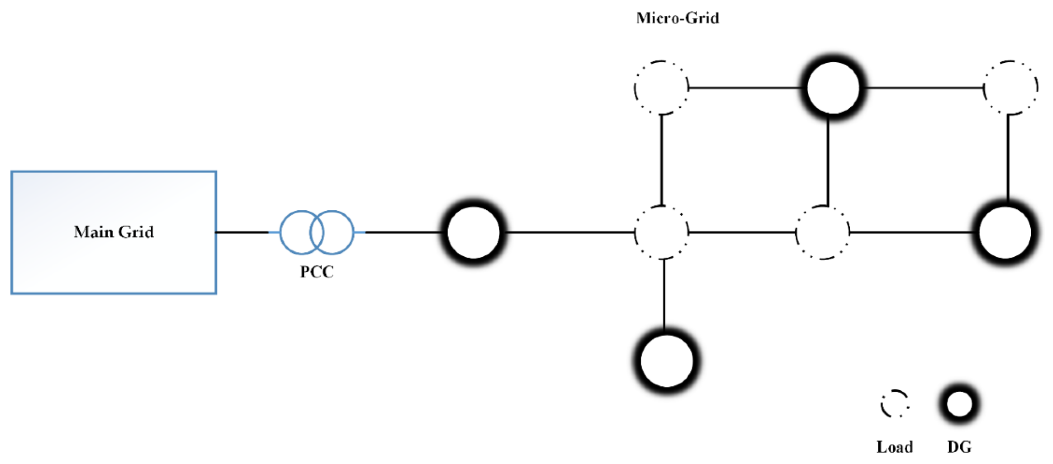
Similarly, the mathematical model may be developed with wind energy as a DG unit. The mathematical model of a microgrid connected to a power system via a point of common coupling is shown in Figure 5. The model is developed with as setpoints for active and reactive power injection, as the grid measurements (current, voltage, power, angle and frequency deviations) and as a load demand on all the bus power system buses. The steady-state model of the power network at the bus (based on Kirchhoff’s laws) is presented below [23].
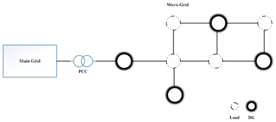
Figure 5.
Basic microgrid model.
The model developed in Equation (32) is referred as a physical model. The cyber model for Equation (32) is based on the input signal (physical model parameters) and output function (information of power grid). Defining the bus voltage , angles , active and reactive power (), the DG and load buses in the power system must satisfy Kirchhoff’s laws. The above dynamic model of a power network has a set of applications in the efficiency and stability analysis of power systems.
4. Inverter Interface Microgrid Components and Control Strategies Review
4.1. Modeling of Microgrid
This section covers the AC microgrid modeling using the power inverter interface. The microgrid in the power system comprises of power generation units, storage elements and load. In the power systems, the microgrid is interfaced through power inverters. As compared to synchronous generators, the frequency and voltage of the power microgrid are controlled at the inverter interface. A graph-theoretic approach is used to model the inverter interfaced microgrid. The inverter interfaced microgrid modeling mainly depends on the inverter operation model with reference to power lines, transformers, and loads. The main component of the power inverter is the power semiconductor switch (SCR, Thyristor, power BJT, Power FET, IGBT, IGCT). The power conversion from AC/AC and DC/AC depends on the switching ON/OFF of power electronic devices. The switching process is performed using modulation techniques such as Pulse Width Modulation (PWM) or Space Vector Pulse Width Modulation (SVPWM) [25]. The quality of the signal is improved (harmonics reduction) using a filter (LC). The design of the LC filter depends on the harmonics generated at the power inverter level. In power microgrids, there are two operational modes of inverters, the grid forming inverter and the grid-feeding inverter. The grid forming inverter controls the output voltage where different frequency and voltage control techniques are used to get the desired outcomes [26]. The grid-feeding inverters control the power microgrid’s active and reactive power connected to the network using different control schemes [27]. To understand the modeling of power microgrids, it is necessary to understand the modeling, behavior and control of the power inverter. The control of voltage sags/surges in the multi-agent-based model of the power microgrid network can be performed by the design of consensus controllers for voltage. The simplified consensus controllers to control voltage variations in the microgrid network at node i and node j is represented in Equation (31). The consensus controller for voltage variations in the microgrid networks may be used at the cyber layer in the microgrid network. The cyber layer provides the measurements in the network.
The control of voltage is referred as primary control that results in control of frequency deviations as well. The simplified consensus controller at node i and node j for power in microgrid networks is represented in Equation (32). The error calculations for Equations (33) and (34) are based on the information from the cyber layer. This error calculation helps in developing the distributed controllers to achieve consensus in voltage, frequency and power in power grid. The consensus in this case is the avoidance of voltage variation and frequency imbalance.
4.2. Modeling of Power Electronic Inverter
As discussed earlier, a microgrid comprises of a power inverter DG interface, load and storage elements. This section presents the modeling of a grid-forming inverter with fluctuating renewable DG with storage elements. The storage capacity has the advantage when power demands are increased. To model an inverter, an average switch modeling technique is used. This technique averages the internal inverter current and voltage over a switching period. For node , the three-phase voltage with phase angle is represented in Definition 7 as [17,18]:
Let presents the frequency, and present the continuously differentiable function and let be a non-negative constant. Let presents the clock drift of the processor used to operate the inverter. The closed-loop dynamics of the grid forming inverter are presented as:
In the hierarchy of power systems, is set by the higher level (primary level) control [26]. Let and , present the state signal, input and continuously differentiable function at higher-level control. is the output signal at this level required to be set for the secondary level control. The inverter higher-level control structure is presented as:
Substituting the above equation in the close loop dynamics of the grid forming inverter for the node are obtained as:
The grid-feeding inverters typically operate as current or power sources in the microgrid. The control design for the grid-feeding inverters is the same as grid forming inverters, but in the current scenario current or power references are employed. The reference signals are obtained using higher-level control. Let denote the state signal, port interconnection signal and continuously differentiable functions at node . Let denote the non-negative constant. The dynamic model of the grid-feeding inverter is presented as:
4.3. Modeling of Power Transmission Lines
This section discusses the power transmission lines also referred to as connectivity (edge set) in the context of graph theory. The three-phase symmetric RLC elements present all the power transmission lines. We assume that the power line is composed of constant ohmic resistance, constant inductance and constant capacitance in series at each phase. The voltage drops across the line is defined as . Let the state variable of the line be with the interconnection port variables and . The model of the line is presented as:
where represents the charge.
Let , and . Using the same assumption for nodal voltages and nodal currents as . The line voltage and current are presented as and respectively. The KCL and KVL relation using the graph theoretic analysis states and , where represents network connectivity [19]. The above transmission line model is presented as:
For simplicity, assume that all the power transmission lines and transformers are composed of symmetric three phase elements. The reduced symmetric model is presented as:
Let , rewriting the model equations in the form of state variables, the above model is simplified as below.
Using the graph theoretic representation of current and voltage for KCL and KVL the following mathematical model for power transmission lines is developed.
For some phase angle , the above model is transformed to dq coordinates using the Definition 5.
Using the above substitutions, the power transmission line model can be re-written as follows:
4.4. Modeling of Microgrid Protection System
The increased penetration of renewable energy resources and its effects on the power systems have encouraged the control community to develop an intelligent protection mechanism. The protection mechanism detects the faults in the power lines/buses. The detection of faults in the operation of microgrid and restoration is performed intelligently [28,29]. Let the protection system for the power inverters be denoted as , transmission lines as , DG unit as . The functions measure the fault levels at the respective sides and perform the protection operation e.g., In the transmission line operation, the short circuit currents are detected, and relay/circuit-breaker/auto-reclosing operation is performed. The protection mechanism is usually required to secure the microgrid/power grid components due to faults in the power system. The generalized mathematical function for microgrid protection is represented as:
4.5. Microgrid Model
Based on the modeling of grid forming, grid feeding and power transmission line, we can model the microgrid as a multi-agent model. Let and .
Combining the mathematical models of power inverters and transmission lines, the overall model of the microgrid is represented in
The above model of a power microgrid in Equation (46) may be utilized in the multi-agent-based control schemes for voltage (primary control) and active and reactive power control. The above microgrid model may also be utilized in the stability analysis of multi-agent-based microgrid systems. The above mathematical model addresses the stability and control challenges for complete system components. The stability analysis may include generation units, power inverters, transmission lines, protection devices and load. Thus, proving this mathematical model as a useful tool in adressing set of applications in the analysis of power systems protection, stability and control.
Modeling of Power Microgrid in Island Mode
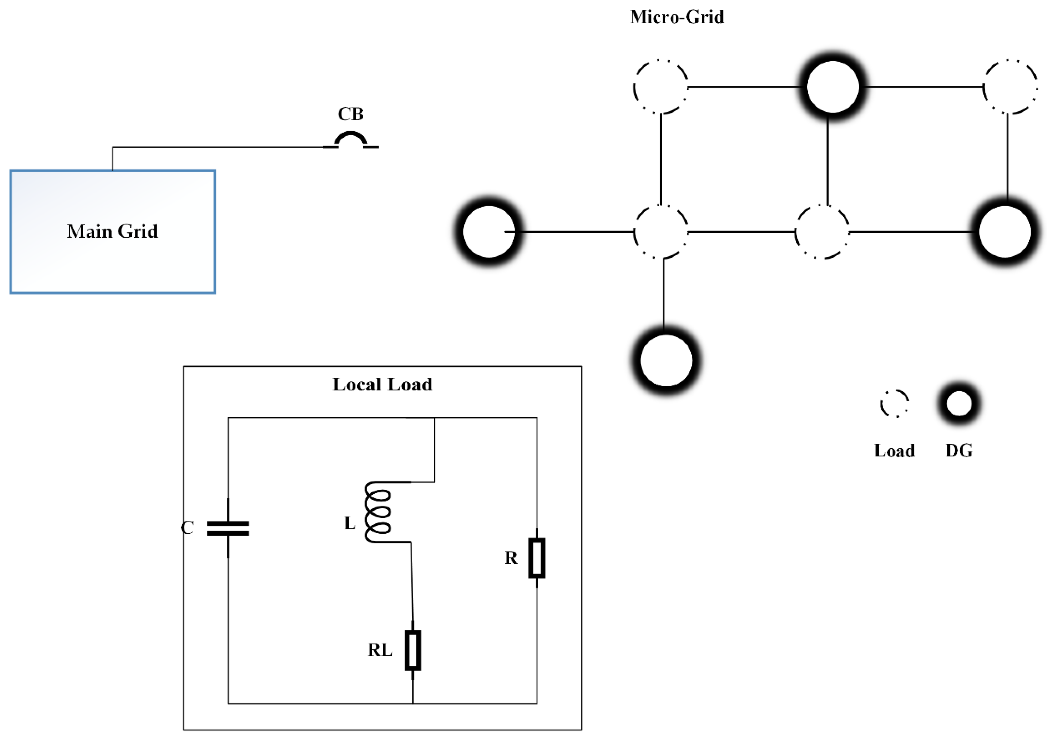
Consider the microgrid presented in Figure 6. The voltage and frequency control is managed by dual control layers, i.e., the centralized control of power microgrid and DG distributed/decentralized control. Various grid faults, such as low/high voltageride through in wind farms which causes the DG unit(s) to be disconnected from the main grid. Such a capability of a DG unit(s) is referred as the Island mode of DG unit/microgrid [7]. The control scheme for an Island mode microgrid is a challenging task and thus requires the modeling of microgrid connected with the local load. Consider the microgrid in Figure 5 [19] with the circuit breaker (CB) opened due to faults.
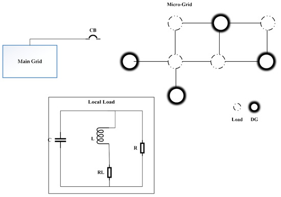
Figure 6.
Microgrid in Islanded mode.
We assume RLC loads in the microgrid as local loads and RLC transmission lines. The microgrid modeling is performed using abc-dq transformation. We assume that the DG unit is a DC source and the inverter operation is DC/AC. Let the voltage and current at the RL distribution level be represented as and . represent the load while is the resistance of distribution level. The voltage at the PCC is denoted as . The main grid voltage, inductance and resistance are represented as and . For an Islanded mode operation, the circuit breaker opens disconnecting the microgrid from the main grid. The mathematical modeling [12] of the system is represented below.
With reference to Definition 5 the above system could be transformed to dq reference frame as:
The state-space model of the above system is presented in general as:
where and are system, input and output matrices respectively and represents the state of the system, is the output and represents the control input.
Choosing the transformation frame in such a way that the quadrature component and its derivative is cancelled. This simplifies the equation further, as shown in Equation (51).
And
For DG units in the islanded microgrid, the above system will be formulated as:
where , , with and are matrices derived using system state, input and output.
The above model is valid for energy sources such as solar PV generation or wind power with an additional AC/DC inverter interface. Coupling the heterogeneous DG units with the main grid using a power electronic inverter interface offers challenges, such as voltage stability, phase stability, frequency stability, active and reactive power stability and fault ride-through capabilities.
4.6. Control Strategies for the Power Microgrid: Review
The control of power inverters in microgrid control plays a major role in the stability analysis of the power network. Power inverters play a major role in the integration of DGs in the power system. Various control algorithms have been developed for the power inverters to ensure reliability and efficiency in the power network. Power grid problems such as unbalanced power, harmonic distortions, voltage fluctuations and frequency deviations are the main concerns in the stability of the power network [26]. Power compensation for single-phase DG system through Model Predictive Control (MPC) compensated the reactive power in the network [30]. To minimize the active and reactive power oscillations in the power network, dual current control strategy is developed in [31]. To ensure voltage stability with minimum frequency deviations and flexible active and reactive power control, a robust grid synchronization scheme is developed [32]. Similarly, the droop control for frequency and voltage stability is developed in [33]. Hysteresis control and robust adaptive control for power inverter interfaced microgrid for grid mode and islanded mode is discussed in [34].
5. Challenges and Opportunities in the Power Systems’ Stability and Control
The penetration of renewable energy resources renders a sustainable power system. Wind power and solar energy generation deployment is rapidly increasing in the power systems replacing conventional power generation units. The increased penetration from remote areas is giving rise to the concept of the microgrid, resulting in control and stability challenges in energy storage, transmission lines and distributed systems [35].
5.1. Challenges in Energy Storage Units
Energy storage capability in the power network is advantageous in the case of increased energy demand. Energy storage reduces generation reserve requirements and maximizes the use of variable generation units. In contrast to those advantages, the energy storage units require power conversion mechanisms (DC/AC). The power conversion mechanism may result in power loss [36]. The major disadvantage of an energy storage unit is the cost price of each unit. Different storage energy scheduling algorithms and optimization algorithms have been developed in this regard. A comprehensive cost to benefit ratio study is required in the use of energy storage capability in power systems with variable energy generation units as well as in electric vehicle usage in case of the vehicle-to-grid and the grid-to-vehicle scenario.
5.2. Challenges in Transmission and Distribution Systems
The environmental hazards of conventional power plants have encouraged renewable energy generation. With the increased demand in the power systems, distributed energy resource penetration resulting in microgrids has increased. Stable and efficient microgrid interconnection to the power network coordinated transmission and distribution system is required. The HVAC and HVDC transmission technologies are mainly used in the power networks for wide-area power transmission [36,37]. Trends in future transmission models depend on robustness in uncertainties such as voltage and frequency oscillations in the generation technology. Fundamental challenges in the transmission systems include renewable energy integration, design, and high-temperature low-sag conductors for ultrahigh transmission and cost optimization.
5.3. Challenges in Distributed Control
The control scheme is mainly based on local measurements with guidance from centralized control. It manages the local power balancing issues as well as ensures the stability of the local power system with no effects on the large, interconnected power network. The use of power-inverter interfaced energy generation units (renewable resources and residential units) makes dynamic stability analysis of power network very complex. Frequency and voltage stability control are challenging tasks in the grid-connected mode and island mode [26]. Conventional control schemes have limitations in such scenarios. The need for reformulated real-time control design is required for the power network’s dynamic stability analysis. Reformulation of conventional control and development of new regulatory reforms in the power network is required.
Centralized control operation ensures the efficiency, stability and reliability of the large power network. The future centralized power grid control will be more challenging due to the increasing autonomy of distributed control schemes at the local level. Centralized control of the power grid ensures the stability and synchronization of power throughout the network. Future challenges of the centralized power grid include monitoring all units, predicting potential issues, and countermeasures to avoid those issues.
The challenges in the power inverter interface and control, stability of power microgrid with reference to voltage, frequency and power, transmission lines and protection mechanism may all be addressed using the mathematical models developed in Equations (48) and (52) for main grid and microgrid networks and islanded microgrids, respectively.
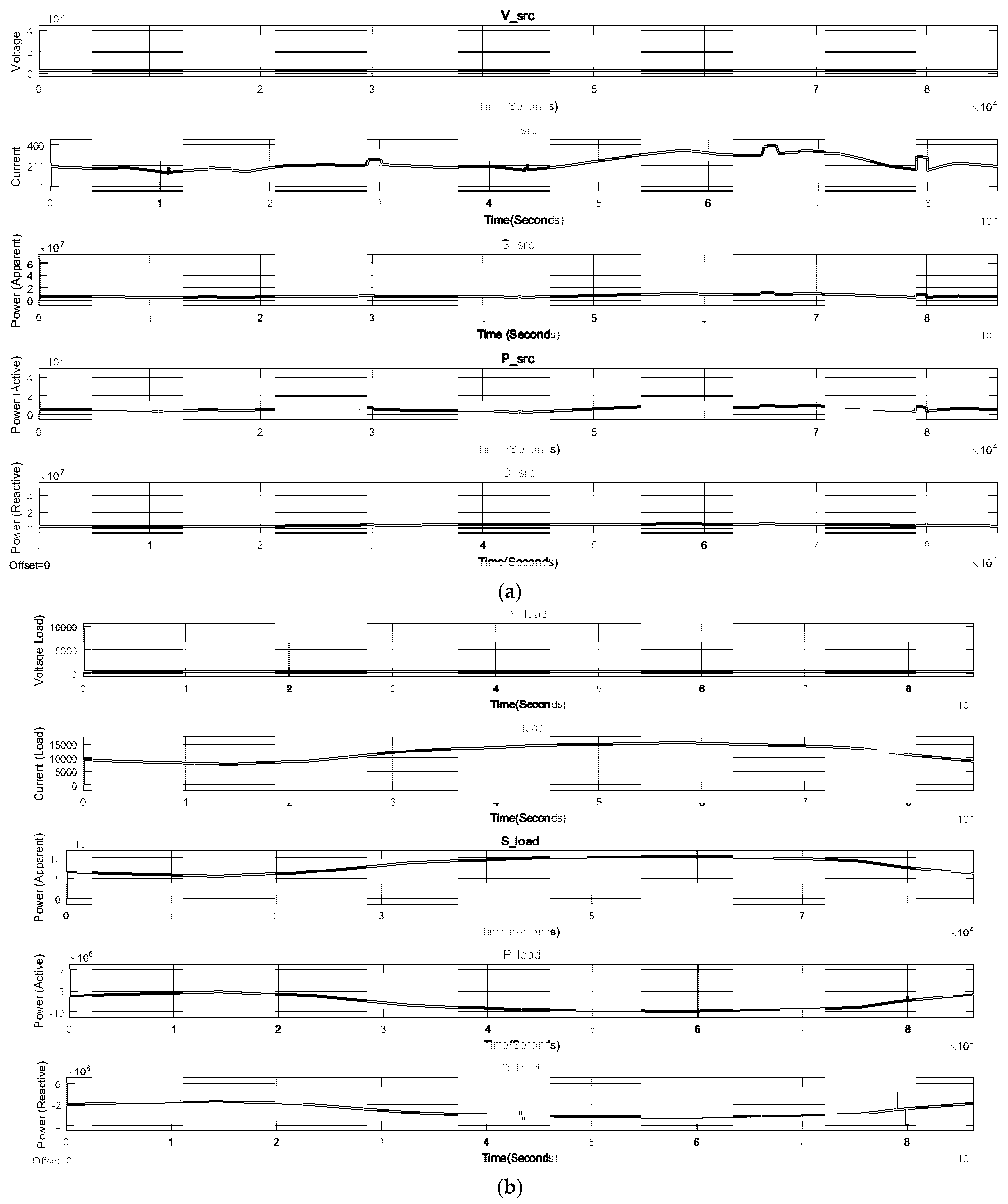
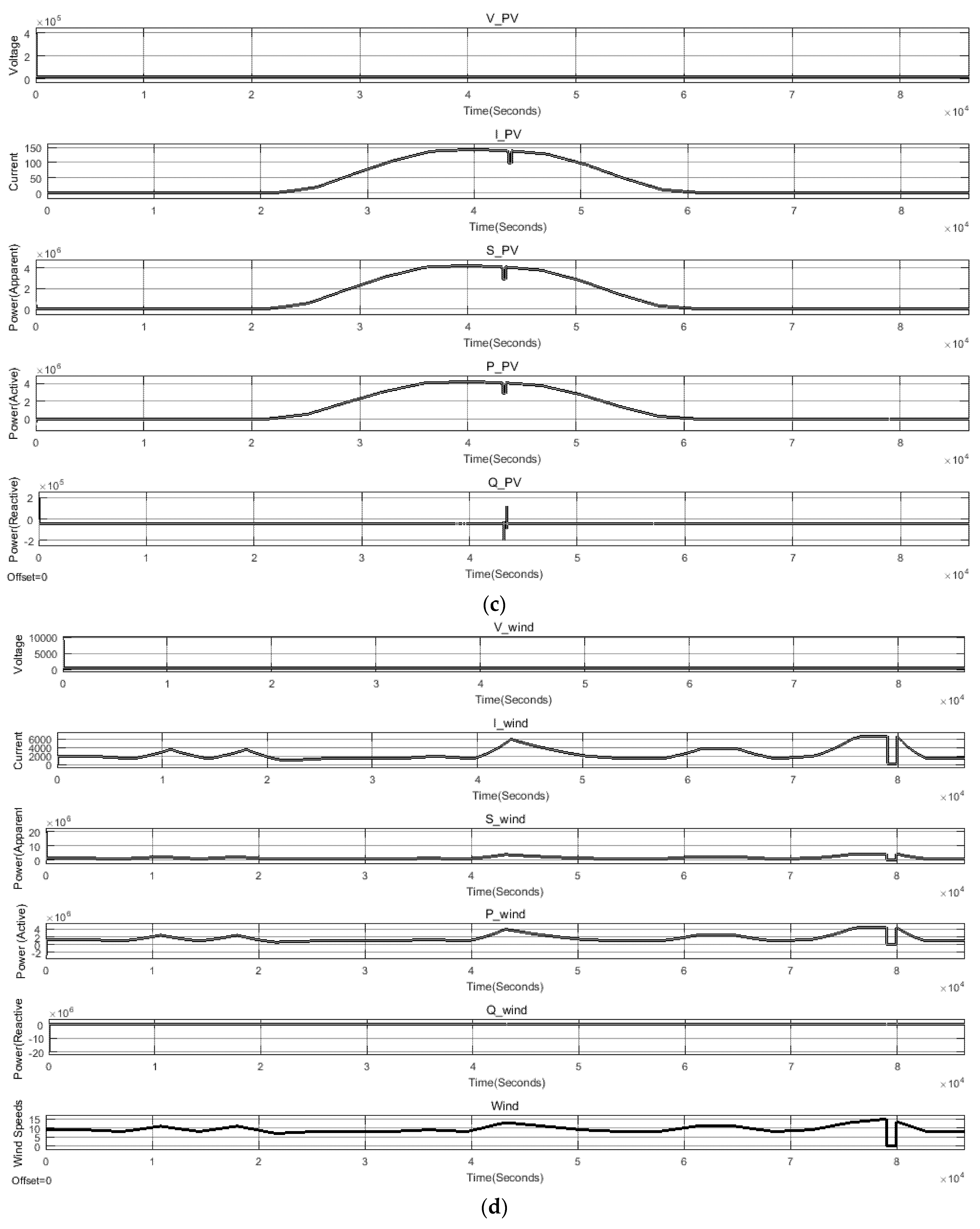
A standard microgrid model featuring a multi-agent system approach is developed, as shown in Figure 7. The physical model for the multi-agent-based network model is presented in Figure 6. The cyber layer measures the network parameters such as voltage, power and frequency. Using the cyber layer, the system variations may be measured and errors may be reduced by using consensus based controllers. The analysis of the total grid generation, wind power generation, solar PV generation and load of designed main grid is presented in Table 1. The system is connected via a 25 kV transmission line/bus to the main grid. The transmission line may be of 11 kV, 6 kV, 3.3 kV as well based on the distribution line ratings. A step-down transformer of 0.6 kV is used to distribute the power to the consumer/load. The system operates at 60 Hz frequency. The total power generated (real, reactive and apparent), current, voltage and load for the main grid model are presented in Figure 8a–f below.

Figure 7.
Multi-agent-based microgrid model.

Table 1.
Main grid and microgrid analysis.
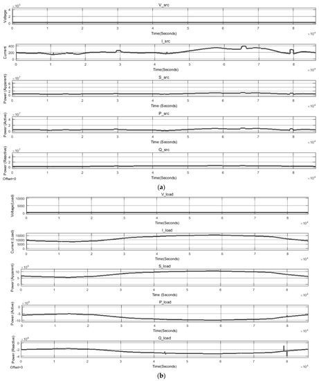
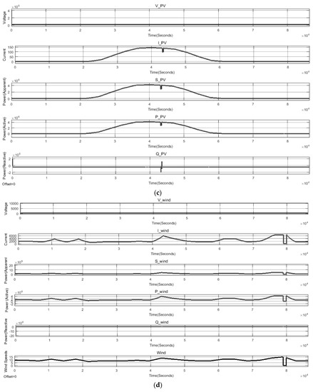
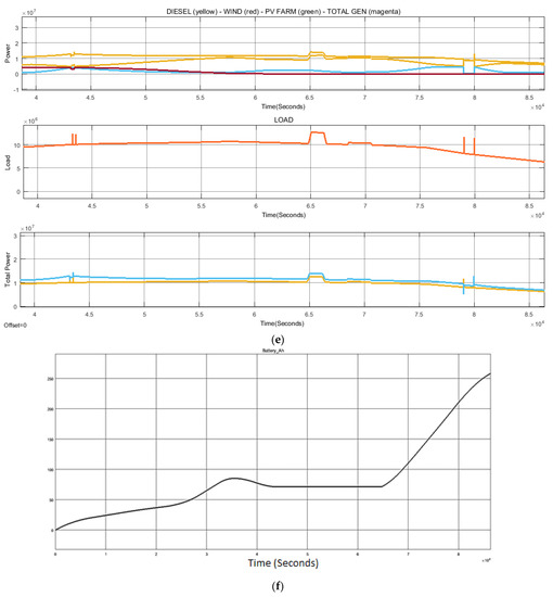
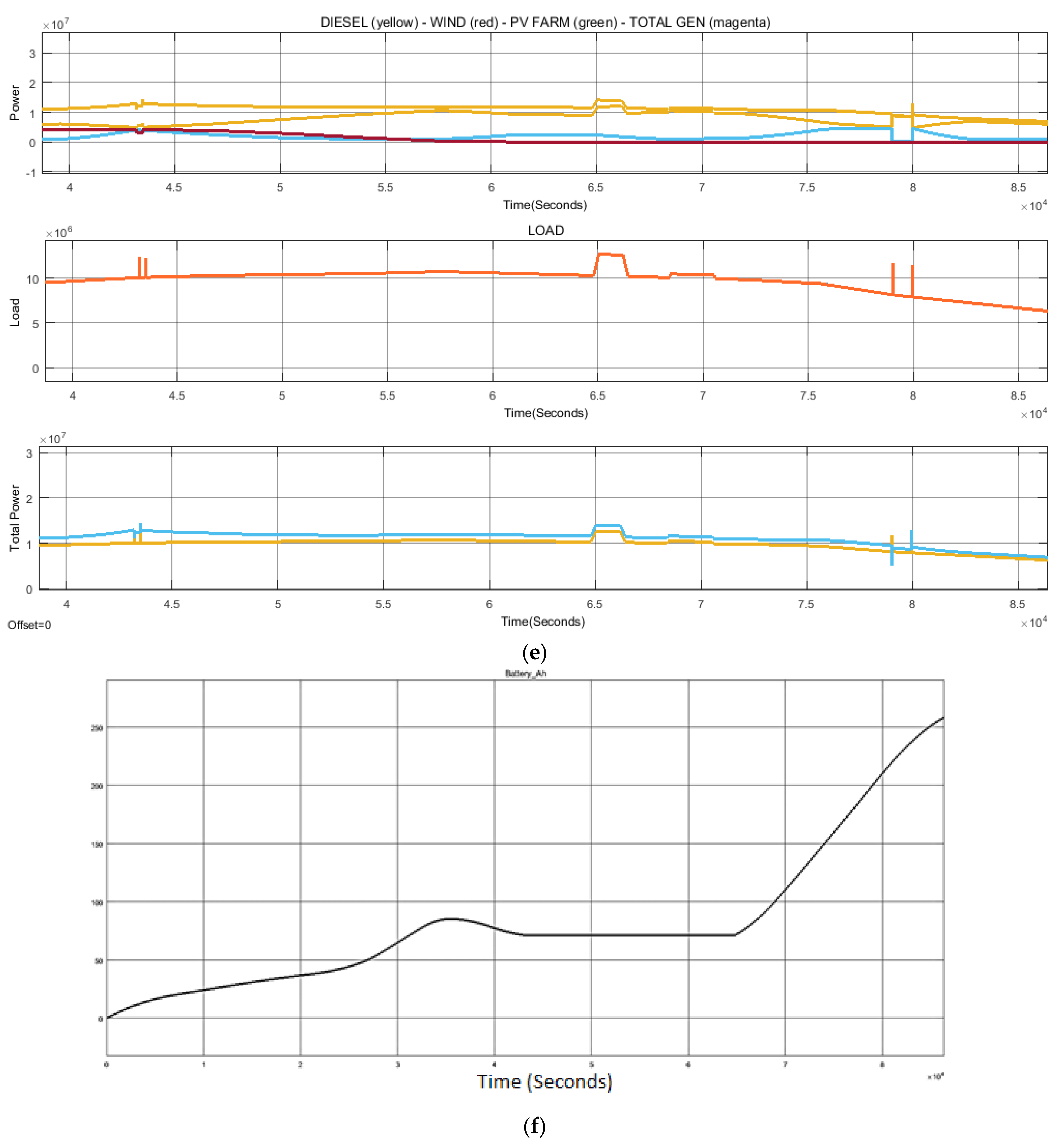
Figure 8.
(a) Analysis of generation source in main grid. (b) Load analysis for main grid. (c) Solar PV analysis in main grid. (d) Wind farm analysis in main grid. (e) Total power analysis in main grid. (f) Battery capacity in Ampere-hours.
The load flow of the simulated system is presented in Table 2. The load flow presents base voltage (bus voltage) also referred as transmission line voltage, reference voltage (pu), generation sources of main grid and microgrid as well as load.
Table 2.
Load flow of simulated model.
The line parameters (RLC line parameters) are presented in the form of matrices as discussed in Section 2. The ground resistivity for the modeled system is taken as 100 ohms. The resistance matrix (ohm/km) is presented as , The inductance matrix (H/km) is presented as and the capacitance matrix (F/km) is presented as . The computed values used in the simulation based on the reference voltage, base voltage, line voltage and generation sources are presented below as:
Based on the above line parameters, the system is modeled using the configuration presented in Figure 6. Node i and node j represent the microgrids comprising of renewable as well as conventional energy sources. The generation sources are presented as and the load is presented as .
The generation in the main grid representing voltage, current and power for the modeled system is presented in Figure 8a. The graph variations are due to variations in wind speed, solar irradiance as well as load demand.
The load analysis based on the generation sources in the main grid and microgrid is presented in Figure 8b. It is observed that the variation in reactive power (spikes) due to load variations as well as variation in renewable energy generation sources (wind, solar).
The analysis of solar PV generation is presented in Figure 8c. Solar irradiance of at degree with partial shading presenting a cloudy scenario is also considered for the modeled system. The spike in the system is observed due to an abrupt increase in load demand.
The wind farm is modeled with the nominal wind speeds at with cut-out speed at 21 m/s and cut-in speed of 3.5 m/s. The variation in wind power generation occurs due to variations in wind speeds as well as an increase in load demand.
The variations in wind speed, as well as the increase in load demand, result in reactive power and voltage control challenges. To address the challenges, power inverters along with LC filters are designed. In this case grid forming and grid-feeding inverters. The analysis of wind farms based on wind speeds is presented in Figure 8d.
The total power generated in the main grid as well as load consumption and sum for the microgrid is presented in Figure 8e.
A single storage unit (battery) of 250 Ampere hour rating is used. The state of charge of the battery is presented in Figure 8f.
6. Conclusions
In this paper, a detailed procedure to model a microgrid is presented with a graph-theoretic concept. A microgrid model is developed using fundamental electrical engineering and circuit analysis concepts. Basic definitions and mathematical representation are discussed as fundamental literature for the modeling of the microgrid. A synchronous machine mathematical model is used for the modeling of the power system. General circuit theory is used to model transmission lines, load and generation units. A multi-agent-based microgrid model using graph-theoretic concepts is used in power network modeling. The results are presented in the end with renewable energy penetration for the main grid model and microgrid model. The mathematically modeled system motivates the cyber-physical modeling and control of the power system. The developed model highlights the complex interation challenges between the cyber and physical system. The model addresses issues such as power system performance, frequency imbalance, voltage variations and change in load. It opens a paradigm to apply cyber security to large-scale power networks as cyber-physical systems. This paradigm shift will address the challenges such as power quality, frequency detrioration, voltage regulation, energy management effeciently. The developed model may be utilized in cyber attack detection and mitigation control schemes for power networks.
Author Contributions
Conceptualization, A.H. and S.T.H.R.; methodology, A.H; software, A.H. and M.U.S.; validation, A.H. and S.T.H.R.; formal analysis, A.H.; investigation, A.H.; resources, H.A.; data curation, A.H.; writing—original draft preparation, A.H. and S.T.H.R.; writing—review and editing, A.H. and H.A.; visualization, M.U.S.; supervision, S.T.H.R.; project administration, A.H.; funding acquisition, All authors have read and agreed to the published version of the manuscript.
Funding
This research received no external funding.
Institutional Review Board Statement
Not Applicable.
Informed Consent Statement
Not Applicable.
Data Availability Statement
Not Applicable.
Conflicts of Interest
The authors declare no conflict of interest.
References
- Tamimi, B.; Canizares, C.; Bhattacharya, K. System Stability Impact of Large-Scale and Distributed Solar Photovoltaic Generation: The Case of Ontario, Canada. IEEE Trans. Sustain. Energy 2013, 4, 680–688. [Google Scholar] [CrossRef]
- Serag ElDin, A.M.A.M.; El-Mahgary, Y.; Ali, A.H.H.; Khairy, A. Comparing socioeconomic & environmental impacts of building 2GW PV power plant in both sides of the Medeterranian. In Proceedings of the 2013 International Renewable and Sustainable Energy Conference (IRSEC), Quarzazate, Morocco, 7–9 March 2013; pp. 331–336. [Google Scholar]
- Blaabjerg, F.; Teodorescu, R.; Liserre, M.; Timbus, A.V. Overview of Control and Grid Synchronization for Distributed Power Generation Systems. IEEE Trans. Ind. Electron. 2006, 53, 1398–1409. [Google Scholar] [CrossRef] [Green Version]
- Cao, Y.; Wang, X.; Li, Y.J.; Tan, Y.; Xing, J.; Fan, R. A comprehensive study on low-carbon impact of distributed generations on regional power grids: A case of Jiangxi provincial power grid in China. Renew. Sustain. Energy Rev. 2016, 53, 766–778. [Google Scholar] [CrossRef]
- Natesan, C.; Ajithan, S.K.; Palani, P.; Kandhasamy, P. Survey on Microgrid: Power Quality Improvement Techniques. ISRN Renew. Energy 2014, 2014, 342019. [Google Scholar] [CrossRef]
- Sen, S.; Kumar, V. Microgrid control: A comprehensive survey. Annu. Rev. Control 2018, 45, 118–151. [Google Scholar] [CrossRef]
- Nikos, D. Hatziargyriou Microgrids: Architectures and Control; Hatziargyriou, N., Ed.; Wiley-IEEE Press: Athens, Greece, 2013; ISBN 978-1-118-72064-6. [Google Scholar]
- Dorfler, F.; Bolognani, S.; Simpson-Porco, J.W.; Grammatico, S. Distributed Control and Optimization for Autonomous Power Grids. In Proceedings of the 2019 18th European Control Conference (ECC), Naples, Italy, 25–28 June 2019; pp. 2436–2453. [Google Scholar]
- Invernizzi, G.; Vielmini, G. Challenges in Microgrid Control Systems Design. An application case. In Proceedings of the 2018 AEIT International Annual Conference, Bari, Italy, 3–5 October 2018; pp. 1–6. [Google Scholar]
- Nejabatkhah, F.; Li, Y.W.; Tian, H. Power Quality Control of Smart Hybrid AC/DC Microgrids: An Overview. IEEE Access 2019, 7, 52295–52318. [Google Scholar] [CrossRef]
- Mahmoud, M.S. Microgrid Control Problems and Related Issues. In Microgrid; Elsevier: Dhahran, Saudi Arabia, 2017; pp. 1–42. [Google Scholar]
- Zeng, Z.; Yang, H.; Zhao, R. Study on small signal stability of microgrids: A review and a new approach. Renew. Sustain. Energy Rev. 2011, 15, 4818–4828. [Google Scholar] [CrossRef]
- Majumder, R. Some Aspects of Stability in Microgrids. IEEE Trans. Power Syst. 2013, 28, 3243–3252. [Google Scholar] [CrossRef]
- Elrayyah, A.; Sozer, Y.; Elbuluk, M. Simplified modeling procedure for inverter-based islanded microgrid. In Proceedings of the 2012 IEEE Energytech, Cleveland, OH, USA, 29–31 May 2012; pp. 1–6. [Google Scholar]
- Patowary, M.; Panda, G.; Deka, B.C. Reliability Modeling of Microgrid System Using Hybrid Methods in Hot Standby Mode. IEEE Syst. J. 2019, 13, 3111–3119. [Google Scholar] [CrossRef]
- Kundur, P.; Balu, N.J.; Lauby Mark, G. Power System Stability and Control; McGraw-Hill: New York, NY, USA, 1994. [Google Scholar]
- Bahrami, S.; Mohammadi, A. Smart Microgrids, Bahrami, S., Mohammadi, A., Eds.; Springer International Publishing: Cham, Switzerland, 2019; ISBN 978-3-030-02655-4. [Google Scholar]
- Vittal, V.; McCalley, J.D.; Anderson, P.M.; Fouad, A.A. Power System Control and Stability, 3rd ed.; Wiley-IEEE Press: Hoboken, NJ, USA, 2019; ISBN 978-1-119-43371-2. [Google Scholar]
- Ishizaki, T.; Chakrabortty, A.; Imura, J.-I. Graph-Theoretic Analysis of Power Systems. Proc. IEEE 2018, 106, 931–952. [Google Scholar] [CrossRef]
- Godsil, C.; Royle, G. Algebraic Graph Theory (Graduate Texts in Mathematics); Springer: New York, NY, USA, 2001; Volume 207, ISBN 978-0-387-95220-8. [Google Scholar]
- Zamora, R.; Srivastava, A.K. Controls for microgrids with storage: Review, challenges, and research needs. Renew. Sustain. Energy Rev. 2010, 14, 2009–2018. [Google Scholar] [CrossRef]
- Hasan, N.S.; Hassan, M.Y.; Majid, M.S.; Rahman, H.A. Review of storage schemes for wind energy systems. Renew. Sustain. Energy Rev. 2013, 21, 237–247. [Google Scholar] [CrossRef]
- Dorfler, F.; Simpson-Porco, J.W.; Bullo, F. Electrical Networks and Algebraic Graph Theory: Models, Properties, and Applications. Proc. IEEE 2018, 106, 977–1005. [Google Scholar] [CrossRef]
- Dorfler, F.; Bullo, F. Kron Reduction of Graphs With Applications to Electrical Networks. IEEE Trans. Circuits Syst. I Regul. Pap. 2013, 60, 150–163. [Google Scholar] [CrossRef] [Green Version]
- Schiffer, J.; Ortega, R.; Astolfi, A.; Raisch, J.; Sezi, T. Conditions for stability of droop-controlled inverter-based microgrids. Automatica 2014, 50, 2457–2469. [Google Scholar] [CrossRef] [Green Version]
- Khayat, Y.; Shafiee, Q.; Heydari, R.; Naderi, M.; Dragicevic, T.; Simpson-Porco, J.W.; Dorfler, F.; Fathi, M.; Blaabjerg, F.; Guerrero, J.M.; et al. On the Secondary Control Architectures of AC Microgrids: An Overview. IEEE Trans. Power Electron. 2020, 35, 6482–6500. [Google Scholar] [CrossRef]
- Morsali, J.; Zare, K.; Tarafdar Hagh, M. Applying fractional order PID to design TCSC-based damping controller in coordination with automatic generation control of interconnected multi-source power system. Eng. Sci. Technol. Int. J. 2017, 20, 1–17. [Google Scholar] [CrossRef] [Green Version]
- Liu, Z.; Su, C.; Hoidalen, H.K.; Chen, Z. A Multiagent System-Based Protection and Control Scheme for Distribution System With Distributed-Generation Integration. IEEE Trans. Power Deliv. 2017, 32, 536–545. [Google Scholar] [CrossRef]
- Kiel, E.S.; Hovin Kjolle, G. The impact of protection system failures and weather exposure on power system reliability. In Proceedings of the 2019 IEEE International Conference on Environment and Electrical Engineering and 2019 IEEE Industrial and Commercial Power Systems Europe (EEEIC / I&CPS Europe), Genova, Italy, 10–14 June 2019; pp. 1–6. [Google Scholar]
- Hu, J.; Zhu, J.; Dorrell, D.G. Model predictive control of inverters for both islanded and grid-connected operations in renewable power generations. Iet Renew. Power Gener. 2014, 8, 240–248. [Google Scholar] [CrossRef] [Green Version]
- Hojabri, M.; Ahmad, A.Z.; Toudeshki, A. An Overview on Current Control Techniques for Grid Connected Renewable Energy Systems. Int. Proc. Comput. Sci. Inf. Technol. 2012, 56, 119. [Google Scholar]
- Rodriguez, P.; Luna, A.; Candela, I.; Mujal, R.; Teodorescu, R.; Blaabjerg, F. Multiresonant Frequency-Locked Loop for Grid Synchronization of Power Converters Under Distorted Grid Conditions. IEEE Trans. Ind. Electron. 2011, 58, 127–138. [Google Scholar] [CrossRef] [Green Version]
- Tayab, U.B.; Roslan, M.A.B.; Hwai, L.J.; Kashif, M. A review of droop control techniques for microgrid. Renew. Sustain. Energy Rev. 2017, 76, 717–727. [Google Scholar] [CrossRef]
- Arfeen, Z.A.; Khairuddin, A.B.; Larik, R.M.; Saeed, M.S. Control of distributed generation systems for microgrid applications: A techno-logical review. Int. Trans. Electr. Energy Syst. 2019, 29, e12072. [Google Scholar] [CrossRef] [Green Version]
- Yoo, H.-J.; Nguyen, T.-T.; Kim, H.-M. Consensus-Based Distributed Coordination Control of Hybrid AC/DC Microgrids. IEEE Trans. Sustain. Energy 2020, 11, 629–639. [Google Scholar] [CrossRef]
- Hossain, E.; Hossain, J.; Un-Noor, F. Utility Grid: Present Challenges and Their Potential Solutions. IEEE Access 2018, 6, 60294–60317. [Google Scholar] [CrossRef]
- Telukunta, V.; Pradhan, J.; Agrawal, A.; Singh, M.; Srivani, S.G. Protection challenges under bulk penetration of renewable energy resources in power systems: A review. CSEE J. Power Energy Syst. 2017, 3, 365–379. [Google Scholar] [CrossRef]

Publisher’s Note: MDPI stays neutral with regard to jurisdictional claims in published maps and institutional affiliations. |
© 2022 by the authors. Licensee MDPI, Basel, Switzerland. This article is an open access article distributed under the terms and conditions of the Creative Commons Attribution (CC BY) license (https://creativecommons.org/licenses/by/4.0/).