Modeling Lane-Changing Behavior Based on a Joint Neural Network

Abstract

This paper proposes a joint neural network model to imitate lane-changing behaviors. Specifically, lane-changing decision-making process is captured by probabilistic neural network (PNN) and lane-changing decision-making process is learned by back-propagation neural network (BPNN). The link between the two neural networks is the target gap for lane-changing. After testing and calibrating the joint neural network model, simulation experiments are designed to study heterogeneous traffic flow at an off-ramp bottleneck. Numerical simulations are conducted in various traffic scenarios with different market penetration rates (MPRs) of intelligent vehicles (IVs) and proportions of exit vehicles. Finally, the performance of heterogeneous flows is evaluated from the perspectives of average speed, road capacity, and safety. The results show that joint neural network can accurately predict the gap types chosen for lane changes and vehicle trajectory during lane-changing. For the traffic system, road capacity obtains the least value when the MPR of IVs is 50%. Moreover, frequent lane-changing movements upstream the off-ramp bottleneck determine the areas at greatest risk. However, when MPR of IVs is over 80% or proportion of exit vehicles is below 15%, both traffic efficiency and safety can be significantly improved. This work provides some insights into the application of machine learning algorithms to traffic flow modeling, and conducts quantitative analysis on the impact of key parameters on traffic systems. Findings of this work can support management and operation of automated highway systems in the future.

1. Introduction

The field of intelligent vehicles (IVs) is rapidly growing worldwide from intelligent control systems to intelligent sensors. These systems or sensors offer the potential for considerable enhancements in traffic efficiency and safety. Meanwhile, intelligent vehicular technologies are gradually changing the movements of decision-making and execution process. Especially, vehicle-to-everything (V2X) communications can transform valid information to surrounding vehicles or the roadside unit. It helps drivers prevent road collisions and avoid dangerous situations by sharing data with other vehicles [1,2]. In this case, IVs can gain sufficient information in a connected environment to operate efficiently and safely. For example, potential benefits include making an optimal decision on the target gap for lane-changing, and executing a set of high-quality movements with a wiser central controller. Generally, two main control subjects are longitudinal and lateral movements of vehicles in the traffic stream [3,4].

For the longitudinal control, there are a lot of classic models designed to simulate car-following behaviors. Particularly, the intelligent driver model (IDM) introduced by Kesting et al. [5] has been proposed to imitate longitudinal dynamics of manually driven vehicles (MVs). For IVs, adaptive cruise control (ACC) system is developed to assist drivers and improve driving safety. In the previous theoretical research, simulations have been extensively conducted to demonstrate the efficiency and stability of ACC systems. As an enhanced version of ACC, cooperative ACC (CACC) forms the basis of connected and autonomous vehicles, which can notably smooth hazardous traffic flow [6,7,8,9,10,11]. In this paper, both ACC vehicles and CACC vehicles are collectively referred to IVs.

Moreover, the mixed traffic flow with MVs and IVs is investigated and the transportation system is evaluated by several indexes in different aspects of performance. Ye and Arvin et al. explored the impact of connected and autonomous vehicles (CAVs) on traffic safety respectively in freeway and intersection scenarios [12,13,14]. Zhou et al. estimated the effect of CAV platoon and CACC market penetration rate on fuel consumption and emissions based on IDM and ACC/CACC models [7]. Wang et al. presented a framework for the analytical study on stability of CACC-manual heterogeneous vehicular flow with partial CACC performance degrading [15]. Additionally, Mahdinia et al. evaluated the safety, energy, and emissions impacts of automated and cooperative systems in mixed traffic containing conventional, ACC and CACC vehicles [16]. Results of the above-mentioned literature indicate that the implementation of IVs would be beneficial for better traffic.

Compared with longitudinal control models in a commercial application, research on lateral control has not formed unified criteria or frameworks due to complexity and confidentiality in lane-changings. Gipps proposed a structure of lane-changing decisions, which was applied for the urban situation [17]. Following Gipps’s pioneering work, many researchers have been devoted to the extension or improvement of the model [2,18]. For example, Kesting et al. introduced a general model (minimizing overall braking induced by lane change, MOBIL) to derive lane-changing rules for discretionary and mandatory lane changes [19]. Toledo et al. presented a generalized lane-changing model that explicitly incorporates the choice of target lane on the basis of the utilities of current and adjacent lanes [20].

With the rapid development of IVs, studies are being conducted on modeling or predicting intelligent vehicles’ lane-changing movements, including CAVs and automated vehicles (AVs). Ye and Yamamoto modeled CAVs’ car-following and lane-changing maneuvers in heterogeneous traffic flow based on cellular automaton [12,13]. Shamir designed a smooth and ergonomic optimal lane-change trajectory for an AV’s three-phase overtaking maneuver [21]. Yang et al. proposed a dynamic lane-changing trajectory planning model for AVs. Lane-changing could be finished smoothly, efficiently, and safely controlled by this new model [22]. Besides, research on lane-changing of IVs can be related to control methods, such as ramp metering and variable speed limit.

Moreover, many lane-changing behaviors cannot be precisely represented by the conventional rule-based models. Therefore, more and more data-driven models are proposed to imitate lane-changing [23,24,25,26]. Mahajan et al. presented an end-to-end machine learning model for predicting lane-change maneuvers from unlabeled data based on support vector machine (SVM) and long short-term memory (LSTM) [24]. Das et al. modeled lane-change behavior for AVs using a supervised machine learning approach and compared different machine-learning-based classifiers [25]. Xie et al. used deep belief network and LSTM neural network to model the lane-changing decision-making and implementation processes [26]. The above-mentioned models for lane-changing take into account many factors and capture more accurate features. Generally, this kind of modeling method has a great application prospect in accident prevention and efficiency improvement.

Although a number of studies have been dedicated to lane-changing modeling and future traffic flow prediction, there has not been any joint neural networks for IVs or CAVs in terms of lane-changing behavior learning. Moreover, with respect to off-ramp bottlenecks, research were not as sufficient as the scenarios of on-ramp and basic section on freeways. Off-ramp is a more complex scenario, and has significant impact on travel efficiency and safety. So, it needs more exploration in traffic state prediction and traffic system evaluation, especially for CAV environment in the future.

Therefore, this paper focuses on the following two issues: (1) models for lane-changing decision-making and execution behaviors, and (2) analysis of mixed traffic at an off-ramp bottleneck. Accordingly, the major contributions of this paper are summarized at two levels: (1) At the micro-level, the whole lane-changing process is divided into two stages and each stage is modeled by different neural network algorithms. Specifically, lane-changing decision-making model is based on probabilistic neural network (PNN) and lane-changing decision-making process is learned by BPNN. Then, calibration and testing experiments are conducted to prove the validation of the proposed joint neural network. (2) At the macro-level, the transportation system with human-driving and IVs is analyzed in terms of efficiency and safety. Moreover, two sensitive variables of the mixed traffic flow near an off-ramp, penetration rate of CACC vehicles and proportion of exit vehicles, are examined to achieve optimal performance. Findings of this study contribute to providing guidance on both theoretical research and potential practical applications.

The remainder of this paper is structured as follows. Methodology of this study is summarized in Section 2, Section 3 and Section 4. Specifically, Section 2 describes the simulation testbed, including car-following model, lane-changing model, and efficiency and safety evaluation models. Section 3 presents the results of calibration and testing for the proposed lane-changing model. Simulated traffic and scenario settings are introduced in Section 4. Numerical simulation results for evaluating the transportation system and analyzing sensitive variables are summarized in Section 5. Finally, this work is concluded with conclusions in Section 6.

2. Model Descriptions

This section presents the car-following and lane-changing models applied to simulate vehicles’ behavior in this study. Among them, the IDM and two typical ACC/CACC models are chosen to imitate the longitudinal control systems for MVs and IVs, respectively [5,9,10]. For lateral control, two typical neural network algorithms—PNN and BPNN—are chosen to imitate lane-changing behaviors. Finally, evaluation indexes of travel efficiency and safety are introduced for the following experiments.

2.1. Car-Following Model

(1)

MV: The IDM is accepted widely in the field of traffic flow models [5]. It is chosen as the longitudinal control model for MVs in this paper.

$$a(t+\Delta t)={\alpha }_m·\left[1-{\left(\frac{v(t)}{v_0}\right)}^{\theta }-{\left(\frac{s^{\ast }(t)}{g(t)}\right)}^2\right]$$

(1)

$$s^{\ast }(t)=s_0+\max \left[0,v(t)·T_{MV}+\frac{v(t)·\Delta v(t)}{2\sqrt{{\alpha }_m·\beta }}\right]$$

(2)

$$v(t+\Delta t )=v(t)+a(t)·\Delta t$$

(3)

$$x(t+\Delta t)=x(t)+v(t)·\Delta t+\frac{1}{2}·a(t)·\Delta t^2$$

(4)

where a(t), v(t), and x(t) denote the acceleration, speed, and position of the subject vehicle at time t, respectively. Δt is the time step. α_m denotes the maximum acceleration. v₀ is the desired speed, θ represents the acceleration exponent. g denotes the gap distance between the subject and leading vehicles in the current lane. s₀ denotes the minimum gap distance at standstill. T_MV is the time headway for MVs. Δv denotes the speed difference between subject and leading vehicles in the current lane. β denotes the desired maximum deceleration. For the MVs running on freeways, the values of six parameters in IDM are chosen as follows: v₀ = 33.0 m/s, θ = 4, α_m = 1.4 m/s², β = 2.0 m/s², s₀ = 2.0 m, and T_MV = 1.5 s [5,12,21,27]. Δt is 0.1 s during all simulation experiments.

(2)

ACC: Based on distance and speed errors, the car-following model for ACC vehicles is described as follows:

$$a(t+\Delta t)=k_1·\left(g(t)-T_{ACC}·v(t)\right)+k_2·\Delta v(t)$$

(5)

where T_ACC is the time headway for ACC vehicles. k₁ and k₂ are the gains on both the positioning and speed errors respectively. The settings of T_ACC = 2.2 s, k₁ = 0.23 s⁻² and k₂ = 0.07 s⁻¹ are employed according to the same tests conducted in [8,9].

(3)

CACC: Based on the field tests, the CACC model proposed by PATH is shown as follows [8,9]. It can capture the features of time-gap error regulation, which is caused by cooperative wireless communications in a connected environment.

$$e(t)=g(t)-T_{CACC}·v(t)$$

(6)

$$v(t+\Delta t)=v(t)+k_p·e(t)+k_d·\dot{e}(t)$$

(7)

where e represents the gap error of the subject vehicle k. T_CACC denotes the time headway for CACC vehicles. $\stackrel{.}{e}$ is the derivative of gap error. k_p and k_d represent the model coefficients, which are used to adjust the time-gap error with respect to the leading vehicle. Parameters here are determined by the above-mentioned experimental tests (k_p = 0.45, k_d = 0.25 and T_CACC = 1.1 s).

2.2. Lane-Changing Models

In this paper, next generation simulation (NGSIM) dataset is used as the data source to calibrate and validate the joint neural network [28]. The NGSIM dataset consists of vehicle trajectories and aggregate loop detector data from two freeway sites in California: I-80 in San Francisco Bay area and US-101 in Los Angeles, as shown in Figure 1. A total of over 100,000 vehicle trajectories were processed by the NGVIDEO software, and thousands of lane changes were observed according to the NGSIM report. Lots of studies have used the NGSIM dataset as their data source to support their models [5,12,17,21,22,27].

PNN and BPNN algorithms are respectively used to model lane-changing decision-making and execution processes, as shown in Figure 2. Specifically, PNN is trained to choose one target gap for lane-changing, and BPNN is designed to control speed of the subject vehicles. Both PNN and BPNN algorithms take surrounding vehicles’ information into consideration, which ensures that the joint neural network model can depict the lane-changing process more realistically and reasonably.

(1)

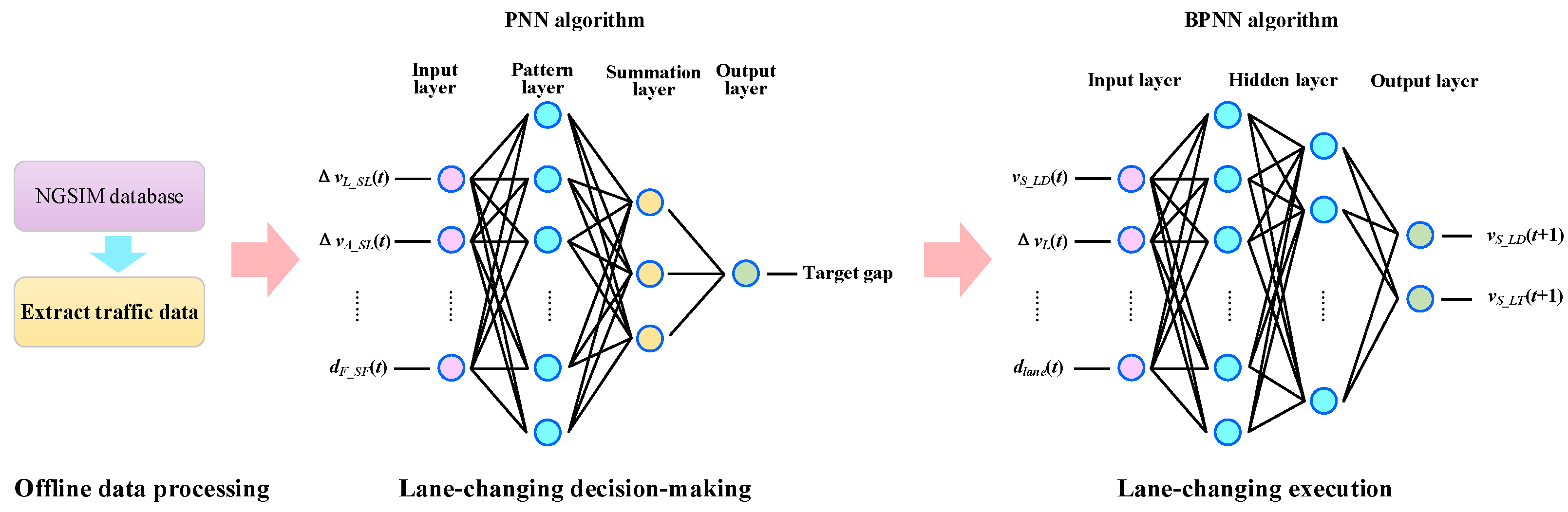
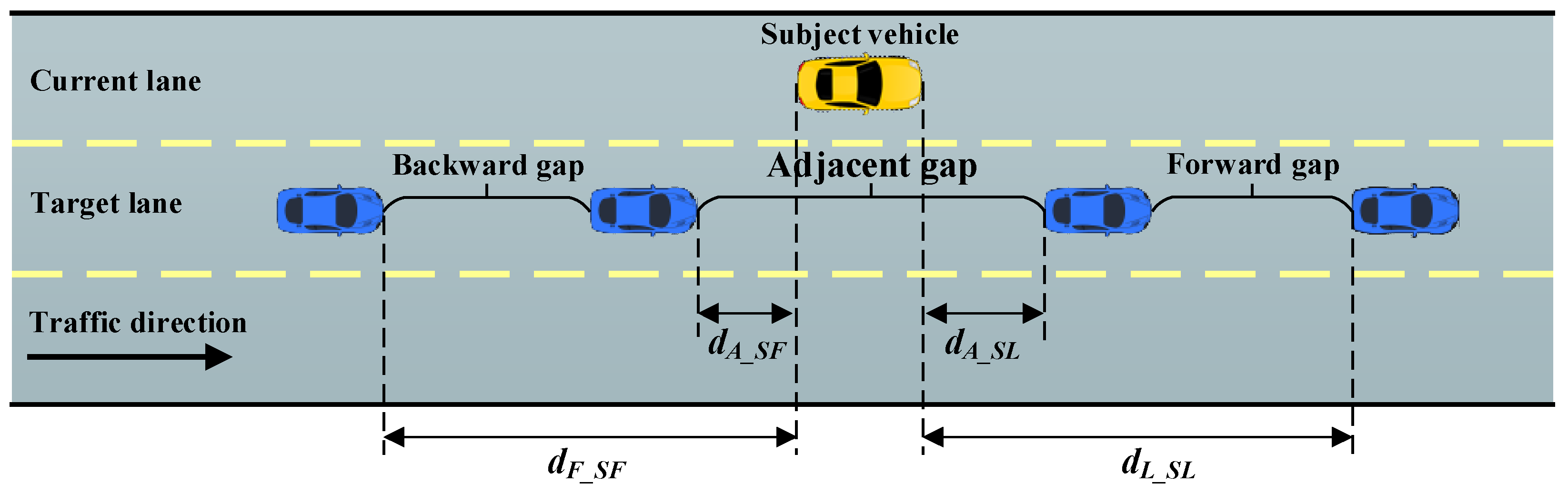
Lane-changing decision-making model: The PNN algorithm takes three kinds of gaps into consideration, including adjacent gap, backward gap, and forward gap in the target lane, as shown in Figure 3. Therefore, the problem is simplified to the “one out of three” choice of gaps for lane-changing. Specifically, the model is described as follows:

$$M_{{}_{out}}^{LCD}=F\left(M_{{}_{in}}^{LCD}\right)$$

(8)

$$M_{{}_{out}}^{LCD}\left(t\right)=\arg \underset{g}{\max }\left\{y_g\left(x\right)\right\}$$

(9)

$$M_{{}_{in}}^{LCD}\left(t\right)=\{\Delta v_{L\_SL},\Delta v_{A\_SL},\Delta v_{A\_SF},\Delta v_{F\_SF},d_{L\_SL},d_{A\_SL},d_{A\_SF},d_{F\_SF}\}$$

(10)

where $M_{{}_{in}}^{LCD}\left(t\right)$ is input and $M_{{}_{out}}^{LCD}\left(t\right)$ is the output of the algorithm at time t. Lane-changing decision-making process is denoted by F(·). The vector x represents all parameters for each lane change. The class g denotes the types of lane-changing gaps. G = {1, 2, 3}, which respectively represents forward gap, adjacent gap, and backward gap. Δv_{L_SL} is speed difference between the subject and leading vehicles in the forward gap. Δv_{A_SL} is speed difference between the subject and leading vehicles in the adjacent gap. Δv_{A_SF} is speed difference between the subject and following vehicles in the adjacent gap. Δv_{F_SF} is speed difference between the subject and following vehicles in the backward gap. Correspondingly, d_{L_SL}, d_{A_SL}, d_{A_SF}, and d_{F_SF} are distances between the subject vehicle and the four adjacent vehicles in the target lane.

The probability density function y_g(x) defines the concentration of the data of class g around the vector x, and it can be expressed as follows:

$$y_g\left(x\right)=\frac{1}{l_g{\left(2\pi \right)}^{n/2}{\displaystyle {\prod }_{j=1}^n{\delta }_j}}{\displaystyle \sum _{i=1}^{l_g}\exp \left(-{\displaystyle \sum _{j=1}^n\frac{{\left(x_{ij}^{\left(g\right)}-x_j\right)}^2}{2{\delta }_j^2}}\right)}$$

(11)

where σ_j is a smoothing parameter for the jth coordinate. l_g is the number of class examples. In the ith training vector, $x_{ij}^{\left(g\right)}$ denotes the jth element. i = 1, …, l_g. x_j is the jth coordinate of the vector x. Equation (11) aims to solve the “one out of three” problem.

(2)

Lane-changing execution model: When a vehicle starts to change to the target lane, it will interact with the leading and following vehicles in the target lane. Therefore, the parameters related to these vehicles have significant impact on lane-changing execution, such as speed difference and distance. General descriptions of the model are presented as follows:

$$M_{{}_{out}}^{LCE}=H\left(M_{{}_{in}}^{LCE}\right)$$

(12)

$$M_{{}_{out}}^{LCE}\left(t+1\right)=\{v_{S\_LD},v_{S\_LT}\}$$

(13)

$$M_{{}_{in}}^{LCE}\left(t\right)=\{v_{S\_LD},v_{S\_LT},\Delta v_L,\Delta v_F,d_L,d_F,d_{Lane}\}$$

(14)

where $M_{{}_{out}}^{LCE}\left(t+1\right)$ is the output at time t +1 and $M_{{}_{in}}^{LCE}\left(t\right)$ is the input at time t for the BPNN algorithm. H(·) denotes the function for lane-changing execution process. v_{S_LD} and v_{S_LT} represent respectively longitudinal and lateral speeds of the subject vehicle. Δv_L and Δv_F denote speed differences between the subject vehicle and the leader and follower vehicles in the target gap, respectively. d_L and d_F are distances between the subject vehicle and two adjacent vehicles in the target gap. d_Lane is the lateral distance to the target lane for the subject vehicle. Specifically, it denotes the minimum distance between the middle point of vehicle’s front bumper and the centerline of the target lane.

$$h_p^k=f\left(ne{t}_p^k\right)$$

(15)

$$ne{t}_p^k={\displaystyle \sum _{p=1}^{N_k}{W}_{pq}^k{h}_q^{k-1}+}{b}_p^k$$

(16)

$ne{t}_p^k$ and $h_p^k$ are the input and output of the pth neuron in the kth layer. f(·) denotes the activation function, and neurons of single hidden layer in this paper are activated with sigmoidal activation function. N_k is the number of neurons in the kth layer. $W_{pq}^k$ is the weight or strength of the connection between the pth and qth neurons. $b_p^k$ are the bias for the pth neuron in the kth layer. In this paper, the BPNN algorithm is designed with 3 hidden layers, and each hidden layer has 5 nodes.

2.3. Efficiency and Safety Evaluation Models

The road capacity is defined as the flow rate equivalent to the maximum 15-min moving average traffic count. To remove any random effects, each simulation is repeated by ten times, and the average value is treated as the final result.

$$C=q_{15\min }\times 4$$

(17)

where C represents the road capacity. q_15min denotes the maximum number of vehicles in a 15-min interval.

The index of time-to-collision (TTC) is one of most typical surrogate measures for traffic safety evaluation [27]. One TTC value can be calculated as follows:

$$TTC\left(i,t\right)=\frac{g\left(t\right)}{v\left(i,t\right)-v\left(i+1,t\right)}$$

(18)

where v(i, t) and v(i+1, t) are the speed of the subject and leading vehicles. According to the definition, a TTC value exists only when the subject vehicle is faster than the leader. Therefore, there is a constraint of v(i, t) > v(i+1, t).

The second index for safety evaluation is rear-end collision risk indexes (RCRI). It is based on an emergency condition, where a leading vehicle decelerates at the maximum deceleration rate. In this case, the subject vehicle has to brake to avoid a rear-end collision. The mathematical expression is as follows.

$$RCRI=\{\begin{array}{l}0, SS{D}_L>SS{D}_S\\ 1, SS{D}_L\le SS{D}_S\end{array}$$

(19)

$$M_{RCRI}=\frac{{\displaystyle \sum _{t=1}^T{\displaystyle \sum _{i=1}^{N}RCRI}}}{{\displaystyle \sum _{t=1}^T{\displaystyle \sum _{i=1}^{N}flag}}}$$

(20)

where SSD_L and SSD_S are safe stopping distance of the leading and subject vehicles, respectively. a_r is the deceleration and t_d is the delay before braking. T is the total time and N is the total number of vehicles. flag denotes the number of samples. M_RCRI is the average RCRI of all space-time points. According to a previous study [29], a_r = 3.4 m·s⁻² and t_d = 0.1 s.

Rear-end collision risk criteria for freeway safety can be stated in terms of the average RCRI as shown in

Table 1. Rear-end collision risk criteria.

Safety Level	MRCRI Range	Safety Level	MRCRI Range	Safety Level	MRCRI Range
A	[0, 0.251]	B	(0.251, 0.306]	C	(0.306, 0.355]
D	(0.355, 0.416]	E	(0.416, 0.510]	F	(0.510, 1]

[29].

3. Model Calibration and Testing

In this section, the proposed joint neural network model is calibrated and tested based on the NGSIM dataset. Specifically, 651 lane-changing samples are extracted. These selected lane-changing samples are randomly divided into two groups: 80% for training and 20% for testing. Moreover, two existing methods are used for comparison with our method. Bi et al. proposed a data-driven lane-changing model based on a randomized forest algorithm [30], while Sewall et al. used state-of-the-art agent-based models to simulate driver behaviors [31].

3.1. Test Results of Lane-Changing Decision-Making Model

As shown in

Table 2. Lane-changing decision-making result comparisons.

Groups	Backward Gap	Adjacent Gap	Forward Gap	Total
Ground truth traffic	30%	49%	21%	100%
Bi et al.’s method	17%	56%	27%	100%
Sewall et al.’s method	0%	100%	0%	100%
Our method	23%	51%	26%	100%

, 49% of vehicles prefer adjacent gap rather than the other two gaps in the real world. However, over 80% of vehicles choose adjacent and forward gaps for lane-changing in Bi et al.’s method. There are only 17% of vehicles choosing the backward gap, which reflects a clear difference in comparison with the ground truth traffic. In Sewall et al.’s method, all agent-based vehicles focus on the adjacent gap and completely ignore the other two gaps when there is lane-changing motivation. Obviously, these two methods have great disparity between them with the real world.

It is clear that results of our method are quite close to the ground truth traffic in terms of gap selection. About 26% of vehicles choose the forward gaps for changing their lanes and about half select the adjacent gaps. The remaining 23% of vehicles choose the backward ones. The largest difference occurs in the choice on backward gap, and the other two differences are lower than 6%. From this point of view, the proposed model is a suitable tool to simulate lane-changing decision-making behaviors.

3.2. Test Results of Lane-Changing Execution Model

In this part, Vehicle #2719 (V2719) and Vehicle #2823 (V2823) are chosen as examples. Figure 4 shows the speed comparisons in four scenarios, including the ground-truth from NGSIM dataset, Bi et al.’s method, Sewall et al.’s method, and our simulation results [30,31].

As shown in Figure 4a,d, the longitudinal speeds simulated by our method and Bi et al.’s method are significantly close to the ground truth traffic. However, Sewall et al.’s method cannot precisely capture lane-changing characteristics. Moreover, our method can produce more similar lane-changing trajectory patterns in terms of acceleration (V2719) or deceleration (V2832) processes. In Figure 4b,d, it is easier for all methods to extract the changes in lateral speed. For the lateral speed of V2719, Sewall et al.’s method seems to predict more accurately than Bi et al.’s. On the contrary, our method can reappear the changes of lateral speed during a lane change executed by the subject vehicle. Generally, our method shows the best performance in both longitudinal and lateral speeds.

Furthermore, Figure 5 shows the position comparison of three methods and the ground truth traffic. It consists of trajectory and gap. Each trajectory describes position changes in x- and y- axis directions, as shown in Figure 5a,c. Gap denotes the distance between the subject vehicle and the leader, as shown in Figure 5b,d. From the perspective of position, Figure 5 implies that the smallest difference can be observed between our method and the ground truth traffic. It is consistent with the findings in Figure 4.

Specifically, Figure 5a,c indicates that all three methods can track changes of direction, especially for V2719. Compared with Sewall et al.’s method, the other two methods show a shorter delay since the blue trajectory is above the others in each subfigure. The lines referred to Sewall et al.’s method present some fluctuations in Figure 5b,d. Contrarily, our method and Bi et al.’s method can provide a high-degree fitting in maintenance of the proper gap between the subject and leading vehicles. However, the former still has distinct advantages over the latter.

Generally, our method performs best in the test of lane-changing decision-making and execution models. Therefore, the calibration and test results demonstrate that the proposed joint neural network model is suitable for modeling traffic systems. In this paper, it also indirectly proves that the proposed model has the ability to simulate and predict the state of heterogeneous traffic.

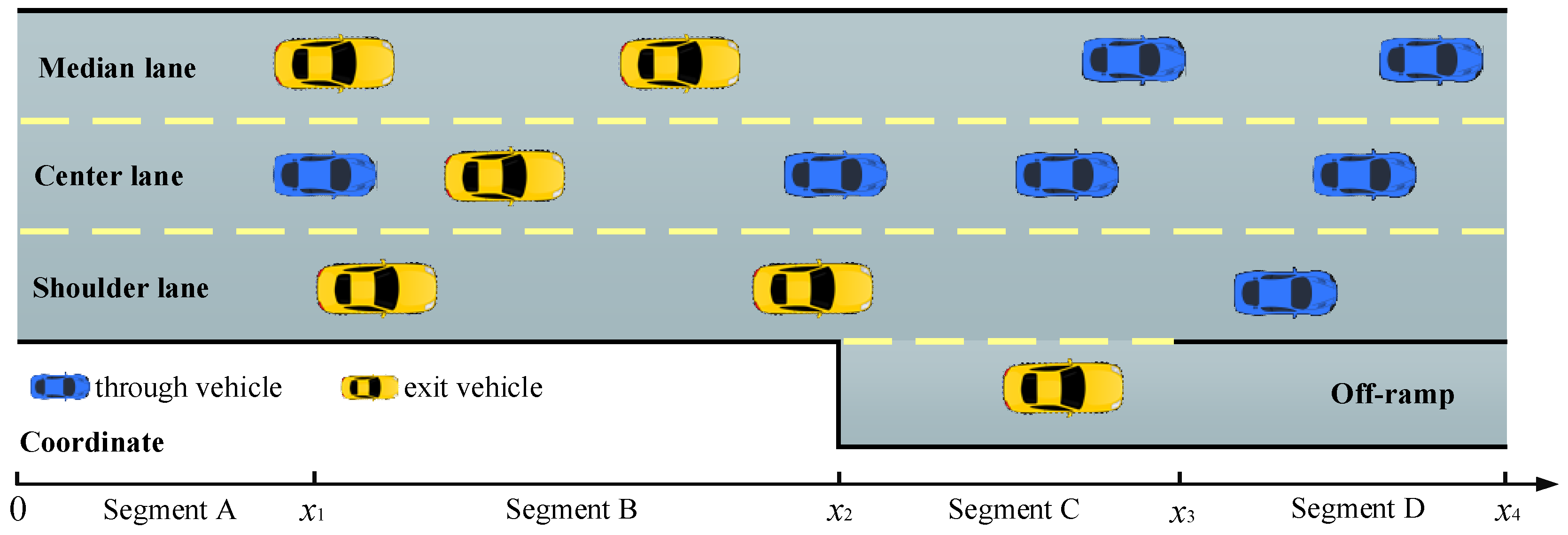
4. Simulation Preparations

Frequent lane-changing maneuvers at high traffic demand can be observed at an off-ramp bottleneck, especially at high traffic demand. As illustrated in Figure 6, the simulated scenario is a three-lane freeway, which has a one-lane off-ramp for exit vehicles.

The freeway contains four segments along the traffic direction. As shown in Figure 6, Segment A is the warm-up space for all vehicles. They can run at a desired and steady speed. In Segment B, exit vehicles intend to leave the mainline and change to the outer lanes, so there are frequent lane-changing movements in this segment. In this case, lane-changing models are used to control lateral trajectories. In order to avoid conflict with exit vehicles, through vehicles can only change to inner lanes both in Segment B and Segment C. Only through vehicles can be observed in Segment D, and thus only car-following models are applied in longitudinal control for MVs and IVs.

Simulation parameters are set as follows. The maximum speeds of mainline and ramps are 33 m/s and 22 m/s, respectively. (x₁, x₂, x₃, x₄) = (500, 1500, 1700, 2000) and the lane width is 3.6 m. Traffic demand is 1500 vehicles per hour per lane (vphpl). Additionally, the proportion of exit vehicles P_exit is 20% and they are evenly distributed in median, center and shoulder lanes.

5. Simulation Results and Discussion

After applying the proposed joint neural network model, we predict the state of future traffic flow and evaluate it from the aspects of speed, efficiency, and safety. The heterogeneous traffic flow consists of MVs and IVs. P_CACC denotes market penetration rate (MPR) of CACC vehicles. This section focuses on the impact of exit vehicles and CACC vehicles on evaluation indexes. In this case, P_CACC and P_exit are two key variables needed to be analyzed quantitatively at off-ramp bottlenecks.

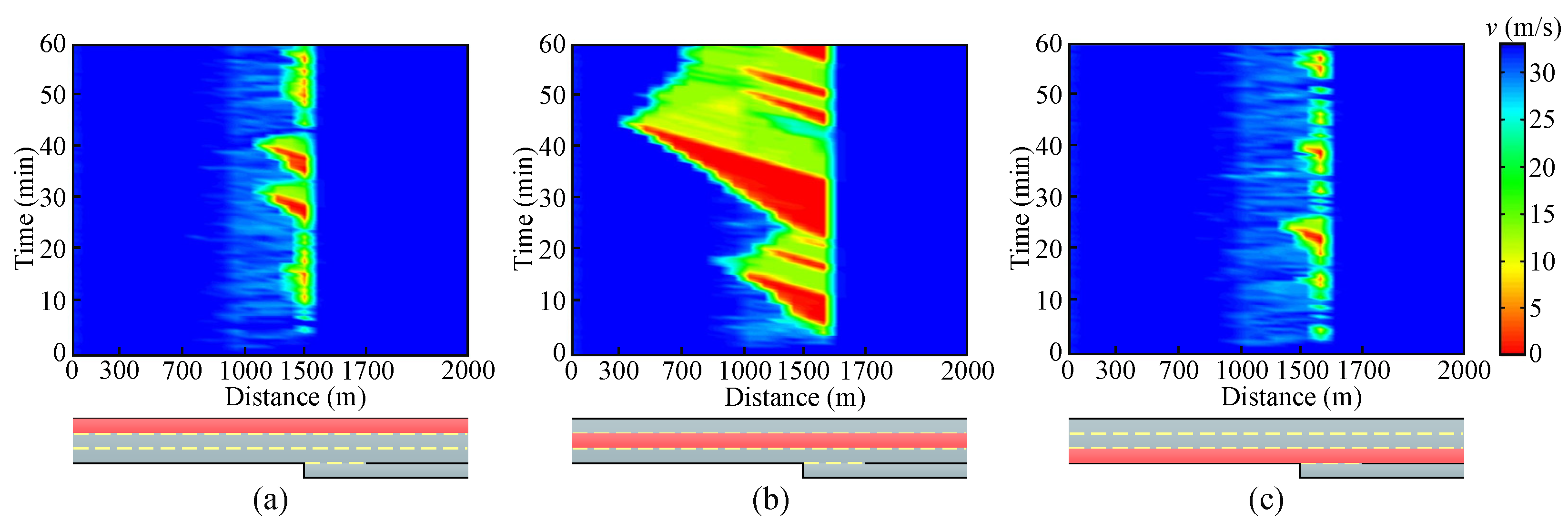
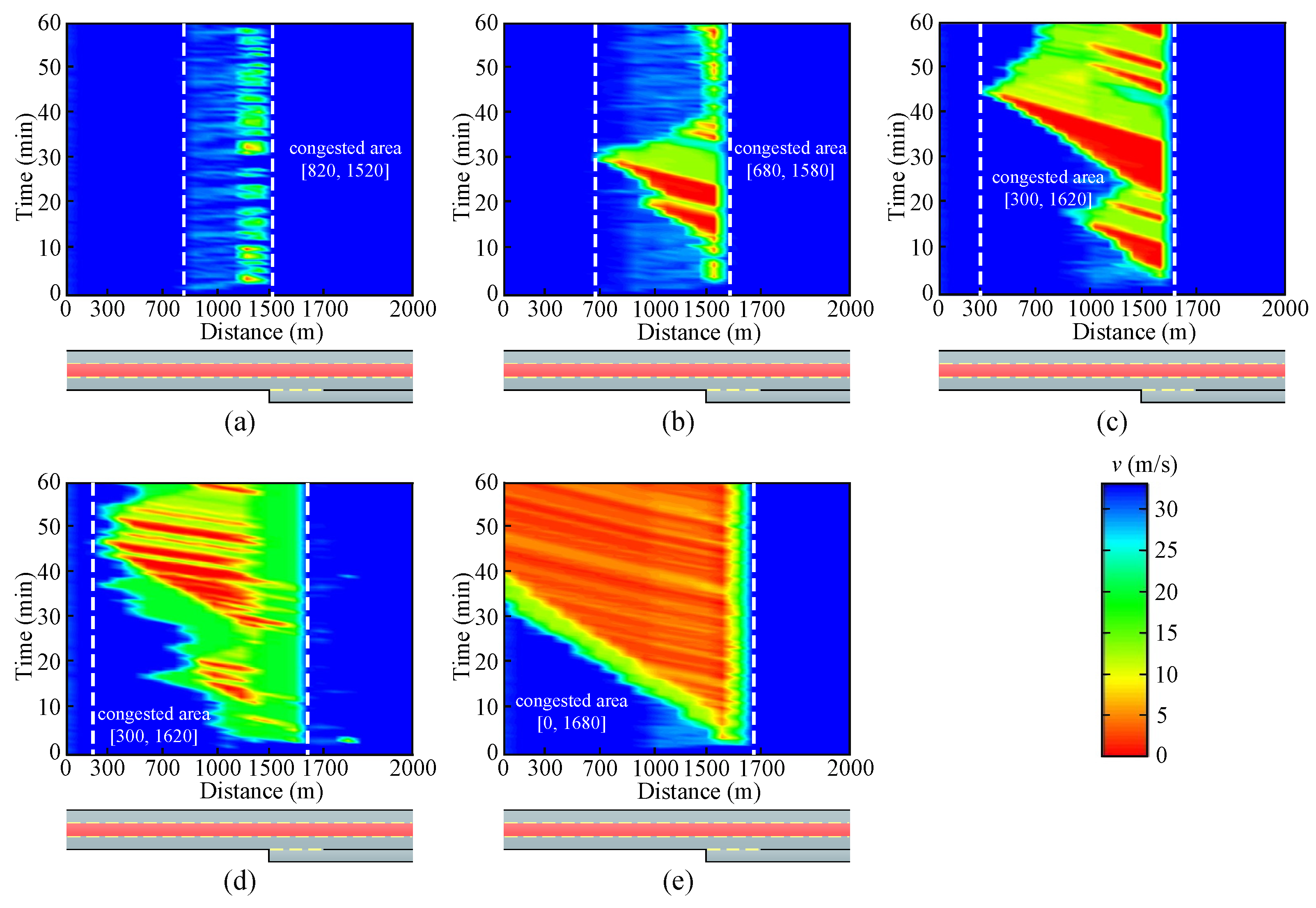
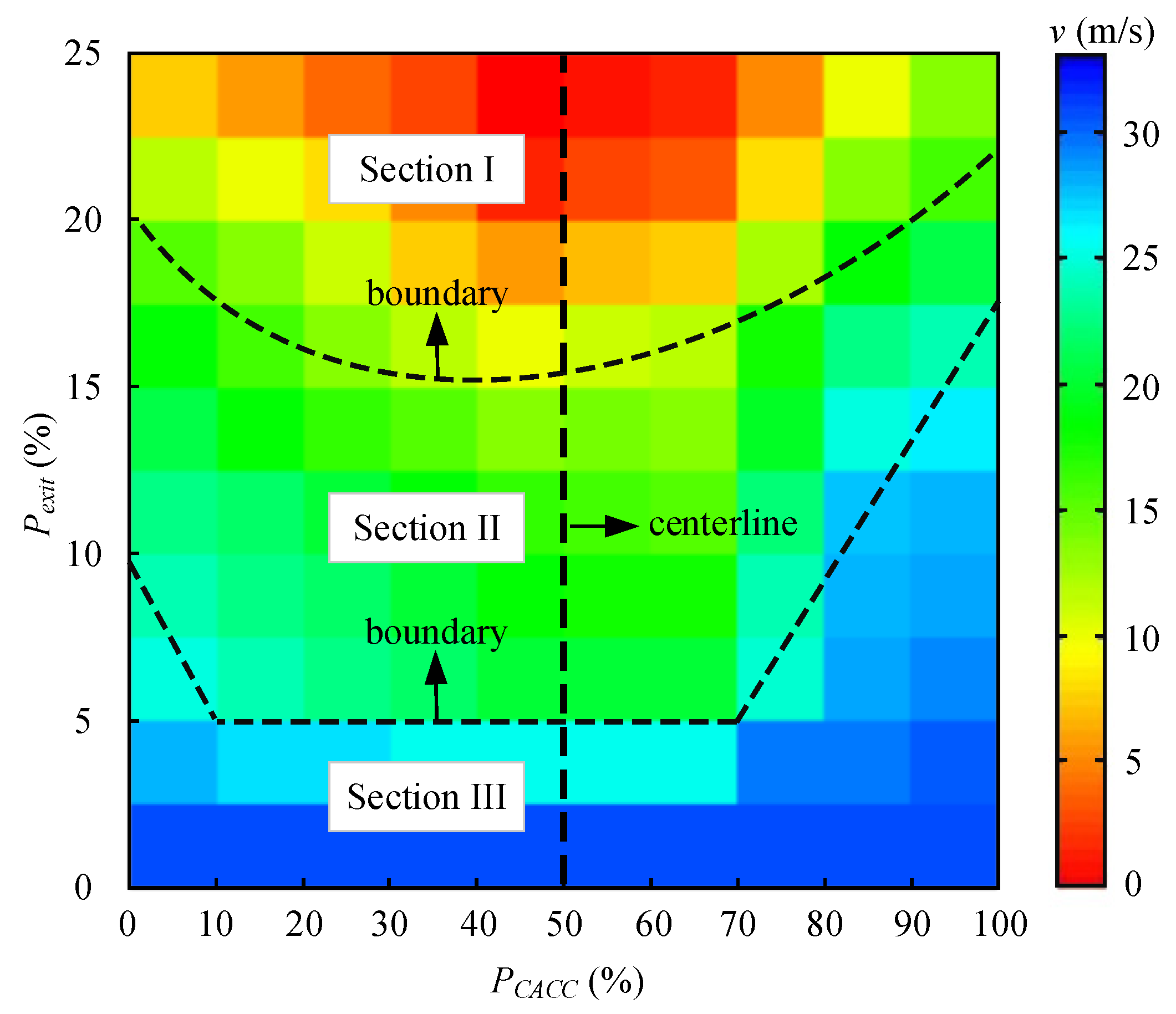
5.1. Impact on Average Speed

Figure 7 shows the spatiotemporal dynamics of average speed of three lanes in the mainline. In this group of experiments, P_CACC and P_exit are set to be 50% and 15%, respectively.

Obviously, lane-changing behaviors have negative impact on the traffic flow because they often produce some traffic interruptions and destroy the stability of the traffic flow. However, the impact varies in different lanes. For the median and shoulder lanes, the influencing areas begin at x = 1000 m and end at x = 1550 m. The congestion spontaneously dissipates quickly within the 550-m range. In the center lane, severe congestion tends to propagate upstream from x = 1600 m to even x = 300 m. From the perspective of propagation time, each shock wave lasts over 10 min in the center lane, while it decreases sharply to about one minute during congested periods in the other two lanes.

Moreover, average speeds of all lanes exceed 30 m/s in Segment A and Segment D, which means vehicles run at a desired speed. But in Segment B and Segment C, average speeds decrease remarkably because more and more exit vehicles change to target lanes. These vehicles may decelerate or even run at an extremely low speed until they find a proper gap. Taking the center lane as an example, the parts in red color indicate that average speeds are less than 10 m/s in congested areas. Although some jams occur within [1000 m, 1600 m] in the median and shoulder lanes, the traffic is still mildly congested. Generally, the traffic system is most vulnerable to the center lane in a congestion-prone condition.

Figure 8 shows the spatiotemporal patterns corresponding to the traffic breakdown and the transition from synchronized flow to jam. Vehicle trajectories in the center lane are displayed for 10 min within [500 m, 1000 m]. P_exit value maintains 15%. In contrast, P_CACC changes from 0 to 100% with a 20-percent interval. Clearly, the lane-changing influencing area gets bigger before P_CACC increases to 40%. One of the reasons for this congested phenomenon is that more and more ACC vehicles are degraded from CACC ones. Because of longer headway, ACC vehicles need more space in the target lane for lane changes. It is difficult to find a proper gap for lane-changing at the current speed, and thus deceleration potentially occurs during the lane-changing decision-making process. Meanwhile, congestions tend to propagate upstream, and the influencing area is approximately 200 m long, as shown in Figure 8c. Fortunately, such congestions can dissipate by themselves in near-term deployment scenarios where MPR of CACC vehicles is relatively low.

When P_CACC rises from 60% to 100%, the risk of congestion caused by forced lane changes gradually decreases. Specifically, the length of high-density area is limited to 200 m in Figure 8d, while congestion is suppressed around the position x = 1000 m. Additionally, typically short jams form in Figure 8e,f. Congestion hardly can be observed when P_CACC is more than 80%. Finally, traffic flow gradually becomes homogeneous when all vehicles are replaced by CACC vehicles.

Generally, lane-changing behaviors may induce severe congestions, especially when MPR of CACC vehicles ranges from 40% to 60%. Congestions resulting from forced lane-changing maneuvers propagate at upstream of the off-ramp bottleneck, and the length of influencing area is several hundred meters. The severity and propagation range are affected by at least two variables P_CACC and P_exit. However, congestions dissipate in the scenario with low P_CACC, where a transition from congested traffic to free flow can be observed clearly. Moreover, the traffic system with high P_CACC performs best since CACC vehicles help smooth the traffic flow by smaller headway and faster lane changes. This means that the negative impact of exit vehicles is compensated by the advantages of CACC vehicles to some extent.

Figure 9 shows the impact of P_exit on average speed in the center lane when the traffic demand is 1500 vphpl. P_exit increases from 5% to 25% with a 5-percentage interval. Obviously, exit vehicles have significant negative influence on the travel efficiency near the off-ramp. Increasing exit vehicles means more lane-changing requirements, which may cause deceleration. Because exit vehicles tend to slow down and look for a proper gap to change to the target lane, it easily results in severe upstream congestion of the off-ramp. In such heavy traffic, both lane-changing decision-making and execution processes are completed in low-speed state since localized jams cannot dissipate by themselves.

Specially, the congested area is within [820 m, 1520 m] and the average speed is over 15 m/s, when P_exit = 5%. The length of congested area respectively increases to 900 m and 1320 m, when P_exit rises to 10% and 15%. Red blocks in Figure 9c,d demonstrate that severe congestions occur in some areas, where average speeds are below 10 m/s. With the increase of P_exit value, more and more vehicles gather in the center lane. Moreover, lots of vehicles decelerate and queue at the off-ramp bottleneck. The jam waves propagate upstream and even affect the vehicle entrance at the starting point x = 0 m, as shown in Figure 9e.

Distribution of average speeds is summarized in Figure 10. Obviously, the smaller the P_exit value or the bigger the P_CACC value, the faster the average speed of all vehicles. Besides, Figure 10 is clearly divided into three sections: (1) average speeds in Section I are less than 10 m/s; (2) Section II denotes the average speeds ranged from 10 m/s to 25 m/s; and (3) the remaining are over 25 m/s in Section III. From a horizontal perspective, the boundary between Section I and Section II is approximately close to the horizontal line P_exit = 15%. Another boundary between Section II and Section III is the horizontal line P_exit = 5% when P_CACC is lower than 70%. Therefore, average speed is more sensitive to P_exit than P_CACC before CACC vehicles occupy a position of absolute predominance.

It is worth noting that the lowest speed always exists when P_CACC = 50%, as shown in the centerline of Figure 10. This means that MVs and IVs sharing the same MPR is the worst scenario. For the scenario with high MPR of CACC vehicles, the average speeds are even more than 25 m/s when P_exit ranges from 5% to 17.5%. In this case, these average speeds belong to Section II instead of Section III. Therefore, the distribution of these three sections is completely asymmetric. This finding indirectly demonstrates that CACC vehicles help to increase average speed and offset many negative effects of numerous lane change maneuvers at an upstream off-ramp.

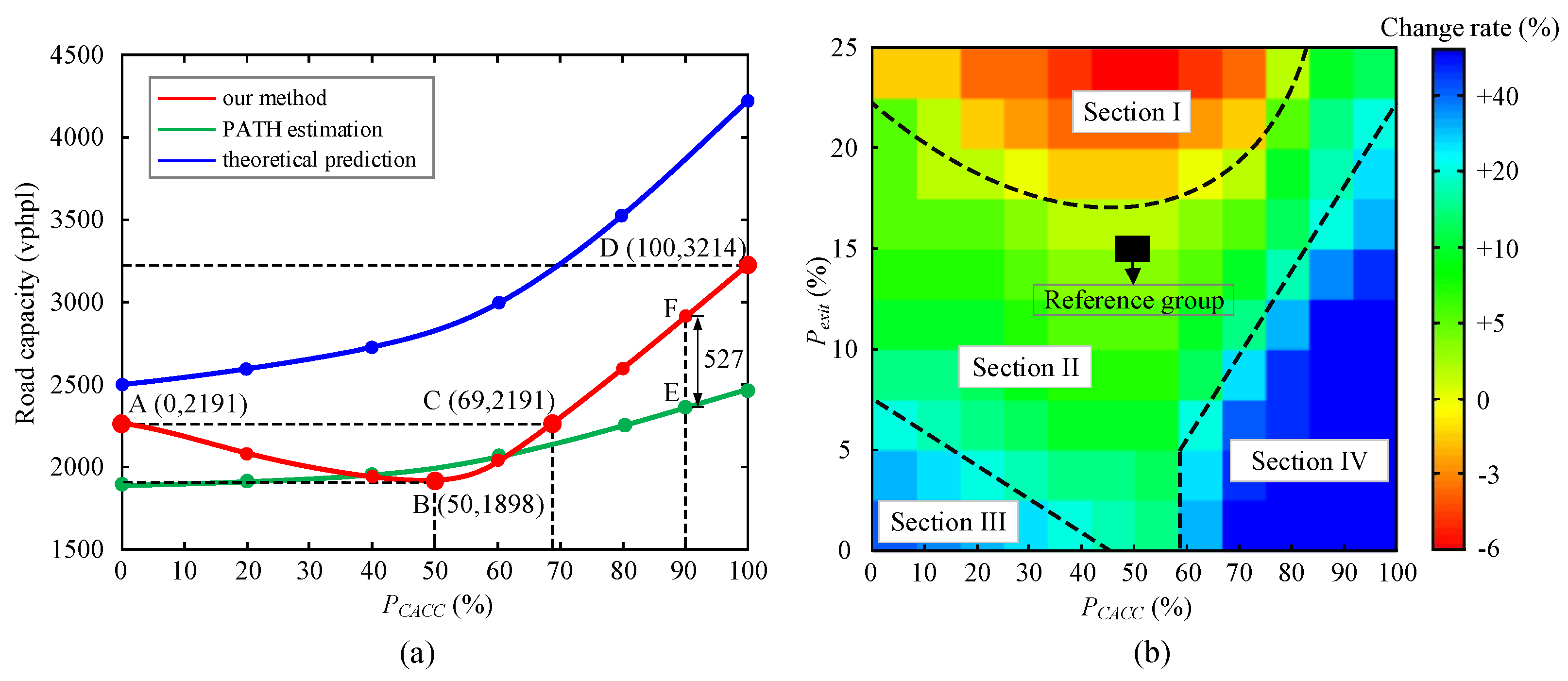
5.2. Impact on Road Capacity

Figure 11 presents the impact of MPR of CACC vehicles and proportion of exit vehicles on road capacity. The section chosen for capacity calculation is x = 2900 m in Figure 6. Simulation result of the proposed joint neural network is compared with that of PATH estimation and theoretical prediction [32], as shown in Figure 10. One can see that road capacity monotonically increases with the increase of P_CACC in the latter two methods, since CACC→ACC degradation is not taken into consideration. Results of theoretical prediction are remarkably higher than that of the other two methods. Moreover, the two lines denoting our method and PATH estimation are close to each other, and even partially intersecting.

Compared with theoretical prediction, the result of our method is much closer to that estimated by PATH, especially when P_CACC is within [0%, 70%]. Specifically, road capacity from PATH estimation is smaller than that from our method, but the gap between these two methods is narrowing before P_CACC increases to 40%. Conversely, the road capacity of our method is slightly lower than that of PATH estimation when P_CACC ranges from 40% to 60%. After that, road capacity increases rapidly to the maximum. Taking P_CACC = 90% as an example, the difference between our method and PATH estimation is 527 vphpl. Furthermore, the gap exceeds 700 vphpl when P_CACC = 100%. For theoretical prediction, road capacity increases from 2500 vphpl to over 4000 vphpl, since it neglects CACC→ACC degradation and strong negative disturbance of lane-changing maneuvers.

Particularly, the red line representing our method is divided into two parts. Road capacity decreases gradually from 2192 vphpl to 1898 vphpl before P_CACC rises to 50%. There is a 293-vphpl drop in amplitude, which is consistent with previous studies [15,23,33]. When P_CACC is increased from 50% to 100%, road capacity quickly reaches the peak of 3214 vphpl, which is improved by over 60% in comparison with the traffic scenario denoted by Point B in Figure 11a. It is worth noting that the two traffic scenarios share the same capacity in Point A and Point C, although the traffic flow components are quite different. It also proves indirectly that high-performance CACC vehicles help to overcome the drawbacks of CACC→ACC vehicles from an efficiency perspective.

Figure 11b presents the change rates of road capacity. The scenario of P_CACC = 50% and P_exit = 15% is treated as a reference group. Figure 11b is clearly divided into four sections. Section I denotes the worst scenarios compared with the reference group. These situations are associated with high proportion of exit vehicles, and moderate CACC MPR is also another important reason. The former refers to P_exit > 15% while the latter refers to P_CACC ∈ [0, 70%]. Likewise, the change rate ranges from 0% to 10% in Section II, and Section III represents the scenarios, where the change rate is within [10%, 30%]. Section II has the largest area. On the contrary, Section III includes the least cases and it is limited in a small triangle area, as shown in Figure 11b.

From the perspective of efficiency, the best section is Section IV, where the change rate of road capacity is over 30%. Obviously, it happens in the scenarios with low P_exit and high P_CACC. In this case, lane changes can hardly disrupt traffic flow and cause capacity reductions. If it happens in a short time, a large amount of vehicles of CACC vehicles ensure stability via smoothing the traffic flow. Therefore, it is necessary to take actions to increase MPR of CACC vehicles, such as vehicle technology innovation, media promotion, and financial subsidy on IVs.

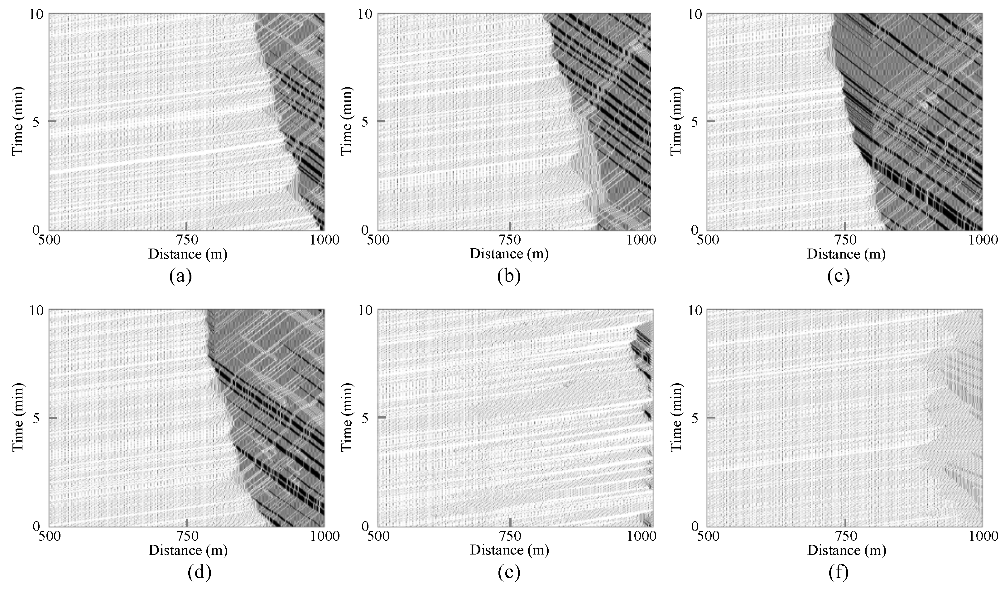
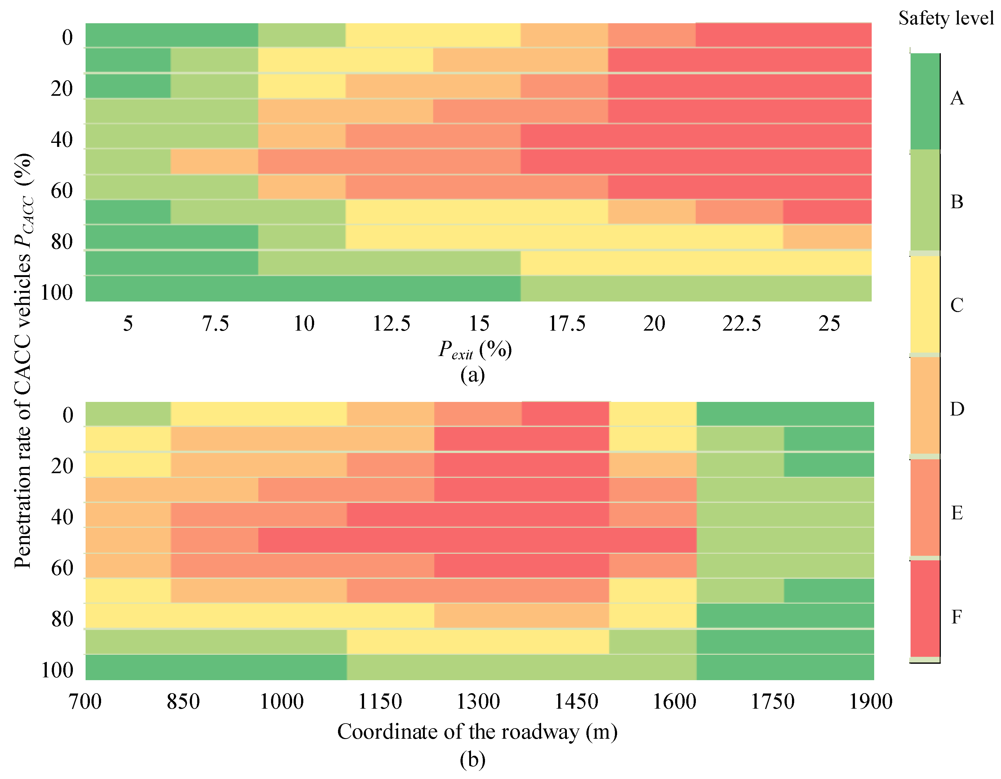
5.3. Impact on Safety

Furthermore, safety impact is evaluated using surrogate safety measures. TTC is one of the most typical parameters, and small TTC value means high collision risk. Figure 12 shows safety conditions in the four scenarios denoted by Points A, B, C, and D in Figure 10. TTC values are calculated for three lanes and mainline section.

Generally, travel safety condition in the center lane is apparently worse than that in the median and shoulder lanes, especially in Figure 12a,b. In contrast, safety performance in the shoulder lane is the best according to the severity and influencing area of low TTC value. For example, the red area in Figure 12(b3) is the shortest, which means vehicles run across this area at extremely high risk. For the other lanes, longer high-risk areas may bring about collision.

Specifically, the influencing area ranges from x = 800 m to x = 600 m, and the average TTC value is less than 1.5 s in the center lane. Besides, the range of high-risk area is [1300 m, 1600 m], and TTC value is even less than 0.5 s. But for the other lanes, the influencing area is smaller and starts from 1150 m. Moreover, average TTC values in the median and shoulder lanes are about 1.5 s. The extremely high-risk conditions only exist within two hundred meters or less at spatial scale.

Similarly, each lane shares the same trend in the change of TTC values. One can see that TTC values get smaller when vehicles are close to the off-ramp. This is due to narrower gaps for lane-changing before the off-ramp bottleneck, which is also one of the reasons for rear-end collision. As shown in Figure 12a,c, the two scenarios differ from each other in terms of safety, although they obtain the same road capacity at Point A and Point C. Taking the center lane as an example, the TTC value is significantly higher than 0.5 s in the range of [1300 m, 1600 m], as shown in Figure 12(c2). In contrast, the safety condition in Point A is worse than that in Point C.

For the mainline section, the change trend is consistent with that of the center lane. The influencing area ranges from x = 1000 m to x = 1600 m, and the high-risk area is within [1300 m, 1600 m]. For the starting point of influencing area, it only covers about 100 m in Point B. Compared with Point B, Point D with more CACC vehicles shows the minimum risk. However, when P_CACC rises from 0 in Point A to 50% in Point B, safety performance of the traffic system decreases. During this process, more ACC vehicles exist and they have higher requirements on gaps for lane-changing. It may result in high deceleration rates, and even queuing in the current lane. Finally, exit vehicles spend more time changing to the target lane at low speed in a congested scenario. Generally, the longer duration time and smaller gaps of lane-changing maneuvers imply higher risk. It can easily lead to a decrease in TTC value, and even collisions in a high-density traffic flow, especially at upstream of the off-ramp.

Figure 13 shows the distribution of safety levels from two aspects. In Figure 13a, safety levels vary with the two key variables, P_exit and P_CACC. The distribution of Level E and Level F shows a pyramid-shaped structure with the increase of P_exit. However, the center of the bottom is chosen to the scenarios with low MPR of CACC vehicles. When P_CACC is within [30%, 60%], the safety level is mainly B in the scenarios of P_exit < 10%. It is downgraded to Level D and Level E when P_exit rises to 10%–15%. Eventually, the highest-risk level F accounts for the majority of all safety levels when P_exit is over 17.5%. Therefore, with increase of exit vehicles, more and more lane-changing maneuvers cause frequent variation of gaps and speeds, resulting in higher driving risk. However, when P_exit reaches 25%, safety level is upgraded from F to D by increasing P_CACC to more than 80%.

Taking P_exit = 15% as an example, Figure 13b presents the distribution of safety levels along the roadway. Obviously, the safety level distribution is asymmetric, and safety levels in the lower half of the distribution are remarkably better than those in the upper half. In detail, high-risk areas are concentrated in [1000 m, 1600 m], while Level F ranges from 1300 m to 1600 m, which is consistent with the findings in Figure 11. With the increase of P_CACC, the safety level is gradually upgraded from F to B within [1000 m, 1600 m]. When vehicles run downstream the off-ramp, the traffic flow becomes free flow after x = 1700 m. In this area, lane-changing maneuvers decrease significantly and safety is also improved to Level A/B.

6. Conclusions

The goal of this paper is to use neural network algorithms to imitate lane-changing behaviors. PNN and BPNN are respectively chosen to learn lane-changing decision-making and execution processes. The validation of the proposed method is demonstrated in comparison with the truth traffic and two selected methods. A freeway with three main-line lanes and a one-lane off-ramp is designed as the simulation site. Numerical simulation experiments are conducted to evaluate the traffic system in terms of efficiency and safety. The major results are concluded as follows:

(1)

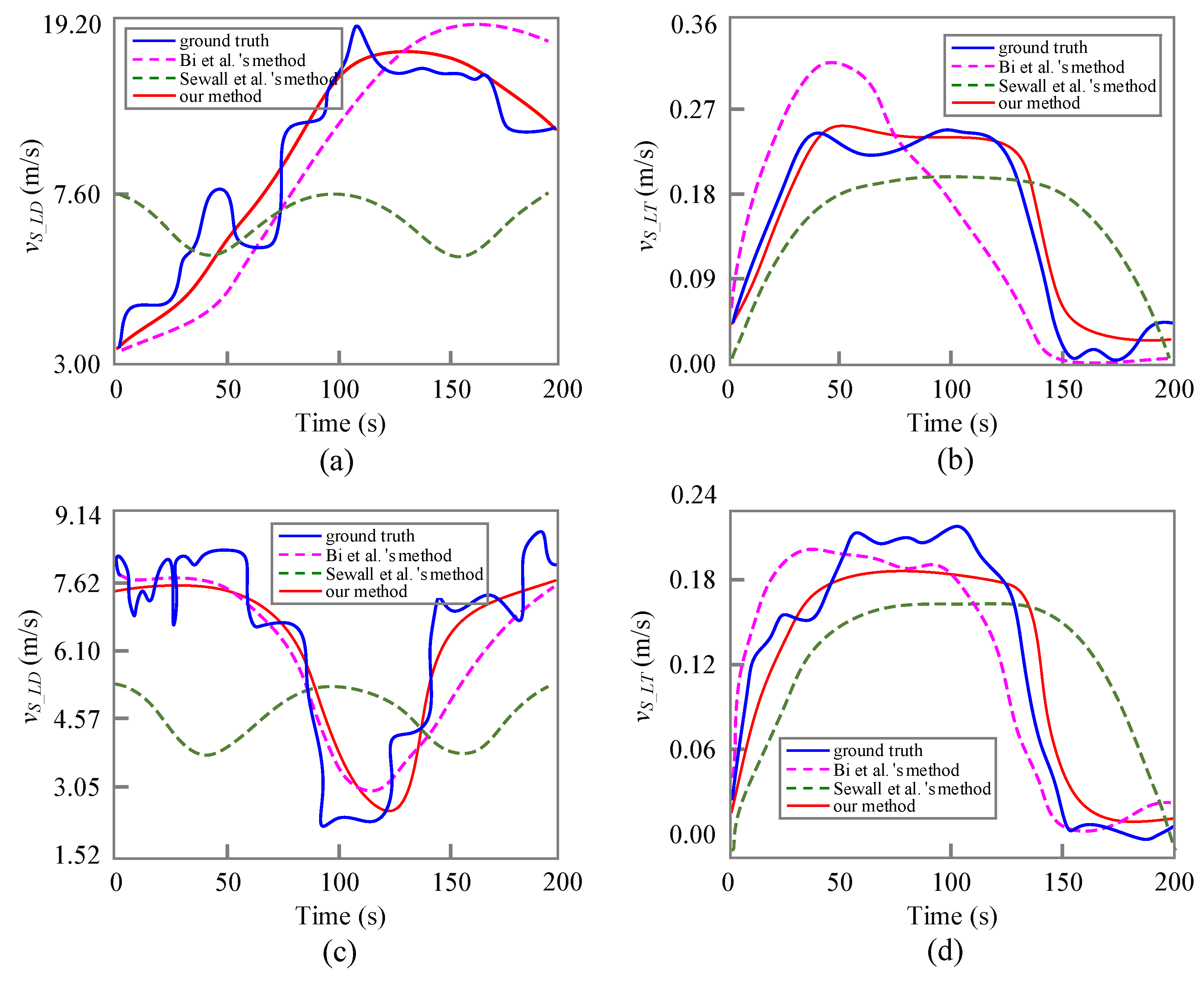
The proposed hybrid neural network has distinct advantages over the two existing methods. Compared with the ground truth traffic, our method can accurately predict required gap for a lane change. Moreover, trajectories controlled by our method are evidently closer to the ones extracted from NGSIM dataset during lane-changing execution.

(2)

Based on car-following and lane-changing models, a simulation platform is established to investigate various traffic scenarios. The results indicate that the center lane is the most delicate lane near an off-ramp bottleneck. Frequent lane-changing maneuvers have the most negative impact on the center lane in terms of congestion severity. When P_CACC is 50%, average speed in the center lane is dropped to 10 m/s with the increase of P_exit value. Moreover, severe congestions even cannot dissipate spontaneously at upstream of the off-ramp. In this case, decreasing P_exit or increasing P_CACC is an efficient solution for traffic congestion reduction. The former can be realized by route guidance in a traffic network, while the latter makes full use of smaller headway and faster reaction of CACC vehicles.

(3)

The results of evaluation performance on road capacity and travel safety are quite sensitive to the values of P_CACC and P_exit. When P_CACC = 100%, road capacity reaches the peak 3214 vphpl, while the minimum is less than 1900 vphpl with 50% of CACC vehicles in the traffic system. For safety evaluation, when vehicles run within 600 m at upstream of the off-ramp, drivers and passengers are at the greatest risk of collision involvement. However, when P_CACC is greater than 80% or P_exit is lower than 15%, the safety level is significantly improved from Level E to Level B.

(4)

Degradation of CACC performance is considered in this paper. So, the number of ACC vehicles reaches the maximum value when IVs and MVs account for half of the motor vehicle market. Furthermore, ACC vehicles require the longest headway in comparison with CACC vehicles and MVs. During a lane-changing process, ACC vehicles need the biggest headway gap between its leading vehicle and following one in the target lane. Therefore, CACC→ACC degradation can result in worse performance on efficiency and safety. Besides increasing more CACC vehicles, communication facilities equipped in more MVs also contribute to a better traffic system.

In our future work, the following aspects need more attention: (1) This paper only focuses on the comparison of lane-changing trajectories between different methods, and hence, the performance of traffic system controlled by different methods should be studied and analyzed in future research. (2) Besides travel efficiency and safety, fuel consumption and vehicular emissions at the freeway bottleneck should be also further evaluated. (3) The practicability of the proposed models should be verified in other environments, such as two-lane freeway, on-ramp bottlenecks and emergency scenarios.

References

1. Shladover, S.E. Connected and automated vehicle systems: Introduction and overview. J. Transp. Syst. 2018, 22, 190–200. [Google Scholar] [CrossRef]
2. Wang, Z.; Shi, X.; Li, X. Review of Lane-Changing Maneuvers of Connected and Automated Vehicles: Models, Algorithms and Traffic Impact Analyses. J. Indian Inst. Sci. 2019, 99, 589–599. [Google Scholar] [CrossRef]
3. Shi, Y.; Yuan, Z.; Yu, H.; Guo, Y.; Qi, Y. A Graph-Based Optimal On-Ramp Merging of Connected Vehicles on the Highway. Machines 2021, 9, 290. [Google Scholar] [CrossRef]
4. Ji, A.; Levinson, D. A review of game theory models of lane changing. Transp. A Transp. Sci. 2020, 16, 1628–1647. [Google Scholar] [CrossRef]
5. Kesting, A.; Treiber, M.; Helbing, D. Enhanced intelligent driver model to access the impact of driving strategies on traffic capacity. Philos. Trans. R. Soc. London. Ser. A Math. Phys. Eng. Sci. 2010, 368, 4585–4605. [Google Scholar] [CrossRef] [PubMed] [Green Version]
6. Bai, Y.; Zhang, Y.; Li, X.; Hu, J. Cooperative weaving for connected and automated vehicles to reduce traffic oscillation. Transp. A Transp. Sci. 2019, 1–19. [Google Scholar] [CrossRef]
7. Ma, J.; Che, X.; Li, Y.; Lai, E.M.-K. Traffic Scenarios for Automated Vehicle Testing: A Review of Description Languages and Systems. Machines 2021, 9, 342. [Google Scholar] [CrossRef]
8. Shladover, S.E.; Su, D.; Lu, X.-Y. Impacts of Cooperative Adaptive Cruise Control on Freeway Traffic Flow. Transp. Res. Rec. J. Transp. Res. Board 2012, 2324, 63–70. [Google Scholar] [CrossRef] [Green Version]
9. Milanés, V.; Shladover, S.E. Modeling cooperative and autonomous adaptive cruise control dynamic responses using experimental data. Transp. Res. Part C Emerg. Technol. 2014, 48, 285–300. [Google Scholar] [CrossRef] [Green Version]
10. Bouadi, M.; Jia, B.; Jiang, R.; Li, X.; Gao, Z. Optimizing sensitivity parameters of automated driving vehicles in an open heterogeneous traffic flow system. Transp. A Transp. Sci. 2021, 1–45. [Google Scholar] [CrossRef]
11. Ye, L.; Yamamoto, T. Impact of dedicated lanes for connected and autonomous vehicle on traffic flow throughput. Phys. A Stat. Mech. Its Appl. 2018, 512, 588–597. [Google Scholar] [CrossRef]
12. Ye, L.; Yamamoto, T. Modeling connected and autonomous vehicles in heterogeneous traffic flow. Phys. A Stat. Mech. Its Appl. 2018, 490, 269–277. [Google Scholar] [CrossRef]
13. Arvin, R.; Khattak, A.J.; Kamrani, M.; Rio-Torres, J. Safety evaluation of connected and automated vehicles in mixed traffic with conventional vehicles at intersections. J. Intell. Transp. Syst. 2021, 25, 170–187. [Google Scholar] [CrossRef]
14. Wang, H.; Qin, Y.; Wang, W.; Chen, J. Stability of CACC-manual heterogeneous vehicular flow with partial CACC performance degrading. Transp. B Transp. Dyn. 2019, 7, 788–813. [Google Scholar] [CrossRef]
15. Mahdinia, I.; Arvin, R.; Khattak, A.J.; Ghiasi, A. Safety, Energy, and Emissions Impacts of Adaptive Cruise Control and Cooperative Adaptive Cruise Control. Transp. Res. Rec. J. Transp. Res. Board 2020, 2674, 253–267. [Google Scholar] [CrossRef]
16. Gipps, P. A model for the structure of lane-changing decisions. Transp. Res. Part B Methodol. 1986, 20, 403–414. [Google Scholar] [CrossRef]
17. Dong, C.; Wang, H.; Li, Y.; Wang, W.; Zhang, Z. Route Control Strategies for Autonomous Vehicles Exiting to Off-Ramps. IEEE Trans. Intell. Transp. Syst. 2020, 21, 3104–3116. [Google Scholar] [CrossRef]
18. Kesting, A.; Treiber, M.; Helbing, D. General Lane-Changing Model MOBIL for Car-Following Models. Transp. Res. Rec. J. Transp. Res. Board 2007, 1999, 86–94. [Google Scholar] [CrossRef] [Green Version]
19. Toledo, T.; Choudhury, C.F.; Ben-Akiva, M.E. Lane-changing model with explicit target lane choice. Transp. Res. Rec. 2005, 1934, 157–165. [Google Scholar] [CrossRef]
20. Shamir, T. How Should an Autonomous Vehicle Overtake a Slower Moving Vehicle: Design and Analysis of an Optimal Trajectory. IEEE Trans. Autom. Control 2004, 49, 607–610. [Google Scholar] [CrossRef]
21. Yang, D.; Zheng, S.; Wen, C.; Jin, P.J.; Ran, B. A dynamic lane-changing trajectory planning model for automated vehicles. Transp. Res. Part C Emerg. Technol. 2018, 95, 228–247. [Google Scholar] [CrossRef]
22. Dong, C.; Wang, H.; Li, Y.; Shi, X.; Ni, D.; Wang, W. Application of machine learning algorithms in lane-changing model for intelligent vehicles exiting to off-ramp. Transp. A Transp. Sci. 2021, 17, 124–150. [Google Scholar] [CrossRef]
23. Mahajan, V.; Katrakazas, C.; Antoniou, C. Prediction of Lane-Changing Maneuvers with Automatic Labeling and Deep Learning. Transp. Res. Rec. J. Transp. Res. Board 2020, 2674, 336–347. [Google Scholar] [CrossRef]
24. Das, A.; Khan, N.; Ahmed, M.M. Detecting lane change maneuvers using SHRP2 naturalistic driving data: A comparative study machine learning techniques. Accid. Anal. Prev. 2020, 142, 105578. [Google Scholar] [CrossRef]
25. Xie, D.-F.; Fang, Z.-Z.; Jia, B.; He, Z. A data-driven lane-changing model based on deep learning. Transp. Res. Part C Emerg. Technol. 2019, 106, 41–60. [Google Scholar] [CrossRef]
26. Minderhoud, M.M.; Bovy, P.H. Extended time-to-collision measures for road traffic safety assessment. Accid. Anal. Prev. 2001, 33, 89–97. [Google Scholar] [CrossRef]
27. Li, Y.; Tu, Y.; Fan, Q.; Dong, C.; Wang, W. Influence of cyber-attacks on longitudinal safety of connected and automated vehicles. Accid. Anal. Prev. 2018, 121, 148–156. [Google Scholar] [CrossRef]
28. NGSIM—Next Generation SIMulation. 2013. Available online: https://ops.fhwa.dot.gov/trafficanalysistools/ngsim.htm (accessed on 15 July 2013).
29. Oh, C.; Park, S.; Ritchie, S. A method for identifying rear-end collision risks using inductive loop detectors. Accid. Anal. Prev. 2006, 38, 295–301. [Google Scholar] [CrossRef]
30. Bi, H.; Mao, T.; Wang, Z.; Deng, Z. A data-driven model for lane-changing in traffic simulation. Symp. Comput. Animat. 2016, 149–158. [Google Scholar]
31. Sewall, J.; Berg, J.V.D.; Lin, M.C.; Manocha, D. Virtualized Traffic: Reconstructing Traffic Flows from Discrete Spatiotemporal Data. IEEE Trans. Vis. Comput. Graph. 2010, 17, 26–37. [Google Scholar] [CrossRef] [Green Version]
32. Liu, H.; Kan, X.D.; Shladover, S.E.; Lu, X.-Y.; Ferlis, R.E. Modeling impacts of Cooperative Adaptive Cruise Control on mixed traffic flow in multi-lane freeway facilities. Transp. Res. Part C Emerg. Technol. 2018, 95, 261–279. [Google Scholar] [CrossRef]
33. Ioannou, P.; Stefanovic, M. Evaluation of ACC Vehicles in Mixed Traffic: Lane Change Effects and Sensitivity Analysis. IEEE Trans. Intell. Transp. Syst. 2005, 6, 79–89. [Google Scholar] [CrossRef] [Green Version]
Figure 1. Freeway sites where NGSIM vehicle trajectory data are obtained.
Machines 10 00109 g001
Figure 2. Pipeline illustration of a joint neural network model.
Machines 10 00109 g002
Figure 3. Schematic illustration of the lane-changing model.
Machines 10 00109 g003
Figure 4. Speed comparison of different methods. (a,b) respectively denote the longitudinal and lateral speeds of V2719. (c,d) respectively denote the longitudinal and lateral speeds of V2823.
Machines 10 00109 g004
Figure 5. Position comparison of different methods. (a,c) respectively denote trajectories of V2719 and V2823. (b,d) respectively denote the gaps to the leader for V2719 and V2823.
Machines 10 00109 g005
Figure 6. Coordinate system and frame of simulation freeway with an off-ramp.
Machines 10 00109 g006
Figure 7. Characteristics of average speed in different lanes. Characteristics of average speed in different lanes. (ac) respectively the median, center and shoulder lanes.
Machines 10 00109 g007
Figure 8. Temporal-spatial pattern of vehicle trajectories. (a) PCACC=0, (b) PCACC=20%, (c) PCACC=40%, (d) PCACC=60%, (e) PCACC=80%, and (f) PCACC=100%.
Machines 10 00109 g008
Figure 9. Spatiotemporal dynamics of average speed in the center lane. (a) Pexit = 5%,(b) Pexit = 10%, (c) Pexit = 15%, (d) Pexit = 20%, and (e) Pexit = 25%.
Machines 10 00109 g009
Figure 10. Summary of average speed in different traffic scenarios.
Machines 10 00109 g010
Figure 11. Road capacities in different traffic scenarios. (a) denotes capacity changes over PCACC, and (b) denotes capacity change rates over PCACC and Pexit.
Machines 10 00109 g011
Figure 12. Average TTC values in different lanes. (a1)–(d1) denote median lane, (a2)–(d2) denote center lane, (a3)–(d3) denote shoulder lane and (a4)–(d4) denote mainline section.
Machines 10 00109 g012
Figure 13. Distribution of safety levels. (a) denotes the distribution of safety levels over PCACC and Pexit, and (b) denotes the distribution of safety levels along the roadway.
Machines 10 00109 g013