


Research on a Visual Servoing Control Method Based on Perspective Transformation under Spatial Constraint


Abstract
1. Introduction
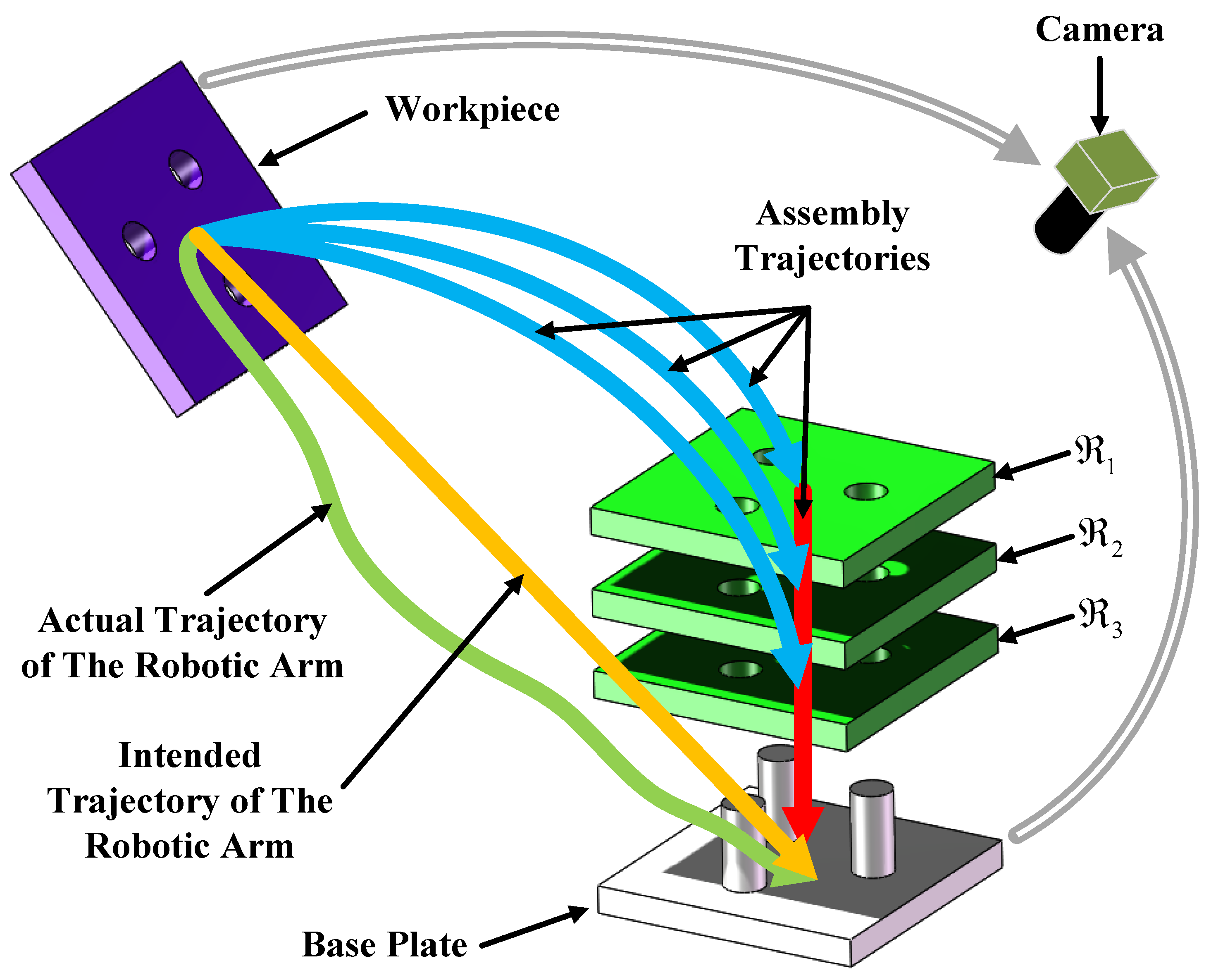
2. Problem Statements
3. Visual Servoing Control Method Based on Perspective Transformation
3.1. Methodology
- (1)
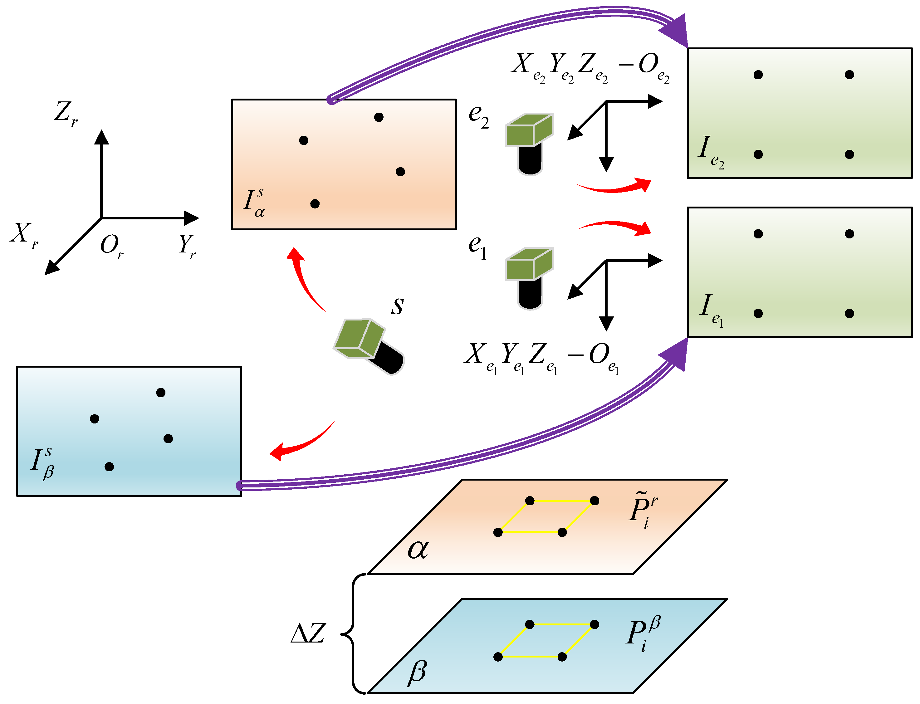
- A virtual image plane is generated, and then two homography matrixes and are established.
- (2)
- Assuming that and are the projections of spatial points and , respectively, in an image. Then, using matrix to map into the virtual image plane , a new feature is created. In the same way, mapping into the virtual image plane with yields a new feature . When , we believe that deviates from exclusively in the direction of the Z-axis. If represents a set of feature points on the workpiece and represents the corresponding feature points on the base plate, when equals , the workpiece has already arrived at the assembly node.
- (3)
- Assuming that the workpiece is located on the end-effector of a robotic arm. After that, the attitude of the end-effector is extracted, and the robotic arm is driven along a linear trajectory under the attitude, thereby docking the workpiece with the base plate.
3.2. Feasibility Analysis
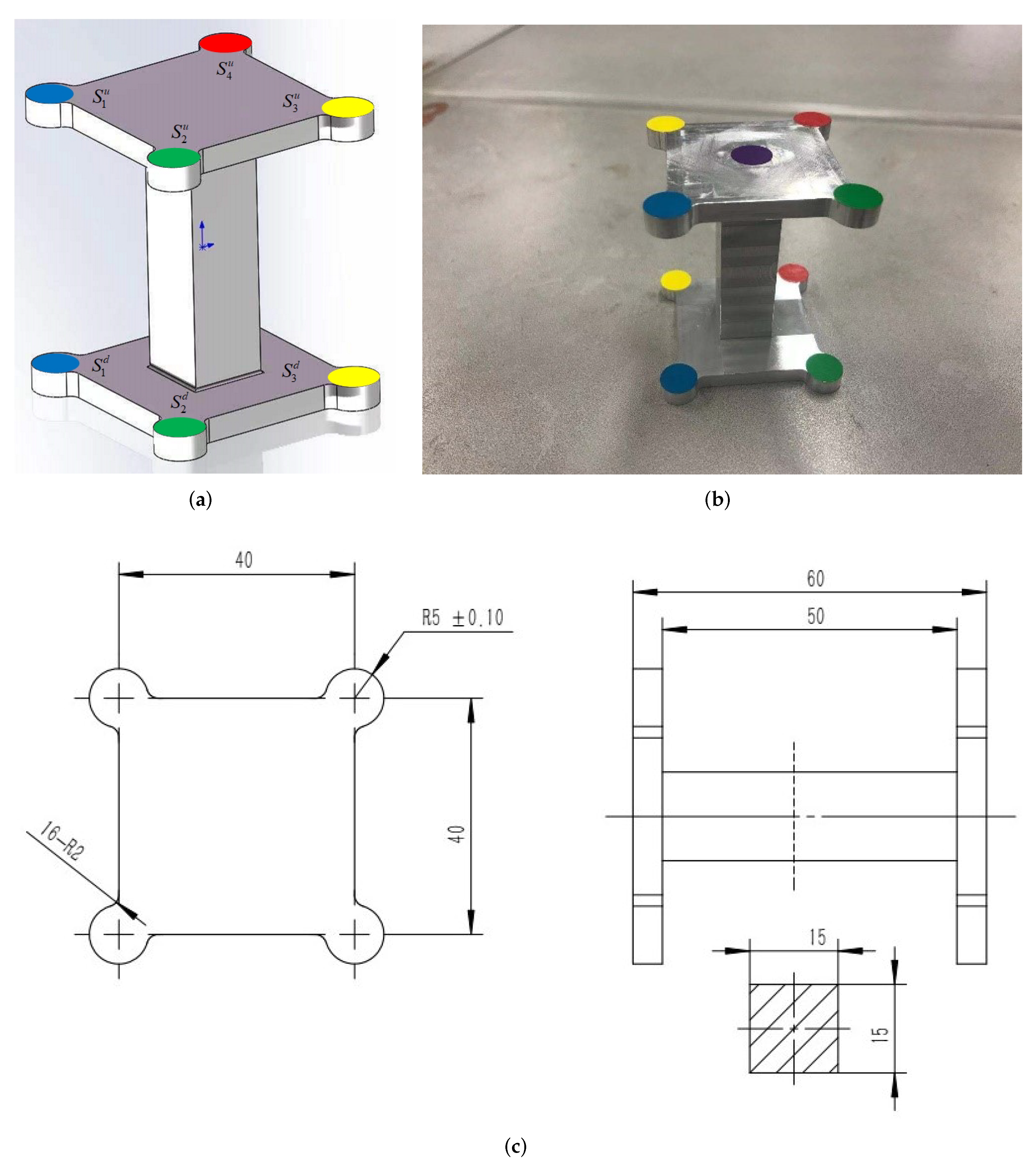
3.3. Calculation of the Transformation Matrix
- (1)
- Creating a square with a side length of d and retrieving all of its corners points , where represents the four upper corner points, and represents the four lower corner points. The corresponding image points and can be extracted using the image processing approaches.
- (2)
- A virtual image plane is created, and four image points forming a square are selected.
- (3)
- The transformational matrix and can be obtained by substituting , and DLT method, respectively.
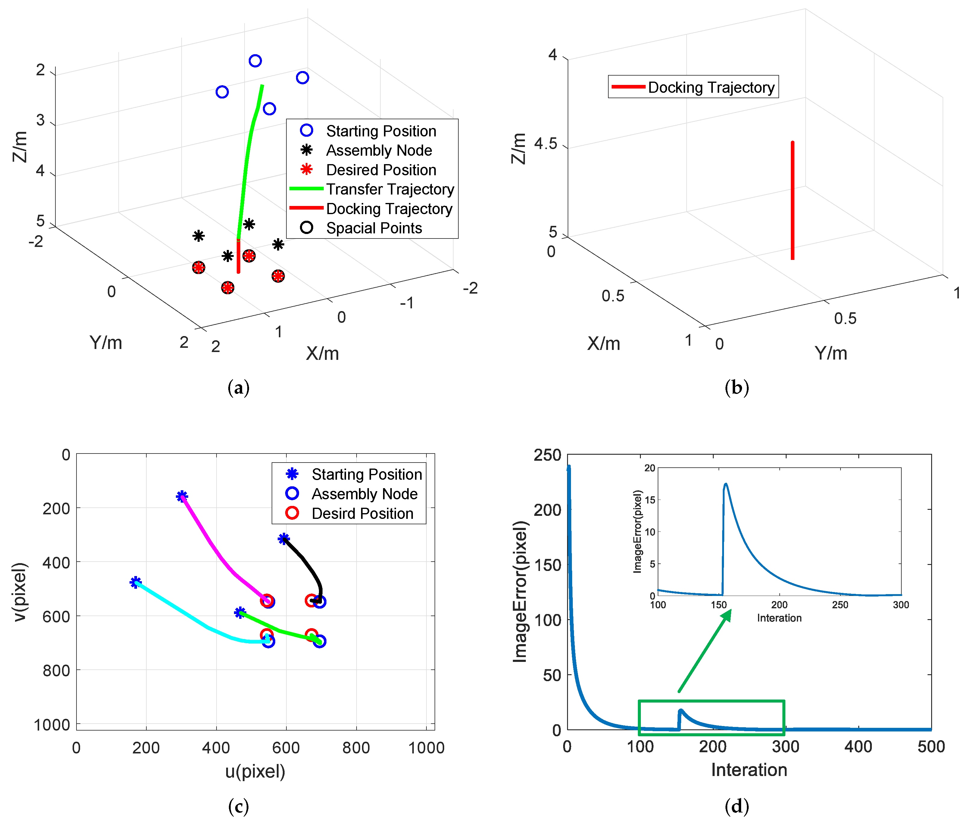
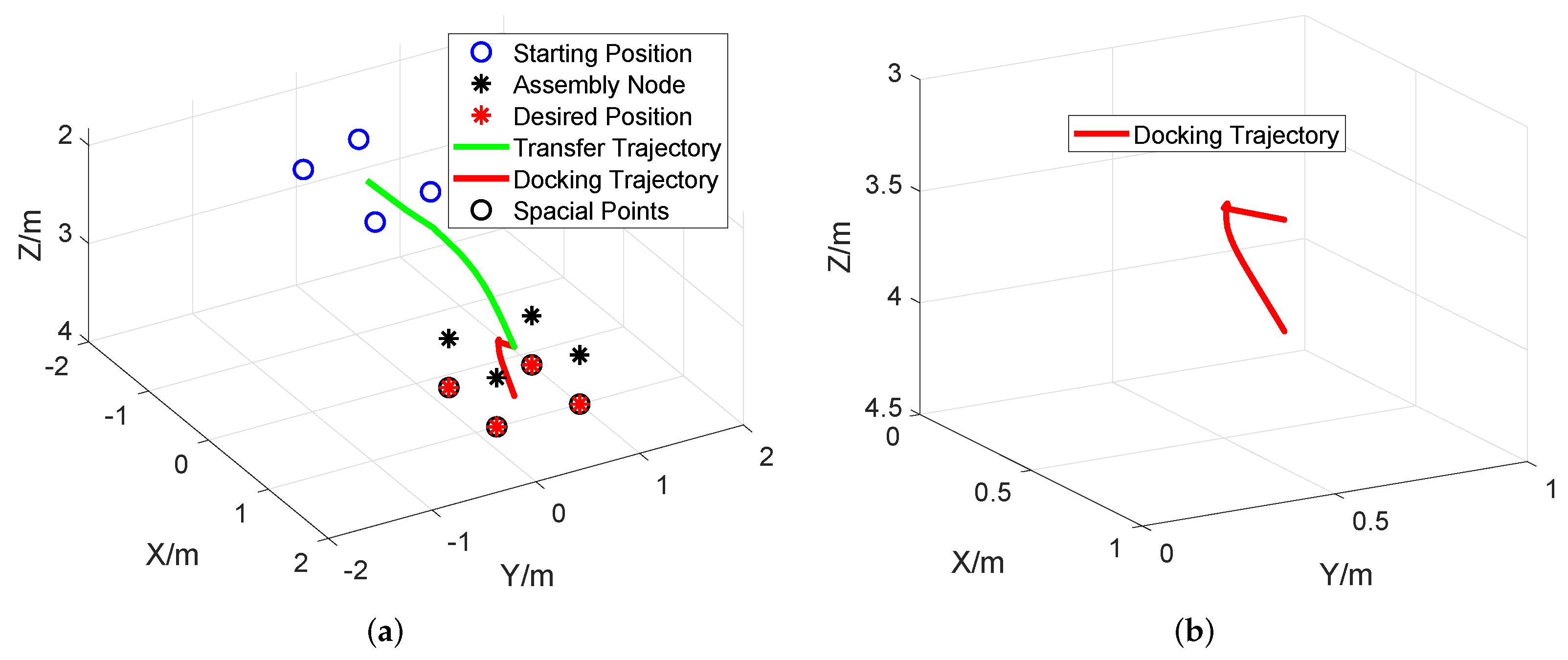
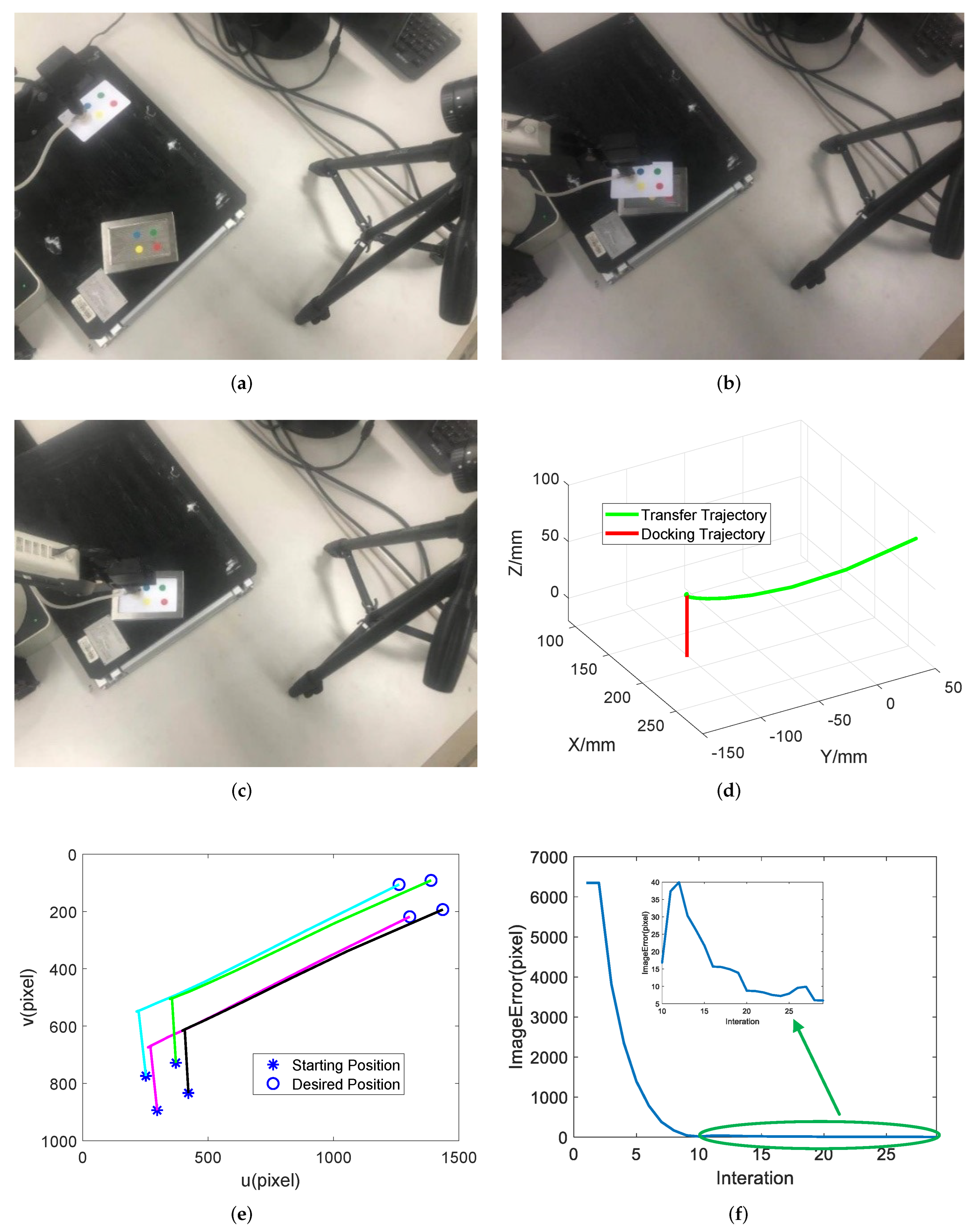
3.4. Docking Trajectory Planning
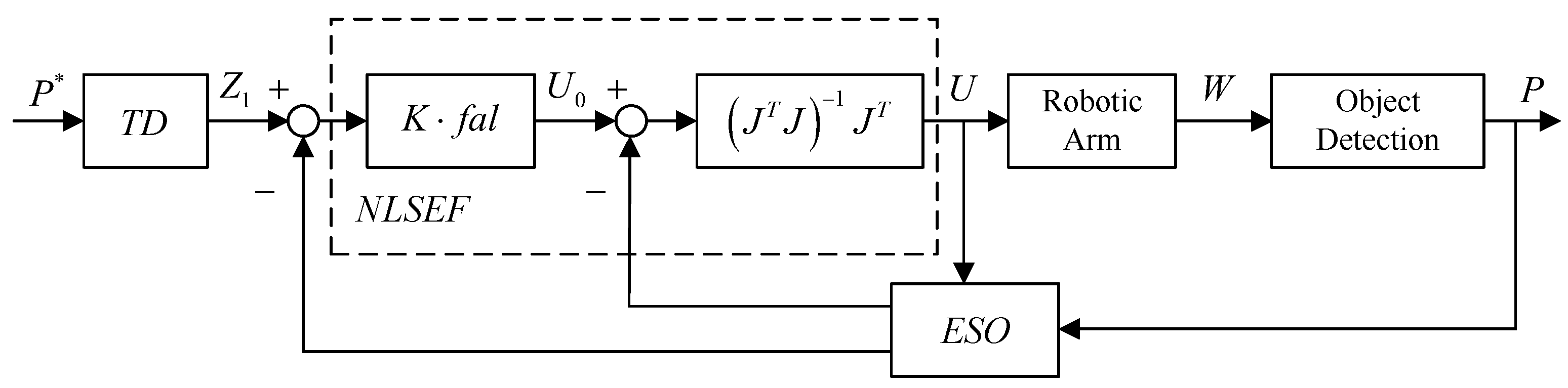
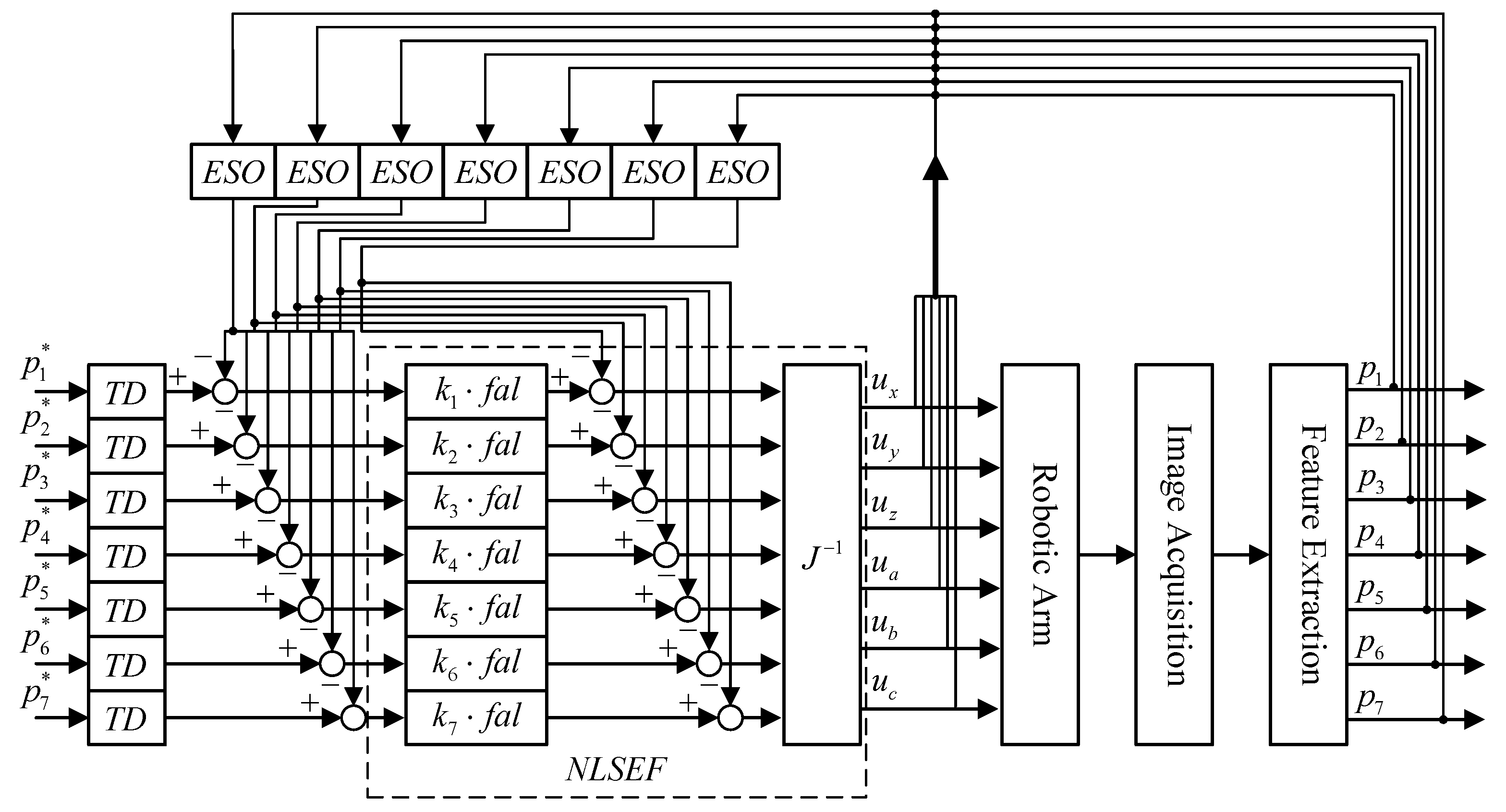
4. Design of Visual Servoing Controller Based on ADRC
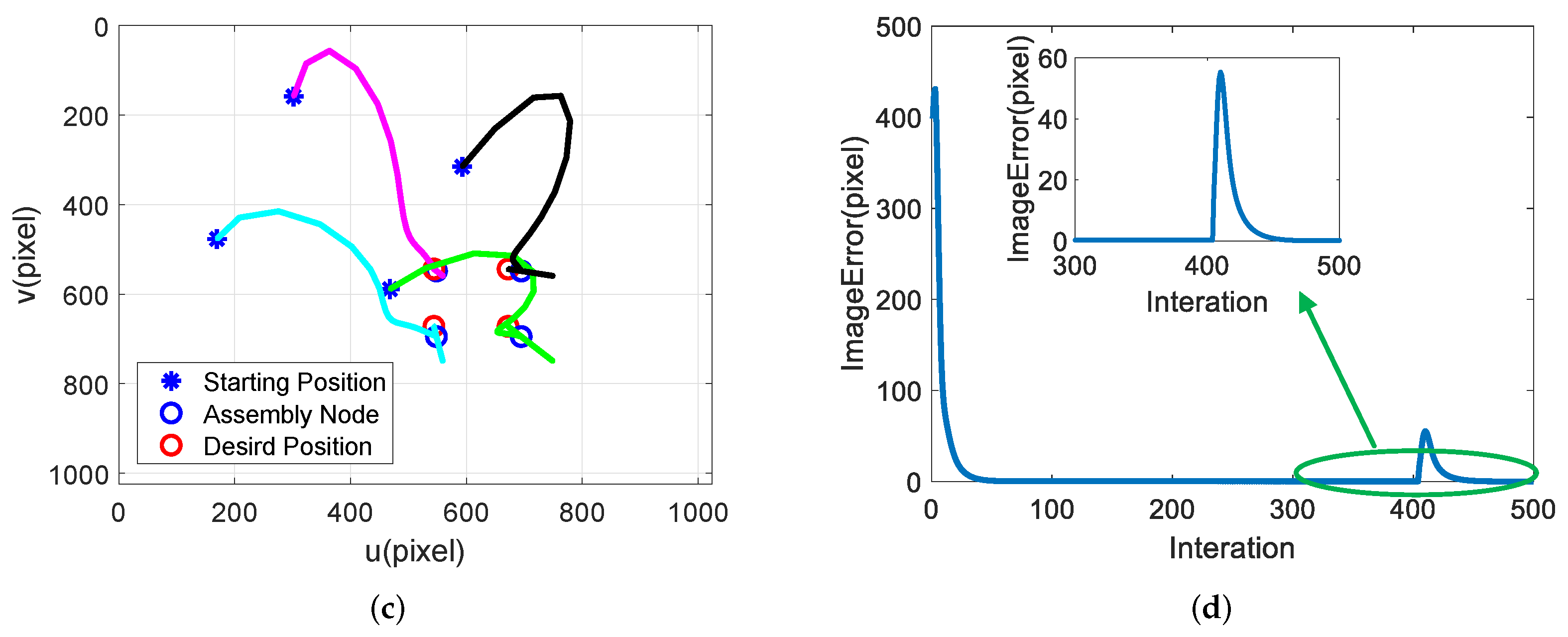
4.1. Image Features Selection
4.2. Controller Design
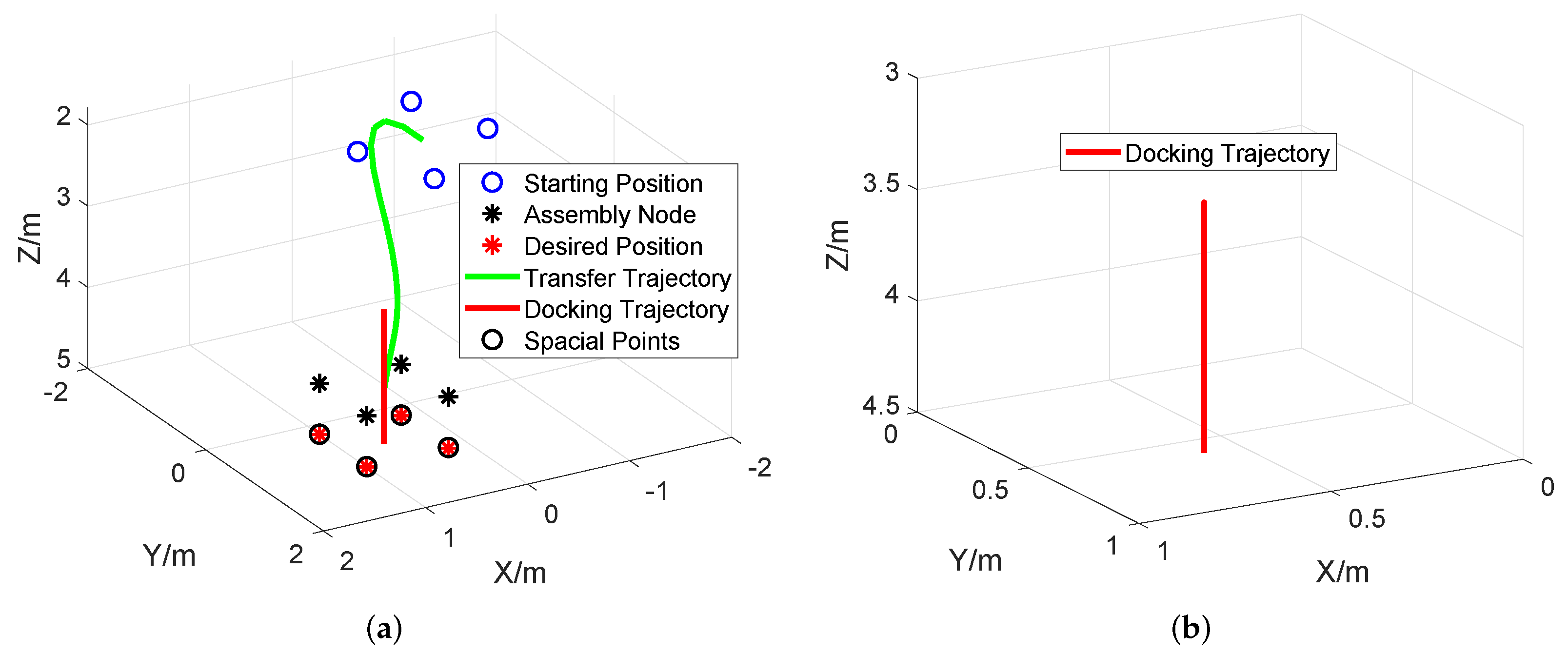
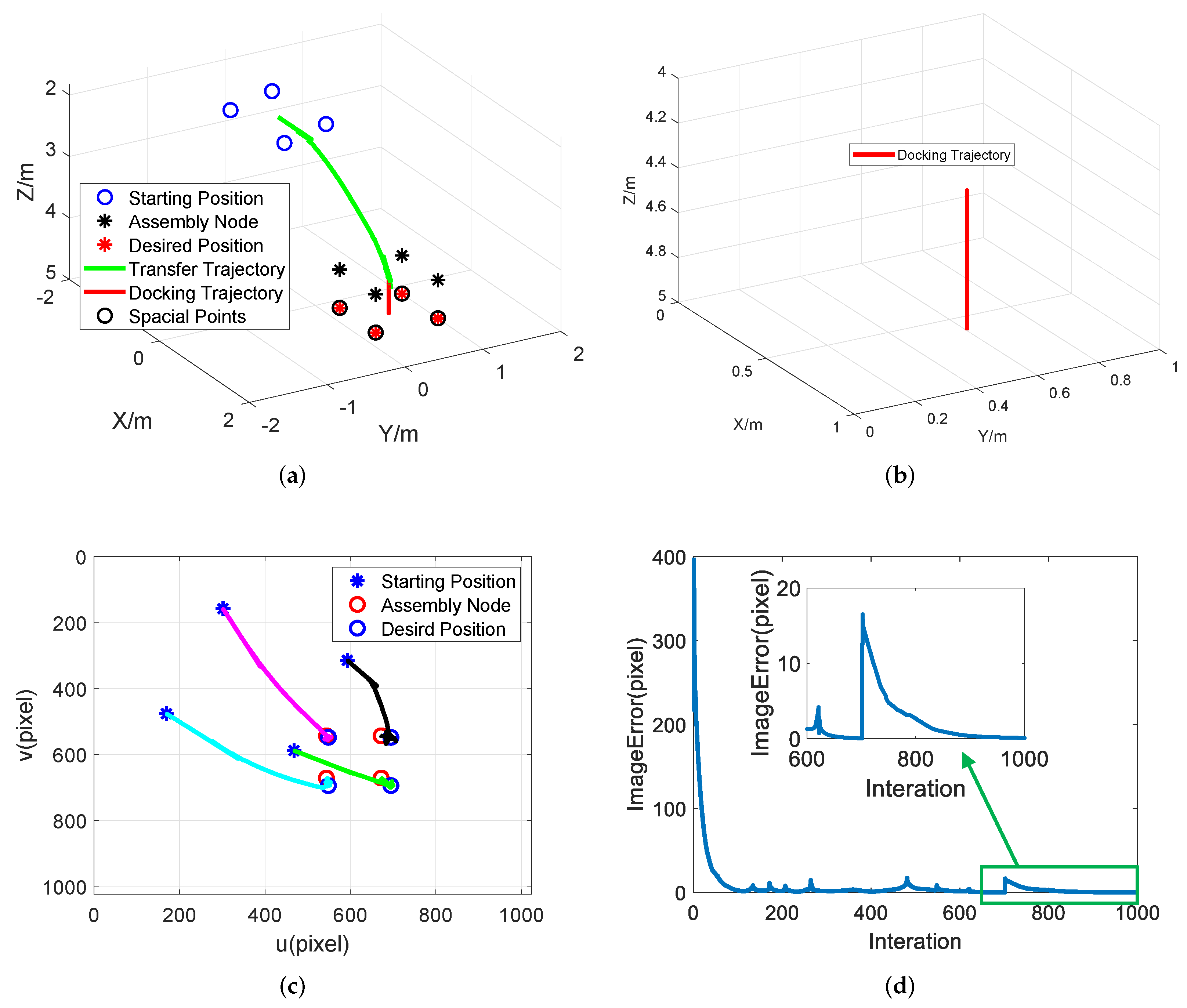
5. Simulation
5.1. Simulation Parameters
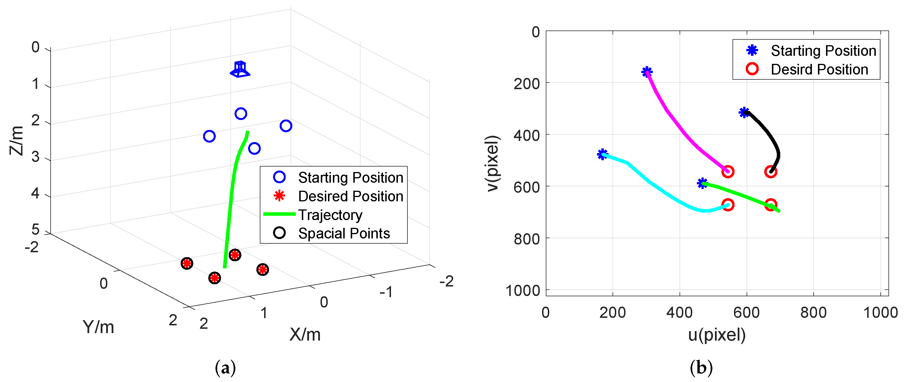
5.2. Simulation and Discussion
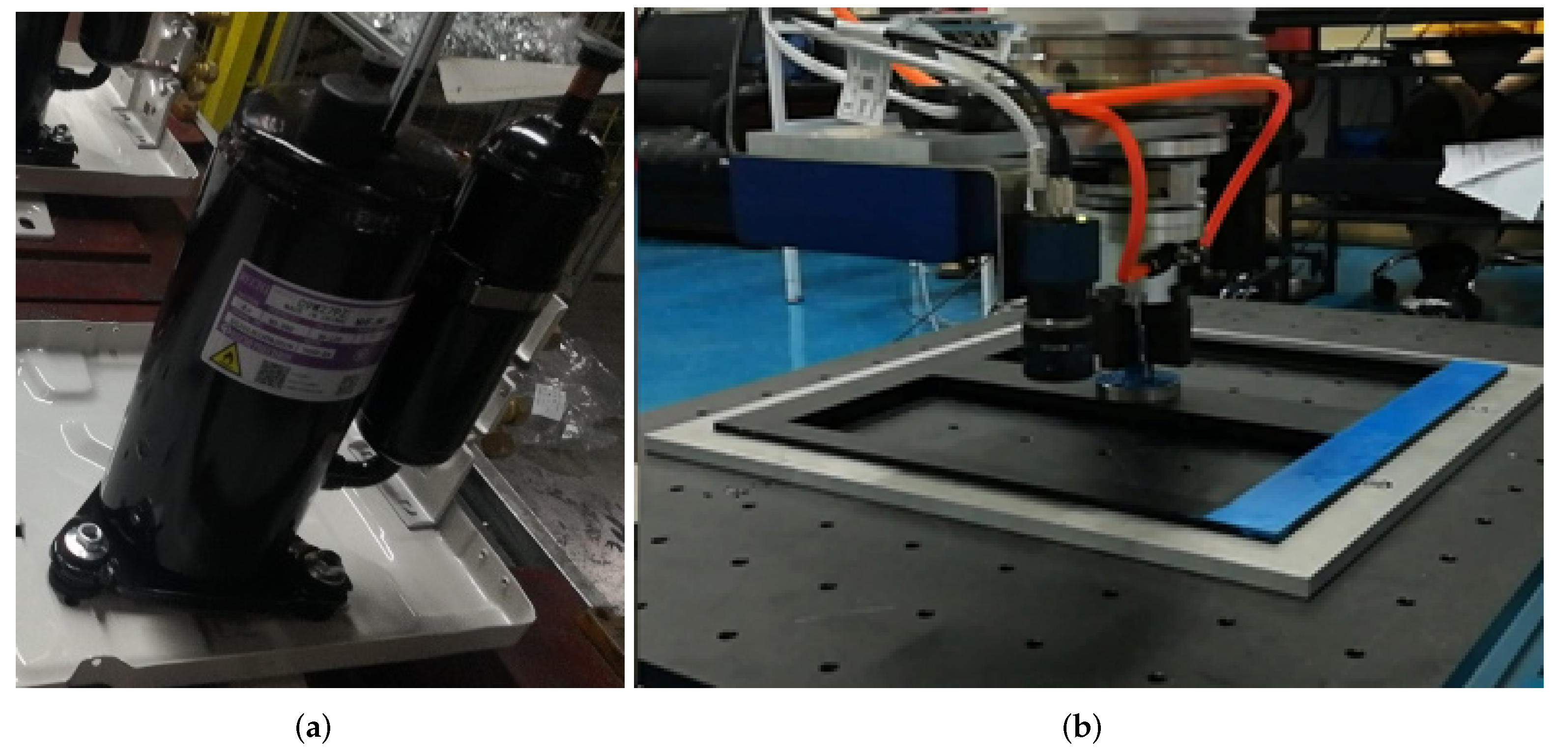
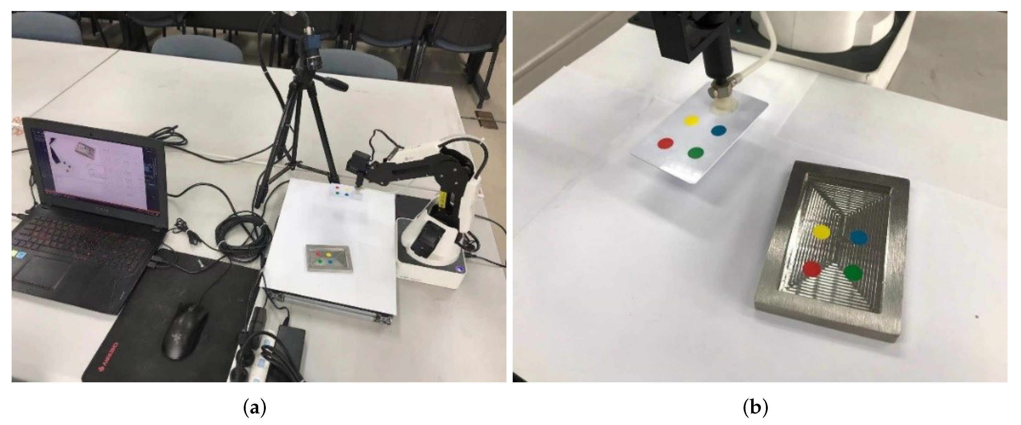
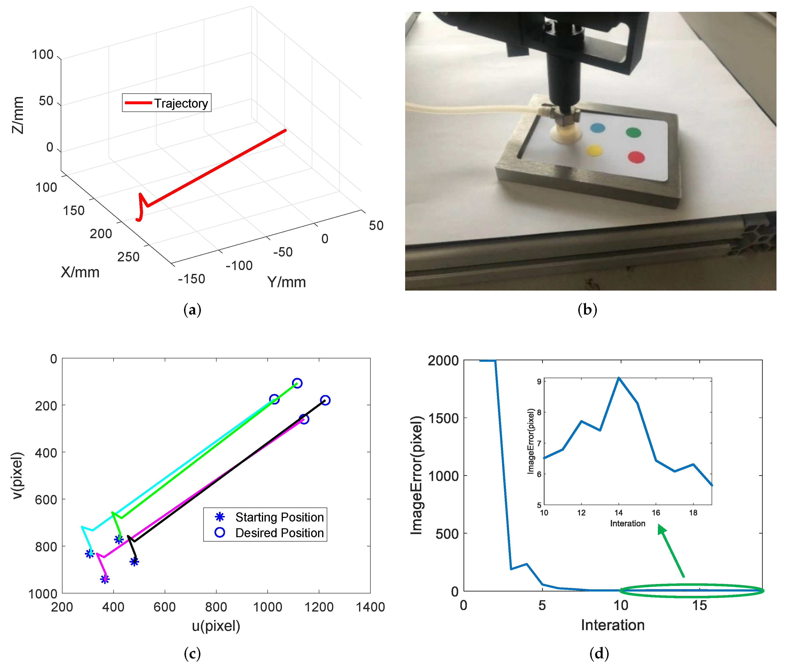
6. Experiment and Discussion
7. Conclusions
Funding
Data Availability Statement
Conflicts of Interest
References
- Hutchinson, S.; Chaumette, F. Visual servo control, Part I: Basic approaches. IEEE Robot. Autom. Mag. 2006, 13, 82–90. [Google Scholar]
- Bateux, Q.; Marchand, E. Histograms-based visual servoing. IEEE Robot. Autom. Lett. 2017, 2, 80–87. [Google Scholar] [CrossRef]
- Marchand, E. Subspace-based visual servoing. IEEE Robot. Autom. Lett. 2019, 4, 2699–2706. [Google Scholar] [CrossRef]
- Cheah, C.C.; Hirano, M.; Kawamura, S.; Arimoto, S. Approximate Jacobian control for robots with uncertain kinematics and dynamics. IEEE Trans. Robot. Autom. 2003, 19, 692–702. [Google Scholar] [CrossRef]
- Ma, Z.; Su, J. Robust uncalibrated visual servoing control based on disturbance observer. ISA Trans. 2015, 59, 193–204. [Google Scholar] [CrossRef]
- Corke, P.I.; Hutchinson, S.A. A new partitioned approach to image-based visual servo control. IEEE Trans. Robot. Autom. 2001, 17, 507–515. [Google Scholar] [CrossRef]
- Iwatsuki, M.; Okiyama, N. A new formulation of visual servoing based on cylindrical coordinate system with shiftable origin. In Proceedings of the IEEE/RSJ International Conference on Intelligent Robots and Systems, Lausanne, Switzerland, 30 September–4 October 2002; pp. 354–359. [Google Scholar]
- Janabi-Sharifi, F.; Deng, L.; Wilson, W.J. Comparison of basic visual servoing methods. IEEE-ASME Trans. Mechatron. 2011, 16, 967–983. [Google Scholar] [CrossRef]
- Xu, D.; Lu, J.; Wang, P.; Zhang, Z.; Liang, Z. Partially decoupled image-based visual servoing using difierent sensitive features. IEEE Trans. Syst. Man Cybern. Syst. 2017, 47, 2233–2243. [Google Scholar] [CrossRef]
- Lazar, C.; Burlacu, A. Visual servoing of robot manipulators using model-based predictive control. In Proceedings of the 2009 7th IEEE International Conference on Industrial Informatics, Cardiff, UK, 23–26 June 2009; pp. 690–695. [Google Scholar]
- Allibert, G.; Courtial, E.; Chaumette, F. Predictive control for constrained image-based visual servoing. IEEE Trans. Robot. 2010, 26, 933–939. [Google Scholar] [CrossRef]
- Wang, T.T.; Xie, W.F.; Liu, G.D.; Zhao, Y.M. Quasi-min-max model predictive control for image-based visual servoing with tensor product model transformation. Asian J. Control 2015, 17, 402–416. [Google Scholar] [CrossRef]
- Qin, S.J.; Badgwell, T.A. A survey of industrial model predictive control technology. Control Eng. Pract. 2003, 11, 733–764. [Google Scholar] [CrossRef]
- Milman, R.; Davison, E.J. Evaluation of a new algorithm for model predictive control based on non-feasible search directions using premature termination. In Proceedings of the 42nd IEEE Conference on Decision and Control, Maui, HI, USA, 9–12 December 2003; pp. 2216–2221. [Google Scholar]
- Hajiloo, A.; Keshmiri, M.; Xie, W.F.; Wang, T.T. Robust On-Line Model Predictive Control for a Constrained Image Based Visual Servoing. IRE Trans. Ind. Electron. 2016, 63, 2242–2250. [Google Scholar] [CrossRef]
- Besselmann, T.; Lofberg, J.; Morari, M. Explicit MPC for LPV systems: Stability and optimality. IEEE Trans. Autom. Control 2012, 57, 2322–2332. [Google Scholar] [CrossRef]
- Lofberg, J. YALMIP: A toolbox for modeling and optimization in MATLAB. In Proceedings of the 2004 IEEE International Symposium on Computer-Aided Control System Design, Taipei, Taiwan, 2–4 September 2004; pp. 284–289. [Google Scholar]
- Besselmann, T.; Lofberg, J.; Morari, M. Explicit model predictive control for linear parameter-varying systems. In Proceedings of the 47th IEEE Conference on Decision and Control, Cancun, Mexico, 9–11 December 2008; pp. 3848–3853. [Google Scholar]
- LaValle, S.M.; González-Banos, H.H.; Becker, C.; Latombe, J.C. Motion strategies for maintaining visibility of a moving target. In Proceedings of the IEEE International Conference on Robotics and Automation, Albuquerque, NM, USA, 25 April 1997; pp. 731–736. [Google Scholar]
- Gans, N.R.; Hutchinson, S.A.; Corke, P.I. Performance tests for visual servo control systems, with application to partitioned approaches to visual servo control. Int. J. Robot. Res. 2003, 22, 955–984. [Google Scholar] [CrossRef]
- Chesi, G.; Hashimoto, K.; Prattichizzo, D.; Vicino, A. Keeping features in the field of view in eye-in-hand visual servoing: A switching approach. IEEE Trans. Robot. Autom. 2004, 20, 908–914. [Google Scholar] [CrossRef]
- Mezouar, Y.; Chaumette, F. Path planning for robust imagebased control. IEEE Trans. Robot. Autom. 2002, 18, 534–549. [Google Scholar] [CrossRef]
- Hosoda, K.; Sakamoto, K.; Asada, M. Trajectory generation for obstacle avoidance of uncalibrated stereo visual servoing without 3D reconstruction. In Proceedings of the 1995 IEEE/RSJ International Conference on Intelligent Robots and Systems—Human Robot Interaction and Cooperative Robots, Pittsburgh, PA, USA, 5–9 August 1995; pp. 29–34. [Google Scholar]
- Hartley, R.; Zisserman, A. Multiple View Geometry in Computer Vision; Cambridge University Press: Cambridge, UK, 2003; pp. 1865–1872. [Google Scholar]
- Gonçalves, P.S.; Mendonça, L.F.; Sousa, J.M.C.; Pinto, J.C. Uncalibrated eye-to-hand visual servoing using inverse fuzzy models. IEEE Trans. Fuzzy Ssyt. 2008, 16, 341–353. [Google Scholar] [CrossRef]
- Khatib, O. Real-time obstacle avoidance for manipulators and mobile robots. Int. J. Robot. Res. 1986, 5, 90–98. [Google Scholar] [CrossRef]
- Kirkpatrick, S.; Gelatt, C.D., Jr.; Vecchi, M.P. Optimization by simulated annealing. Science 1983, 220, 606–615. [Google Scholar] [CrossRef]
- Sharma, R.; Sutanto, H. A framework for robot motion planning with sensor constraints. IEEE Trans. Robot. Autom. 1997, 13, 61–73. [Google Scholar] [CrossRef]
- Chesi, G. Straight line path-planning in visual servoing. J. Dyn. Syst. Meas. Control 2007, 129, 541–543. [Google Scholar] [CrossRef]
- Chesi, G. Visual servoing path planning via homogeneous forms and LMI optimizations. IEEE Trans. Robot. 2009, 25, 281–291. [Google Scholar] [CrossRef]
- Keshmiri, M.; Xie, W.F. Image-based visual servoing using an optimized trajectory planning technique. IEEE /ASME Trans. Mechatron. 2017, 22, 359–370. [Google Scholar] [CrossRef]
- Han, J. From PID to active disturbance rejection control. IEEE Trans. Ind. Electron. 2009, 56, 900–906. [Google Scholar] [CrossRef]
- Su, J.B. Robotic uncalibrated visual serving based on ADRC. Control Decis. 2015, 30, 1–8. [Google Scholar]
- Huang, Y.; Xue, W. Active disturbance rejection control: Methodology and theoretical analysis. ISA Trans. 2014, 53, 963–976. [Google Scholar] [CrossRef]


| Parameter | Value |
|---|---|
| Focal length | 0.008 |
| Length | 1024 |
| Width | 1024 |
| Coordinates of the projection center | (512,512) |
| Scaling factors | (0.00001,0.00001) |
| Part | Parameters | Value |
|---|---|---|
| TD | h | 0.1 |
| 0.02 | ||
| 0.12 | ||
| ESO | 0.5 | |
| 0.5 | ||
| 0.01 | ||
| 60 | ||
| 1200 | ||
| 15 | ||
| 0.7 | ||
| NLSEF | 0.5 | |
| 10.5 |
| Position | Num | Spatial Point | Image Point |
|---|---|---|---|
| Starting Position | 1 | (−0.48,−0.81,1.83) | (301.82,158.65) |
| 2 | (−0.81,−0.08,1.89) | (169.46,476.81) | |
| 3 | (−0.12,0.21,2.17) | (468.07,588.85) | |
| 4 | (0.21,−0.52,2.11) | (592.84,315.47) | |
| Desired Position | 1 | (0.2,0.2,5) | (544,544) |
| 2 | (0.2,1,5) | (544,672) | |
| 3 | (1,1,5) | (672,672) | |
| 4 | (1,0.2,5) | (689.24,544) |
| Terms | The Proposed Method | Conventional IBVS Method |
|---|---|---|
| Total Times | 50 | 50 |
| Successful Times | 50 | 0 |
| Average Error | < | |
| Time Consumption | > |
Publisher’s Note: MDPI stays neutral with regard to jurisdictional claims in published maps and institutional affiliations. |
© 2022 by the author. Licensee MDPI, Basel, Switzerland. This article is an open access article distributed under the terms and conditions of the Creative Commons Attribution (CC BY) license (https://creativecommons.org/licenses/by/4.0/).
Share and Cite
Cao, C. Research on a Visual Servoing Control Method Based on Perspective Transformation under Spatial Constraint. Machines 2022, 10, 1090. https://doi.org/10.3390/machines10111090
Cao C. Research on a Visual Servoing Control Method Based on Perspective Transformation under Spatial Constraint. Machines. 2022; 10(11):1090. https://doi.org/10.3390/machines10111090
Chicago/Turabian StyleCao, Chenguang. 2022. "Research on a Visual Servoing Control Method Based on Perspective Transformation under Spatial Constraint" Machines 10, no. 11: 1090. https://doi.org/10.3390/machines10111090
APA StyleCao, C. (2022). Research on a Visual Servoing Control Method Based on Perspective Transformation under Spatial Constraint. Machines, 10(11), 1090. https://doi.org/10.3390/machines10111090