A Fast Globally Convergent Particle Swarm Optimization for Defect Profile Inversion Using MFL Detector

Abstract

For the problem of defect inversion in magnetic flux leakage technology, a fast, globally convergent particle swarm optimization algorithm based on the finite-element forward model is introduced as an inverse iterative algorithm in this paper. Two aspects of the traditional particle swarm optimization algorithm have been improved: self-adaptive inertia weight and speed updating strategy. For the inertia weight, it can be adaptively adjusted according to the particle position. The speed update strategy mainly uses the best experience positions of other particles in a randomly selected population to realize the algorithm’s learning. At the same time, the learning factor of the position variable is designed to change with the number of iteration steps. The particle with a good position is added to jump out of the local minimum and accelerate the optimization process. Through the comparison experiment, the improved particle swarm optimization algorithm has a faster convergence speed compared with other traditional particle swarm optimization algorithms. It is more difficult for it to fall into the local minimum value and it is more easily converted to a higher precision.

1. Introduction

Magnetic flux leakage (MFL) detection technology is widely used to detect defects in oil pipelines [1]. Its main principle is to use a permanent magnet to magnetize the pipeline to saturation. If there is a defect in the pipe, the path of the magnetic induction lines at the defect will be changed, and a leakage magnetic field will be formed on the surface of the pipe [2]. By using Hall sensors to detect the leakage signal, the defect profile that generated the signal can be calculated. The process of estimating the defect profile according to the magnitude of magnetic leakage field is called the inversion process of the magnetic leakage detection [3].

Defect profile estimation based on magnetic flux leakage detection is a reverse process with some discomfort. The inversion method can be divided into two main categories. One is the direct, data-driven method (model-free) [4,5], and the other is the model-based indirect method (model-based) [6,7]. The direct method works by directly establishing a mapping relationship between the parameters of magnetic flux leakage signals and defect [8,9]. This relationship is then used to calculate the defect shape corresponding to the leakage signal [10]. Although this method has the advantage of being quick and easy, the generalization ability of the model is lower because the mapping parameters are based on the training sample. When the features of the actual defects are very different from those in the training samples, the accuracy of the defect size calculated by the quantitative model will be low. Most of the defects in practical applications are irregular, and these irregular defects will further affect the quantization accuracy of the inversion algorithm.

Therefore, more defect inversion methods are adopted based on models, which can not only realize the inversion of irregular defect profiles but also ensure high convergence accuracy. Model-based inversion methods usually include a forward model and an inverse algorithm [11]. The computational efficiency and accuracy of model-based inversion methods mainly depend on the following two factors: one is the degree of agreement between the forward model and the actual physical process [12], and the other is the stability, accuracy, and convergence speed of the optimization algorithm [13]. At present, the most widely used reverse algorithms include the gradient descent algorithm [14], the genetic algorithm [13,15], the particle swarm optimization algorithm [16,17], etc. These methods have their limitations and shortcomings. Gradient descent methods can easily converge to the local minimum value but cannot achieve high convergence accuracy. For premature convergence in multimodal search problems, genetic algorithms and PSO algorithms exist. Early diversity groups are more likely to lose diversity and fall into local minima, and the search speed is slower.

Therefore, this paper improved the basic particle swarm optimization (BPSO) algorithm and proposed a fast, globally convergent, particle swarm optimization algorithm. This algorithm can effectively improve the speed and accuracy of defect inversion. The main contributions of this paper are as follows:

• A traditional particle swarm optimization algorithm cannot match the appropriate motion state for each particle. This paper introduces the concept of personalized inertia weight. This method judges the current position of each particle by comparing the fitness of each particle with the average fitness of the population. Based on the state, the inertia weight of particles with a better position is reduced, and the particles are focused on the development of the current region. For the particles in poor position, the inertia weight of the particle is increased, causing the particle to focus on potential area exploration. Compared with the BPSO algorithm, this method has been proven to have a faster convergence speed.
• The particle swarm optimization algorithm easily falls into a local minimum in the process of inversion iteration. This paper proposes a new speed update strategy. By introducing the optimal experiential positions of other random particles in the population to learn, this strategy causes the experiential learning object of the particle group to change from the original single object to multiple objects. This method has a learning factor that linearly decreases with the number of iteration steps, which makes the algorithm improve the population diversity in the early stage and avoids the algorithm instability caused b” ran’omness in the later stage.
• Experimental verification shows that the proposed algorithm achieves higher convergence accuracy and faster convergence speed compared with existing methods, such as particle swarm optimization and gradient descent.

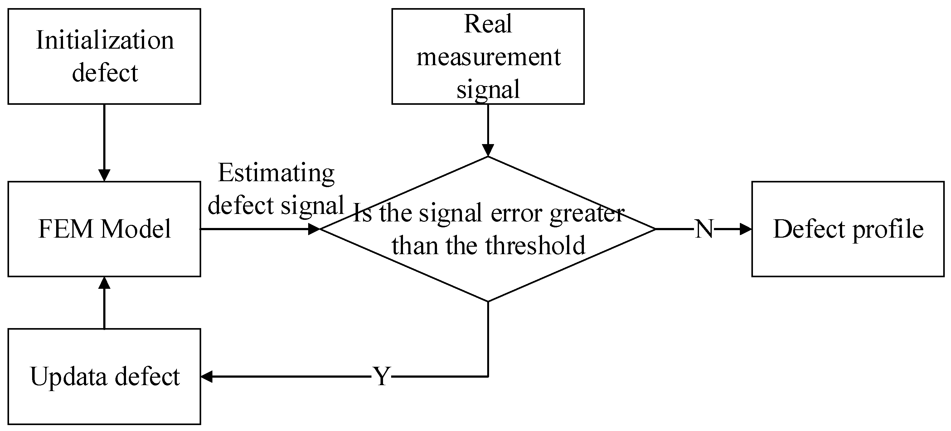
2. Inversion Process of Irregular Defects

2.1. Defect Inversion Process

The reverse process of the defect profile is shown in Figure 1. Firstly, initialize a defect profile $s$, and then use the forward model to calculate the magnetic leakage signal of the defect $B(s)$. Secondly, compare the simulation signal $B(s)$ with the signal $B(s_{real})$ collected by the actual sensor to obtain the error $E={\displaystyle \sum {\left(B(s)-B(s_{real})\right)}^2}$ of the convergence target. Thirdly, using the optimization algorithm, the next iteration profile $s^{\prime }$ can be calculated based on the error $E$ of the convergence target. Fourth, repeat the above process until the error of the convergence target is less than the set threshold, and the iteration process is completed. Generally, the setting of the termination threshold condition can be determined according to the error between simulated signal and measured signal. The error is calculated by the profiles of some known defect samples. The profile obtained at this time is considered to be the profile $s_{real}$ that is closest to the real defect.

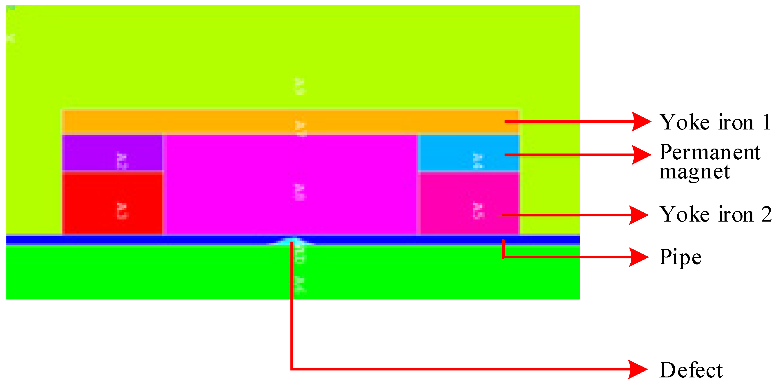
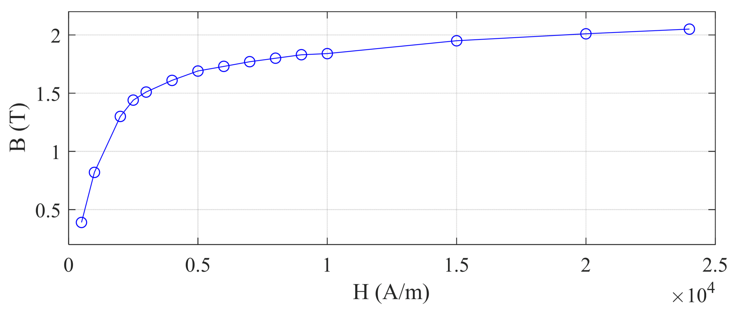
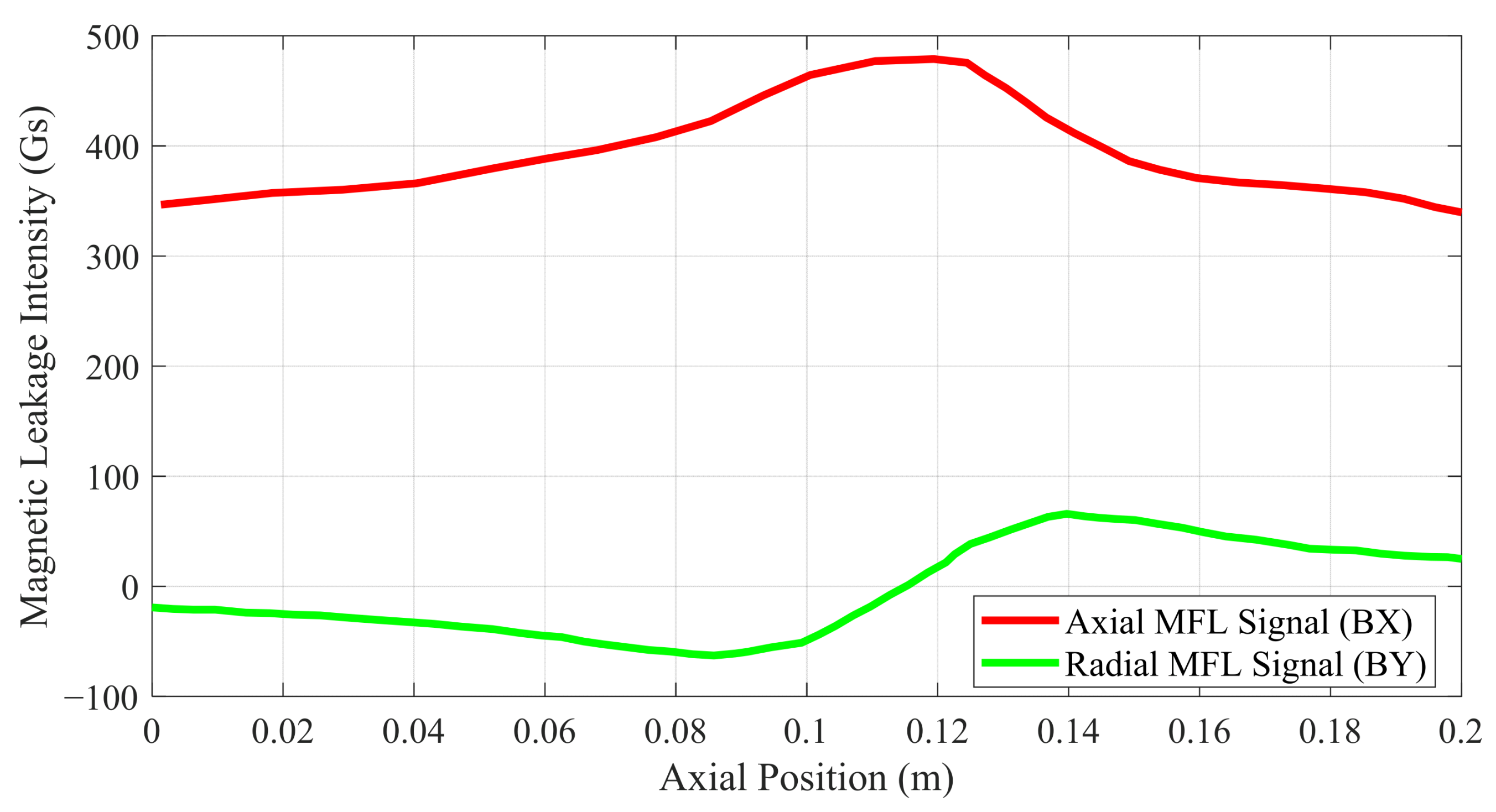
2.2. Forward Finite-Element Modeling

In this paper, the software ANSYS 19.0, based on the method of finite-element analysis, is adopted to build and solve the simulation forward model of the defect MFL. In order to ensure a degree of agreement between the FEM model and the actual physical process, it is necessary to ensure that the parameters (such as permeability, model size, coercive force, etc.) of each element (such as permanent magnet, yoke iron, pipe wall, etc.) in the simulation model are the same as or similar to the parameters of the actual detector. The structure and material properties of the model are shown in Figure 2 and Figure 3 and Table 1.

Table 1. Properties of the finite-element simulation model.

Components	Materials	Coercive Force (Unit: KA/m)	Relative Permeability (Unit: 1)	Length (Unit: mm)	Height (Unit: mm)
Yoke Iron 1	Iron DT4C	-	5 × 10³	360	20
Permanent Magnet	Neodymium 45	8.76 × 10²	1	80	30
Yoke Iron 2	Iron DT4C	-	5 × 10³	80	30
Pipe	Steel X45	-	BH curve in Figure 3	460	8
Defect	Air	-	1	40	7.5

Table 1. Properties of the finite-element simulation model.

Components	Materials	Coercive Force (Unit: KA/m)	Relative Permeability (Unit: 1)	Length (Unit: mm)	Height (Unit: mm)
Yoke Iron 1	Iron DT4C	-	5 × 10³	360	20
Permanent Magnet	Neodymium 45	8.76 × 10²	1	80	30
Yoke Iron 2	Iron DT4C	-	5 × 10³	80	30
Pipe	Steel X45	-	BH curve in Figure 3	460	8
Defect	Air	-	1	40	7.5

The opening profile of the defect is determined by depth values of the defect along the path on the inversion section. The depth values on this path can have a variety of combination results according to the number of degrees of freedom. This can be represented by a vector s.

$$s=\left[s_1,s_2,\dots ,s_m\right]$$

(1)

where $m$ represents the number of freedom degrees, and $s_i$ represents the defect depth value corresponding to the position of the $i^{th}$ freedom degree.

After the forward model in Figure 2 is meshed into grids, the ANSYS software solves the electromagnetic field differential equation of each grid. The calculated magnetic flux leakage signals are shown in Figure 4. BX and BY represent the radial and axial magnetic signals of the defect, respectively. Since the structure of the detector is axisymmetric when it runs in the pipeline, a two-dimensional simulation model on a section is selected in this paper to simulate the three-dimensional actual physical process.

3. FGC-PSO Algorithm for Defect Inversion

In order to realize the iteration process of the above defect profile inversion, it is very important to calculate the next iteration defect profile $s^{\prime }$ by using the error between the simulated signal and the real signal. Using a good optimization method can more efficiently produce a more accurate defect profile. The commonly used optimization methods include gradient descent, genetic algorithms, particle swarm optimization, and so on. This paper improves the traditional particle swarm optimization algorithm and designs a novel method that is more suitable for defect profile inversion processes, called the fast globally convergent particle swarm optimization algorithm (FGC-PSO).

3.1. Basic Particle Swarm Optimization Algorithm

The particle swarm optimization algorithm (PSO) carries out a parallel random search on the optimization space by simulating the process of bird foraging to seek the optimal solution, and the existence state of each particle in the PSO is described by two aspects: particle position and motion speed. Each particle’s position information is seen as a potential solution of space. At the same time, using the optimization goal set by the fitness function ${\phi }_i=f\left(x_i\right)$ as the standard, the merits of each potential solution to each particle are judged according to the evaluation results. The speed is updated by self and social learning with its own optimal experience position and the particle swarm’s optimal experience position. After the update, the position of the particles will change, and then the particles will be further searched in the new optimization domain. The optimal empirical position of each particle and particle swarm will also change with the new search. This evolutionary process will be repeated continuously until the particle swarm finds a solution that meets the requirements, or the evolutionary algebra reaches the upper limit. Finally, the optimal solution obtained by the population will be output as the optimization result. The evolutionary rules of the particle swarm optimization algorithm are as follows:

$$v_i^{t+1}={\omega }_i^t{v}_i^t+c_1{r}_1(pbes{t}_i^t-x_i^t)+c_2{r}_2(gbes{t}_i^t-x_i^t)$$

(2)

$$x_i^{t+1}=x_i^t+v_i^{t+1}$$

(3)

where $x_i^t$ and $v_i^t$ represent the position and velocity of the $i^{th}$ particle in the $t^{th}$ iteration, respectively. $i=1,2,\dots ,j$ represents the number of particles in the particle swarm. $pbest$ represents the self-optimal experience position of each particle. $pbes{t}_i^t-x_i^t$ is a self-learning vector, and represents the search experience of the particle itself. $gbest$ represents the optimal experience position of the whole group. $gbes{t}_i^t-x_i^t$ is a social learning vector, and represents the search experience of the particle group. $c_1$ and $c_2$ represent the learning factors before the self-learning and the social-learning, respectively. $r_1$ and $r_2$ are uniformly distributed random numbers in the range of [0, 1].

${\omega }_{}^t$ is the inertial weight of the $t^{th}$ iteration, and represents the speed proportion between the $t^{th}$ and ${(t+1)}^{th}$ iterations of particles. In general, if the inertia weight increases, the global search capability of the algorithm will become stronger, and the optimal experience position in the group will be less affected. The inertia weight in the basic particle group algorithm linearly decreases with iterations.

$$\omega (t)={\omega }_{\max }-\left({\omega }_{\max }-{\omega }_{\min }\right)\times \frac{t}{ Iter }$$

(4)

where ${\omega }_{\max }$ represents the maximum inertia weight of the particle swarm, and is the initial inertia weight of the particle swarm. ${\omega }_{\min }$ represents the minimum inertia weight of the particle swarm. $Iter$ represents the maximum number of iterations of the particle swarm, and its value is related to the accuracy requirements.

3.2. Fast Globally Convergent Particle Swarm Optimization Algorithm

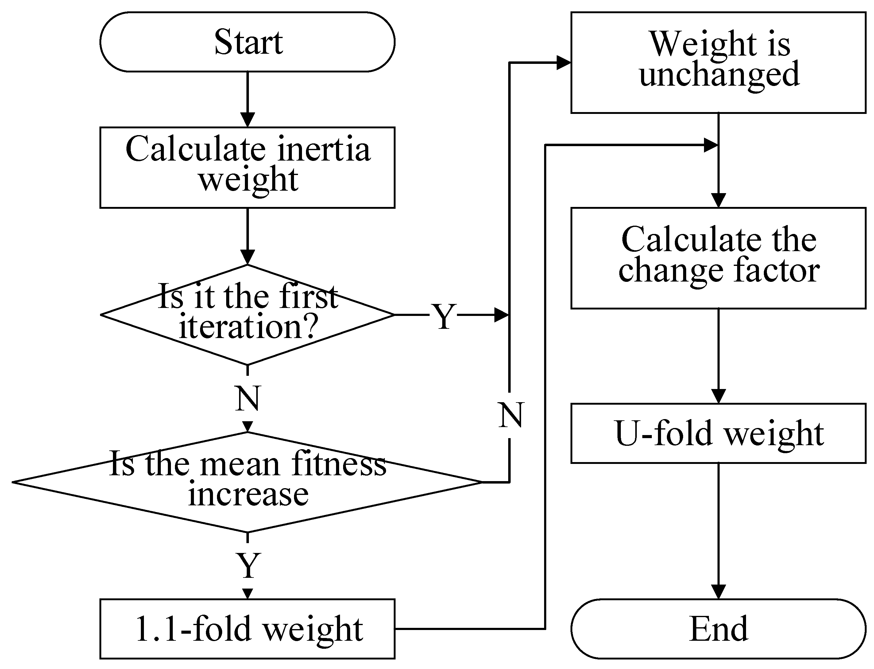
3.2.1. Self-Adaptive Inertia Weight

In PSO, inertia weight $\omega$ can greatly determine the search ability of the algorithm. A larger $\omega$ means that particles have a strong global search ability and weak local development ability, while a smaller $\omega$ means that particles have a strong local development ability and weak overall search ability.

In basic particle swarm optimization (BPSO), a linearly decreasing inertia weight can cause PSO have a higher global search ability in the early stage of evolution, which is conducive to fully exploring the potential optimal region of the solution space as much as possible. In the later stage of evolution, it has a higher local development ability, which is conducive to the development of the most potential optimization region to obtain the global optimal solution.

In the BPSO algorithm, all particles share the same inertia weight, $\omega$. The value of $\omega$ is only related to the number of iterations, $t$, and has nothing to do with the current motion state of particles. In the early stage of the algorithm, the larger inertia weight makes the particles with better positions unable to carry out fine local development, which may miss the global optimal solution of the current optimal region. However, in the later stage of the algorithm, the smaller inertia weight causes the particles with poor positions to stagnate in the local development of the surrounding poor area, which cannot contribute to the optimization of the population.

Therefore, based on the limitations of the BPSO algorithm, an improved inertia weight calculation method is proposed. On the basis of the original linearly decreasing inertia weight, the following two factors are introduced: firstly, the iterative process considers the changing trend in population fitness. If the mean value of population fitness increases, the overall position of the population becomes worse. At this time, the inertia weight of the particle swarm is increased as a whole. Secondly, the inertia weight change factor $u$ is introduced, which is related to the current motion state of the particle. If the fitness of the particle’s current position is lower than the average fitness of the group, is indicates that the current particle is in a better position in the group, and the change factor $u$ will play a role in reducing the inertia weight of the particle.

The specific calculation process of inertia weight is shown in Figure 5, and the steps are as follows.

Step 1: After the improvement, each particle of particle swarm has an independent inertia weight, which is expressed as $\omega =\left[{\omega }_1,{\omega }_2,\dots ,{\omega }_j\right]$. First, the inertia weight $\omega {(t)}_{BPSO}$ based on BPSO is calculated according to the Formula (4), and then $\omega {(t)}_{BPSO}$ is assigned to the inertia weight of each particle.

$${\omega }_i^t=\omega {(t)}_{BPSO},i=1,2,\dots ,j$$

(5)

Step 2: When the current iteration steps satisfy $t>1$, compare the mean $f_{aver}$ of population fitness in this iteration with the mean $f_{pre\_aver}$ of population fitness in the last iteration. If $f_{aver}<f_{pre\_aver}$, this means that the particle swarm is in a good position, and the inertia weight calculated in Step 1 does not need to be changed. If $f_{aver}>f_{pre\_aver}$, then the position of the whole particle swarm becomes worse. At this time, the inertia weight $\omega$ of all particles is increased by 1.1 times. If $f_{aver}<f_{pre\_aver}$, then ${\omega }_i^{t+1}={\omega }_i^t$. If $f_{aver}>f_{pre\_aver}$, then ${\omega }_i^{t+1}=1.1\times {\omega }_i^t$;

Step 3: The following inertia weight variation factors $u_i$ are introduced.

$$u_i=\frac{0.8}{\pi }\times \arctan \left(\frac{f\left(x_i\right)}{f_{aver}}-1\right)+1$$

(6)

The inertia weight obtained in Step 2 is multiplied by the inertia weight variation factor.

$${\omega }_i^{t+1}={\omega }_i^t\times u_i$$

(7)

when $f\left(x_i\right)>f_{aver}$, it shows that the particle has experienced a worse position than most of the particles in the group; then, the working center of the particle should be placed in the exploration of other potential better areas, which requires a strong global search ability. Therefore, the inertia weight needs to be increased. At this time, the corresponding $u$ is greater than 1, and the larger the $u$ corresponding to the particle with the worse position will be. When $f\left(x_i\right)<f_{aver}$, it shows that the particle has experienced a better position than most of the particles in the group, the working center of gravity of the particle should be more placed in the further development of the better position, and needs a strong local development ability. Therefore, the inertia weight needs to be reduced. At this time, $u$ is less than 1. The particle with better position has a smaller $u$ value.

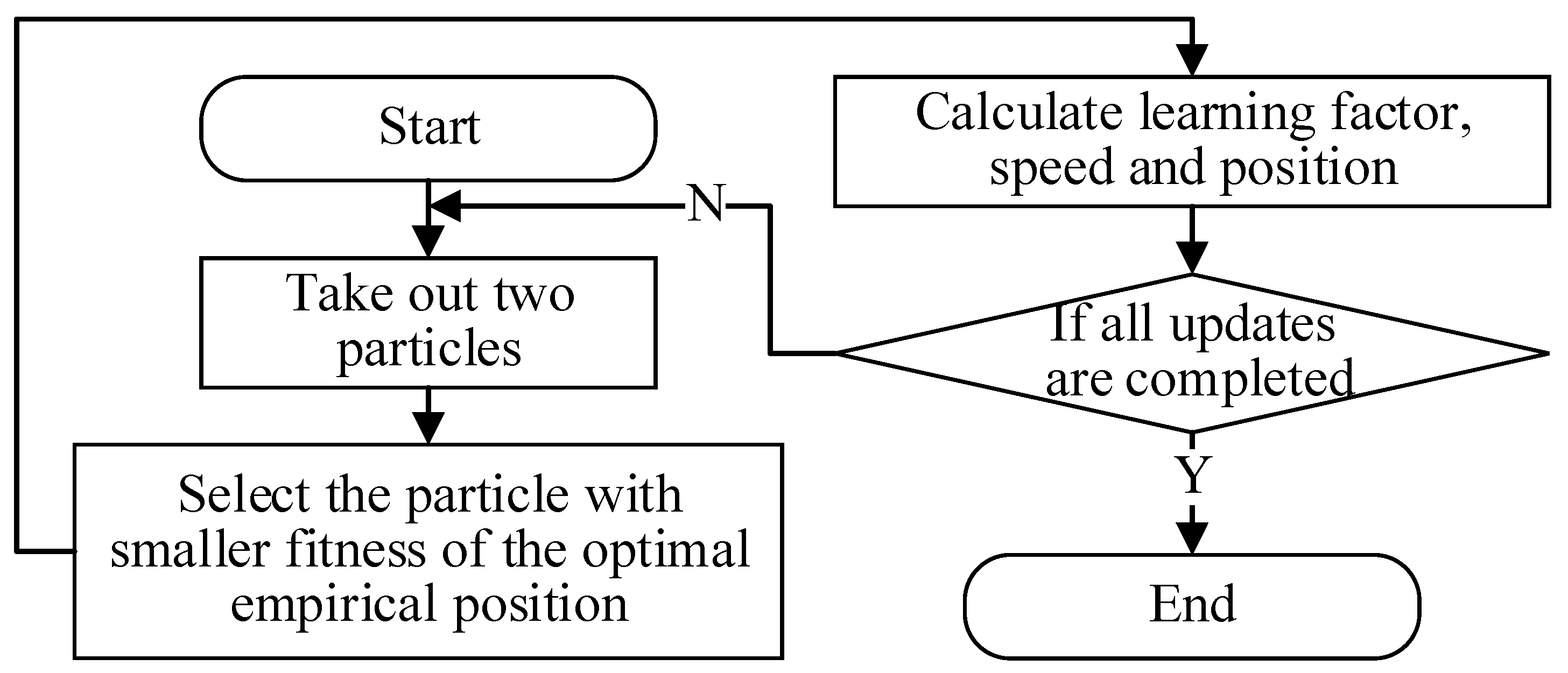
3.2.2. Improved Speed Updating Strategy

The speed update formula of the basic particle swarm optimization algorithm is shown in Equation (2). In this equation, the speed of this iteration of particle swarm optimization is determined by three factors: the first is the speed of the last iteration, which represents the inertia of particle motion. The second is the optimal position $pbes{t}_i$ of the particle’s own experience, which indicates that the particle learns from its own experience. The third is the optimal position experienced by the whole group, which represents the particle learning from the group experience. Among them, the learning of group experience by particles is only based on the optimal experience position $g_{best}$ of the group. No matter whether other particles in the group have made a full global exploration or not, the positions of all particles will be close to the optimal position of the single group $g_{best}$. From the perspective of short-term search behavior, the PSO can quickly approach the known optimal empirical position of the population and accelerate the convergence speed. However, from the perspective of long-term search behavior, it is easy to cause the particle swarm to lose the diversity of the population in the early stage and fall into the local minimum, resulting in slow convergence or even being unable to converge after falling into the local minimum. Due to the aforementioned drawbacks, this study presents the ideal empirical position $pbes{t}_c$ of other particles in the population to learn, based on the original velocity update equation. By giving the particles the ability to learn from their peers randomly, the population diversity is enhanced, and the particle swarm is prevented from falling into a local optimum.

$$\begin{array}{c}{v}_i^{t+1}={\omega }_i^t{v}_i^t+c_1{r}_1(pbes{t}_i^t-x_i^t)+c_2{r}_2(gbes{t}^t-x_i^t)\\ +c_3{r}_3(pbes{t}_c^t-x_i^t)\end{array}$$

(8)

In the above equation, $r_1$, $r_2$ and $r_3$ are random numbers tha tare uniformly distributed in the interval [0, 1], among which the selection process of $c$ with the optimal empirical position $pbes{t}_c$ is as follows:

Step 1: Randomly take two particles $a$ and $b$ out of a total of $j$ particles;

Step 2: Calculate the fitness $f\left({pbest}_a\right)$ and $f\left({pbest}_b\right)$ corresponding to the most experienced position of two particles;

Step 3: $c$ is the particle corresponding to the smaller fitness. If $f\left({pbest}_a\right)<f\left({pbest}_b\right)$, then $c=a$, otherwise, $c=b$.

After selecting particle $c$, $c_3$ is designed to linearly decrease according to the number of iteration steps. The change of $c_3$ follows Equation (9), where $c_{32}$ is the maximum of $c_3$ and $c_{31}$ is the minimum of $c_3$.

$$c_3=c_{32}-\left(c_{32}-c_{31}\right)\times \frac{t}{ Iter }$$

(9)

In the early stage of the algorithm, particle swarm optimization needs to improve the diversity of the population to enhance the global search ability of the population and avoid prematurely falling into local extremum. As a result, it is more important to introduce a certain rate of update randomness and divergence to other particles in order to increase particle position diversity. However, in the later stage of the algorithm, PSO focuses more on the fine local development of the better position, so it is necessary to appropriately weaken the learning of other particles to weaken the instability of the population movement, so as to facilitate the development of the current better position and find the optimal solution. The improved speed update process is shown in Figure 6.

3.3. Defect Inversion Process Base on FGC-PSO Algorithm

Using the forward model based on finite element and improved PSO algorithm mentioned above, the iterative inversion of complex defect profile can be realized. The specific defect inversion process is as follows:

Step 1: Collect the magnetic flux leakage signal $B(s_{real})$ of defects in the pipeline, and initialize a defect vector $s$. According to the defect vector, the forward model based on finite element method is constructed, and the magnetic flux leakage signal $B(s)$ of the forward model is solved.

Step 2: Initialize the particle swarm optimization and generate $j$ particles, which represent the estimated values of the profile parameters of the irregular pipeline defect, respectively. Each particle has a corresponding position vector $x_i=\left[x_{i1},x_{i2},\dots ,x_{im}\right]$ and velocity vector $v_i=\left[v_{i1},v_{i2},\dots ,v_{im}\right]$. Each freedom degree of $x_i$ and $v_i$ represents the percentage of the freedom degree of each defect in the thickness of the pipe.

Step 3: Calculate the inertia weight of each particle based on the improved inertia weight method. Each particle in the particle swarm has an independent inertia weight $\omega =\left[{\omega }_1,{\omega }_2,\dots ,{\omega }_j\right]$.

Step 4: Update the particle velocity $v_i$ and position $x_i$ based on the improved speed updating strategy.

Step 5: Input $j$ estimated defect profile parameters $x_i=\left[x_{i1},x_{i2},\dots ,x_{im}\right](i=1,2,\dots ,j)$ generated by particle swarm optimization algorithm into the forward model to obtain the magnetic flux leakage $B\left(x_i\right)$.

Step 6: Calculate the fitness $f\left(x_i\right)$ of each particle and calculate the average fitness of the population $f_{aver}$;

Step 7: Determine the group optimal empirical position ${gbest}^t$ of the particle swarm and the optimal empirical position ${pbest}^t$ of each particle in the $t^{th}$ iteration.

Step 8: Compare whether the fitness function corresponding to ${gbest}^t$ reaches the target accuracy. If so, the inversion process is finished. At this time, the updated profile parameters are the final inversion results. If not, skip to Step 3 for the next iteration;

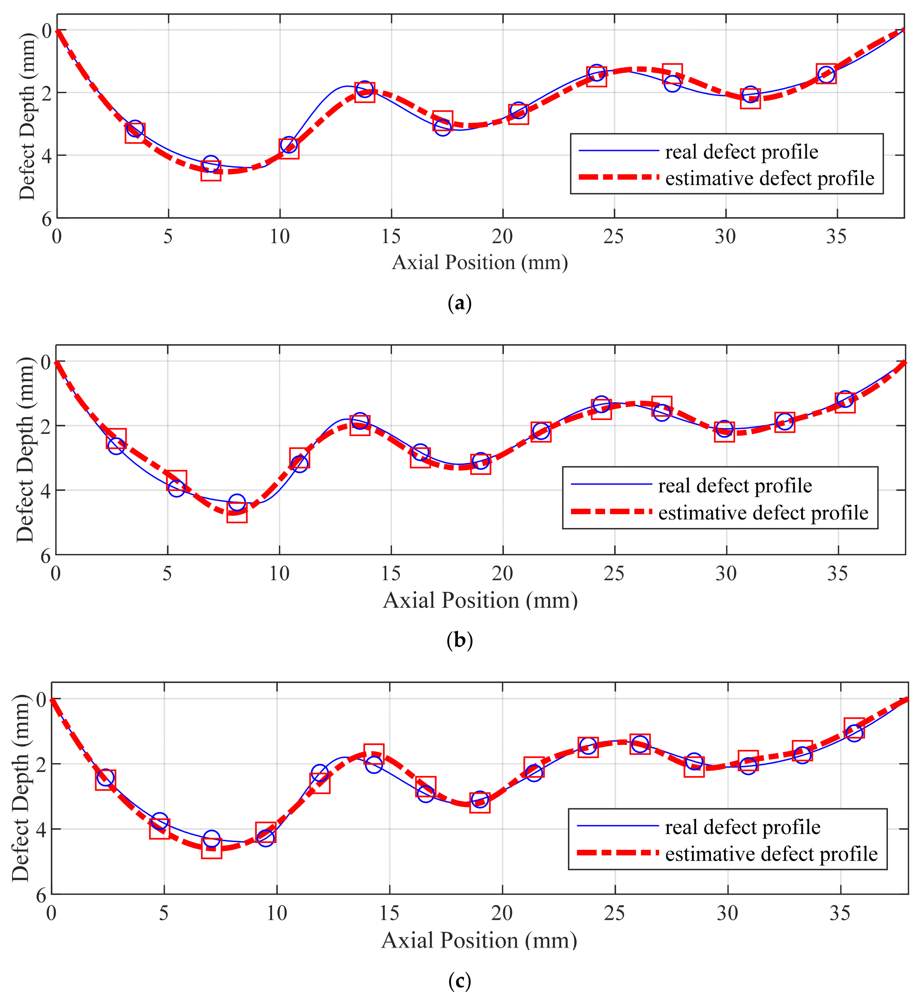
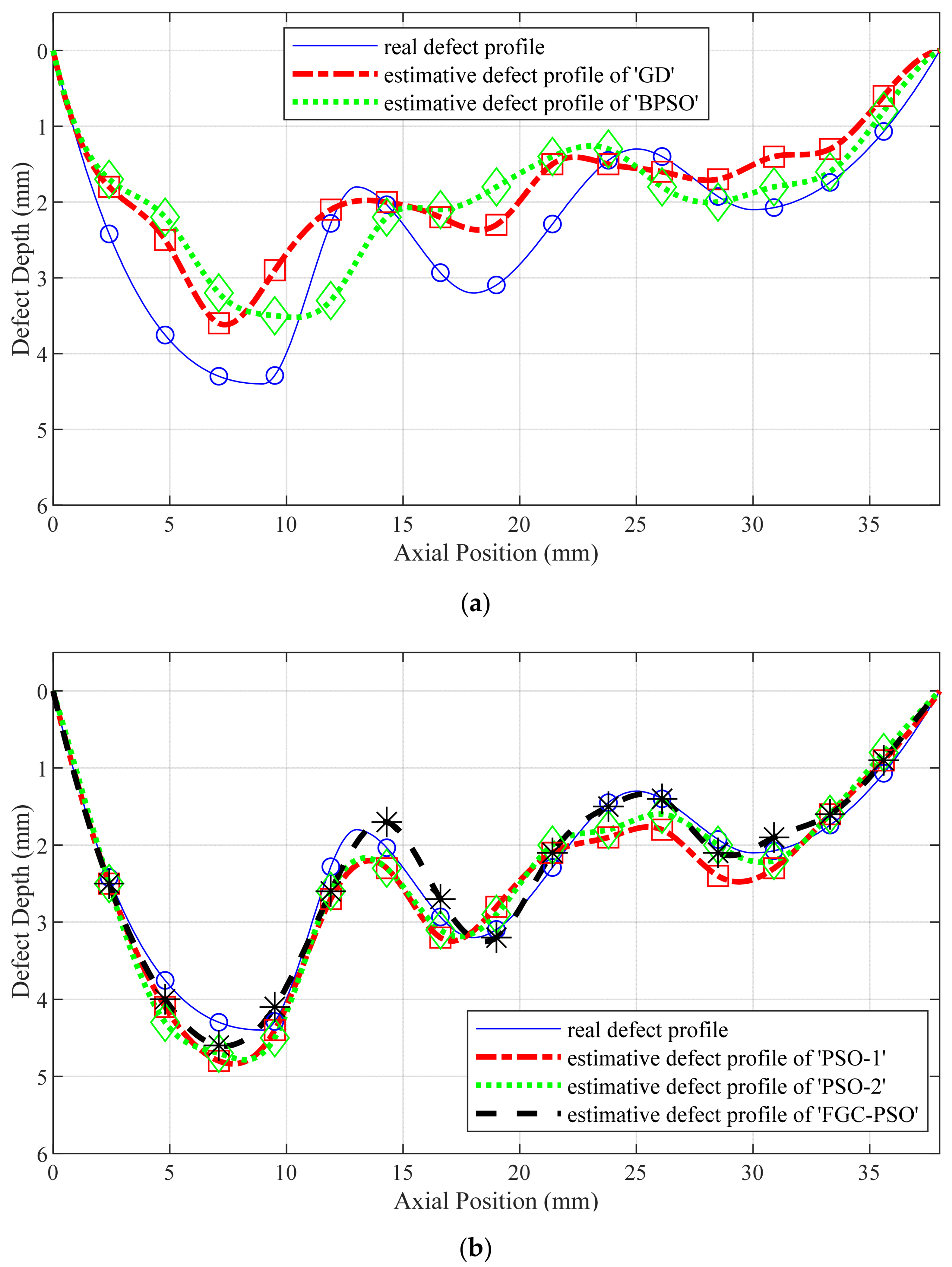
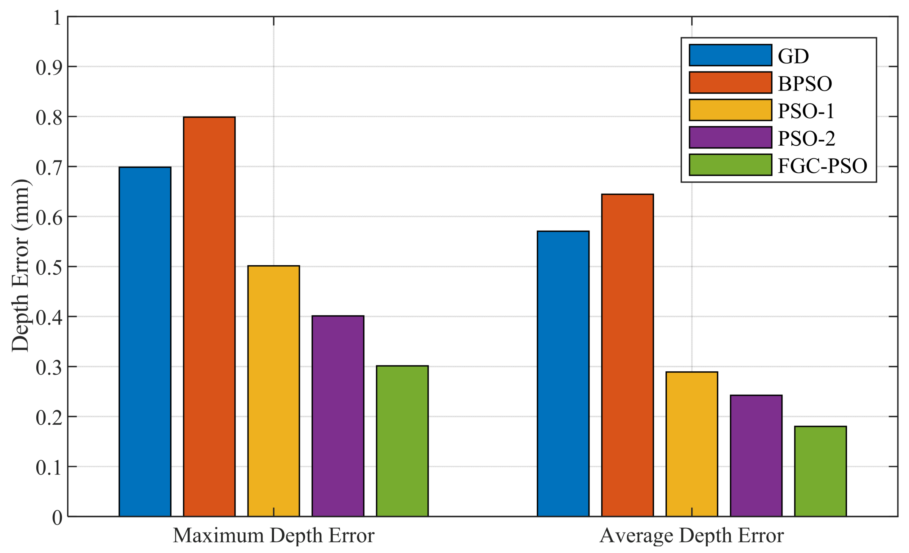
4. Experiment and Analysis

In order to verify the effectiveness of the method in this paper, a traction test, as shown in Figure 7, was carried out on a section of pipe with 40 defects. The outer diameter of the pipe was 219 mm, and the wall thickness was 8 mm. The structure and the material properties of the detector were the same as those of the above simulation, as shown in Table 1. Magnetic flux leakage signals of these 40 defects were collected by the MFL internal detector.

This paper designed two comparative experiments. The first compared the inversion accuracy of different methods under multiple degrees of freedom (multi-DOFs) for a non-standard defect to verify the global convergence accuracy of this method. Another experiment compared the convergence times of different methods in the inversion of 40 defects to verify the advantage of this method in terms of convergence speed.

4.1. Comparison Experiment of Inversion Accuracy under Multi-DOFs

A non-standard defect (as shown in Figure 8) was selected from the 40 defects as the target defect of the experiment in this section. The size characteristics of the defect were as follows: the length was 3.8 cm, the width was 1 cm, and the depth of the deepest point was 0.44 cm.

The iterative inversion of the defect is carried out under the three degrees of freedoms of 10, 13, and 15, respectively. The inversion results obtained by using the method proposed in this paper are shown in Figure 9. It can be seen from the figure that the method proposed in this paper can converge to the global optimal solution under three different degrees of freedom. Compared with the actual defect profile, the proposed method can reverse the accurate defect profile.

In addition, five different optimization methods were used to iteratively inverse the defect profile in Figure 10. The five methods are: 1. GD, the gradient descent algorithm; 2. BPSO, the basic particle swarm optimization algorithm; 3. PSO-1, the PSO algorithm with improved self-adaptive inertia weight; 4. PSO-2, the PSO algorithm with improved speed updating strategy; 5. FGC-PSO, the fast globally convergent particle swarm optimization algorithm proposed in this paper. The maximum number of iterations was set to 40 times with the defect DOFs of 15. The inversion results of these five methods are shown in Figure 10. The results of the statistical maximum depth error and average depth error are shown in Figure 11.

It can be seen from the figure that the error of the BPSO result is the largest. Due to there being too many optimization objectives, the optimization result of BPSO before improvement is quickly falling into local optimization. Therefore, even if the iteration time is increased, it is difficult for the BPSO algorithm to obtain an accurate inversion profile. The two-point improvement strategy proposed in this paper increases the search ability of global optimization based on the BPSO algorithm. The FGC-PSO algorithm can approach the optimal result, even in multi-objective optimization problems.

4.2. Convergence Contrast Experiment

In order to verify the convergence advantage of the algorithm proposed in this paper, for all 40 defects in the pipeline, iterative inversion was carried out under the conditions of 10, 13, and 15 DOFs, respectively. The optimization error of this comparative experiment was set to be less than or equal to 5 GS. If the number of iterations exceeds 100, it is considered to be unable to converge. The five methods used in this experiment are the same as those described above. The inversion results of 40 defects are listed in

Table 2. Convergence statistical results of 40 defects with 10 DOFs.

Algorithm Name	Number of Defects That Can Be Converged (Unit: Numbers)	Average Convergence Times (Unit: Times)
GD	35	48.4
BPSO	28	53.3
PSO-1	40	35.8
PSO-2	40	30.2
FGC-PSO	40	15.3

,

Table 3. Convergence statistical results of 40 defects with 13 DOFs.

Algorithm Name	Number of Defects That Can Be Converged (Unit: Numbers)	Average Convergence Times (Unit: Times)
GD	15	75.1
BPSO	8	87.0
PSO-1	35	49.8
PSO-2	33	38.1
FGC-PSO	40	23.9

and

Table 4. Convergence statistical results of 40 defects with 15 DOFs.

Algorithm Name	Number of Defects That Can Be Converged (Unit: Numbers)	Average Convergence Times (Unit: Times)
GD	0	-
BPSO	0	-
PSO-1	22	70.4
PSO-2	20	65.8
FGC-PSO	40	35.7

.

It can be seen from the table that when the degree of freedom is 15, the traditional methods cannot achieve the convergence goal of an error less than or equal to 5 GS. From the results of 10 and 13 degree of freedoms, it can be seen that the method proposed in this paper can achieve the globally optimal convergence goal with less convergence times. By comparing the experimental results of PSO-1, PSO-2, FGC-PSO, it can be seen that the three improved methods for BPSO show a certain improvement in the target convergence speed and accuracy.

5. Conclusions

This paper mainly solves the problem of pipeline defect inversion in MFL internal testing. Firstly, the finite-element model is used as the forward model, and then an improved particle swarm optimization algorithm (FGC-PSO) is introduced as the backward iterative convergence algorithm to realize the inversion of the arbitrary profile of defects. The FGC-PSO algorithm optimizes the traditional particle swarm optimization algorithm from two aspects: “self-adaptive inertia weight” and “speed updating strategy”. Among them, the self-adaptive inertia weight can fully tap the potential of each particle according to the inertia weight of the particle state. The improvement in the speed-updating strategy can increase the richness of the population and prevent it from falling into the local minimum too early. These two improvements can accelerate the convergence speed and raise the accuracy of the algorithm.

Due to the limitations of the forward model, this method can only obtain accurate contour inversion results when the defect width changes slightly (the width changes < 30% in the axial direction).

The axial magnetic flux leakage signal is used to realize the inversion of the defect profile in this paper. If the radial and circumferential signals can be combined, the inversion accuracy can be further improved, which is also the future research direction.

References

1. Lang, X.; Han, F. MFL Image Recognition Method of Pipeline Corrosion Defects Based on Multilayer Feature Fusion Multiscale GhostNet. IEEE Trans. Instrum. Meas. 2022, 71, 5020108. [Google Scholar] [CrossRef]
2. Feng, J.; Zhang, X.; Lu, S.; Yang, F. A Single-Stage Enhancement-Identification Framework for Pipeline MFL Inspection. IEEE Trans. Instrum. Meas. 2022, 71, 3513813. [Google Scholar] [CrossRef]
3. Jiang, L.; Zhang, H.; Liu, J.; Shen, X.; Xu, H. A Multisensor Cycle-Supervised Convolutional Neural Network for Anomaly Detection on Magnetic Flux Leakage Signals. IEEE Trans. Ind. Inform. 2022, 18, 7619–7627. [Google Scholar] [CrossRef]
4. Kandroodi, M.R.; Araabi, B.N.; Bassiri, M.M.; Ahmadabadi, M.N. Estimation of Depth and Length of Defects from Magnetic Flux Leakage Measurements: Verification with Simulations, Experiments, and Pigging data. IEEE Trans. Magn. 2017, 53, 6200310. [Google Scholar] [CrossRef]
5. Han, W.; Shen, X.; Xu, J.; Wang, P.; Tian, G.; Wu, Z. Fast estimation of defect profiles from the magnetic flux leakage signal based on a multi-power affine projection algorithm. Sensors 2014, 14, 16454–16466. [Google Scholar] [CrossRef] [PubMed] [Green Version]
6. Xu, C.; Wang, C.; Ji, F.; Yuan, X. Finite-element neural network-based solving 3-D differential equations in MFL. IEEE Trans. Magn. 2012, 48, 4747–4756. [Google Scholar] [CrossRef]
7. Li, M.; Lowther, D.A. The application of topological gradients to defect identification in magnetic flux leakage-type NDT. IEEE Trans. Magn. 2010, 46, 3221–3224. [Google Scholar] [CrossRef]
8. Lu, S.; Feng, J.; Zhang, H.; Liu, J.; Wu, Z. An Estimation Method of Defect Size from MFL Image Using Visual Transformation Convolutional Neural Network. IEEE Trans. Ind. Inform. 2019, 15, 213–224. [Google Scholar] [CrossRef]
9. Saha, S.; Mukhopadhyay, S.; Mahapatra, U.; Bhattacharya, S.; Srivastava, G.P. Empirical structure for characterizing metal loss defects from radial magnetic flux leakage signal. NDT E Int. 2010, 43, 507–512. [Google Scholar] [CrossRef]
10. Zhang, H.; Wang, L.; Wang, J.; Zuo, F.; Wang, J.; Liu, J. A Pipeline Defect Inversion Method with Erratic MFL Signals Based on Cascading Abstract Features. IEEE Trans. Instrum. Meas. 2022, 71, 3506711. [Google Scholar] [CrossRef]
11. Li, F.; Feng, J.; Liu, J.; Lu, S. Defect profile reconstruction from MFL signals based on a specially-designed genetic taboo search algorithm. Insight-Non-Destr. Test. Cond. Monit. 2016, 58, 380–387. [Google Scholar] [CrossRef]
12. Ramuhalli, P.; Udpa, L.; Udpa, S.S. Electromagnetic NDE signal inversion by function-approximation neural networks. IEEE Trans. Magn. 2002, 38, 3633–3642. [Google Scholar] [CrossRef]
13. Hari, K.C.; Nabi, M.; Kulkarni, S.V. Improved FEM model for defect-shape construction from MFL signal by using genetic algorithm. IET Sci. Meas. Technol. 2007, 1, 196–200. [Google Scholar] [CrossRef]
14. Lu, S.; Feng, J.; Li, F.; Liu, J. Precise Inversion for the Reconstruction of Arbitrary Defect Profiles Considering Velocity Effect in Magnetic Flux Leakage Testing. IEEE Trans. Magn. 2017, 53, 6201012. [Google Scholar] [CrossRef]
15. Li, Y.; Udpa, L.; Udpa, S.S. Three-dimensional defect reconstruction from eddy-current NDE signals using a genetic local search algorithm. IEEE Trans. Magn. 2004, 40, 410–417. [Google Scholar] [CrossRef]
16. Bergh, F.V.D.; Engelbrecht, A.P. A cooperative approach to particle swarm optimization. IEEE Trans. Evol. Comput. 2004, 8, 225–239. [Google Scholar]
17. Hsieh, S.T.; Sun, T.Y.; Liu, C.C.; Tsai, S.J. Efficient population utilization strategy for particle swarm optimizer. IEEE Trans. Cybern. 2009, 39, 444–456. [Google Scholar] [CrossRef] [PubMed]
Figure 1. Iterative inversion process of magnetic flux leakage for pipeline defects.
Machines 10 01091 g001
Figure 2. Finite-element model in magnetic flux leakage testing of defects.
Machines 10 01091 g002
Figure 3. Nonlinear B–H -characteristics of cold rolled X45 steel.
Machines 10 01091 g003
Figure 4. Axial and radial magnetic flux leakage signal of FEM simulation.
Machines 10 01091 g004
Figure 5. Flow chart of self-adaptive inertia weight algorithm in iterative inversion process.
Machines 10 01091 g005
Figure 6. Flow chart of improved speed updating strategy in iterative inversion process.
Machines 10 01091 g006
Figure 7. Photos of the test field and MFL internal detector. (a) The traction test field; (b) The MFL internal detector.
Machines 10 01091 g007
Figure 8. The picture of the non-standard defect.
Machines 10 01091 g008
Figure 9. The real defect profile and the calculated inversion profile with different DOFs. (a) DOFs of 10; (b) DOFs of 13; (c) DOFs of 15.
Machines 10 01091 g009
Figure 10. Defect profile curve estimated by five optimization methods. (a) ‘GD’ algorithm and ‘BPSO’ algorithm; (b) ‘PSO-1′ algorithm, ‘PSO-2′ algorithm and ‘FGC-PSO’ algorithm.
Machines 10 01091 g010
Figure 11. The statistical results of maximum depth error and average depth error.
Machines 10 01091 g011