Intelligent Mechatronics in the Measurement, Identification, and Control of Water Level Systems: A Review and Experiment

Abstract

In this paper, a unique overview of intelligent machines and mathematical methods designed and developed to measure and to control the water level in industrial or laboratory setups of coupled and cascaded configurations of tanks is made. A systematized and concise overview is made of the mechatronic systems used in the measurement, identification, and control of the water level enumerates, the software used in the associated scientific research, modern techniques and sensors, and mathematical models, as well as analysis and control strategies. The broad overview of applications of the last decade is finalized by a proposition of a control system that is based on a parameter estimation of a new experimental setup, an integral dynamic model of the system, a modern mechatronic machine such as the Watson-Marlow peristaltic pump, the Anderson Negele sensor of level, the NI cRIO-9074 controller, and LabVIEW virtual instrumentation. The results of real experimental tests, exploiting a hybrid proportional control, being improved by a numerically predicted water level, are obtained using a few tools, i.e., the static characteristics, the classical step response, and a new pyramid-shaped step function of a discontinuous path-following reference input, being introduced to evaluate the effectiveness and robustness of the regulation of the level height.

1. Introduction

Liquid level control is a dynamic problem that occurs in various branches of the mining, food, processing, and transport industries, as well as at the level of the vast living environment of humans and animals, e.g., in tanks built by humans. Thus, the effectiveness of automatic control systems affects not only the functioning of devices and processes managed by man, but also the quality of life in an environment controlled by humans. The subject matter of this work is constantly developed due to new measurement tools and more efficient microcomputers, the performance and programming methods of which are evolving very quickly. Concepts include, for example, projects based on the wireless observation of dynamic phenomena, and the monitoring of production lines. In connection with the above—the constant development of methods of producing and storing liquids, it is necessary to transfer the already existing methods of controlling dynamic processes, and to improve and to embed them into new programming environments using modern programming techniques involving more advanced control algorithms, based on numerical models imitating the real state of the tested object.

Thus, the objective of the work is to make an extensive, but a concise and unique overview of the intelligent machines and mathematical methods that have been designed and developed to measure and control the water level in various configurations of tanks. The up-to-date overview will be split into a few sections devoted to the main parts of most designs, including computer software, mechatronics hardware, mathematical modeling and some strategies of control of liquid level in a single-, two-, or even multi-tank systems. Next, we present a real laboratory test setup in which modern mechatronic hardware is implemented and equipped with an automatic hybrid control system. The obtained system allows for the introduction of a numerical model and the prediction of the actual water level, increasing the accuracy of the regulation process. We subject the proposed system to two tests, where one of them engages a new pyramid-shaped step function—a discontinuous path reference input.

We organize the remaining part of the manuscript as follows: Section 2 describes the software used in the scientific research of liquid level control systems. Then, Section 3 covers modern techniques, hardware implementations, and sensors for water level measurements. Later on, the mathematical modeling of a single-, two- and multi-tank dynamical systems are formalized in Section 4, which are gained via a state-of-the-art analysis of the model and control strategies described in Section 5. At the end, Section 6 presents the results of our experimental attempts upon the proposed system of control that has been embedded in a configuration of the National Instruments (NI) hardware platform.

2. Software in the Research of Liquid Level Control Systems

There are many possibilities of numerical coding in the realization of virtual or real systems of liquid level control. One can simulate such models in any programming language, or even in MS Excel. The hardware side that is represented by microcontrollers (microprocessor units [1]) creates the logic unit that is able to compute the controlling output accordingly to the prescribed algorithm, operating on inputs coming from the SISO or MIMO object of control. Programs on microcontrollers are installed in on-chip memory. We use processing compiling machines to transfer the codes of a high-level languages into a code that is understood by the machine. Then, it is stored in the appropriate electronic units managed with the memory. We can process it in a few ways. It can be pre-programmed, obtaining a status of a read-only memory, it can be treated as a flash memory, being a field-alterable one, or even like the reconfigurable field-programmable gate array of embedded systems, of which a very modern approach represented by the LabVIEW environment is considered later in our work. It is mostly coded with the use of C, FORTRAN, or Pascal languages, which stand for some examples of high-level languages (HLL), and also very HLL (VHLL) languages such as Perl, Ruby, Visual Basic, and Python. Usually, engineers try to look for an easier representation of control schemes. Therefore, mostly MATLAB/Simulink and LabVIEW, or rarely, Scilab/Xcos environments with a visual interface in a block diagram form, as well as JavaScript and C++, support their investigations. Before we present and describe our block diagram, let the following applications be enumerated.

2.1. MATLAB/Simulink Environment

A mathematical model of a liquid level in a tank of varying size is derived in [2]. According to some proportional-integral-derivative (PID) parameters, the model was simulated with the use of Simulink software.

Since any tank system is inherently nonlinear in a wide range of process variables, the PID controllers are generally noticed not to be efficient in tracking control on a wider range of water level. Therefore, many papers analyze the effectiveness of the regulation of the liquid level height using the fuzzy logic (FL) approach. In one of them, see [3], the controller of a fuzzy type is applied in a mathematical model implemented in Simulink—a fronted tool for the visualization of block diagrams under the umbrella of MATLAB software. The most interesting aspect is that the controller has been programmed in an embedded system equipped with an ARM microprocessor on Arduino. The development board serves as the system of sensor data acquisition from the Festo didactic tank system. A generator of PWM—pulse width modulated signal, controls the volumetric outflow of the water pump.

From modeling and simulating the level control in a water tank, the FL approach has been considered [4] by Omijeh et al. In order to successfully achieve the design and simulation of a FL-based controller that will provide a stabilized output response, the Fuzzy Logic Toolbox package of MATLAB and the Simulink environment are implemented.

In paper [5], the identification of a water level system using an FL inference system with the adaptation of the network for the modeling and control of this object is proposed by Turki et al. The model and its control have been performed in MATLAB/Simulink, where the numerical and real models have been compared. In the study continued in [6], the authors tuned the Takagi-Sugeno (T-S) neuro-fuzzy liquid level control system using PSO—Particle Swarm Optimization.

The proportional and PI regulation of the water level in a tank was presented in [7]. The authors performed a modification of exact linearization, which was based both on an unknown model dynamics, as well as on an integral action, stating a nonlinear observer of disturbance. As in previously mentioned cases, the system was visualized as a block diagram and simulated in Simulink.

The teaching of advanced control topics using a nonlinear MIMO—multiple-input and multiple-output system of a three-tank model was studied in [8] by Rosinova et al.

The work by [9] is worth attention. The authors analyze the problem of control design with an observer of the state of a four-tank water level CTS. A simulink supported with some real-time libraries available in a host environment was successively used to build a real-time control loop, dealing with the control and observation of the states of the CTS. One may note the crucial serviceableness of MATLAB/Simulink, and also other packages such as LabVIEW and Scilab/Xcos, that is, the experimental validation. Being applied in simulations after the implementation of control laws, the structured graphical interface is user friendly, and in most cases, much more intuitive for engineers than any written code. A C++ program from the Simulink model is built using a real-time workshop using Keil $\mu$Vision to produce a program for the direct execution on the CPU. A real-time Windows target module connects to the program with the designed controller implemented, and also physically interfaces with the CTS via a microcontroller board.

The work [10] deals with an efficient controller, utilizing a quadratic programming approach in a multi-dimensional parameter space applied to a quadruple-tank system (a process). The nonlinear 4-CTS is modeled using a transfer function of the Laplace variable, while the performance of its control system is evaluated based on the Simulink process model as well.

Analytic and experimental investigations under the FOPI—fractional-order PI controller designed in the frequency domain, are presented in [11]. The controller is referenced to a few traditional controllers, either PI or PID, with two or three degrees of freedom, proving its superiority over the controllers with the same type of control loop. The level sensor’s outputs are made available on a PC inside Simulink through an interfacing card. The frequency domain approach used in the design to elaborate the closed-loop transfer function for the FOPI and its concurrent controllers is achievable in MATLAB with the use of an environment-integrated SISO tool.

The control algorithms of many variables forcing the maintenance of the desired levels of the closed- and open-loop 2-CTS are taken into consideration in [12]. A Simulink simulation equipped with the dedicated MATLAB functions served as the programming environment of the system.

In the context of automotive (not stationary) fuel tanks, a few architectures of NN—Neural Networks are investigated using MATLAB in [13] by Terzic et al. The networks were trained using the training function trainlm, the frequency coefficients of which were obtained in a preliminary processing with the data using the FFT function.

MATLAB can be used to validate the efficiency of the intelligent FL controller of the second type, as was shown in [14], on the basis of level control in a hybrid 3-tank system.

The model prediction approach marks an important direction in the control and identification of many dynamical systems, such as that mentioned in this work. The control of nonlinear MIMO dynamical systems oriented on the regulation of water level with the use of the PID or RK-PID—Runge–Kutta PID controller in a discretized form is proposed in [15]. Real-time control platforms operated from Matlab and Simulink have been applied to build highly effective and fast numerical procedures of the regulation of water level.

In [16], a NN-based controller is verified on the background of a water-tank Simulink model using mathematical modeling and control of the object of control in RT—real time. A good degree of accuracy of tracking for the reference water level for all set-points was noticed, being maintained by the designed control system.

A typical existence of a weakly nonlinear behavior is reported in [17] in a laboratory setup created by water tanks arranged in a cascade configuration. Soft and hard nonlinearities that were combined in the configuration were identified based on relatively short-term records of measurement data. MATLAB was used in the setup to identify the controller of the water levels based on the sensor and the pump being interfaced by analog-to-digital and digital-to-analog converters (ADC and DAC).

The dynamic patterns observed in the response of control genetic circuits are often modeled using the Hill function. One notes that authors of the work [18] applied an integral Hill controller to regulate the level of a conical tank. Good performance was proven after a comparison of the controller with the PI and PID controllers of various kinds tuned in MATLAB CT with the use of the Ziegler–Nichols experimental method. Another attempt for a basic design of a PID controller tuned online in using by the GA—genetic algorithm applied to the water level single-tank-reservoir system is shown in [19].

A T-S type FL controller with a PLC—logically programmable controller is used in [20] to regulate the levels in the tanks. The optimization of the parameters of the very popular FL controller was performed using the Cuckoo optimization algorithm, where MATLAB served to tune the optimal parameters of the membership functions, since a simulation of control of the liquid level was carried out in Simulink. Worth noticing is the PLC-based water level control performed in [21]. Although the presented results do not fully exhibit the effectiveness of the proposed application, an interesting hardware of a closed loop has been used.

MATLAB toolboxes are very useful. As a subsequent example, the toolbox for solving LMIs—linear matrix inequalities, can be employed in order to deal with many problems of semidefinite programming. The authors of [22] implemented it to satisfy the robustness of a model-predictive control, called the MPC method. The most important challenge usually lies in the uncertainty of the model. Realizing this feature, an additional time delay was injected into the control procedure coded in MATLAB.

The article [23] presents an analysis of three classical PID algorithms, i.e., the linear, fuzzy, and NN controllers. The efficiency of the tested control procedures was assessed using the dedicated laboratory setup, involving a cascade of two tanks and a reservoir. Implementations of control algorithms have found their realization in MATLAB/Simulink, communicating with the Advantech card PCI-1710.

Let us now conclude Section 2.2. The presence of MATLAB/Simulink in research oriented on the intelligent interfacing of hardware with the described experimental setups of many realizations of CTS is still very strong. Moreover, its scope of computational applicability, together with interactions with measurement hardware that fit to the software’s libraries and toolboxes, as well as to the embedded systems of many producers, significantly increases. Scientists and control engineers like its simplicity, the rapid prototyping of block diagrams, and its reliability, because they do not need to deeply specialize in programming languages and the usage of libraries necessary to connect any measurement cards or microcomputers to their test setups. The applications and exploitation of the environment with its developing tools, supporting many engineers, will grow in time, being still a competitive one for the quickly developing and industrially oriented LabVIEW environment described in the following subsection.

2.2. LabVIEW Virtual Instruments

One of the fast-growing programming platforms is LabVIEW—a system that integrates the creation of front panels and virtual instruments, saved as separate files belonging to larger computing projects. The advantage of this environment is ensured by, among others, multi-node processes and a graphical representation of the numerical code compiled into an executable program communicating with measuring devices. The software includes many possibilities for defining problems and their representation using block diagram, Stacked Sequence Structure, MathScript nodes, MATLAB or Python, and many others. The HMI user interface is event-driven, and allows for a visualization of the variables associated with different displays of values [24].

The software in question appears to be complete, as it provides: (i) the visualization of components; (ii) the testing of various control strategies; (iii) the obtaining of data; and (iv) communication with various electronic devices.

The implementation of a digital PI controller for a CTS focused on water level control is carried out in [25] by Bastida et al. The model parameters were identified using sinusoidal signals of different frequencies. This made it possible to draw a Bode plot to design a digital controller in LabVIEW. The controller can send small gains, allowing for the flexible adjustment of overshoot and the rising time.

The implementation of FL and PID controllers developed in the LabVIEW environment to solve the problem of water level control was completed in [26]. The traditional PID algorithm was implemented and tested to correct the steady error, and then FL controllers with higher efficiency and stability were studied. The following results were obtained: the elimination of overshoot, better tracking of the set-point, and as a result, a shorter time of determining the system response, with smaller errors computed on the basis of the integral criterion.

Another FL controller, together with its input/output membership functions has been implemented in LabVIEW in [27], using the very useful Control and Simulation Toolbox. It is the basic tool of control engineers practicing with numerical simulations performed in the environment. A closed-loop block diagram considers the nonlinear spherical tank level control process, level transmitter, I/V and V/I converter, NI USB DAQ 6001, a pneumatic control valve, and a rotameter. The designed FL controller covers the entire range of the spherical tank level height, while a deviation of process variable to the set-point in the steady state is estimated to be less than $\pm 2\%$.

Remote access for an experimental water level control in a 2-CTS with the support of the LabVIEW Smartphone Communication Toolkit is realized in [28]. The output of a PID regulator has been fuzzified using a particular logic written in a MathScript node for some configurations of solenoid valves that have maintained the two reference levels of water.

A water clarity and volume monitoring system of a tank was a subject of an experimental work [29]. Dealing with the detection of water level, the authors implemented a sensor of ultrasonic waves (RF04), since dealing with detection of water clarity, they employed a sensor of turbidity, which was controlled by NI myRIO-1900. An automatic relay module (a terminal), being a part of the NI controller, was introduced in the water-tank system and integrated with a LabVIEW running on a PC acting as an HMI. As is often observed, also in this work, a remote monitoring system has been realized in a local Wi-Fi network.

The work conducted in [30] is devoted to an application of the control software for a multipurpose tank system, and also to the development of the inspection techniques to teach the fundamentals of monitoring systems and control engineering. In this case of an experimental study, the flexibility and high level specifications of LabVIEW decided to select it as the monitoring interface, since the main control tasks have been assigned to industrial controllers. The LabVIEW interface operating as an acquisition system, namely the supervisory control and the data acquisition (SCADA system), allowed one to remotely regulate the level height and monitor the process from the PC.

Usage of LabVIEW for data acquisition (DAQ), user interfacing, and process monitoring was required in [31] during the experimental works under a level sensor based on the bending of an optic fiber Bragg grating—the so-called FBG. One observes a similar application of the software in [32] to obtain and process with experimental measurements of water level, for instance, while building a cross-correlation algorithm, where another water level optical sensor, being designated for large range measurements and connected to an instrument integrating optical sensing, has been developed.

Digital displays that inform drivers of automotive vehicles about fuel consumption and the distance that they can travel before a next fueling incorporate practical fluid level measurement systems. One of them, permitting an accurate determination of the fluid level in a dynamic environment, is described in [33]. Older solutions of such measurements preferred mechanical mechanisms, since in the very new ones, an ultrasonic sensor of water level is adopted. In the mentioned experiment, it generates a voltage signal that is acquired by a card of signal acquisition communicating with the LabVIEW software.

The data flow model offered by the LabVIEW graphical programming idea is used in [34] to program the Arduino UNO microcontroller (a development board). It stands for an interface between the components of the electronic circuits and the software. The board operating based on the LabVIEW program detects the level using ultrasonic sensors, as well as controlling the relay circuit at any predefined water level limit values.

We may note that usage of front panels is a common practice of many applications of the software, since its use for signal conditioning is still not fully explored and developed. Therefore, a fact worth noticing is that in the simulation diagram, the authors applied a LabVIEW flat sequence structure to command the relay circuit, turning the water pump off, as well as building a special virtual instrument to acquire data from the ultrasonic sensor.

Finally, let us mention some investigations completed in [35], where a new NMPC—nonlinear model-predictive controller, working in RT, to regulate a multi-degrees-of-freedom CTS, is elaborated. The researchers applied a DAQ device NI-6009 coupled with LabVIEW to acquire streams of data (a multi-input control of levels in both tanks) from sensors in RT.

This subsection brings some interesting conclusions. The LabVIEW environment proved its high usefulness as the well-integrated development tool, supporting the observation, measurement, signal conditioning, numerical simulation, detection, and control of water level in CTS. Its field of application expands very quickly due to the completeness, reliability, and also ability to various reconfigurations of the user interface, real-time operations, integrated packages of measurement devices, continuous development, and growing popularity within the engineers. Having this in mind, the authors of this paper decided to interface their experimental test setup with the LabVIEW environment and NI hardware. This intelligent realization of the mechatronic system is briefly described in Section 6.

2.3. Other Programming Environments and Languages

The main objective of the study carried out in [36] by Alvaro et al. is to regulate the level of water in a system of tanks using Xcos software. As usual, the mathematical modeling of the dynamic response of each tank is based on the mass conservation equations. At a later stage, the identification of the control variables and disturbing factors was carried out.

The work [37] deals with a wireless MPC of a water level control system (see also [29] for a wireless application). With respect to the mostly existing saturation limits, the objectives of the control target the maintenance of water level around the reference set-point values. A wireless mode control algorithm oriented on that aspect is implemented using C++ language.

Program design in the IDE—integrated development environment using C language on an Arduino Mega 50 pin I/O microcontroller has been carried out in [38]. The presented research aimed to design a trainer simulator of the water level measurement using the microcontroller integrated with HMI. See also [29] for another exemplary exploitation of the HMI working as a monitoring tool.

The paper [39] presents an innovative approach for carrying out automated experiments, expressing an idea of a VL—a virtual laboratory. VLs for some educational purposes, studying the water-tank system, are developed and executed using the experiment editor elaborated in Java-based VLs created with the use of Easy Java/JavaScript simulations. The presented IDE is open for data gathering from the tasks subjected to an automation and statistical analysis.

To sum up Section 2, MATLAB/Simulink and LabVIEW are the most commonly exploited environments in the modeling of dynamical systems conjugated with the design of virtually realized control systems, which are connected with real tests or industrial setups subjected to many kinds of theoretical analyses and control strategies. Next to the mentioned rapid prototyping packages, there exist in the branch of applied mechanics and mechatronics, the Scilab/Xcos environment, which is slowly growing in popularity, and also some general purpose programming languages such as C++ or Java, allowing for the creation of highly customizable programs. Many simulations or programming environments are not described by the authors of scientific works, since they do not decide to mention the tools that they use in their investigations. Nevertheless, the overview reveals many possibilities and areas of application of the inspected software.

3. Modern Techniques, Machines, and Sensor Solutions for Water Level Measurements

Real applications reveal many methods for measuring and regulating the liquid level. The measurement techniques must meet the requirements of modern technological processes. The real-time measurement of the water level is possible, e.g., with gauge pressure transducers. The use of mechanical measuring devices such as differential pressure sensors and level gauges based on a hydrostatic measuring method, and capacitive sensors or optical grating are often selected [5,40,41,42,43]. On the other hand, non-contact measurement techniques without electrical connections inside tanks are being developed [32,33]. However, this approach is not effective in controlling chemical reactions in liquid tanks. For example, to remedy this, measurement techniques based on image acquisition conducted in [44] (see also a review [45] with references) have emerged that have proven their high resolution stability at low cost. In the following chapters, we highlight new developments in the field of capacitive, visual, fiber-optic, and ultrasonic tank fill level detection.

3.1. Capacitive-Type Sensing

There are not many state-of-the-art reviews and evaluations of the performances of low cost measurements in the tank systems. One of them is reported in [46], where a short inspection of the techniques for the sensing of liquid level is performed. The study shows that the idea of measurements at very decreased costs of the software and hardware (overall equipment) is relatively poorly explored. In a drawn conclusion, special high-cost equipment is required for the conditioning of electric signals and processing with the acquired data generated by various sensors of level. On the background of a few solutions of sensor designs (for instance, see the capacitive-type sensing mentioned in [47,48,49]), the authors boldly proposed a sensor made of three-layer polyethylene tubes. The sensor, consisting of two insulating materials and a metal material between them, is made concentrically with slightly differing diameters of cross-sections of the tubes. Vertical placement of the two tubes permits stable measurement, as well as protecting the sensor from the troublesome noise of parasitic capacitance. A particular description that is devoted to the high accuracy measurement of capacitance of the sensor and an interesting circuit for signal conditioning with operational amplifiers is presented. After a careful demonstration of the performance, the elaborated capacitive water level monitoring has revealed a quality that is comparable to the very popular ultrasonic techniques of sensing.

A non-contacting device of a capacitive principle of operation, which is proposed for water level detection, is fabricated from two copper plates, as described in [50]. The sensor is characterized by a high impedance (at low frequency) that results from the impedance expression for the capacitor. The solution can find an application for the quantification of water level from electric characteristics, which is in inverse proportion to the impedance of the sensor (the dielectric constant between the two plates is proportional to the height of level). The conditioning of the signal is made on the way of linearization, inverted amplification, and the usage of rectifying circuits. As a result, a relationship between the capacitance, the water level, and the output voltage is delivered.

A water level measurement of a different kind using an digital capacitive sensor, integrating two interpenetrating comb electrodes at low costs, and the consumption of energy, good linearity, and repeatability can be found in [51]. The spacing between each comb electrode causes variations in the capacitance at changes of water level. The capacitance of the comb electrodes in terms of the time of discharge related to the measured level is estimated using a microcontroller. The presented technique does not need re-calibration, since the sensor can deal with the absolute measurement of water levels at a resolution of 0.2 cm, and in the 30 cm range. The paper contains a deeper literature overview devoted to other capacitive sensors for liquids, as well as to contrary techniques, such as TDR monitoring, FBG embedded in cantilever, fiber optic sensors of the liquid level, and Fabry-Pérot and FBG pressure sensors.

Let us conclude this part. Capacitive sensing devices are the relatively simple low-cost sensors characterized by small dimensions and the low consumption of power at non-complicated manufacturability. Despite the above, the use of capacitive transducers is limited. Being the proximity sensors, they are not effective in dusty and chemical industries, because their responses are subject to significant variations in the presence of pollution and aggressive media. Image-based, optical, or ultrasonic sensing, described in next section, can overcome many of these problems.

3.2. Image-Based and Optical Sensing

An opto-fluidic sensor for the measurement of liquid level has been demonstrated in [52]. For the first time, the authors presented an ECVFL—an electronically controlled variable focus lens that changes the profile of the spatial intensity of the optical beam falling on the liquid surface, and simultaneously conserving low power requirements. The surface of the liquid reflected an intensity profile for reaching its smallest size, while by tuning and measuring, the liquid level was estimated according to the size of a beam spot varying versus the calibration table of ECVFL focal length. In opposition to the mentioned ultrasonic sensors, this non-contact sensor, utilizing a non-modulated radio frequency, is useful for hazardous fluids. Focusing our attention on the reviewing perspective, many references have been provided to the non-contact level sensing techniques using computer vision, optical radars, or optical fibers.

Mainly with regard to new numerical achievements in image recognition and the appearance of low-cost industrial cameras, the measurement of fill levels in miscellaneous water tank systems, including the monitoring of their physical status using recorded images of the object of control, develops very quickly. One of such attempts, presenting an innovatory measuring system based on image recognition, is proposed in [53]. Above the tank with liquid, the authors installed a digital camera and found a relation of the pixel counts of liquid float in the image to the distance, at which the pictures were taken. It was shown that during the monitoring of the process in the tank, the author system could precisely measure the level using the recorded images. One can also read in the mentioned references about several competitive solutions. Other high precision automatic measurement based on processing with images can be found in [54], including fiber-optic liquid level sensors in [43,55,56].

Next to the above small-scale applications, many environmental solutions of civil engineering do exist in surveillance cameras [57], which make single-camera images, providing the field monitoring of the water level at rivers and hydraulic facilities.

3.3. Ultrasonic Sensing

These kinds of sensors are widely employed, being installed above the process tanks. They are simple and safe for use. Moreover, the guided ultrasound sensors can be operated robustly for a long time. None of the sensor elements come into contact with the liquid; therefore, it can be used in many applications, including aggressive media. Moisture, temperature, and pressure have some impact on the accuracy of measurements performed with the use of these sensors.

For instance, in [58], the sensor’s speaker emits high-frequency 40 kHz acoustic waves that reflect against the fluid’s surface and that return back to the transducer’s sound receiver (a microphone). The electronics measures the time of transition of the reflected signal to determine the height of the liquid level. An ultrasonic sound wave is emitted in 200 $\mathsf{\mu }$s of time and in the frequency of 40 kHz. Propagating at the speeds of 1/29.034 cm/$\mathsf{\mu }$s, the sound wave detects the level surface at some height, and then it reflects back to the ping sensor, which generates a pulse while waiting for the reflected wave. The sensor’s generation of pulses stops when the reflected sound is detected. This way, the distance between the sensor and liquid surface can be seen in terms of a changing width of the waiting-state pulses. Finally, the microcontroller is able to measure the width of the generated pulses and convert them into the distance. The applications of such intelligent sensors for the purpose of detection of water level can be extended on a wireless communication, in which the data are collected remotely.

An interesting solution exploiting the ultrasonic transducer and the wave guide rod is demonstrated in [59]. The level of the liquid is mainly proportional to the time of traveling of the wedge wave. The so-called interface echo method is described by a 0.39 mm of deviation at the 0.12 mm level of uncertainty, which is smaller than the industry standards. There was an electric noise observed, such as the variation of the water level (due to variations in the liquid surface) and the droplets of water, having not so much effect on the accuracy of the contactless measurement. In practice, sufficient accuracy and high resolution at a low cost and high safety have been reported by inventors of the sensing method.

Another measurement technique of an accurate sensing of water level, finding its application in dynamic environments, is mentioned in Section 2.2 [33], since many more, using the physical mechanism of the acoustic wave propagation is shown in the paper [59]. Other applications of an ultrasonic sensor, and cooperation with Arduino UNO and LabVIEW software, are performed in [34].

To sum up Section 3, we have performed a short inspection of the sensors and their associated hardware environment applied to the measurement of water level. Each of the techniques enumerated in Section 3.1–Section 3.3 have their own special destination, the features of which are used in some dedicated or more general realizations of fill level detection and and monitoring. We referred this part of our overview only to the newest achievements in sensing and processing with the physical signals, such as mechanical, electrical, optical, or even visual ones. Their common feature is distinguishable in the exploitation of modern materials and electrical engineering. For instance, miniaturization reflected on the microcontroller boards allows for the embedding of more or less sophisticated mathematical algorithms, e.g., performing geometrical or analytic computations on the data collected by the sensors in electric form. The very expanding use of the microcomputers makes the mechatronic measurement systems more intelligent, allowing much more complex mathematical transformations to be realized, including simple calculus, estimation, prediction, numerical integration, etc. Some of the most important ones are studied in the next section.

4. Mathematical Modeling

Typically, the mathematical modeling of a single tank is straightforward, although the models of any coupled or cascaded tank systems are nonlinear due to the series connection of the individual tanks. In both cases, nonlinearities are transferred via the dynamic response of valves, pumps, and sometimes sensors. The derivation of the models is based on the mass or volume flow balance (or mass or volume conservation) equation, estimation of flow resistance on contraction lines, the Bernoulli continuity equation, and valve inlets and outlets, while less often on tank geometry. It is also based on estimating the efficiency of the water source if the height of the water in a tank placed in a gravity field is higher than the height of the water tank. A single tank or a system of tanks can be understood as complex lines of inertial, most often gravitational, flow of media filling them. They are modeled as single integral automation elements or as multiple integral elements arranged in series when two or more cascaded tanks are considered.

This section begins from the enumeration of a tank system configurations designed and explored in state-of-the-art engineering research and educational applications. Then, some mathematical models embracing the most popular ones are delivered.

We have selected an up-to-date literature by splitting our study into three cases differing in complexity for the object of control:

1.

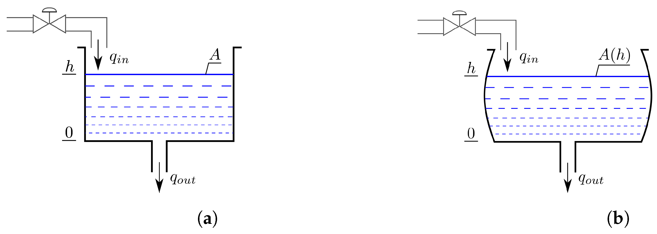
A single-tank dynamical system (eventually, equipped with a reservoir—a basin of water), which is investigated in [39,60,61] (state-space approach, PI, PID), [22,37] (state-space representation in a discrete form), [2,7,19,26,62,63] (transfer function approach), [3,5,6,26,62,63,64,65] (FL, PSO), [22,37] (predictive control), [18,20,27] (geometry-varying tank: conical and spherical) and others [34,46];

2.

A coupled or cascaded two-tank dynamical system, which is investigated in [17,66,67,68,69] (state-space approach, PI, PID), [11,12,23,25,30,36] (transfer function approach), [35,70,71] (FL, PSO, NN), [72] (autoregressive model), [73] (multidimensional regularization), [74] (model-predictive control of a geometry-varying conical tank), and [75,76] (SMC);

3.

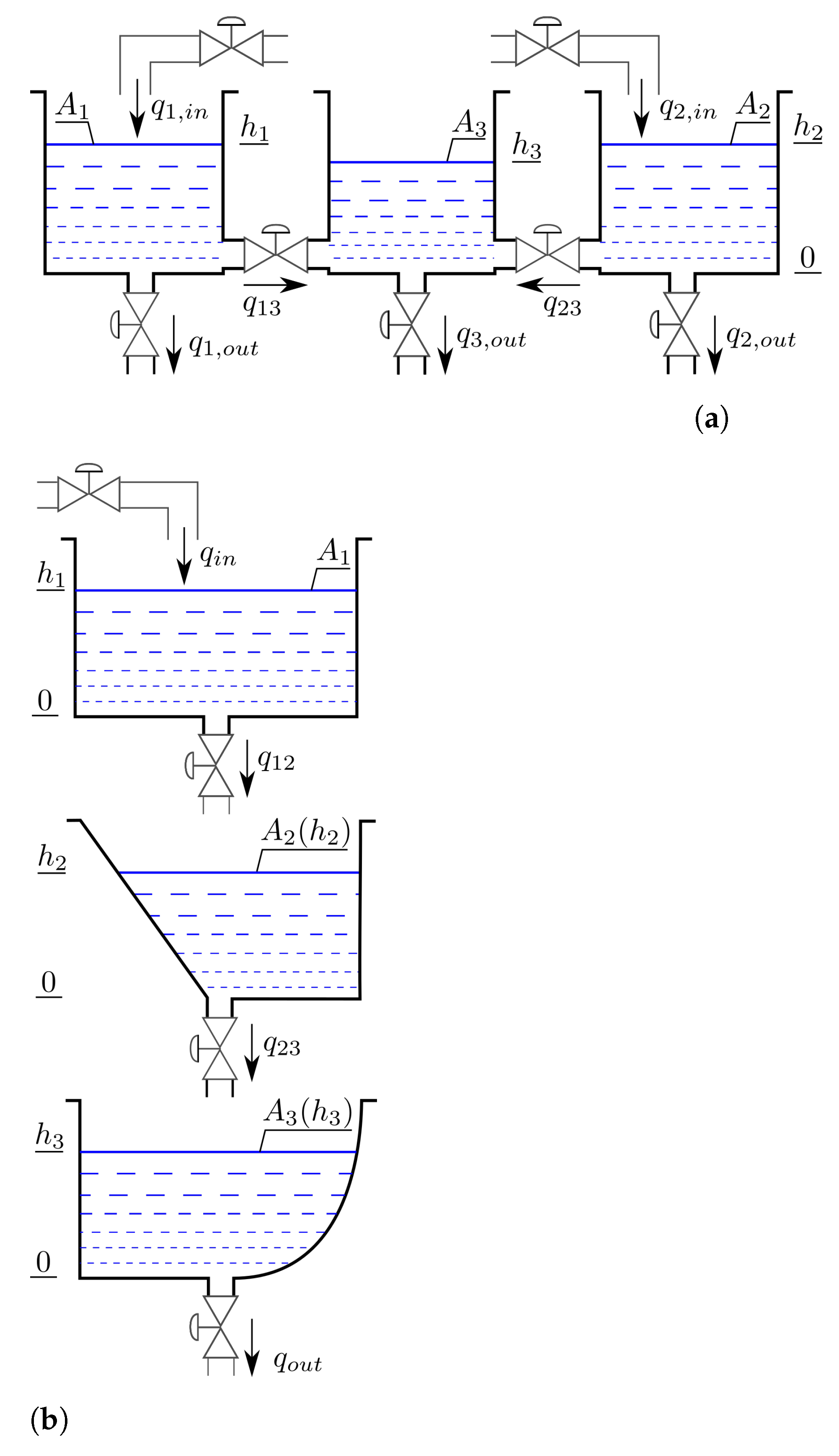
A coupled or cascaded dynamical system consisting of many tanks, which is investigated in [8,15,68,77,78,79,80,81,82] (state-space approach, PI, PID), [10,30,80] (transfer function approach), [14,16] (FL, NN), [9,10,15,78,83] (model-based or model-predictive control, state predictor), [8,16,79] (geometry-varying tank), [77,84] (SMC), and [80] (dead-time).

4.1. The Single-Tank Dynamical System

A schematic representation of a known model of the physical water level control process based on a single outlet and controlled inlet of a tank is shown in Figure 1a,b (taking into account the varying cross-section).

Let the inflow to the tank change, as shown in the Figure 1a. Assuming that, in the steady state of the linear dynamic process, the inflow to the tank is regulated by a proportional regulator, and the flow will depend on the inflow pressure [60]. The mathematical notation can be given in a linear form by connecting the flow regulator in series with the water level regulator.

The assumed balance of the water mass in the tank allows us to write the first-order differential equation

$$A\rho \frac{dh\left(t\right)}{dt}={\tilde{q}}_{in}\left(t\right)-{\tilde{q}}_{out}\left(t\right),$$

(1)

where the level height is denoted by h, ${\tilde{q}}_{in}$ is the rate of mass flow to the tank (a mass inflow rate), ${\tilde{q}}_{out}$ is the rate of gravitational or forced mass flow of discharge (mass outflow rate), A—constant cross-section area of tank, $\rho$—density of liquid, and the time derivative $d(·)/dt\equiv \dot{(·)}$ is the rate of level changes in time. At an assumption of incompressibility of the liquid, the model given by Equation (1) can be rewritten in terms of volume conservation in the tank, using the system of state-space equations:

$$\begin{array}{cc}\hfill \dot{h}\left(t\right)& =\frac{1}{A\rho }\left(q_{in}\left(t\right)-q_{out}\left(t\right)\right)\mathrm{with}h\left(0\right)=h_0,\hfill \\ \hfill y\left(t\right)& =h\left(t\right).\hfill \end{array}$$

(2)

The rate of volume flow that discharges the tank (volumetric outflow rate) is denoted by $q_{out}$, since $q_{in}$ is the rate of volume flow charging the tank (volumetric inflow rate).

The model introduced in Equation (2) is often practiced in the control of water level only. While operating with chemical reactors, the model in Equation (1) is most frequently used. Both equations in the system (2), i.e., the ordinary differential one at the initial condition $h_0{=h\left(t\right)|}_{t=0}$ and the second algebraic one, denoting the output equation, create the basic state-space representation of the dynamical water-tank model. It is often observed in the literature that the mathematical models disregard the initial condition. Moreover, the models (1) and (2) differ in physical quantities, in which the dimensional solution is calculated; that is, kg/s and m${}^3$/s, respectively. The SI system of measurement units is assumed in both cases, as summarized in [85].

Equation (2) exhibits the simplest possible mathematical model in the state-space approach used in the tank water level control problem with an inflow and outflow, where one or both flows can be subjected to a continuous or switching form of regulation. Similar models can be found in [60,61].

A slightly different description is presented in [39]. The model (2) can be expanded to a nonlinear form, if the volumetric outflow reads

$$q_{out}\left(t\right)=a\sqrt{2gh\left(t\right)}=\alpha \sqrt{h\left(t\right)},$$

(3)

where: a—the output orifice area (or area of the flow measured perpendicularly to its streamlines), and g—the gravity acceleration at sea level. According to [75], the constant term $\alpha =a\sqrt{2g}$ is known as an admittance coefficient.

Some assumptions have to be made for the theoretical analysis of discharge due to complex fluid behavior around orifices, gates, and weirs. With respect to that, we can assume that the pressure is zero at the gate opening, and Equation (3) for a discharge is valid. From other side, the pressure is not exactly zero at the gate, so a non-dimensional discharge coefficient $C_d$ is to be defined, providing the term $C=a{C}_d$, instead of a in Equation (3). For example, the derivation of the dimensionless discharge coefficient for a valve (a part of the hydraulic armature) can be found in [3].

The linearization of a nonlinear model in the modeling and control of either single- or multi-tank systems is a common engineering practice, when maintenance of the level height at a particular set-point reference value or function (continuous or piecewise linear) comes into consideration. In such case, the procedure linearizing the considered nonlinear models (2) and (3) near the operating point ${(h,q_{in})}_o=(h\left(t\right),q_{in}\left(t\right)){|}_{t\to \infty }$ is applied with the use of the Taylor series expansion; see the derivation in [39]. Therefore, the nonlinear mathematical model (2) can be approximately expressed by the linear dynamical model of first-order as it follows:

$$\xi \frac{d\overline{h}\left(t\right)}{dt}+\overline{h}\left(t\right)=\mu {\overline{q}}_{in}\left(t\right).$$

(4)

In Equation (4), we assume $\xi =A/a\sqrt{2h_o/g}$, $\mu =\xi /A$, $\overline{h}=h-h_o$, and $q_{in}=q-q_o$. The model of local dynamics is valid only in the close neighborhood of the operating point ${(h,q_{in})}_o$. A linearized single-tank model is found also in [2,18] (e.g., numerically estimated using the trim and linmod functions of MATLAB) or [37], where the volumetric outflow in the nonlinear model is initially equal to $\alpha \sqrt{h\left(t\right)}$; see Equation (3).

When a geometry-varying tank is modeled (see the physical model shown in Figure 1b), then the constant area A in Equation (1) becomes dependent on height, i.e., $A=A\left(h\right)$, being indirectly dependent on the process time. For example, such a single-tank model of the h-dependent area is studied in [20] using Equation (2).

Some papers, e.g., [22,37] address a model description in the discrete state-space, where the state is represented by the height of the water level. Such an approach is not so frequently practiced, since it may be very much desired in the real process of data acquisition. When the acquisition is realized with the use of the A/D signal converter supervised by a microprocessor unit, then the sampling time (a discretization interval) should be adapted to the sampling time of the water level sensor readings. In a result, a discretized measurement series (known as tabular data) is acquired. In most cases of industrial applications with some electrically realized measurement loops, the output of the water level sensors is often set to 0–20 mA or 0–10 V, even if the hydraulic pressure, sound wave length, electric capacity, resistance, or another physical quantity is measured.

In the work [22], a three-phase induction machine drives a pump that transfers water from the reservoir to the process tank, analogous to Figure 1a. The liquid leaves the tank through a bottom valve. A sensor of differential pressure is used to measure the level in the tank. For instance, the values of the control input u (proportional to the volumetric inflow $q_{in}$) and the process variable h have been normalized to be in the range 0–100%. Adequately, the height h of the level was normalized to 0–70 cm. The dynamical model of interest was found from the step responses of the open-loop control system via a linearization around the equilibrium point ${(u,h)}_0=(65,30)\%$; see the linearized model (3). Setting the sampling time $t_s=5$ s, the resulting discrete one-dimensional system is proposed

$$\overline{h}(k+1)=\overline{h}\left(k\right)+\eta \overline{u}(k-1).$$

(5)

In Equation (5), the value of $\eta =0.0865$ depends on $t_s$, and also on the operating point selected in linearization; the pair $(\overline{h}\left(k\right),\overline{u}\left(k\right))$ is defined as deviations of h and u from the equilibrium values ${(h,u)}_o$, respectively; the $(k+1)$-sample represents a new value, while the $(k-1)$-sample stands for the previous one, which is delayed in time by $t_s$ with respect to the current reading k, and also:

$$\overline{h}\left(k\right)=h\left(k\right)-h_o,\overline{u}\left(k\right)=u\left(k\right)-u_o.$$

(6)

One should note that the one-sample delay in Equation (5) comes from the relation between the actuator’s command and the inflow of water to the tank. Similar applications utilizing the voltage regulation of a DC machine driven pump with a derivation of the discrete mathematical model is carried out in [37].

The basic time-dependent state-space representation of the object of control is useful, even in single-tank first-order dynamic models. Its usability is still unquestionable when the modeling of nonlinear dynamics is investigated. The simple single-tank water level system with a resistance at the flow’s output is nonlinear as well. Linearization brings a new mathematical model that is valid only locally. This kind of modeling is concurrent with the popular transfer function approach [2,19,26,62,63].

According to a pressure drop $\mathsf{\Delta }p$ in the flow of liquid flowing through pipes or valves, the mass outflow rate ${\tilde{q}}_{out}$ in Equation (1) can be determined on the distance between the outlet and inlet to the tank. In the regime of the laminar flow of the resistance R, we write

$${\tilde{q}}_{out}=\frac{\mathsf{\Delta }p}{R_l},$$

(7)

where $R_l=R$, since for the turbulent flow,

$${\tilde{q}}_{out}=\frac{\sqrt{\mathsf{\Delta }p}}{R_t},$$

(8)

where $R_t=\sqrt{R}$, but for equal air pressures at the inlet and outlet $\mathsf{\Delta }p=\rho gh$.

We focus our investigations on a laminar flow of water through the hydraulic armature of the laboratory test setup presented in Section 6. Therefore, according to Equation (7), Equation (1) can be given as follows

$$A\rho \frac{dh\left(t\right)}{dt}+\frac{\rho g}{R_l}h\left(t\right)={\tilde{q}}_{in}\left(t\right),$$

(9)

where the multiplication of both sides by $k_i=R_l/\left(\rho g\right)$ at $T=A{R}_l/g$ yields

$$T\frac{dh\left(t\right)}{dt}+h\left(t\right)=k_i{\tilde{q}}_{in}\left(t\right).$$

(10)

The Laplace transformation of Equation (9) at the initial condition $h\left(0\right)=0$ brings the model of the first-order inertial system in s-domain, i.e.,

$$TsH\left(s\right)+H\left(s\right)=k_i{\tilde{Q}}_{in}\left(s\right).$$

(11)

A subsequent mathematical model can be deduced from Equation (10) as the transfer function $G_{iner}$ between the output H and the input ${\tilde{Q}}_{in}$, i.e.,

$$G_{iner}\left(s\right)=\frac{H\left(s\right)}{{\tilde{Q}}_{in}\left(s\right)}=\frac{k_i}{Ts+1}.$$

(12)

To introduce a time delay of the actual dynamical state to the reference value of the input to the system, the formula (12) can be multiplied using a basic element’s term of the delay $e^{-\tau s}$.

The mathematical model (12) describes the system dynamics with a time delay. It has been adapted in [7,18,19,62], while among others, for the model (11) in [2,63], new constants of resistance and capacitance are introduced to find the time constant $T=RC$ and gain $k_i=R$.

A simpler model of the tank system to be investigated in the experimental part of this work can be delivered. Denoting the difference between mass flow rates $\tilde{q}={\tilde{q}}_{in}-{\tilde{q}}_{out}$, being the resulting mass of water changes in time and flowing through the tank, we find

$$A\rho \frac{dh\left(t\right)}{dt}=\tilde{q}\left(t\right),$$

(13)

but after inserting the delay, one finds

$${\tilde{G}}_{int}\left(s\right)=\frac{H\left(s\right)}{\tilde{Q}\left(s\right)}=e^{-\tau s}\frac{1}{T_{i}s}.$$

(14)

The transfer function ${\tilde{G}}_{int}$ shown in Equation (14) becomes a form of the integral element with transport delay and constant $T_i=A\rho$, depending on the cross-sectional area of the tank and the density of the water. This approach was implemented in [3], but is very rare in practice. It will be developed in Section 6.

This way, as simple a mathematical model as possible has been obtained. In a practical control application, it will require an identification of the outlet resistance on the output, and the pump efficiency on the input, as well as the introduction of some correction factors of the above characteristics.

In conclusion, such a simple model is a good starting point for proving different control strategies applied to different machines, as described in Section 5. On the other hand, the transfer functions of linear systems are convenient. In addition to various realizations of state-space representations, they belong to diagram-based programming environment libraries such as LabVIEW, Simulink, and Xcos. From a technical point of view, the mathematical models of the water level dynamical problem presented in the studied literature ignore the initial conditions. Moreover, in most cases, the units of measurement for constant or even system states have not been provided (despite [35]). For this reason, it may be difficult to identify or evaluate the performances of actual experiments conducted in various systems of measurement units [85].

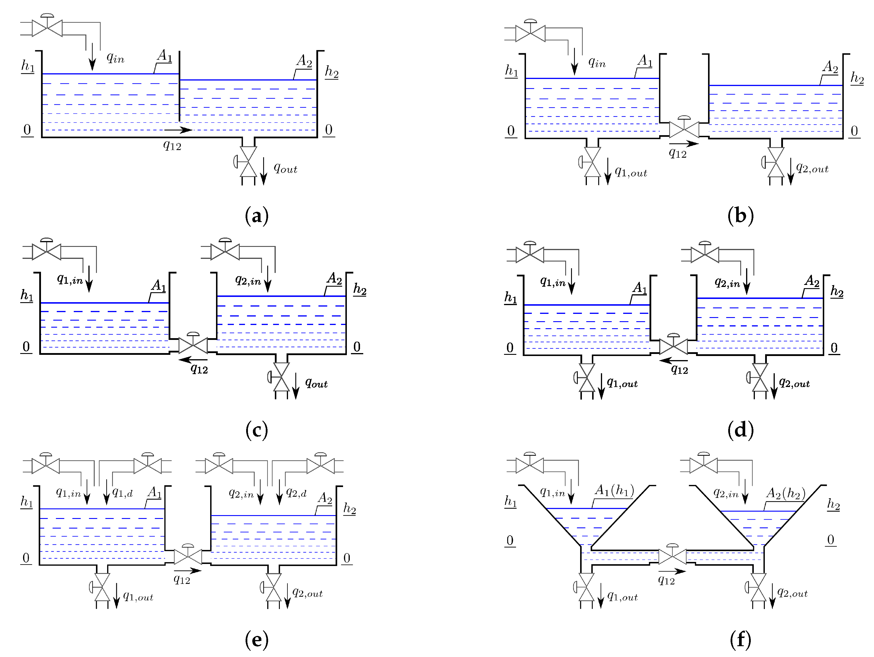
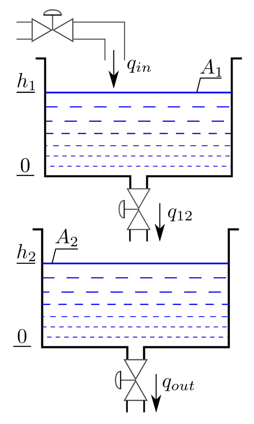
4.2. The Two-Tank Dynamical System

As we have mentioned, the control of water or any liquid level belongs to important industrial processes. Often, they involve two or more interconnected tanks, the levels of which have to be maintained at a reference value, while other levels in the multidimensional space of state may be expected to follow some desired time-varying paths.

Any physical model of the single-tank water level process considered in Section 4.2 can be naturally extended to some coupled or cascaded configurations of two-tank systems schematically represented by two single tanks connected in a series to allow for water flow between them, as is depicted in Figure 2 and Figure 3.

Depending on the physical model, the configurations shown in Figure 2 differ in the presence of inlets to and outlets from the tanks. Referring our survey to some selected but representative research, the coupled two-tank system

(C1)

One control inlet and one outlet; see [36,66] (pump on the outlet), [67] (additional disturbance inflow) [69];

(C2)

One control inlet and two outlets [25,70];

(C3)

Two control inlets and one outlet [30,75];

(C4)

Two control inlets and two outlets [11,12,35,74] (tanks of a conical geometry).

Typically, deriving the basic mathematical model of a coupled two-tank configuration begins with Equations (2) and (3). The volumetric interflow $q_{12}$ m${}^3$/s between both tanks shown in Figure 2a varies accordingly to the difference between the level heights $h_1$ and $h_2$. With respect to that, we obtain:

$$\begin{array}{c}\hfill \frac{d{h}_1\left(t\right)}{dt}=\frac{1}{A_1}\sum _{i_1=1}^{N_1}{q}_{i_1}\left(t\right)=\frac{1}{A_1}\left(q_{in}\left(t\right)-q_{12}\left(t\right)\right),\frac{d{h}_2\left(t\right)}{dt}=\frac{1}{A_2}\sum _{i_2=1}^{N_2}{q}_{i_2}\left(t\right)=\frac{1}{A_2}\left(q_{12}\left(t\right)-q_{out}\left(t\right)\right),\end{array}$$

(15)

where $A_i$ is the constant area of i-th tank, and $N_1$ and $N_2$ denote the number of all flows directed to and from the first and second tank, respectively. In the above mathematical model, the flow $q_{out}$ is defined by Equation (3), since the volumetric interflow

$$q_{12}\left(t\right)=a_{12}\sqrt{2g(h_1\left(t\right)-h_2\left(t\right))}\mathrm{until}{h}_1\left(t\right)\ge h_2\left(t\right),$$

(16)

where $a_{12}$ states the area of the pipe or orifice between the tanks.

The model can be given as a SISO system if the inflow $q_{in}$ stands for the single input to the object, and the level $h_2$ in the second tank stands for the single output from the system. The most frequently used dynamic model of coupled two-tank SISO systems is described by Equation (15), but the volumetric interflow introduced in Equation (16) finds a more general form, which captures the positive and negative differences

$$q_{12}\left(t\right)={\alpha }_{12}\mathrm{sgn}{h}_{12}\left(t\right)\sqrt{|h_{12}\left(t\right)|},\mathrm{for}\mathrm{the}\mathrm{admittance}\mathrm{coefficient}{\alpha }_{12}=a_{12}\sqrt{2g}.$$

(17)

Now, let us continue with the case of linearization of the model. In many realizations, the inflow $q_{in}$ is positive, what means that the pump only supplies the medium to the tank—a charging state occurs. At an equilibrium system’s state, for the constant set-point problem of the level control, the time derivatives of both levels are zero, such that the conditions $d{h}_1/dt=d{h}_2/dt=0$ hold. Applying the conditions to the first of Equations (15), the steady-state equilibrium volumetric inflow $q_{in}=q_{12}$. By analysis of the physical model in Figure 2a, we see that the height $h_2$ will be always less or equal to $h_1$, because there is no additional source of inflow to the second tank that could make its level higher than the level in tank 1, even though the outlet from the tank 2 would be closed. Having this in mind, we return back to the definition in Equation (16). More about modeling, linearization, and operation about equilibrium points and numerical simulations of the types of coupled configurations of tanks (Figure 2a) can be found in [66].

From the other side, if the condition $h_1\ge h_2$ does not hold, if the second tank in the coupled type configuration is supplied with an additional source of inflow (see Figure 2c,e), then the conditioned mathematical model takes into consideration $q_{12}$ defined in Equation (17), and finally, the law of volume conservation in the second tank is governed by the sum of flows ${\sum }_{i_2=1}^{N_2}{q}_{i_2}$ present in the second equation in (15), i.e.,

$$\sum _{i_2=1}^3{q}_{i_2}\left(t\right)=q_{12}\left(t\right)-{\alpha }_2\sqrt{h_2\left(t\right)}+q_{2,in}\left(t\right)\mathrm{for}{\alpha }_2=a_2\sqrt{2g},$$

(18)

and $a_2$ is the second tank’s output orifice area.

More about the mathematical modeling and a real experiment of this type of coupled tanks configuration (Figure 2c,d) can be found in [30,75].

A coupled two-tank system of a conical geometry tanks has been investigated in [74]. The model configuration is similar to the case in Figure 2d, but it is also geometrically conditioned, allowing to us to mathematically describe the height-dependent areas of both coupled tanks.

The cascaded two-tank system presented in Figure 3 is modeled almost exactly as the previously described systems.

It differs in the modeling of the interflow $q_{12}$, since it is not dependent on the difference of level heights in both tanks, but only on the height of level in the preceding tank, i.e., $q_{2,in}=q_{1,out}$, where $q_{1,out}$ is given by Equation (3). If there is not any disturbance inputs, then each tank stands for a single inertial dynamic element. Connecting more elements in a coupled or cascaded series, we find a multi-inertial dynamical system, which is often linearized, as is stated in Section 4.1, and then obtains a higher-order transfer function in the s-domain. Such mathematical representation usually precedes an application of one of the traditional techniques exploiting P, PI, or PID control, as well as its variations, is studied in [11,12,23,25,30,36].

A short conclusion can be drawn. Although other canonical forms of the time-dependent state-space representation of the object of control are present in the theory of control (e.g., a controller, observer or Jordan form), the basic one is still useful, even in two-tank first-order dynamic models.

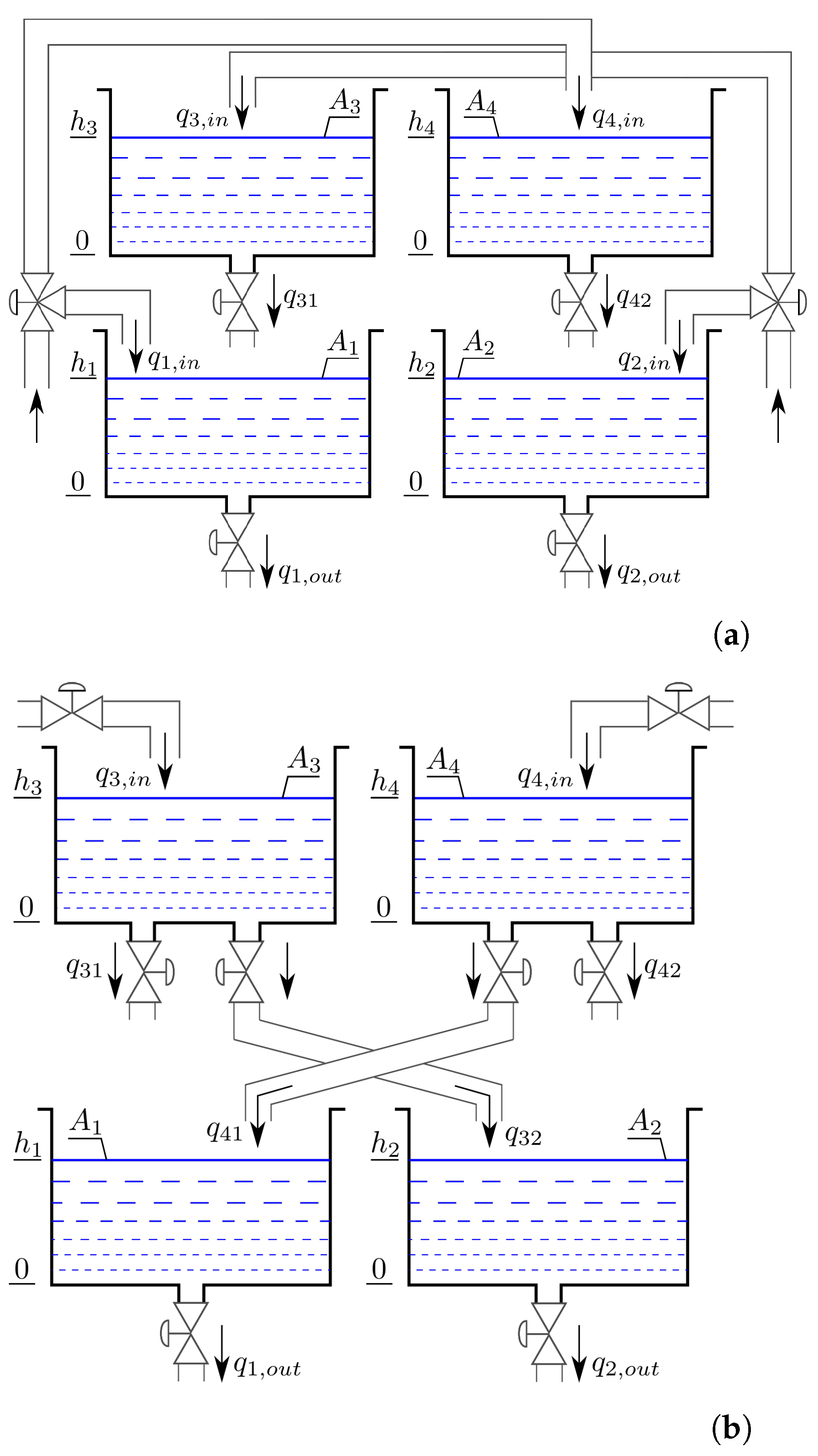
4.3. Multi-Tank Dynamical Systems

Modeling the multi-tank configurations of water level systems, we act in an analogous way. Basing on Section 4.1 and Section 4.2, we add more equations with the definitions of interflows between neighborhood tanks. Therefore, many configurations involving either the pure coupled, cascaded, or their hybrid solutions is developed. Our representative overview of the coupled or cascaded multi-tank dynamical systems refers to the state-space approach, PI and PID, as noted in [8,15,68,77,78,79,80,82,84]; the transfer function approach [10,30,80]; a geometry-varying tank [8,16,79,83]; a dead-time inclusion [80], and a few commonly used control methods, as noted in [14,16] (FL, NN) [9,10,15,78,83] (model-based, model predictive, and state predictor) [77] (SMC).

Many implemented industrial processes have multiple outputs from a single process, what means that they become multi-variable. Thus, the mathematical description and the multi-dimensional control create a more complex dynamical system of many state variables. The controlling technique of such a multi-dimensional process of many state variables is more difficult. In a consequence, a nonlinear triple- or quadruple-tank process is analyzed and controlled in the presence of parametric variations.

An experimental real-time multi-input multi-output (MIMO) nonlinear system composed from three interconnected cylindrical tanks, as shown in Figure 4a, is studied in [15]. Two pumps and six valves were also used, and a reservoir of water was located in the bottom. The water is pumped from the reservoir on the tops of both tanks. The precise positioning of valves and the regulation of efficiency of the pumps is achieved by measuring and controlling the analogue electrical signals. Pressure sensors have been used to measure the heights of all water levels.

The law of volume conservation in the three tanks, governing the dynamics of the system shown in Figure 4a, is based on sums of all flows (compare with Equation (19)), being directed to and from the particular dynamical subsystem, and for j representing the subsequent number of the tank, i.e.,

$$\frac{d{h}_j\left(t\right)}{dt}=\frac{1}{A}\sum _{i_j=1}^{N_j}{q}_{i_j}\left(t\right),\mathrm{for}j=1\cdots 3.$$

(19)

The element-wise summation of all the volumetric flows that charge or discharge each of the tanks of the MIMO dynamical system are expanded as follows:

$$\begin{array}{cc}\hfill \sum _{i_1=1}^{N_1}{q}_{i_1}\left(t\right)=q_{1,in}\left(t\right)-& q_{13}\left(t\right)-q_{1,out},\sum _{i_2=1}^{N_2}{q}_{i_1}\left(t\right)=q_{2,in}\left(t\right)-q_{23}\left(t\right)-q_{2,out},\hfill \\ \hfill & \sum _{i_3=1}^{N_3}{q}_{i_3}\left(t\right)=q_{13}\left(t\right)+q_{23}\left(t\right)-q_{3,out},\hfill \end{array}$$

(20)

where the number of flows is the same for all subsystems, i.e., $N_1=N_2=N_3=3$.

Proceeding in an analogous manner, the mathematical description of the three-tank system with two geometry-varying tanks (see Figure 4b) can be derived; for instance, see [79]. A difference appears, in that some of the tank areas are height-dependent functions of the tank geometries according to the algebraic formulas:

$$A_1\left(h_1\right)=vw,A_2\left(h_2\right)=\frac{bw}{H_{max}}{h}_2+cw,A_3\left(h_3\right)=w\sqrt{R^2-{(R-h_3)}^2},$$

(21)

where the area $A_1$ is not dependent on $h_1$, and the geometric constants b, c, v, w, and R depend on the dimensions of all the tanks.

Figure 5, together with the representative literature referenced in the caption, presents other interesting hybrid configurations of quadruple-tank systems that are subjected to the same rules of the mathematical model’s derivation, as is based on Equation (20).

One should note that in the case of the cascaded part of a serial connection of tanks, the sgn function, as written in Equation (17), which captures the positive and negative differences of liquid levels in the vertically adjacent tanks, has to be considered.

At the end of this section, we reach a brief summary. Due to the almost constant density of water, the mass conservation law is less frequently used in the derivation of the mathematical models of water-tank systems in favor of the volume conservation law. The mathematical models, especially those of multi-tank dynamical systems, could be given in a much compact—general mathematical form, as is introduced by Equation (19). Although our review of the literature extends on many references, we have not reported any name for the flows between subsequent tanks, so the term of a volumetric interflow has been adapted. Beginning from a single- to multi-tank systems, the mathematical models have been generalized in the same name space of the variables, allowing the reader to compare their structural complexity, which synthesizes the knowledge and can also be helpful in any further investigations of the water level control problems of applied mechanics. A deeper study of the literature, being referenced to in this section, shows that the mathematical models of the SISO or MIMO dynamical systems serve as a background to an application of various control strategies presented in the next section.

5. Model Analysis and Control Strategies

5.1. Traditional Approaches with Modern Inclusions

The traditional design of the so-called control laws bases on the well-known P, PI or PID controllers—a family of very simple mathematical operations in the continuous or discrete time domain [2,25,26,36,39,67]. This approach is good enough for solving most problems of water level regulation in a single- or two-tank systems, but may be insufficient while searching for the fast and robust control of level in multi-dimensional water tank systems.

A modern inclusion to the traditional control approaches is shown in [7], where an overview of the P and PI control of the liquid level in a nonlinear single-tank system associated with exact linearization is performed. The authors have modified it using the consideration of not modeled dynamics and a nonlinear disturbance-observer that is based on integral action as well. According to the nomenclature introduced by the authors, the assignments in the cited work use two paradigms, i.e., the learning by doing and the learning by experimenting carried out in a quasi-real laboratory model of a CTS.

Proportional or proportional-integral controllers play a crucial role in the regulation of liquid level. In paper [61], an averaging level control is considered. The reduction of flow variations at liquid levels varying in time was the main difficulty in the solution of the problem of control. We meet here another problem such as the overfilling and full emptying of the tank. To avoid the unpredictable behaviors, the liquid level has to be operated in the frame of the assumed safety constraints. The authors of the work propose a simple PI scheme for the usual operation and two P controllers of a high gain, maintaining the liquid level in the constraints. At the end, less effort of modeling and a smaller time of computations at a simpler tuning of the controller have been obtained in the introduced MPC strategy.

Following paper [15], a simple design and a satisfactory level of efficiency of the conventional PID controller mainly decides its popularity in mechanical engineering, andoverall, in industrial applications. As usual, there is no golden solution to every application, since the parameters of the PID controller have to be particularly set to achieve the desired efficiency of a set-point or even a smooth reference signal tracking regulation. With respect to that sometimes challenging task, many experimental works in the last decades have been oriented on providing some methodologies or algorithms of tuning of PID controllers for the linear time invariant dynamical systems.

A discretization-based auto-tuned PID MPC is proposed in [15] on the basis of the control of nonlinear systems in the continuous time domain. The tuning of the PID controller is made in a parameter prediction scheme, delivering an enhanced degree of tuning that is based on the minimization of the square of error of the regulation. It belongs to the MPC approach, which provides an adaptation of the controller’s parameters at a simultaneous generation of additive terms correcting the controller’s parameters. Finally, experimental real-time systems serve as the models of testing of efficiency for the proposed methodology.

The controllers of a simple form are still explored, but an estimation of their gains and time constants is carried out using genetic algorithms [19]. The controller is tuned online by GA—a genetic algorithm that is a method of stochastic global search. In the innovative method, one operates on a set of potential solutions. The principle of survival of the well-fitting candidate to the solution found after some evolutions is applied. With regard to some limitations of the water tank system presented, it was difficult to achieve the most optimal control of water level with the use of only constant parameters of the PID controller. Therefore, they had to be changing in time. Due to that, the strategy of online tuning of the generic algorithm is included. The introduced GA locates areas of high performance without the difficulties, appearing in high dimensional systems or even false optima, and occurring in the methods of gradient decent.

A VS PI controller characterized by a variable structure for the process of level control is proposed in [60]. An analysis of the performance and stability of the system is analyzed by the authors with the use of a describing function method. They show that the improved controller makes the dynamical system a quasi-linear one. In comparison to the conventional PI controller, the properly tuned VS PI controller provides higher performance.

An assessment of the very important feature is a crucial consideration to underline in the literature devoted to liquid level control. The nonlinear process conducted in [65] has been expressed in terms of a transfer function approach. It has allowed for a better PID control of the water level, the parameters of which have been optimized with the use of a PSO. The authors have achieved in the simulations an effective set-point control and also the tracking of a level along a reference trajectory. The reader can find in this work an overview of adaptive controllers and PSO.

As is observed in [11], the level in one tank has to be kept at a constant value, but the level in the other is required to track a reference signal varying in time. In such cases, the traditional PID solution in a feedforward realization of the controller will not be capable of rejecting the disturbance, having appeared after a change of level in the second tank, and consequently, to keep the level in the first tank at a constant value. Normally, such a disability causes a decrease of the tracking performance of the water level in the second tank. This is a very interesting observation, proving that even in such two-dimensional cases, the golden PID controller may be insufficient. Based on analytic and experimental investigations, the authors propose the usage of a FOPI—a fractional order PI controller to be designed in the frequency domain. The performance of the controller is tested on an experimental setup, where a constant level was maintained in the first tank, but the level in the second tank followed some periodic reference test signals. More about modern inclusions to the traditional controller design can be found in Section 5.3, which we dedicate to the MPC (model-predictive control).

5.2. Experimental Identification and the Estimation of Model Parameters

One of the methodologies allowing the designer of any control system to deal with a large number of requirements that the system has to satisfy is to engage the experimental data that have been obtained by forcing the object of control to perform a measurement of its response. This approach is covered by an interdisciplinary identification of dynamical systems. For instance, we use the identification of parameters if the object of control is structurally complex and could be provoked by a strong nonlinearities, affecting the dynamics of the physical model of the object.

The literature of recent years presents a kind of translation of the identification methods between the linear and nonlinear systems [86,87]. In this context, the necessity of capturing of the inherent nonlinear phenomena governing the real systems’ dynamics is crucial. As we have observed and written in Section 6, treating about the experimental part of our review, an identification of the nonlinear system faces the challenge of the flexibility of the estimated model and its ease of mathematical description at once.

In a reference to [17], there is not any general methodology of the identification of real nonlinear systems, the modeling of which are covered by either statistical or machine learning. We find in the reference that most of these methods are not fully oriented on the dynamics due to limited means for dealing with measurement noise. A methodology showcased in the work identifies a flexible NLSS model—an unstructured flexible nonlinear state-space model for the water CTS, on the basis of a cascaded water-tank identification problem.

In a view of the announced engineering problem, the contribution [72] addresses the identification of different flexible structures of nonlinear systems with soft and hard nonlinearities in the cascaded water tanks identification problem as well. Beginning from the simplest structures of linear black box models, the authors extend the scope of their studies on the nonlinear ones and compare them by investigating a series of models with increasing complexity, based on a prior knowledge of physics. It is shown that while the linear models are well in prediction, a better description of the nonlinear effects is needed to achieve a good performance in numerical simulations. The contribution even brings an overview of real identification problems.

At the end of this section, let us mention the noteworthy paper [5], which proposes an identification of a water level dynamical system made with the use of both NN and FL, i.e., the neurofuzzy approach. In this study, a water level dynamical system is analyzed using an adaptive ANFIS—a network-based fuzzy logic inference system. The model is applied to develop and to use a PI control. The application of a real system and the ANFIS model produce interesting results that are finally discussed and compared with respect to the identified system efficiency.

5.3. Model Prediction

The future dynamical behavior of an object can be forecast (predicted) using the MPC—model-predictive control, in which optimal decisions are conditioned via an optimization algorithm. This feature has been utilized the autonomous control of water level systems for the purpose of the trajectory tracking problems, where the future reference is included to improve the control performance. Such a treatment opens the control algorithm for an adoption of future errors of regulation.

Every sampling instant of a discrete model is used to solve the optimization problem in an NGMPC—a nonlinear generalized model-predictive control presented in [9], to compare with the NMPC studied in [35]. The implementation has to be repeated on the object in RT. Therefore, with respect to the computational complexity, an analytic solution to the NGMPC problem is approximated by Taylor expansion from the tracking error and the effort of control. Thanks to that, omitting the online optimization, the controller could have been formulated in a closed form.

Making a short enumeration of recent advances in this field, the methods engaging the MPC were developed within the project HD-MPC [88]. Decentralized strategies of control were studied in [10] using five methodologies that were based on a distributed multi-parametric model-predictive control. The same type of controller was explored in [89], but this time, a linearized state-space model was proposed. Another distributed and even hierarchical MPC with fast gradient-based optimization was investigated in [90], since a nonlinear generalization of this type of control takes into consideration a back-stepping algorithm in [91].

Any linear model approximation of nonlinear systems introduces a non-modeled part of dynamics and the uncertainty of parameters of the mathematical (physical) model. As a result, a steady-state error appears and the actual response of the water level system exhibits an uncorrectable error of regulation. We can cope with the inaccurateness by placing an integral action in the closed-loop control system. Such an approach, allowing for an increase in the robustness of a controlled CTS, has been used in [37]. A wireless MPC of a water level was implemented by the authors. They stated the objectives of the optimization, and the level was maintained within a range of a set of pre-defined values. To prove the effectiveness of the wireless model-predictive control, the authors conducted a real-time simulation of the MPC algorithm, including the integral action.

A special field of applications of control strategies is lately reserved via distributed control. Multi-parametric quadratic programming-based controllers are developed in [10] for a quadruple-tank problem. The stable and optimal operation of the developed decentralized control in some superposed constraints requires the use of a distributed MPC extended on game theory. Similarly to the previous reference, the integral action in a form of the PI controller has been introduced to improve the reference signal tracking and rejection of disturbance. Another quadruple-tank control problem tending to meet similar requirements has been solved in [78].

5.4. Time Effects

Measurement procedures, communication lags, computational processing, or even many processes of a media transportation are subjected to time delays. Big delays cause the instability of control algorithms, because the controller’s responses are highly inappropriate to the current dynamical behavior of the plant. For instance, the opening or closing of valves being an alternating input to the system makes the problem more difficult. Robust control is of main interest for almost all strategies. With respect to that, a dynamical behavior of each closed-loop system should be satisfactorily well-resistant to small parameter perturbations, measurement noise, and also at the time delay, remaining in acceptable bounds. In scope of that, the robust MPC shortly overviewed in Section 5.3 may be of particular interest, if the enforcement of some constraints for th eoperation of an actuator or process variable is mandatory.

An exemplary work, considering the problem of time delays in a predictive control, is conducted in [22]. The robustness of the response of a two-tank system with time delays and input constraints has been achieved by representing the time delay uncertainty in a polytopic form and by using the linear matrix inequalities.

At the end of this subsection, we only signalize the problem of dead time that was investigated, e.g., in [80], on the basis of a novel quadruple-tank multi-variable control process, incorporating independent multi-variable dead-time zones.

5.5. Sliding Mode Control

The control systems of variable structures play an important role in the nonlinear dynamics. The SMC—sliding mode control, belongs to the branch of algorithms that control the nonlinear dynamical systems, applying a very fast time-discontinuous switching on a predetermined surface of sliding. The SMC, operating usually with a nonlinear feedback, is composed of a sliding surface that is found for a desired stable dynamics, and also of the control algorithm, which excites dynamics of the considered object of control to reach this sliding surface and to stay on it as long as it is possible. In the sliding surface’s reaching mode, th etrajectories of the dynamical system are sensitive to fluctuations of model parameters, as well as to disturbances, but they are not sensitive, being in the sliding mode. Although the transient state is subject to the aforementioned variations, the SMC’s discontinuous nature of action is highly robust in the output tracking problem and for the stabilization of the system. As a consequence, an insensitivity of the obtained control performance to variations of parameters and the rejection of disturbances is reported. From the point of view of application of the methodology of a variable structure control of liquid level, some achievements can be pointed out in the literature mentioned below.

An exemplary application of one degree SMC (1-DoF SMC) used in [66] is to control the height of water level in a numerical model of the CTS, using an integral variation of the method, which reduces the chattering problem. The relative degree of the sliding variable is equal to one, since the asymptotic stability of the closed-loop control system is guaranteed. The simulation results presented by the authors indicate that the proposed control technique is characterized by good performance, as proven by the time histories of water level changes in the tanks. Other curious attempts in this field devoted to a neuro-fuzzy approach with a nonlinear sliding surface [92], or a sliding surface parameter, depending on the state [93] can be mentioned.

The 1-DoF SMC has a disadvantage, because the high frequency of switching around the sliding surface produces chattering. An elimination of this effect can be achieved in higher-order realizations. One is able to read about some interesting studies of water level control, using the second- and higher-order sliding mode control in [75,76,84], where, respectively: the derivative of the sliding variable is not necessary, less information about the CTS system is required in comparison to 1-DoF SMC, and the conventional sliding surface applied to a quadruple-tank system is altered with the dynamics of fractional order.

Concluding this part of the overview, beginning from the SMC methods and its variations, the multi-dimensional water level control problem has become more complex, but mostly more effective. Another successful attempt for solving the multi-tank problem continues this tendency via the application of the PSO and NN [5,6,16,35,63,65], since the most popular FL control is described below.

5.6. Fuzzy Logic Control

As we have noted, the previously described methodology is associated with a big chattering of control. The experiments conducted in the last decade have demonstrated that a fuzzy controller with adaptation abilities can be successively applied to the not necessarily well-defined or even completely not available dynamical system [94]. In addition, the AFC—adaptive FL control, proves its specific features to enhance the robustness of the nonlinear control problems. For instance, comparing the AFC with the conventional PI, the first one presents a better tracking performance, while the transient responses of the object of control bring a shorter time of settling and also a smaller overshoot (undershoot) of the responses. Moreover, a much more robust control with respect to the disturbance-caused fluctuations of water level is reported.

A PDC—parallel distributed compensation method, states a background in [62] for a FL controller implemented to an experimental setup of water level control.

As in our experimental test setup described in Section 6, the mathematical model is identified experimentally based on estimations of system responses. The control of height of water level is realized in the full range of changes of the level that is achieved via the linearization of the nonlinear model around a set of the assumed operating points. Using a fuzzy blending of the PI controllers, working at the specific operating points, the PDC-based FL controller has been designed. It turns out that the controller is better than the reference PI controller, based on the FL approach as well. More about the PDC methods can be found in a short literature overview included in the cited paper.

The authors of paper [70] propose the so-called FM—fuzzy-molecular method to robustly control the water level in a CTS with variable rates of volume discharge at the second tank. In view of an application of a hybrid FL inference system and the defuzzification performed with the use of artificial hydrocarbon networks, they propose the FM controller as the one properly dealing with noise and the uncertainty of dynamics around the operating points. It is curious, but the experiments have proven that a knowledge of the model of the plant is not necessary.

Other linked applications of water level control refer to, e.g., the implementation of a computer-embedded FL controller [3], interval FL controller of second type for a two- [71] and three-tank system [14], Cuckoo optimization algorithm [20], simultaneous FL- and PID control in LabVIEW [26], stiction compensated FL controller design for a nonlinear spherical tank level system using LabVIEW [27], and a fuzzy dynamic parameter adaptation in ant colony adaptation and PSO applied to the regulation of water level [65].

Although they might look quite advanced, most of the techniques developed or explored in the examined field of control of the analyzed process are adopted from the general theory of modern control. Special treatment appears on the level of identification of the parameters and the static characteristics of the investigated systems of water level control (see also Section 2.2 and Section 6).

5.7. Special Approaches

Let us enumerate some dedicated approaches, the specific applications of which are present in the related literature, e.g.: (i) a model reference control driven from the experimental data of MIMO cascaded tank systems, including the tuning of a virtual reference feedback [83]; (ii) nonlinear control of a three-tank CTS with mismatched uncertainties [79]; (iii) a robust high-gain observers-based water level and leakage flow rate estimation [77]; (iv) the control of two conical tanks with interacting levels based on a dynamic matrix approach [74]; (v) a Volterra series estimate of the CTS using multidimensional regularization [73]; (vi) black and white box approaches for a CTS identification [72]; and (vii) a few references [8,12,18] described in Section 2.

At the end, let us briefly summarize Section 5. Although our overview takes into consideration the contributions of the last decade, the authors of many of them refer to older literature references, trying to incrementally improve either the existing mathematical modeling, the identification approaches, or the control strategies. Of course, reported in our survey are plenty of innovative theoretical or experimental approaches to the identification, maintenance, and regulation of various liquid level control systems. The technique based on the FL approach looks as the most widely explored one in the domain of liquid level control, as well as the identification or tuning of model parameters, but the well-established methodologies involving the classical theory of linear and nonlinear control are still alive in an improved form.

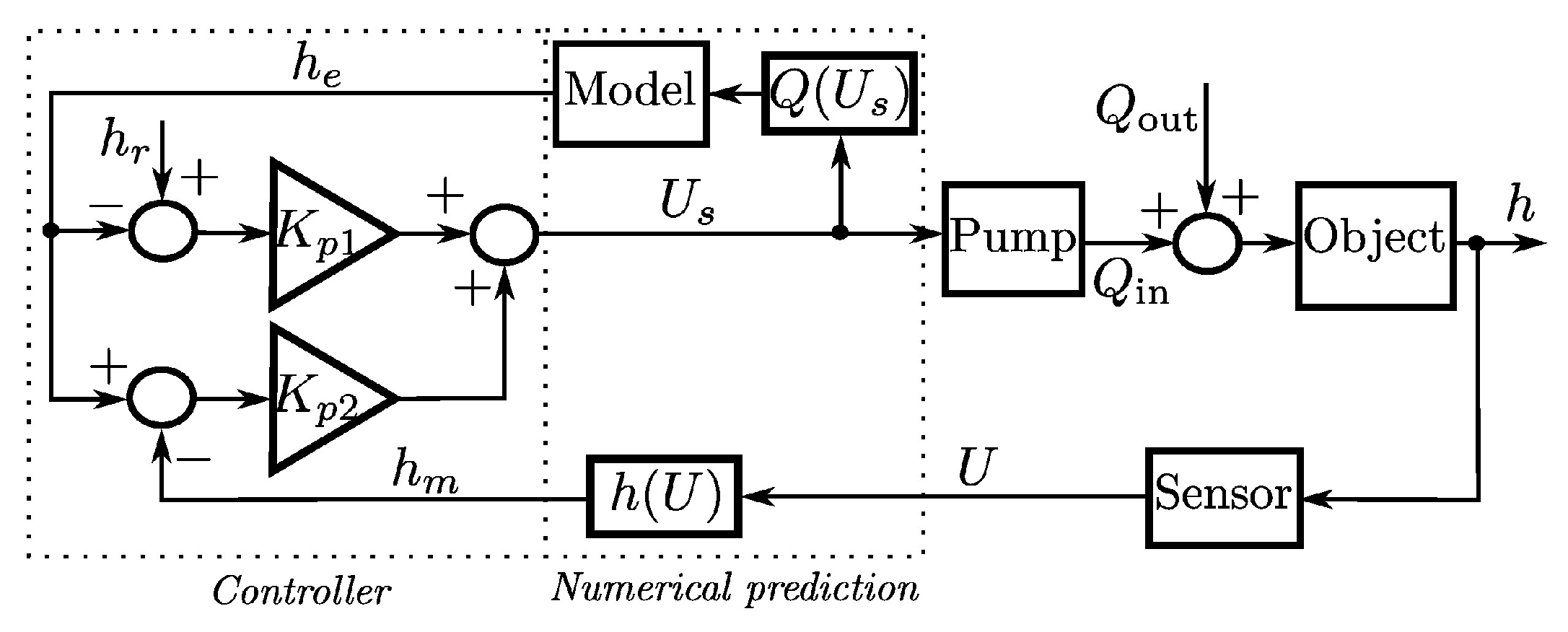
6. Proportional Control with Correction Based on a Numerical Prediction of Water Level

A tank or any system of connected or even cascaded tanks with water under atmospheric pressure and negligible temperature fluctuations should be considered as a simple control object, requiring the simplest possible level control system. In this way, we concentrate on searching for the simplest but most effective control strategy supported by the numerical model. More about the construction and mechatronic devices can be found in [95].

As in Section 4.1, we analyze our control object that is understood as a linear differential model—an integral dynamic element. It holds because the associated level control system has to deal with the nonlinear characteristics of inputs and outputs, and flow resistance, all of which are inaccuracies of physical and mathematical modeling, but they must also must eliminate any measurement noise. The mathematical modeling of our dynamical system is simply governed by the mathematical model given in Equation (13).

A concept of a new experimental setup shown in Figure 6 serves for a precise control of water level in the modern single-tank-reservoir system.

Adjusting the set point in the event of disturbances in the water volume and checking the step response of the pyramid-shaped system is preceded by the identification of the system parameters. These include the pump efficiency and the resistance of water outflow from the tank. In the next step, sequential hybrid proportional closed-loop control is applied with correction based on a numerical prediction of the state of the system and the actual measurement of the state of the system to map successive states of the water level. The mathematical model given by Equation (13) of the two configurations of the tested hydraulic control system was developed using LabVIEW virtual instruments.

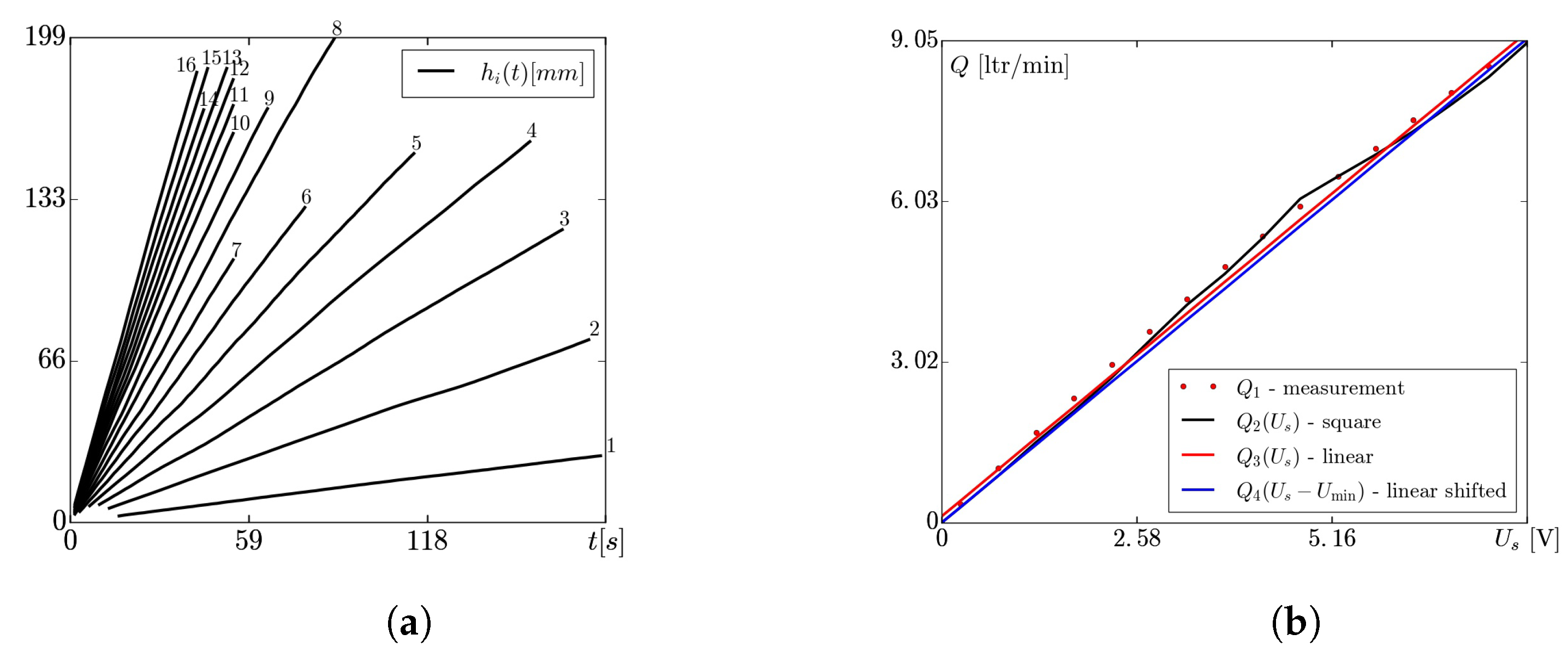
6.1. Identification of the Hydraulic System

Identification of the pump performance from 16 static characteristics $h_i\left(t\right)$ for $i=1\cdots 16$ of the tank filling at constant voltage values $U_i$ applied to obtain 16 increasing rates of pumping of the peristaltic pump results in the linear characteristics shown in Figure 7a.

The coefficients of the characteristics have been approximated and presented by red dots in Figure 7b, which shows a comparison of the square and linear approximations of the real volumetric efficiency of the peristaltic machine against the measured values.

The linear mass flow rate ${\tilde{q}}_{in}\left(U_s\right)=0.0193U_s-0.0046$ at the input depends on the control voltage $U_s$ in the allowed range of 0.25-9 V. An estimation of the outflow resistance of the observed laminar flow, i.e., $R_l\left(h\right)=-6867h^2+99619h$, captures the irregularities of the inner shapes of the hydraulic armature. The resistance was estimated according to Equation (7) after a series of measurements of the level and the corresponding outflow. Finally, the water level dependency on the sensor’s voltage U is found in the form $h_m\left(U\right)=0.0556(U-U_0)$, where $U_0$ is the reference initial reading at $h_m=h_{m,0}$.

Figure 8 shows a closed-loop control system with two proportional controllers, and a correction based on the prediction of the numerical state variable.

The most useful feature of the control system is that the pump control input, coming from the numerical prediction, is found from a smooth numerical estimation of the water level in the tank. It guarantees a better robustness of the system and stability of regulation.

It has turned out that the precisely estimated characteristics of pump efficiency and also the laminar outflow resistance are dependent on the temperature of water, and on the temperature and pressure of air in the space surrounding the test setup. With respect to that circumstances, the two non-dimensional coefficients: $c_1$—responsible for correction of inflow filling the tank, $c_2$—responsible for the correction of outflow resistance during the emptying of the tank (see the corresponding slopes in Figure 9), both positive and less than 1, have to be identified at the initial stage of the process of regulation. Both constants have to be adjusted until the black line of the numerical solution will be coinciding with the red line representing the measurement. Usually, the automated calibration process takes about 30 s.

Correction of the mass inflow ${\tilde{q}}_{in}$ enforces multiplication by $c_1$, while the correction of the mass outflow ${\tilde{q}}_{out}$ requires a similar multiplication by $c_2$.

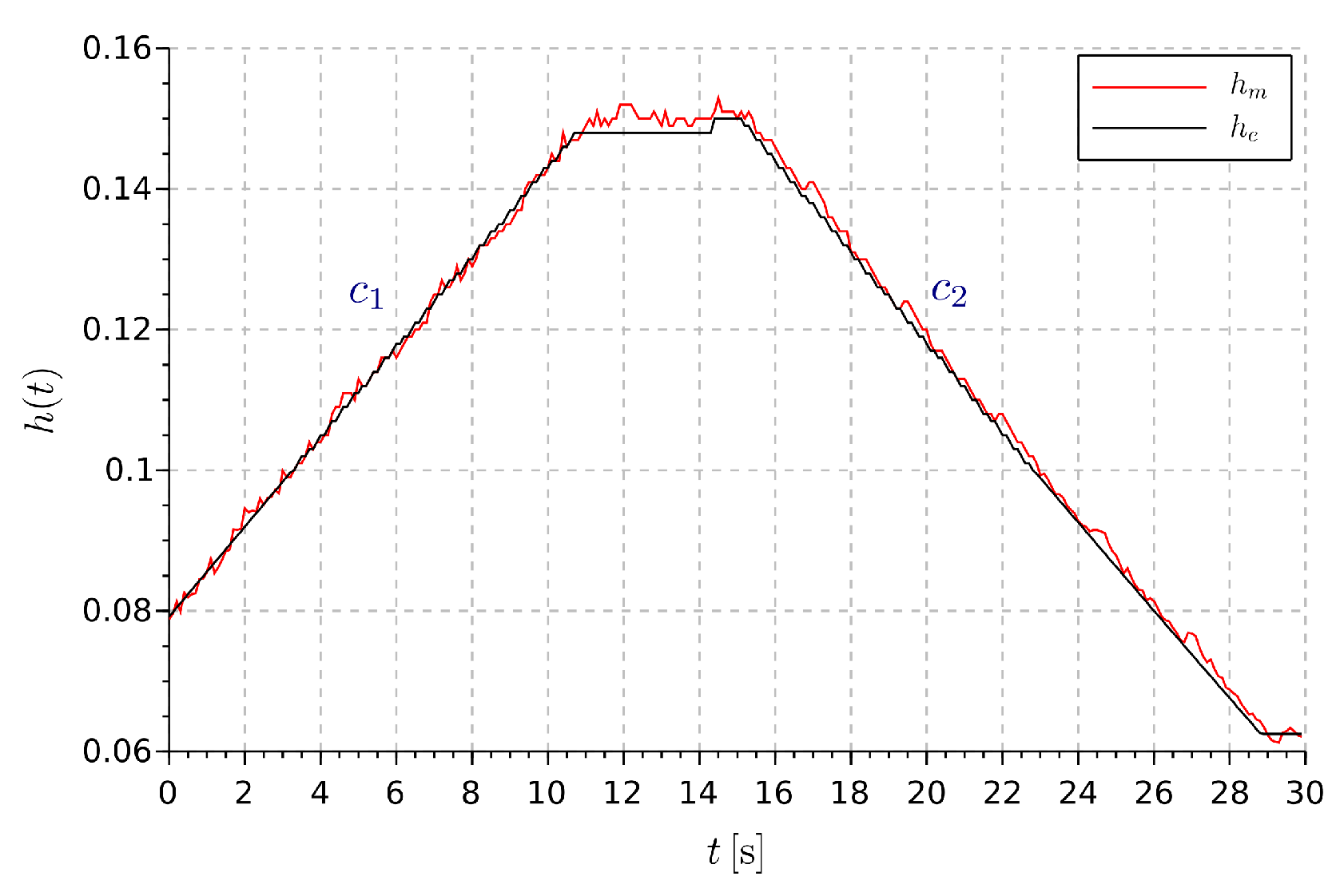
6.2. Control of the Experimental Test Station

In the further part of the description of this experiment, we will base on the previously made idealization of the actual test stand and the tank with outflow, inflow, and disturbance implemented there. Our goal will be to apply a numerical prediction, obtain the intended step function of $h_m$, and keep this response as close as possible to the reference function $h_r$, using a numerical estimation $h_e$ approximating a series of measured values $h_m$.

The superiority of the hybrid proportional closed-loop control with numerical prediction is confirmed after comparing the time histories shown in Figure 10; see more broadly in [95]. It is important to note that during the experiments, the same parameters of the precisely identified experimental model were used.

The experimental verification of the effectiveness of the proposed two-stage P hybrid control system with numerical prediction of the water level, as shown in Figure 10, is finally investigated on the basis of a new form of the test signal—a pyramid-shaped test reference input determined by an amplitude-modulated step function matched by a green line. It is built from a series of reference set-point inputs, $h_{r,i}=\{2,6,10,14,10,6,2\}\times {10}^{-2}$, for $i=1\cdots 7$. After four step responses of the system for the increasing amplitude, reaching the highest reference value at $h_{r,4}$, the pump stops working, and at $t=65$ s, the solenoid valve starts to properly open the system’s outlet for a time, allowing for gravitational flow of the water out of the tank and for the new decreasing set-point value to be reached. The final reference level $h_{r,7}$ is achieved after the third closing of the valve at about $t=125$ s. After that full cycle, the actual value of the level can be referenced to the final step input to measure the error of regulation.

Making an assessment of the convergence of the observed system responses registered in the final test of efficiency of the designed 2-stage P controller with numerical prediction, the numerically estimated level mostly follows the pyramid-shaped discontinuous reference input very well. This is because its real adequate proves its proper convergence, as shown in Figure 10b, for $k_p=400$, where after the occurrence of an overshoot of the level height at $t=110$, and after the last switching of the valve, the level stabilizes on the last reference $h_{r,7}$, aswas required.

Summarizing this section, the basic but improved control system design with numerical prediction of the real state of the system and also real measurement readings, provide a good control effect. Numerical prediction makes it possible to more effectively reject the sensor’s measurement noise and to stabilize the actual water level in the tank at the desired value.

7. Conclusions

In spite of the rapid development of mathematical analysis applied to the control of water level systems, there has not been such a broad overview devoted to the field of dynamical systems and its control that has been made in the current literature. This contribution aims at complementing this gap by performing a systematized and concise overview of the intelligent mechatronic systems used in the measurement, identification, and control of water level. Making a reference in the concluding part of the paper to some particular sections, the following general observations are made.

MATLAB/Simulink and LabVIEW are the most commonly exploited environments in the modeling of dynamical systems conjugated with the design of virtually realized control systems.

Each of the modern techniques and sensors for water level measurement and control has its own dedicated realizations, the features of which are used in some specific or more general realizations of detection and the monitoring of filling level. A common feature of the newest achievements in this field is distinguishable in the exploitation of modern material and electrical engineering. Miniaturization, introduced along with the popularization of microcontrollers, allows us to embed more or less sophisticated mathematical algorithms. The very expanding use of microelectronics makes the mechatronic measurement systems more applicable, realizable, and intelligent.

The mass conservation law in mathematical modeling is less frequently used in the derivation of mathematical models of water-tank systems in favor of the volume conservation law. The mathematical models, especially those of multi-tank dynamical systems, could be given in a much compact mathematical form. Beginning from a single- to multi-tank systems, the mathematical models have been generalized in our work in the same name space of the variables, allowing the reader to compare their structural complexity, which synthesizes the knowledge and can also be helpful in any further iterate investigations of the water level control problems of applied mechanics and mechatronics. Uniformed pictures of coupled or cascaded tanks configurations may also be helpful in this matter.

The authors of many contributions of the last decade refer in their studies to older literature references, trying to incrementally improve the system modeling, identification approaches, or control strategies. There are plenty of innovative theoretical or experimental approaches to the identification, maintenance, and regulation of miscellaneous water level control systems reported in our survey.

The technique based on the fuzzy logic approach looks like the most explored technique in the domain of liquid level control, as well as in the identification or tuning of model parameters, but the well-established methodologies of the classical theory of linear and nonlinear control are still present in an improved form.

The new term, volumetric interflow, which up to now does not exist in the literature, devoted to the control of water-tank processes, is introduced, whilst its use is justified in the description of various types of flow between the surge, reservoir, or process tanks.

A new test is proposed, engaging a pyramid-shaped step function, having a form of the discontinuous path of reference level, and also engaging the operation of the pump and the valve on the outlet separately to check the efficiency of the designed control system in both directions, i.e., during the filling and emptying of the tank.

More extensive research on the control methodology to be applied at the presented experimental station, including the development of its design and deeper mathematical analysis, will be undertaken in a prospective work, where more methods will be applied, including PID, FL, and differential evolution.

References

1. Kunikowski, W.; Czerwiński, E.; Olejnik, P.; Awrejcewicz, J. An Overview of ATmega AVR Microcontrollers Used in Scientific Research and Industrial Applications. Pomiary Autom. Robot. 2015, 215, 15–20. [Google Scholar] [CrossRef] [Green Version]
2. Mamur, H.; Atacak, I.; Korkmaz, F.; Bhuiyan, M. Modelling and Application of a Computer-Controlled Liquid Level Tank System. In Proceedings of the Seventh International Conference on Computer Science, Engineering and Applications (CCSEA-2017), Dubai, UAE, 28–29 January 2017. [Google Scholar] [CrossRef]
3. Krivic, S.; Hujdur, M.; Mrzic, A.; Konjicija, S. Design and implementation of fuzzy controller on embedded computer for water level control. In Proceedings of the MIPRO, 2012 Proceedings of the 35th International Convention, Opatija, Croatia, 21–25 May 2012; pp. 1747–1751.
4. Omijeh, B.; Ehikhamenle, M.; Elechi, P. Simulated Design of Water Level Control System. Comput. Eng. Intell. Syst. 2015, 6, 30–40. [Google Scholar]
5. Turki, M.; Bouzaida, S.; Sakly, A. Identification of a water level system using ANFIS. In Proceedings of the Proceedings Engineering and Technology, International Conference on Control, Engineering and Information Technology (CEIT’13), Tlemcen, Algeria, 25–27 May 2014; Volume 3. [Google Scholar]
6. Turki, M.; Sakly, A. Modelling of water level system using neurofuzzy tuned by PSO. In Proceedings of the 17th International Conference on Sciences and Techniques of Automatic Control and Computer Engineering—STA’2016, Sousse, Tunisia, 19–21 December 2016; pp. 54–60. [Google Scholar] [CrossRef]
7. Tapak, P. Nonlinear Control of Liquid Level. IFAC Proc. Vol. 2012, 45, 218–223. [Google Scholar] [CrossRef]
8. Rosinova, D.; Balko, P.; Puleva, T. Teaching multiloop control of nonlinear system: Three tanks case study. IFAC-PapersOnLine 2016, 49, 360–365. [Google Scholar] [CrossRef]
9. Gouta, H.; Said, S.; Barhoumi, N.; Faouzi, M. Generalized predictive control for a coupled four tank MIMO system using a continuous-discrete time observer. ISA Trans. 2016, 67, 280–292. [Google Scholar] [CrossRef] [PubMed]
10. Velswamy, K. Distributed multiparametric model predictive control design for a quadruple tank process. Measurement 2013, 47, 841–854. [Google Scholar] [CrossRef]
11. Roy, P.; Roy, B. Fractional Order PI Control Applied to Level Control in Coupled Two Tank MIMO System with Experimental Validation. Control Eng. Pract. 2016, 48, 119–135. [Google Scholar] [CrossRef]
12. Dulau, M.; Dulău, T.M. Multivariable System with Level Control. Procedia Technol. 2016, 22, 614–622. [Google Scholar] [CrossRef] [Green Version]
13. Terzic, E.; Nagarajah, R.; Alamgir, M. Capacitive sensor-based fluid level measurement in a dynamic environment using neural network. Eng. Appl. Artif. Intell. 2010, 23, 614–619. [Google Scholar] [CrossRef]
14. Sahu, H.; Ayyagari, R. Interval Fuzzy Type-II Controller for the Level Control of a Three Tank System. IFAC-PapersOnLine 2016, 49, 561–566. [Google Scholar] [CrossRef]
15. Cetin, M.; Iplikci, S. A novel auto-tuning PID control mechanism for nonlinear systems. ISA Trans. 2015, 58, 292–308. [Google Scholar] [CrossRef] [PubMed]
16. Belikov, J.; Petlenkov, E. Model based control of a water tank system. IFAC Proc. Vol. 2014, 47, 10838–10843. [Google Scholar] [CrossRef] [Green Version]
17. Relan, R.; Tiels, K.; Marconato, A.; Schoukens, J. An Unstructured Flexible Nonlinear Model for the Cascaded Water-tanks Benchmark. IFAC-PapersOnLine 2017, 50, 452–457. [Google Scholar] [CrossRef]
18. Perez-Correa, J.; Lefranc, G.; Fernandez-Fernandez, M. A New Application of the Hill Repressor Function: Automatic Control of a Conic Tank Level and Local Stability Analysis. Math. Probl. Eng. 2015, 2015, 1–6. [Google Scholar] [CrossRef] [Green Version]
19. Aljumaili, M.; Koh, S.; Chong, K.; Tiong, S.; Obaid, Z. Genetic Algorithm Tuning Based PID Controller for Liquid-Level Tank System. In Proceedings of the International Conference on Man-Machine Systems (ICoMMS), Pulau Pinang, Malaysia, 26–27 August 2009. [Google Scholar]
20. Balochian, S.; Ebrahimi, E. Parameter Optimization via Cuckoo Optimization Algorithm of Fuzzy Controller for Liquid Level Control. J. Eng. 2013, 2013, 982354. [Google Scholar] [CrossRef]
21. Mustapha Imam, A.; Tijjani, Y. PLC-Based Water Level Control. Afr. J. Sci. Res. 2016, 5, 65–67. [Google Scholar]
22. Rossi, F.; Galvao, R. Robust Predictive Control of Water Level in an Experimental Pilot Plant with Uncertain Input Delay. Math. Probl. Eng. 2014, 2014, 1–10. [Google Scholar] [CrossRef] [Green Version]
23. Tomera, M. Comparison analysis of three PID-type algorithms: Linear, fuzzy, neural. Automatyka Elektryka Zakłócenia 2011, 6, 1–19. [Google Scholar]
24. Larsen, R.W. LabVIEW for Engineers; Prentice Hall: Hoboken, NJ, USA, 2011. [Google Scholar]
25. Bastida, H.; Ponce, P.; Ramirez-Mendoza, R.A.; Molina, A. Model and Control for Coupled Tanks Using Labview. In Proceedings of the IEEE 2013 International Conference on Mechatronics, Electronics and Automotive Engineering (ICMEAE), Morelos, Mexico, 19–22 November 2013. [Google Scholar] [CrossRef]
26. Sabri, L.; Al-mshat, H. Implementation of Fuzzy and PID Controller to Water Level System using LabView. Int. J. Comput. Appl. 2015, 116, 6–10. [Google Scholar] [CrossRef]
27. Meenatchi Sundaram, S.; Purohit, A. Stiction Compensated Fuzzy Controller Design For Non Linear Spherical Tank Level System Using Labview. Int. J. Pure Appl. Math. 2018, 20, 2023–2031. [Google Scholar]
28. Vasistha, V. Remote Access for Fully Automatic Multi-Input Multi-Output Water Level Control System Using SCCT in LabVIEW Environment. IOSR J. Electron. Commun. Eng. 2014, 9, 42–45. [Google Scholar] [CrossRef]
29. Nurdiansyah, E.; Hasani, C.; Faruq, A. Application Monitoring Design of Water Tank Volume and Clarity System using LabView NI MYRIO. Kinet. Game Technol. Inf. Syst. Comput. Netw. Comput. Electron. Control 2017, 2, 309. [Google Scholar] [CrossRef] [Green Version]
30. Rúa Pérez, S.; Zuluaga, C.; Posada, N.; Hernandez, F.; Vasquez, R. Development of the supervision/control software for a multipurpose three-tank system. IFAC-PapersOnLine 2016, 49, 156–161. [Google Scholar] [CrossRef]
31. Sohn, K.R.; Shim, J.H. Liquid-level monitoring sensor systems using fiber Bragg grating embedded in cantilever. Sens. Actuators A Phys. 2009, 152, 248–251. [Google Scholar] [CrossRef]
32. Wang, W.; Li, F. Large-range liquid level sensor based on an optical fibre extrinsic Fabry-Perot interferometer. Opt. Lasers Eng. 2014, 52, 201–205. [Google Scholar] [CrossRef]
33. Terzic, J.; Nagarajah, C.R.; Alamgir, M. Fluid level measurement in dynamic environments using a single ultrasonic sensor and Support Vector Machine (SVM). Sens. Actuators A Phys. 2010, 161, 278–287. [Google Scholar] [CrossRef]
34. Azeez, H.; Chen, S.-C. Automatic water level control using LabVIEW. Kurd. J. Appl. Res. 2017, 3, 369–375. [Google Scholar] [CrossRef]
35. Owa, K.; Sharma, S.; Sutton, R. A wavelet neural network based non-linear model predictive controller for a multi-variable coupled tank system. Int. J. Autom. Comput. 2014, 12, 156–170. [Google Scholar] [CrossRef] [Green Version]
36. Alvaro, R.; Maria, A.; David, F. Level control in a system of tanks in interacting mode using Xcos software. Contemp. Eng. Sci. 2018, 11, 63–70. [Google Scholar] [CrossRef]
37. Hedjar, R.; Messaoud, B. Wireless model predictive control: Application to water-level system. Adv. Mech. Eng. 2016, 8, 1–13. [Google Scholar] [CrossRef] [Green Version]
38. Gafar Abdullah, A.; Putra, A. Water Level Measurement Altitude Trainer Integrated With Human Machine Interface. Indones. J. Sci. Technol. 2017, 2, 197. [Google Scholar] [CrossRef]
39. Galan, D.; Heradio, R.; de la Torre Cubillo, L.; Dormido, S.; Esquembre, F. Virtual Control Labs Experimentation: The Water Tank System. IFAC PapersOnLine 2016, 49, 87–92. [Google Scholar] [CrossRef]
40. Lai, C.W.; Lo, Y.L.; Yur, J.P.; Liu, W.F.; Chuang, C.H. Application of Fabry-Pérot and fiber Bragg grating pressure sensors to simultaneous measurement of liquid level and specific gravity. Measurement 2012, 45, 469–473. [Google Scholar] [CrossRef]
41. Guilin, Z.; Zong, H.; Zhuan, X.; Wang, L. High-Accuracy Surface-Perceiving Water Level Gauge With Self-Calibration for Hydrography. Sen. J. IEEE 2011, 10, 1893–1900. [Google Scholar] [CrossRef]
42. Bande, V.; Pitica, D.; Ciascai, I. Multi—Capacitor sensor algorithm for water level measurement. In Proceedings of the 2012 35th International Spring Seminar on Electronics Technology, Bad Aussee, Austria, 9–13 May 2012; pp. 286–291. [Google Scholar] [CrossRef]
43. Mou, C.; Zhou, K.; Yan, Z.; Fu, H.; Zhang, L. Liquid level sensor based on an excessively tilted fibre grating. Opt. Commun. 2013, 305, 271–275. [Google Scholar] [CrossRef]
44. Yu, C.; Zhang, C.; Bai, Y.; Huang, C. A Liquid Level Measuring Device for a Tank Based on Image Senor. Adv. Mater. Res. 2012, 443–444, 418–423. [Google Scholar] [CrossRef]
45. Okhaifoh, J.E.; Igbinoba, C.; Eriaganoma, K. Microcontroller Based Automatic Control for Water Pumping Machine With Water Level Indicators Using Ultrasonic Sensor. Niger. J. Technol. 2016, 35, 579. [Google Scholar] [CrossRef] [Green Version]
46. Loizou, K.; Koutroulis, E. Water level sensing: State of the art review and performance evaluation of a low-cost measurement system. Measurement 2016, 89, 204–214. [Google Scholar] [CrossRef]
47. Jin, B.; Zhang, Z.; Zhang, H. Structure design and performance analysis of a coaxial cylindrical capacitive sensor for liquid-level measurement. Sens. Actuators A Phys. 2015, 223, 84–90. [Google Scholar] [CrossRef]
48. Reverter, F.; Li, X.; Meijer, G.C.M. Liquid-level measurement system based on a remote grounded capacitive sensor. Sens. Actuators A Phys. 2007, 138, 1–8. [Google Scholar] [CrossRef]
49. Bera, S.C.; Mandal, H.; Saha, S.; Dutta, A. Study of a Modified Capacitance-Type Level Transducer for Any Type of Liquid. Instrum. Meas. IEEE Trans. 2014, 63, 641–649. [Google Scholar] [CrossRef]
50. Qurthobi, A.; Iskandar, R.; Krisnatal, A.; Weldzikarvina. Design of capacitive sensor for water level measurement. J. Phys. Conf. Ser. 2016, 776, 012118. [Google Scholar] [CrossRef] [Green Version]
51. Chetpattananondh, K.; Tapoanoi, T.; Phukpattaranont, P.; Jindapetch, N. A self-calibration water level measurement using an interdigital capacitive sensor. Sens. Actuators A Phys. 2014, 209, 175–182. [Google Scholar] [CrossRef]
52. Reza, S.A.; Riza, N.A. Agile lensing-based non-contact liquid level optical sensor for extreme environments. Opt. Commun. 2010, 283, 3391–3397. [Google Scholar] [CrossRef]
53. Wang, T.H.; Lu, M.C.; Hsu, C.C.; Chen, C.C.; Tan, J.D. Liquid-level measurement using a single digital camera. Measurement 2009, 42, 604–610. [Google Scholar] [CrossRef]
54. Lorenz, M.G.; Mengibar-Pozo, L.; Izquierdo-Gil, M.A. High resolution simultaneous dual liquid level measurement system with CMOS camera and FPGA hardware processor. Sens. Actuators A Phys. 2013, 201, 468–476. [Google Scholar] [CrossRef]
55. Jiang, Y.; Jiang, W.; Jiang, B.; Rauf, A.; Qin, C.; Zhao, J. Precise measurement of liquid-level by fiber loop ring-down technique incorporating an etched fiber. Opt. Commun. 2015, 351, 30–34. [Google Scholar] [CrossRef]
56. Li, C.; Ning, T.; Zhang, C.; Li, J.; Wen, X.; Pei, L.; Gao, X.; Lin, H. Liquid level measurement based on a no-core fiber with temperature compensation using a fiber Bragg grating. Sens. Actuators A Phys. 2016, 245, 49–53. [Google Scholar] [CrossRef]
57. Lin, Y.T.; Lin, Y.C.; Han, J.Y. Automatic water-level detection using single-camera images with varied poses. Measurement 2018, 127, 167–174. [Google Scholar] [CrossRef]
58. Jatmiko, S.; Mutiara, A.; Indriati, M. Prototype of water level detection system with wireless. J. Theor. Appl. Inf. Technol. 2012, 37, 52–59. [Google Scholar]
59. Matsuya, I.; Honma, Y.; Mori, M.; Ihara, I. Measuring Liquid-Level Utilizing Wedge Wave. Sensors 2017, 18, 2. [Google Scholar] [CrossRef] [PubMed]
60. Boiko, I. Variable-structure PID controller for level process. Control Eng. Pract. 2013, 21, 700–707. [Google Scholar] [CrossRef]
61. Reyes-Lúa, A.; Backi, C.J.; Skogestad, S. Improved PI control for a surge tank satisfying level constraints. IFAC-PapersOnLine 2018, 51, 835–840. [Google Scholar] [CrossRef]
62. Sadeghi, M.S.; Safarinejadian, B.; Farughian, A. Parallel distributed compensator design of tank level control based on fuzzy Takagi-Sugeno model. Appl. Soft Comput. 2014, 21, 280–285. [Google Scholar] [CrossRef]
63. Erguzel, T. A hybrid PSO-PID approach for trajectory tracking application of a liquid level control process. Int. J. Optim. Control. Theor. Appl. 2015, 5, 63–73. [Google Scholar] [CrossRef]
64. Basci, A.; Derdiyok, A. Implementation of an adaptive fuzzy compensator for coupled tank liquid level control system. Measurement 2016, 91, 12–18. [Google Scholar] [CrossRef]
65. Valdez, F.; Vázquez, J.; Gaxiola, F. Fuzzy Dynamic Parameter Adaptation in ACO and PSO for Designing Fuzzy Controllers: The Cases of Water Level and Temperature Control. Adv. Fuzzy Syst. 2018, 2018, 1–19. [Google Scholar] [CrossRef]
66. Alam, M.T.; Charan, P.; Khan, Z.; Ansari, M. Water Level Control of Coupled Tanks System with ISMC. Int. J. Sci. Adv. Res. Technol. 2015, 1, 91–95. [Google Scholar]
67. Bieda, R.; Blachuta, M.; Grygiel, R. A New Look at Water Tanks Systems as Control Teaching Tools. IFAC-PapersOnLine 2017, 50, 13480–13485. [Google Scholar] [CrossRef]
68. Cartes, D.; Wu, L. Experimental evaluation of adaptive three-tank level control. ISA Trans. 2005, 44, 283–293. [Google Scholar] [CrossRef]
69. Abukhadra, F. Active Disturbance Rejection Control of a Coupled-Tank System. J. Eng. 2018, 2018, 1–6. [Google Scholar] [CrossRef] [Green Version]
70. Ponce, H.; Ponce, P.; Bastida, H.; Molina, A. A Novel Robust Liquid Level Controller for Coupled-Tanks Systems Using Artificial Hydrocarbon Networks. Expert Syst. Appl. 2015, 42, 8858–8867. [Google Scholar] [CrossRef]
71. Taoyan, Z.H.A.O.; Ping, L.I.; Jiangtao, C.A.O. Study of Interval Type-2 Fuzzy Controller for the Twin-tank Water Level System. Chin. J. Chem. Eng. 2012, 20, 1102–1106. [Google Scholar] [CrossRef]
72. Giordano, G.; Sjoberg, J. Black- and white-box approaches for cascaded tanks benchmark system identification. Mech. Syst. Signal Process. 2018, 108, 387–397. [Google Scholar] [CrossRef]
73. Birpoutsoukis, G.; Zoltán Csurcsia, P.; Schoukens, J. Nonparametric Volterra Series Estimate of the Cascaded Water Tanks Using Multidimensional Regularization. IFAC-PapersOnLine 2017, 50, 476–481. [Google Scholar] [CrossRef]
74. Ravi, V.R.; Thyagarajan, T.; Maheshwaran, G.U. Dynamic Matrix Control of a Two Conical Tank Interacting Level System. Procedia Eng. 2012, 38, 2601–2610. [Google Scholar] [CrossRef] [Green Version]
75. Khan, M.K.; Spurgeon, S.K. Robust MIMO water level control in interconnected twin-tanks using second order sliding mode control. Control Eng. Pract. 2006, 14, 375–386. [Google Scholar] [CrossRef]
76. abu khadra, F.; Abu Qudeiri, J.E. Second Order Sliding Mode Control of the Coupled Tanks System. Math. Probl. Eng. 2015, 2015, 1–9. [Google Scholar] [CrossRef] [Green Version]
77. Smida, F.; Said, S.; Faouzi, M. Robust High-Gain Observers Based Liquid Levels and Leakage Flow Rate Estimation. J. Control Sci. Eng. 2018, 2018, 1–8. [Google Scholar] [CrossRef]
78. Huang, C.; Canuto, E.; Novara, C. The four-tank control problem: Comparison of two disturbance rejection control solutions. ISA Trans. 2017, 71, 252–271. [Google Scholar] [CrossRef] [Green Version]
79. Yang, Z.J.; Sugiura, H. Robust Nonlinear Control of a Three-Tank System in the Presence of Mismatched Uncertainties. IFAC-PapersOnLine 2017, 50, 4088–4093. [Google Scholar] [CrossRef]
80. Shneiderman, D.; Palmor, Z.J. Properties and control of the quadruple-tank process with multivariable dead-times. J. Process Control 2010, 20, 18–28. [Google Scholar] [CrossRef]
81. Yakubu, G.; Olejnik, P.; Awrejcewicz, J. Modeling, Simulation, and Analysis of a Variable-Length Pendulum Water Pump. Energies 2021, 14, 8064. [Google Scholar] [CrossRef]
82. Olejnik, P.; Wiądzkowicz, F.; Awrejcewicz, J. Experimental Dynamical Analysis of a Mechatronic Analogy of the Human Circulatory System. In Springer Proceedings in Mathematics & Statistics; Springer International Publishing: Cham, Switzerland, 2021; pp. 173–185. [Google Scholar] [CrossRef]
83. Radac, M.B.; Precup, R.E.; Roman, R.C. Data-driven model reference control of MIMO vertical tank systems with model-free VRFT and Q-Learning. ISA Trans. 2018, 73, 227–238. [Google Scholar] [CrossRef] [PubMed]
84. Sutha, S.; Lakshmi, P.; Sankaranarayanan, S. Fractional-Order Sliding Mode Controller Design for a Modified Quadruple Tank Process via Multi-Level Switching. Comput. Electr. Eng. 2015, 45, 10–21. [Google Scholar] [CrossRef]
85. Awrejcewicz, J.; Lewandowski, D.; Olejnik, P. Dynamics of Mechatronics Systems: Modeling, Simulation, Control, Optimization and Experimental Investigations; World Scientific Publishing: Singapore, 2017. [Google Scholar] [CrossRef]
86. Pintelon, R.; Schoukens, J. System Identification: A Frequency Domain Approach; John Wiley & Sons, IEEE Press: New York, NY, USA, 2012. [Google Scholar]
87. Overschee, P.V.; Moor, B.D. Subspace Identification for Linear Systems. Theory, Implementation, Applications; Kluwer Academic Publishers Group: Dordrecht, Netherlands, 1996. [Google Scholar] [CrossRef]
88. Alvarado, I.; Limon, D.; Muñoz de la Pena, D.; Maestre, J.M.; Ridao, M.A.; Scheu, H.; Marquardt, W.; Negenborn, R.R.; De Schutter, B.; Valencia, F.; et al. A comparative analysis of distributed MPC techniques applied to the HD-MPC four-tank benchmark. J. Process Control 2011, 21, 800–815. [Google Scholar] [CrossRef]
89. Nirmala, S.; Abirami, B.; Manamalli, D. Design of Model Predictive Controller for a Four-Tank Process Using Linear State Space Model and Performance Study for Reference Tracking under Disturbances. In Proceedings of the Proceedings of 2011 International Conference on Process Automation, Control and Computing, PACC 2011, Coimbatore, India, 20–22 July 2011. [Google Scholar] [CrossRef]
90. Xiao, M.; Huang, T.; Li, C.; Zhou, X. Fast gradient-based distributed optimisation approach for model predictive control and application in four-tank benchmark. IET Control Theory Appl. 2015, 9, 1579–1586. [Google Scholar] [CrossRef]
91. Gouta, H.; Said, S.; Faouzi, M. Model-Based Predictive and Backstepping controllers for a state coupled four-tank system with bounded control inputs: A comparative study. J. Frankl. Inst. 2015, 352, 4864–4889. [Google Scholar] [CrossRef]
92. Boubakir, A.; Boudjema, F.; Labiod, S. A neuro-fuzzy-sliding mode controller using nonlinear sliding surface applied to the coupled tanks system. Int. J. Autom. Comput. 2009, 6, 72–80. [Google Scholar] [CrossRef]
93. Aydin, S.; Tokat, S. Sliding mode control of a coupled tank system with a state varying sliding surface parameter. In Proceedings of the 10th IEEE International Workshop on Variable Structure Systems (VSS’08), Antalya, Turkey, 8–10 June 2008; pp. 355–360. [Google Scholar] [CrossRef]
94. Li, Q.; Fang, Y.; Song, J.; Wang, J. The Application of Fuzzy Control in Liquid Level System. In Proceedings of the International Conference on Measuring Technology and Mechatronics Automation, Changsha, China, 13–14 March 2010; Volume 3, pp. 776–778. [Google Scholar] [CrossRef]
95. Olejnik, P.; Awrejcewicz, J. A mechatronic experimental system for control of fluid level in LabVIEW. In Proceedings of the 2019 20th International Carpathian Control Conference (ICCC), Wieliczka, Poland, 26–29 May 2019. [Google Scholar] [CrossRef]
Figure 1. Control techniques of the most basic single-tank level process. (a) Controlled inflow. (b) Input controlled geometry-varying tank.
Machines 10 00960 g001
Figure 2. Various physical models of coupled two-tank configurations. (a) One control inlet and outlet. (b) One control inlet and two outlets. (c) Two control inlets and one outlet. (d) Two control inlets and two outlets. (e) As in (d), with two disturbance signals. (f) As in (d), with a conical geometry.
Machines 10 00960 g002
Figure 3. A physical model of the cascaded configuration of a two-tank system with one inlet and two outlets, see [17,23,67,68,71,72,73].
Machines 10 00960 g003
Figure 4. A physical model of the three-tank system. (a) Coupled configuration with two control inlets and two outlets, see [14,15]. (b) Cascaded tanks with one control inlet and outlet with varying geometry, see [8,16,79,83].
Machines 10 00960 g004
Figure 5. A physical model of the quadruple-tank system. (a) Four control inlets and two outlets, see [10,78,80,84]. (b) Two control inlets and two outlets, see [9,77].
Machines 10 00960 g005
Figure 6. General view of the experimental setup. Main components: 1—NSK sensor, 2—sensor rods, 3—a pad on the water surface marking the level, 4—a solenoid valve on the outlet, 5—an inlet valve, 6—pump, 7—NI controller, 8—reservoir.
Machines 10 00960 g006
Figure 7. Identification of pump performance. (a) Static characteristics h i ( t ) . (b) Square and linear approximation of efficiency.
Machines 10 00960 g007
Figure 8. Block diagram of the closed-loop control system (see [95]).
Machines 10 00960 g008
Figure 9. Estimation of correction coefficients on the filling of the tank, when q ˜ i n 0 and q o u t = 0 (marked by c 1 ) and emptying, when q ˜ i n = 0 and q o u t 0 (marked by c 2 ); h m —measured level, h e —numerically estimated level.
Machines 10 00960 g009
Figure 10. Time histories of the pyramid-shaped step responses of the hybrid P-controller-based closed-loop control system with a numerical prediction of the reference input h r ( t ) . Opening of the solenoid valve at d ( t ) operates as the control input, allowing for emptying of the tank. (a) h ( 0 ) = 0 , k p = 200 . (b) h ( 0 ) = 0 , k p = 400 .
Machines 10 00960 g010
Publisher’s Note: MDPI stays neutral with regard to jurisdictional claims in published maps and institutional affiliations.