Upgrade of Biaxial Mechatronic Testing Machine for Cruciform Specimens and Verification by FEM Analysis

Abstract

This article deals with the modernization of an existing loading system for the analysis of elastic–plastic properties of sheet metals in plane stress. The identification of the beginning of plastic deformation of sheet metal in plane strain is important in the cold pressing of sheet metal and in the assessment of the load capacity of thin-walled structures in the automotive and aerospace industry. The design of the control structure of the hydraulic part of the loading system for cross testing was carried out to automatize the whole process of experimental evaluation. For this purpose, proportional pressure-reducing valves together with control electronics were designed. Thus, the loading system is a control system for which a control algorithm has been designed and implemented on a PC. A computer simulation was performed to verify the functionality of the load system. An FEM simulation was performed to verify the correctness of the proposed numerical models and to confirm the experimental results. A numerical nonlinear model of the selected material was applied for the specification of plastic deformations. From the results, it is possible to state the appropriateness of the used models as well as the appropriateness of using modernized equipment for subsequent analysis of the plastic deformation of cruciform specimens.

1. Introduction

Identification of the initial plastic deformation of sheet metals in plane stress is important after cold rolling and in the assessment of the load carrying capacity of thin-walled structures. The development of numerical computational methods and mathematical modelling methods requires knowledge of the behavior of sheet metal during the transition from the elastic to the plastic region at different stress states. Knowledge of the above phenomena is important due to the expanding use of sheets with higher strength properties in the manufacturing of load-bearing elements, especially in the aeronautics, automotive, construction, and mechanical engineering industries. These trends seek to reduce the weight of structures while maintaining (or even increasing) their strength and stiffness parameters [1,2].

The conditions under which a material enters a plastic state (plastic deformation begins) are called plasticity conditions [3]. Since the cold rolling of sheet metal changes the statistically random arrangement of crystals into an arrangement with a preferred orientation, textures are formed that cause textural anisotropy of the sheet metal during plastic deformation. Due to the plastic anisotropy of rolled sheets, we must use the theory of plasticity of anisotropic materials to analyze their plastic properties. The plasticity conditions that define the onset of plastic deformation are determined analytically or experimentally. Analytical methods for defining plasticity conditions have been developed starting with von Mises in 1928 [4], through Hill [5,6,7], Hosford [8], Gotoh [9], Barlat [10], Pöhlandt [11], and others. Due to the closeness of the assumptions in the analytical procedures of the sheet metals at plane stress, the so-called biaxial examination.

Most often, hydraulic loading devices are used to derive the forces in the biaxial tensile test. These are systems with two, three, or four hydraulic cylinders. The four hydraulic cylinder systems are the most advantageous, as they allow the position of the center of the specimen to be fixed during the test. The geometry of the cruciform specimen, the uniformity (homogeneity) of the stresses and strains at the point of strain measurement, as well as the method of calculating the stresses in the cruciform specimen from the loading forces have a great influence on the results of the biaxial tensile test and their interpretation. As there are currently no standards (or regulations) for the choice of shape and dimensions of cruciform specimens, most laboratories design them themselves for their own conditions, Šimčák [12]. By means of a hydraulic loading device, the cruciform specimen is brought to a state of plane stress during loading. There are various methods of load device design. J. P. Boehler [13] used in his experiments a device consisting of four double-acting pistons, two in each loading direction, rigidly connected to an octagonal vertical frame.

In each direction, the maximum force in both tension and pressure is 100 kN. The device’s design allows it to clamp a specimen with dimensions of 500 × 500 mm. The vertical installation of the octagonal frame in which the specimen is clamped ensures good access to the workspace from both sides. However, a disadvantage of the vertical installation is the need to compensate for the self-weight of each horizontal arm in order to prevent lateral bending of the thin specimen. Since the load is controlled independently in each direction, it is possible to vary the ratio of the loading forces Fx/Fy during the test. The device provides two piston feed speed modes:

-

Slow speed for the experiment;

-

Fast mode for piston position adjustment.

The whole system is continuously controlled by two servo systems with feedback in each load direction. Alternatively, Makinde [14] used a horizontal fit.

The jaw guide frame is placed horizontally because it is subjected to a large bending moment in the experiment. It is made of a solid plate and an I-section welded under the steel plate in order to exclude the application of secondary forces on the specimen during the test. There are two linear hydraulic motors with a rated force of 250 kN in each loading direction. Two actuators are provided during the test to eliminate any unwanted displacement of the specimen center. The counteracting actuators are connected to a common hydraulic circuit so that they generate the same force. The specimen is clamped with hydraulic wedge jaws. In addition, in this case, two servo systems with feedback for each loading direction are used to control the loading direction.

In summary, therefore, aircraft, vehicles, or ships can be manufactured quickly and to a high quality and can be subsequently serviced to a relatively high quality. Aluminum is the most commonly used metallic material in aviation, accounting for approximately 90% of all applications in civil aviation. Aluminum alloys, which are heat treated by suitable methods, are characterized by their considerable ability to carry high structural loads. When comparing the financial demands, aluminum clearly outperforms in the given categories, meeting the condition of the required strength [15].

The next work shows the test apparatus for biaxial tensile tests proposed by Kuwabara [16]. It has a horizontal configuration, as in the case of A. Makinde. Opposing hydraulic cylinders are connected by common hydraulic pipes so that they are subjected to the same hydraulic pressure. The hydraulic pressure of each pair of opposing hydraulic cylinders is evenly distributed using a mechanism (pantograph) so that the center of the cruciform specimen is always maintained in the center of the test apparatus during the biaxial tensile tests. This mechanism reduced the number of servomotors to one for each loading direction. In the work of Shimamoto et al. [17], a test device was designed and implemented with the help of which static and dynamic tests could be performed at controlled temperatures. This test apparatus was in a horizontal configuration. The applied load was measured using a load cell in each direction, and strain gauges were used to measure the strain. Hydraulic actuators were used to perform the test. On paper, Pereira et al. used a different principle for the loading mechanism. Unlike other works, where hydraulic cylinders were mostly used, in this case, the authors realized the gripping through a system of mechanisms and the use of stepper motors. Their effect was subsequently transmitted by the ball screw linear actuator with a nut system, which was employed to transform the rotation established by the motors into linear motion. The choice of using a ball screw instead of a lead screw is justified by the superior transmission efficiency (90% versus 60%) [18].

Chentong Chen’s [19] work on biaxial loading is one of the more recent works on the subject. It examines the effect of a biaxial load on brittle fractures of solids under predominantly elastic deformations. A cross-shaped specimen is used in his work, and the variation of T-stress is achieved by changing the load applied to the arm parallel to the crack. In the tests, under a series of different loads parallel to the crack, a series of load values perpendicular to the crack are obtained, and the stress intensity factor is calculated by FEM (finite element analysis). In the next study, Junxian Chen [20] and his coauthors aimed to quantify alignment deviations via the strain distribution of the optimized cruciform specimen. They first mapped a model to quantify the alignment deviations of the in-plane biaxial test system via automated machine learning (AutoML). In addition, they proposed the identification coefficients for quantification of the contribution of alignment deviations to the cruciform specimen’s strain distribution. Furthermore, a new boundary form for cruciform specimens was proposed based on the nonparametric shape of optimalizations. In the work of M. Ru [21], a novel rope and pulley load system is applied in the designed biaxial device, and the device ensures, automatically, equal stress in two directions and minimizes possible installation deviations. The biaxial strain is measured from the central zone of the cruciform sample by a set of noncontact laser extensometers. In the study by Shuai Wang and authors [22], the effect of stress discontinuity on the mechanical behaviour of L450 steel subjected to biaxial loading was considered using the so-called “up-down-up” (UDU) constitutive model in the finite element analysis (FEA) of cruciform specimens. The softening modulus of the UDU model and the stress ratio were found to significantly affect the simulated evolution of the Lüders band. A method has been proposed to use appropriate UDU parameters which capture the characteristics of the Lüders bands in biaxial loading conditions. Based on the selected parameters, the formation of the Lüders bands illustrated in the stress distribution and the Lüders plateau in the force displacement were studied over the full range of the loading ratio under biaxial loading conditions. An interesting application of biaxial testing equipment was presented in the work of Andrea Corti [23]. In the work that was examined, the damage and rupturing of soft tissues using a tensile testing system was essential to understand the limits of the mechanical behavior and loss of function in diseased tissues. They designed a testing system (BiMaTS). This machine is able to perform uniaxial and biaxial tests, offers a large travel range for the rupture tests of small samples, and maintains a centered field of view for effective strain mapping using digital image correlation.

The aim of this work is to verify the functionality of the existing loading system by means of the analysis of elastic–plastic properties of sheet metals in plane stress by using numerical and experimental approaches. The automation of the experiment consists of the use of feedback, which gives information to the controller about the state of stress or strain in both axes of the plane loading. Based on this data, it is then possible to control, through the hydraulic part, the ratios of the stress or strain in the individual axes of the cruciform specimen. The size of the load can be controlled by a PC working in the function of a controller. The data on the state of stress and strain on the cruciform specimen were obtained from the strain gage measurement device.

Therefore, a controller control algorithm has been designed and implemented on a PC. The design of the controller was carried out in the frequency domain using the method of shaping the frequency response of an open control loop. The functionality of the control circuit was verified by a computer simulation in the MATLAB/Simulink environment.

In general, when designing machines, it is assumed that the components will meet certain properties, mainly related to strength, lightness, and durability. Of course, it is very difficult to combine all these requirements without compromise, and therefore, in some cases, it reaches for new, innovative design approaches, which consist of the use of different materials with different configuration settings. The mass production of aircraft, vehicles, and ships is the reason why the use of standard riveted or joined joints is the most widely used. Over the years, the production of the sheets themselves has also been simplified, mainly by the considerable influence of automation, together with knowledge from material sciences. These facts, together with progress in the field of standardization and the improvement of machining and assembly tools, contributed to the improvement of assembly work.

2. Materials and Methods

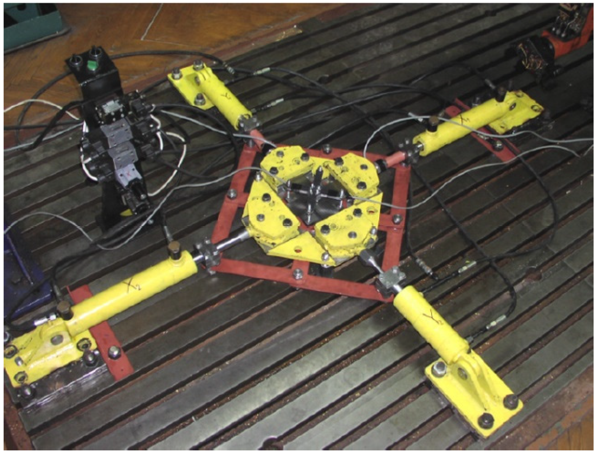
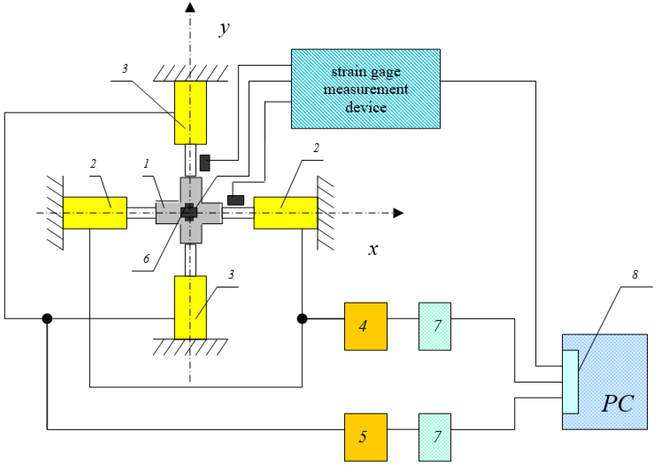
2.1. Technical Realization of the Hydraulic Loading Device

For the experimental evaluation of the elastic–plastic properties of sheet metals in plane stress using cruciform specimens, the device consists of:

• A hydraulic device for biaxial loading of the cruciform specimens;
• A dynamic strain gauge measurement device for sensing the evolution of the loading forces in the cruciform specimen arms using dynamometers with resistive strain gages;
• An extensometer for measuring the deformation in the central part of the cruciform specimen under biaxial tensile loading.
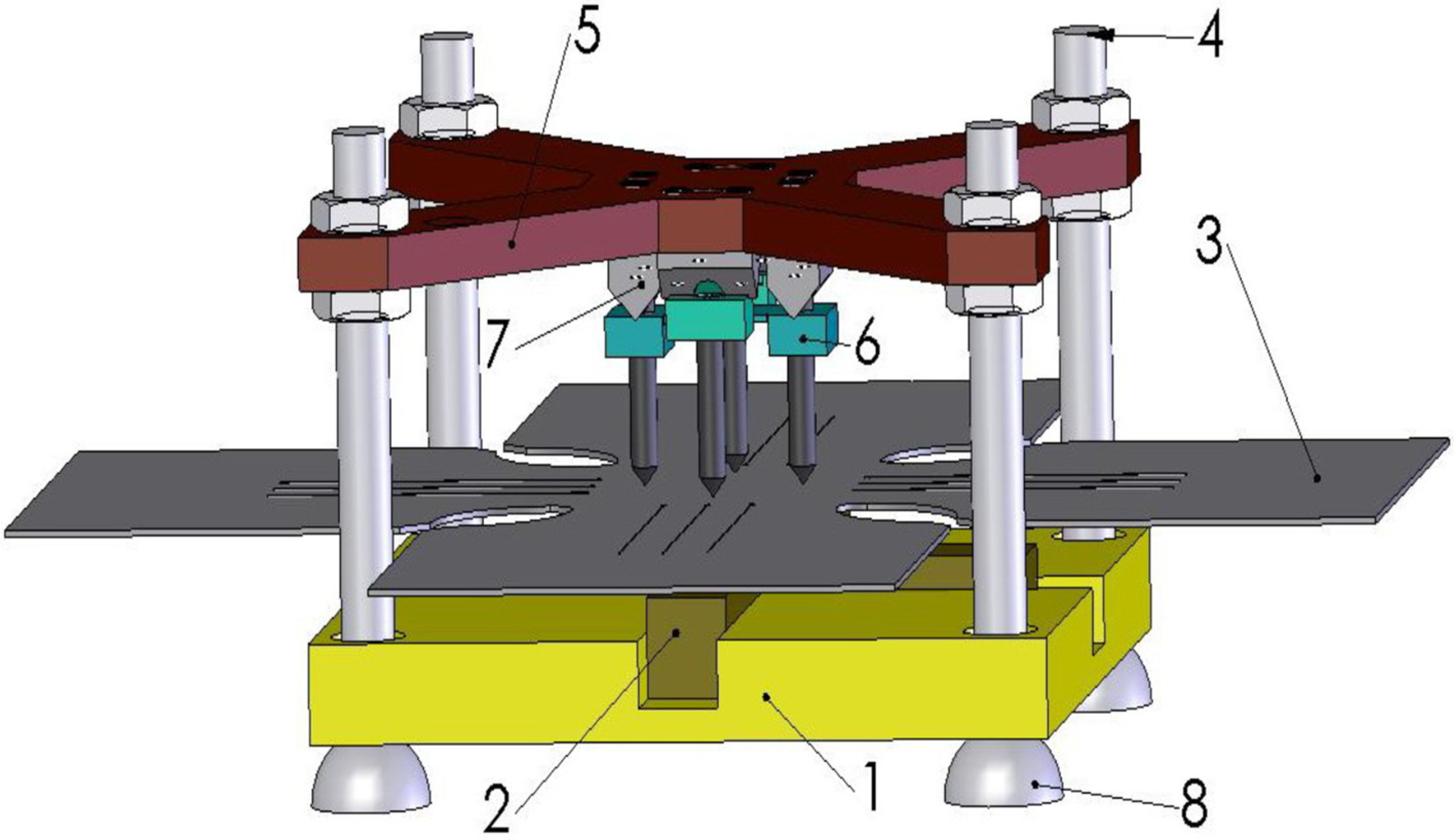
• The hydraulic loading device consists of the following main parts:
• A lamellar hydrogenerator SA33-100;
• Hydraulic cylinders;
• Clamping jaws;
• A guide body;
• Throttling valves;
• A main valve;
• Distributors of working fluid pressure;
• Electrical switches.

2.1.1. Lamellar Hydrogenerator SA3-100

A lamellar hydrogenerator is used for pressurized liquid sources. The working range of the hydrogenerator is from 0 MPa to 16 MPa. We set this range with the control valve VT2. An air cooler is installed to ensure the prescribed working fluid temperature.

The basic parameters of the device are:

• Power W = 7.5 kW;
• Maximum working fluid flow Q = 40 dm³·min⁻¹;
• Working temperature 50 °C;
• Maximum working pressure of 16 MPa.

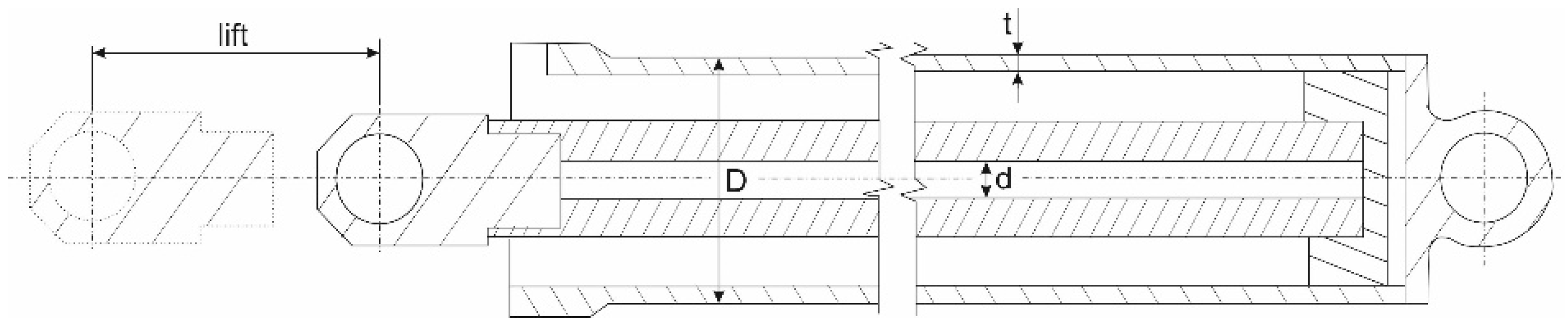
2.1.2. Hydraulic Cylinders and Hoses

By means of high-pressure hydraulic hoses, the pressure developed in the hydrogenerator enters the hydraulic cylinders. The rod, which is firmly attached to the hydraulic cylinder shown Figure 1, is attached to the dovetail grooves on the floor by means of a jig and screws. The jaws for clamping the cross pattern are attached to the movable rod.

The basic dimensions of the hydraulic cylinders are:

• Direction X: D = 63 mm, d = 32 mm, t = 6.5 mm, and lift= 250 mm;
• Direction Y: D = 60 mm, d = 32 mm, t = 6.5 mm, and lift= 100 mm.

2.1.3. Clamping Jaws and Guide Body

The clamping jaws are used to clamp the cross pattern. They move in the grooves of the guide body, which does not allow the jaws to deviate from the direction of loading. In this way, the additional load of the specimen, which is undesirable in this method of sheet metal testing, is eliminated. The guide body is fastened to the dovetail grooves on the floor with screws. When clamping the specimen, the upper and lower jaws are retracted. As the experiments occasionally released a specimen from the jaws, one steel roller was replaced by two grooved steel rollers located in a groove in the lower jaw, Figure 2. They cause deformation and pushing of the specimen into the groove in the upper jaw and thus secures the attachment of the specimen.

2.1.4. Parameters of the Main and Throttle Valves

The main valve controls the flow of the working fluid in the entire hydraulic circuit, Figure 3. The basic parameters are:

• Maximum working fluid flow: Q = 30 dm³·min⁻¹;
• Maximum working pressure: P= 35 MPa;
• Maximum working temperature: T = 80 °C.

Figure 3. The hydraulic scheme of the loading device, where: 1-Manually operated Needle Valve, 2-Manually Operated Check Valve, 3-Manually Operated Check Valve, 4-Solenoid Operated Modular Valve,4-Way, 2-Position Crossover Offset, 5-Solenoid Operated Modular Valve, 4-Way, 3-Position Tandem Center, 6-Solenoid Operated Modular Valve,4-Way, 3-Position Tandem Center.

Figure 3. The hydraulic scheme of the loading device, where: 1-Manually operated Needle Valve, 2-Manually Operated Check Valve, 3-Manually Operated Check Valve, 4-Solenoid Operated Modular Valve,4-Way, 2-Position Crossover Offset, 5-Solenoid Operated Modular Valve, 4-Way, 3-Position Tandem Center, 6-Solenoid Operated Modular Valve,4-Way, 3-Position Tandem Center.

The throttle valves are two-way throttle valves with stabilization. Using the first throttle valve, we control the speed of the jaws in the Y direction, and using the second throttle valve, we control in the X direction.

Throttle valve classification VSS2-206-1,6Q/JOO-1. The basic parameters are:

• Maximum working fluid flow: Q = 1.6 dm³·min⁻¹;
• Maximum working pressure: P= 32 MPa.

2.1.5. Electrical Switches

Switchboards are controlled by means of electrical switches. The main switch controls the two-position switchboard, which switches the pressure of the working fluid into the circuit to on or off. Switch X controls the load (thrust, pressure) in the x-axis direction, and switch Y controls the load (thrust, pressure) in the y-axis direction. The switches are supplied with DC voltage U = 12 V and current I = 5 A.

With the help of the high-pressure hydraulic pipes, the pressure developed in the hydrogenerator is transferred to the hydraulic cylinders. The rod, which is firmly attached to the hydraulic cylinder, is fixed to the grooves on the floor using a jig and screws. The jaws for clamping the cruciform specimen are attached to the movable rod.

A contact biaxial extensometer was used to measure the relative deformations in the central region of the specimen, shown in Figure 4. The extensometer consists of a fixed line (1) in which the movable slides (2) serve as a support for the sheet metal pressed by the spikes. The guide is mounted under the cruciform specimen (3), and the upper frame (5) for mounting the flexible members of the extensometer (6) is attached to it by four guide screws (4). The flexible members, together with the wedges (7) rigidly connected to the frame, form a pivoting fit by means of the rotatable fixing of the guide screws in the guide (8). The floating of the upper frame (5) of the extensometer is ensured in case of unwanted movement of the specimen as a rigid body during the test, Figure 5 [24,25,26].

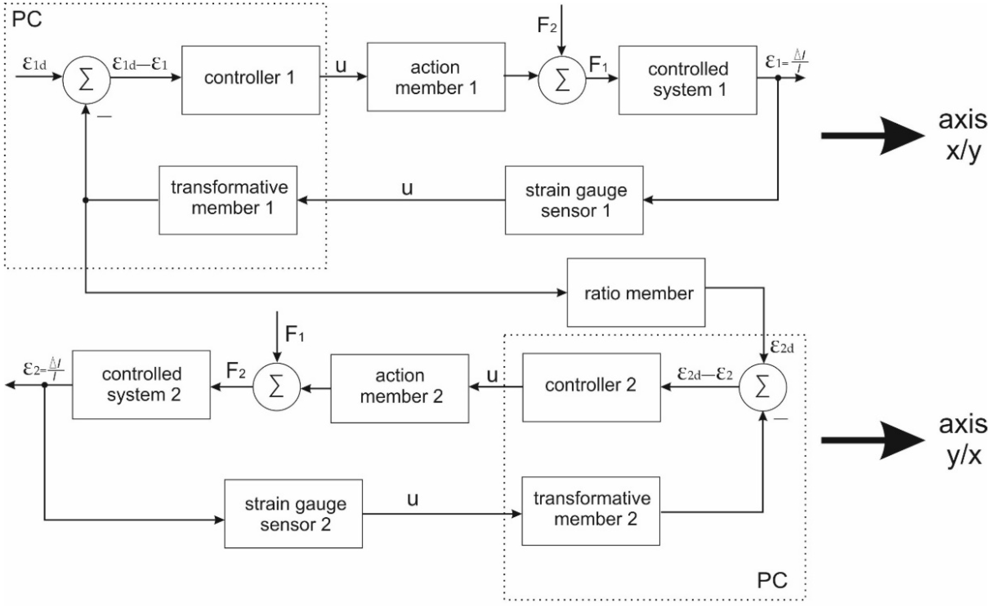
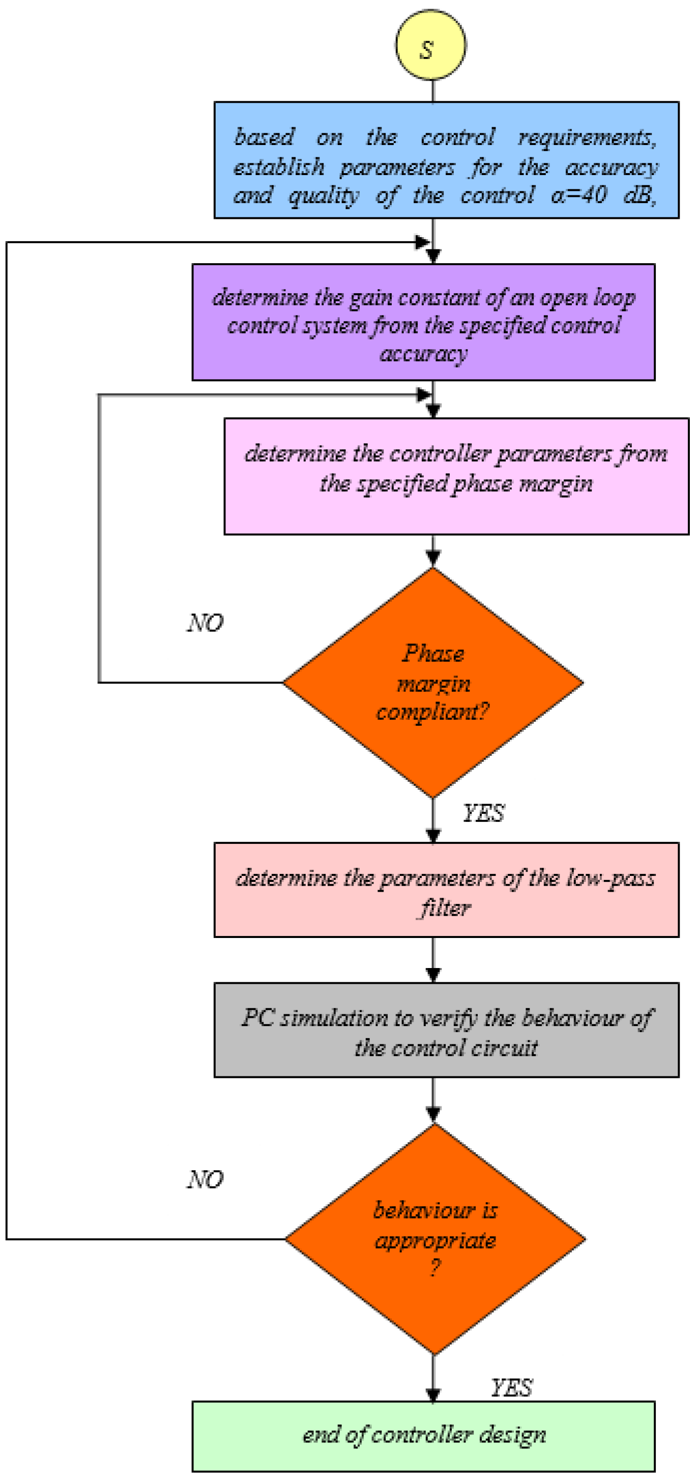
2.2. Load Mechanism Improvement through Regulator Design

The structure of the closed-loop control system in Figure 6 and Figure 7 consists of two autonomous one-dimensional closed-loop control circuits.

The role of these closed-loop control circuits is to ensure:

• Application of force to the testing specimen;
• Ratio regulation of deformations and mechanical stress;
• That the time change in the deformation will not be greater than prescribed in the relevant norm.

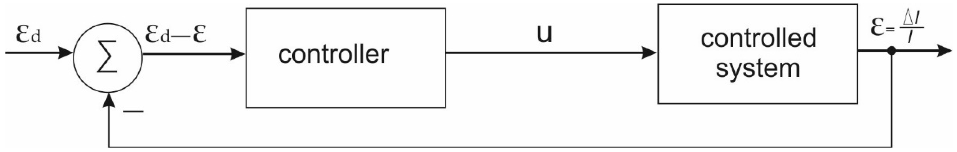
2.2.1. Regulator Design in a Block Diagram

The function of the first point (application of force to the testing specimen) is provided by both closed-loop control circuits. The function of the second point (ratio regulation of deformations and mechanical stress) is provided by closed-loop controller 2, and the function of the third point (that the time change in the deformation will not be greater than prescribed in the relevant norm.) is provided by closed-loop controller 1. In fact, these closed-loop controllers are not autonomous because each of the controlled variables varies depending on both action variables F1 and F2. The influence of the action variable of one closed-loop circuit on the other closed-loop control circuit, and vice versa, is taken into account here by means of error inputs. Regulator designs are presented in Figure 6. In the case of control circuit 2, both deformations, ${\epsilon }_1$ and ${\epsilon }_2$, and stresses, ${\sigma }_1$ and ${\sigma }_2$, are measured, respectively. The deformation, ${\epsilon }_1$, is multiplied by a dimensional constant in the ratio term, and after this adjustment, it is introduced as the desired value, ${\epsilon }_{2d}$, into the control circuit 2, respectively, and introduced as the desired value, ${\sigma }_{2d}$. Function 3 is provided by the control circuit 1 by feeding the desired value input with such a waveform of the desired deformation value such that the temporal variation of the desired values of ${\epsilon }_{1d}$ and ${\sigma }_{1d}$, respectively, during the entire testing process are not greater than those required by the standard.

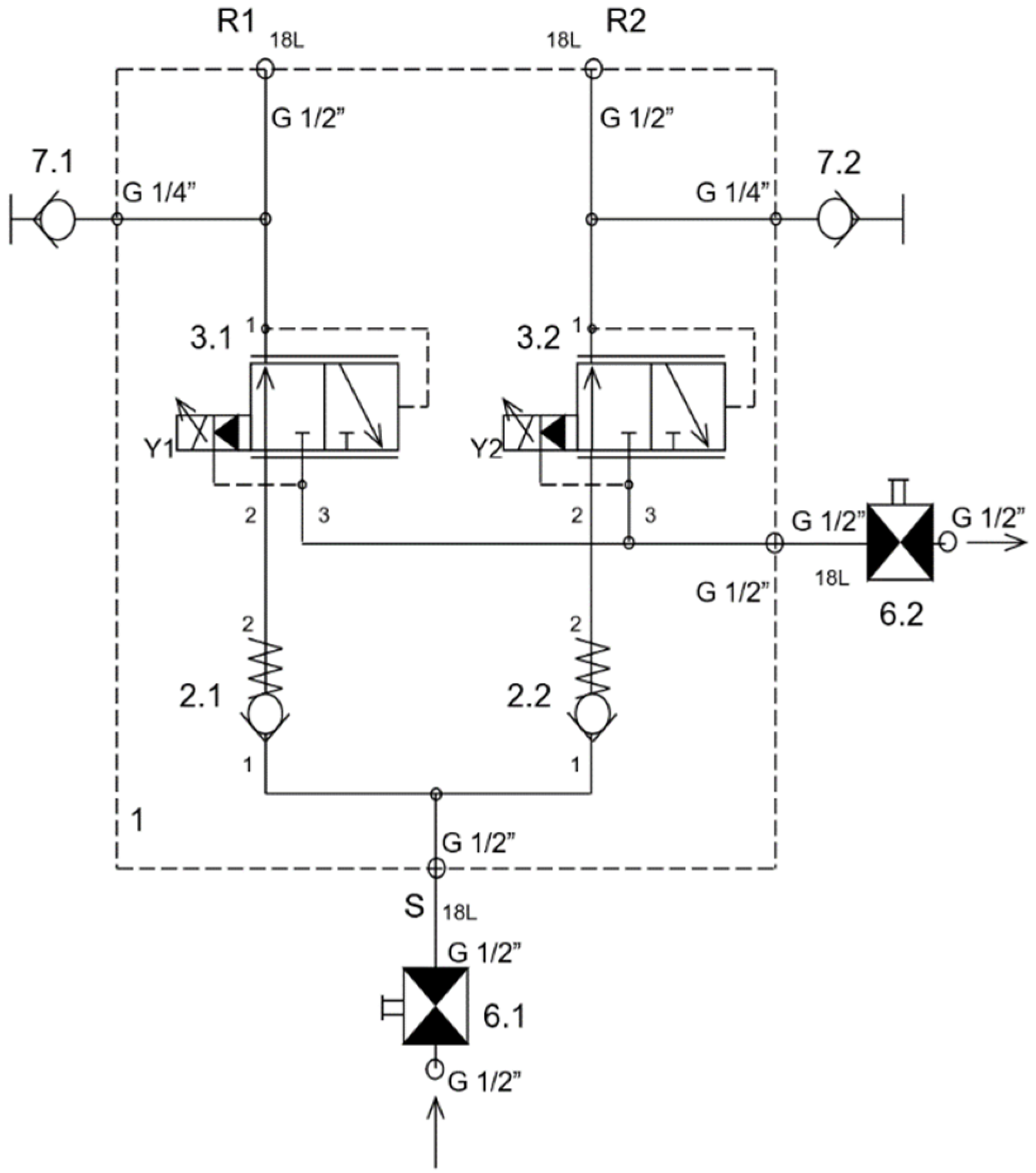
2.2.2. Modernization of the Hydraulic Control Circuit

In order to apply the automated approach, it was necessary to replace the manually operated pressure-reducing valves with the PDR08P-01 pressure-reducing valves, which can be controlled by an electrical signal. The modernized control unit is used to reduce the pressure of the hydraulic fluid at the outputs of the control unit, R1 and R2, to the hydraulic cylinders of the loading device. Hydraulic fluid is supplied to the control unit via inlet S. Constant regulated pressure exits from outlets R1 and R2. Waste from outlet T must be led to the tank. The proportional pressure-reducing valve 3.1 (3.2) maintains a constant pressure at the outlet R1 (R2), Figure 8.

A computer equipped with a multifunction card MF-624 is used as a controller. This card, or similar, is necessary for the purpose of connecting the computer to the real environment. It contains an 8-channel 14-bit AD converter with simultaneous sampling, 8 independent 14-bit DA converters, 8-bit digital inputs, 8-bit digital outputs, and 4 inputs for incremental position sensors. The card is operated by the Real-Time Toolbox in the MATLAB/Simulink program. Since the MF 624 multifunction card (MF 604) does not have a current output, an RB-01-TU-002-100-E voltage–current converter has been designed. The computer output of 0–10 V is applied to clamp number 3 and 4 for x-axis control and to clamp number 10 and 11 for y-axis control. At clamp number 5, 6, 7, 12, 13, and 14, respectively, a potentiometer is connected, which allows for the manual control of the output current. Clamps 1 and 2 control the valve on the x-axis, and 8 and 9 control the y-axis. Both of these converters are powered by a stabilized source GU1, which is connected to the main voltage.

The analog inputs AD0 and AD1 of the MF624 multifunction card are fed with signals from the strain gauge apparatus, which are processed and evaluated by the MATLAB/Simulink simulation program according to the specified input requirements. Subsequently, the analog outputs DA0 and DA1 control the electronics of the actuators of the PDR08P-01 valves, Figure 9.

3. Mathematical Model

The aim of this section is to compile the mathematical models of the individual elements of the control circuit. When compiling mathematical models, individual functional subsystems were systematically defined. An important level of correct system-wide description was to define the physical principle with a subsequent mathematical description. The mathematical model was created in the MATLAB/Simulink environment and the Laplace transform was used to describe the resulting transfer function.

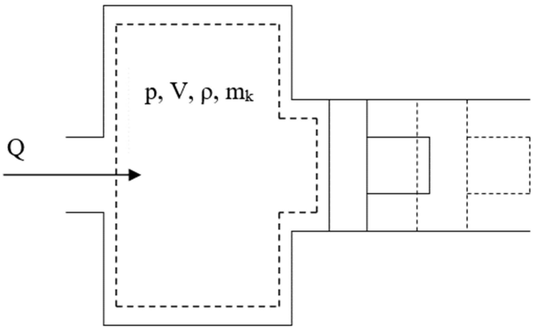
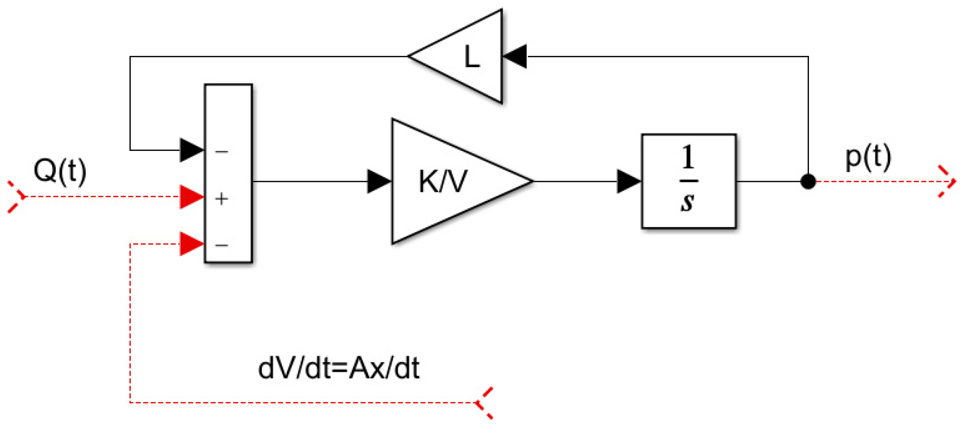
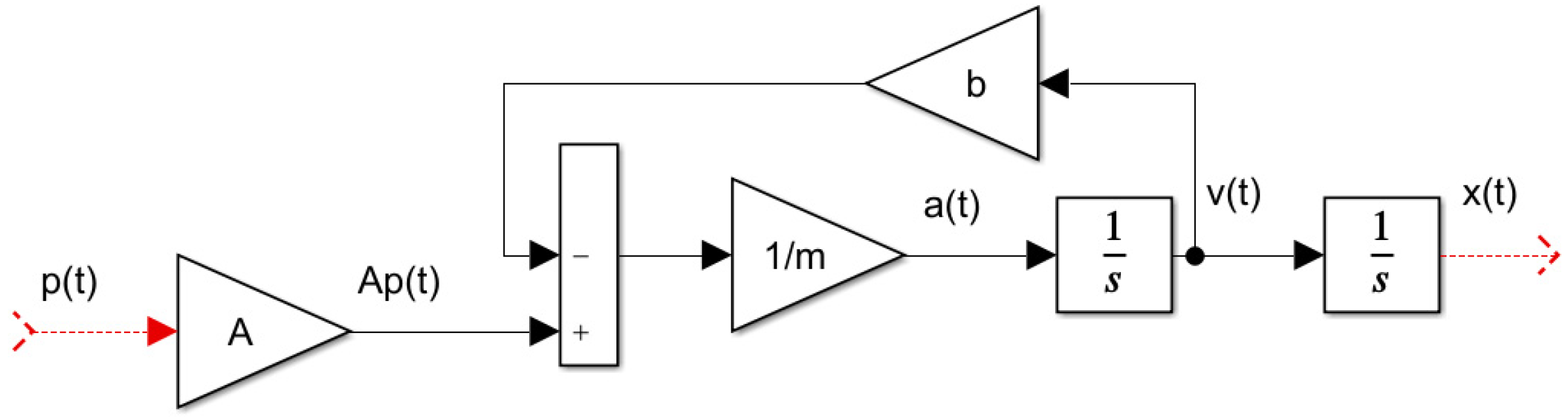
3.1. Mathematical Model of the Electrohydraulic Actuator

The engine hydraulic subsystem is described by the formula between the pressure in the cylinder chamber and the oil volume flow into the linear hydraulic motor. From a control point of view, this is an important relationship because the compressibility of the oil creates a “spring” effect in the cylinder chamber of the hydraulic motor, which interacts with the weight of the piston, resulting in resonance in the low-frequency range. This effect is present in all hydraulic systems and, in many cases, unexpectedly limits the usable bandwidth.

In Figure 10, the cylinder chamber is filled with pressurized hydrostatic oil; the pressure and density in this volume are the same at all points in the chamber. The instantaneous mass of the pressure fluid in the volume of the cylinder is given by the following equation:

$$m_k=\rho V,$$

(1)

where ρ—density of the liquid and V—volume of the liquid in the cylinder. By differentiating Equation (1) according to time, we obtain the time change in mass expressed as:

$$\frac{d{m}_k}{dt}=\frac{d\rho }{dt}V+\rho \frac{dV}{dt},$$

(2)

From the law of conservation of mass, it is possible to write the left side of Equation (2):

$$\frac{d{m}_k}{dt}=\rho Q,$$

(3)

where Q is the total liquid volume flow. It follows from the equation of state of liquids that:

$$\frac{d\rho }{dt}=\frac{\rho }{K}\frac{dp}{dt},$$

(4)

where K—volume modulus of elasticity. Substituting Equations (3) and (4) into Equation (2) with subsequent adjustments, we obtain the relation:

$$\frac{dp\left(t\right)}{dt}=\frac{K}{V}(Q\left(t\right)-\frac{dV}{dt}-Lp\left(t\right)),$$

(5)

where L characterizes the oil flow between the piston and the cylinder wall, and Equation (5) represents a mathematical model of the hydraulic subsystem of the hydraulic motor.

In block expression, this model is shown in Figure 11.

The mechanical subsystem of the hydraulic motor describes the movement of the piston of the hydraulic motor due to the applied hydrostatic pressure of the oil. This equation can be expressed by Equation (6):

$$m\frac{d^{2}x(t)}{d{t}^2}+b\frac{dx(t)}{dt}=Ap(t),$$

(6)

where m is weight of the piston, x is load path, and b is viscous damping. In block expression, this equation is shown in Figure 12.

3.2. Mathematical Model of the Proportional Pressure-Reducing Valve

Hydraulic control valves are used in the hydraulic circuits for precise regulation and control of the entire hydraulic system. When controlling the hydraulic circuit, the valve provides a connection between the sensor, the pump, and the hydraulic output device. This valve is a member which, by means of feedback from the operator or another automatic control source, sets the system output (i.e., pressure or flow) adequately. It is this feedback that provides a controllable output for the hydraulic system and provides a safe function that is essential when working with high-performance equipment, which is a typical hydraulic application, Equation (7), Figure 13.

$$Q=k_{i}i-k_{p}p,$$

(7)

where k_i is the sensitivity and k_p is the compliance of the valve, Equation (8).

$$k_i=\frac{dQ}{di}\stackrel{•}{=}\frac{\Delta Q}{\Delta i}, k_p=\frac{dQ}{dp}\stackrel{•}{=}\frac{\Delta Q}{\Delta p},$$

(8)

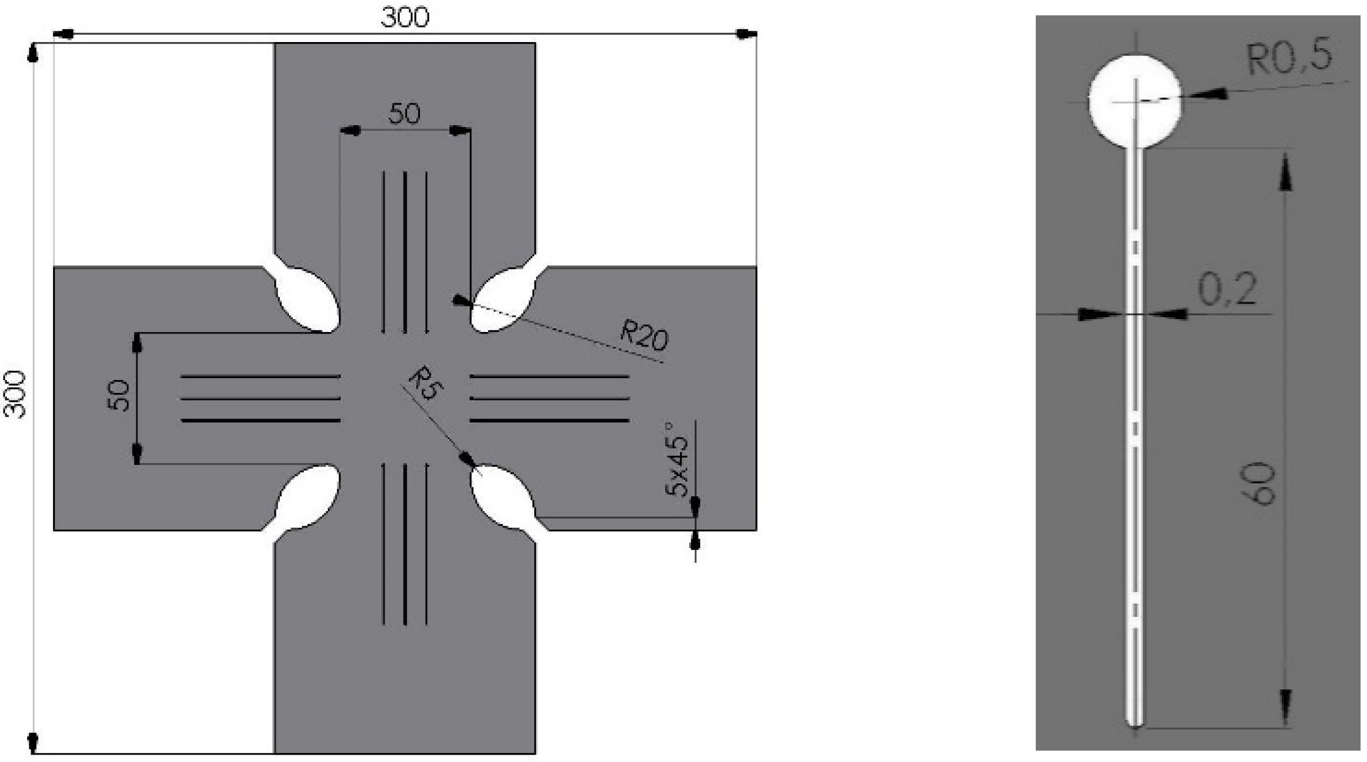
3.3. Mathematical Model of the Cruciform Specimen

The mathematical model of the cruciform specimen is based on a real model of the specimen. The real model of the specimen was prepared according to the drawing documentation, where the basic dimensional parameters were given.

Each part of the cruciform specimen has notches burned by a laser, Figure 14, to eliminate bending and shear loads in the central part of the specimen. For the purposes of controller design, we have proposed the following mathematical (simplified-linear in elastic regions) model of the metal cruciform specimen, Equation (9):

$$F=k_z\Delta l$$

(9)

Part of the verification of the cruciform specimen is using a numerical approach for the application of the finite element method. The cruciform specimen ratio $F_x:F_Y=1$ will be considered in the FEM simulation. The distribution of stresses, ${\sigma }_x$ and ${\sigma }_x$, and plastic strains, ${\epsilon }_x^P$ and ${\epsilon }_y^P$, in the middle part of specimen was determined by the coefficients $k_x, k_y,g_x, \mathrm{and} g_y$ according to Equations (10)–(12)

$$k_x=\frac{{\sigma }_x}{{\sigma }_{x0}}, k_y=\frac{{\sigma }_y}{{\sigma }_{y0}}$$

(10)

$${\sigma }_{x0}=\frac{F_x}{b·t}, {\sigma }_{y0}=\frac{F_y}{b·t}$$

(11)

$$g_x=\frac{{\epsilon }_x^P}{{\epsilon }_{sx}^P}, g_y=\frac{{\epsilon }_y^P}{{\epsilon }_{sy}^P}$$

(12)

where $b$ is the width of the arm of the cruciform specimen, $t$. is the thickness of the cruciform specimen, and ${\epsilon }_{sx}^P$ and ${\epsilon }_{sy}^P$ are plastic strains in the middle of the cruciform.

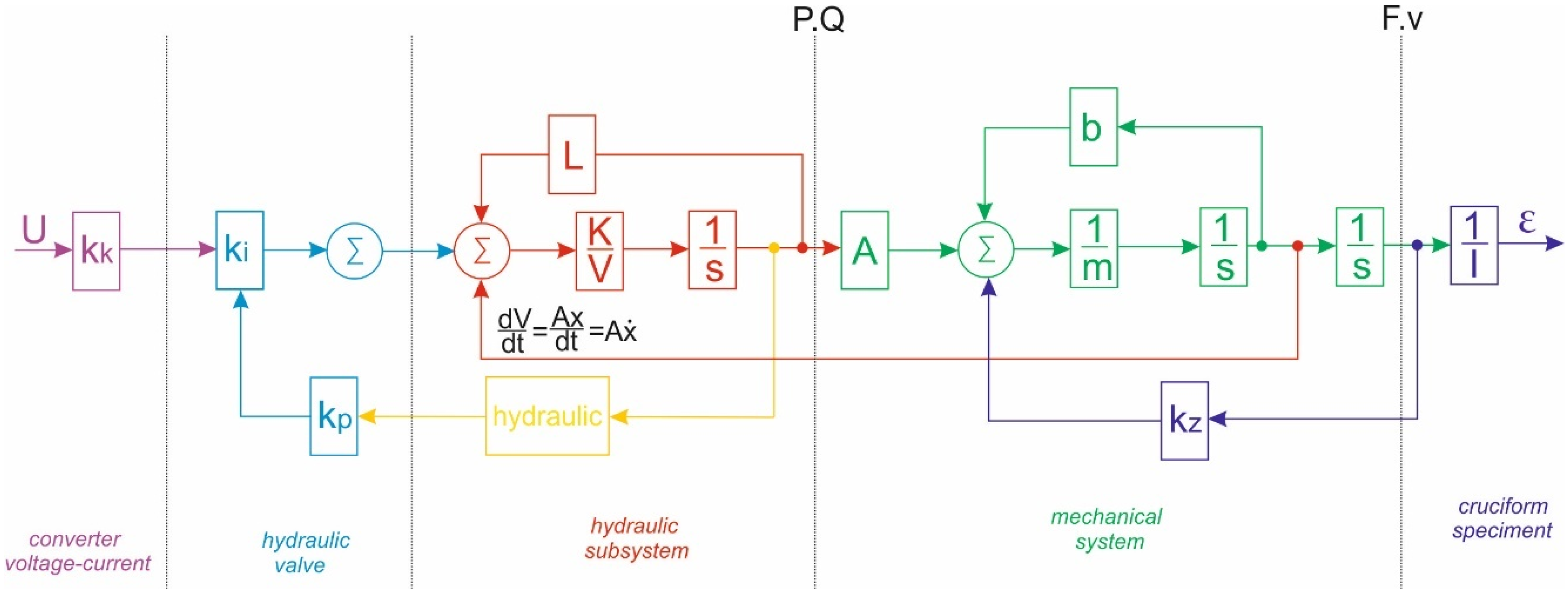
3.4. Design of the Resulting Block Diagram of the Control Circuit

The resulting closed-loop block diagram, Figure 15, is composed of individual parts of blocks or nodes depending on the type of mechanical, hydraulic, and test functionality.

After mathematical modifications and reductions using block algebra methods, we obtained the final form of the image transmission of the entire system:

$$\frac{\Delta l(s)}{U(s)}=\frac{k_{i}KA{k}_k}{\{mV{s}^3+(Km{k}_p)s^2+[k_{z}V+K{A}^2]s+K{k}_z{k}_p\}}$$

(13)

When designing the controller, we used the derived models of the individual elements of the closed-loop control circuit, Figure 16.

We designed the controller in the frequency domain, using the method of shaping the frequency response of an open control circuit. In this method, the frequency response is shaped according to the requirements of the control circuit, namely in the low-frequency range, the mid-frequency range, and the high-frequency range. The frequency response in the low-frequency range is designed according to the control accuracy requirements. The frequency range of this range is determined based on the setpoint and fault signal power distribution. In our case, we consider the desired value. In order to determine the frequency range in the low-frequency range, we needed to know the time course of the setpoint. We assumed that the time change will take place at a constant rate, Figure 17. The central frequency determines the quality of the regulation that will characterize the phase margin. The literature recommends the value of the phase margin, φ_m, to be in the range of 30° to 60°. In our case, we choose the value in Equation (14).

$${\phi }_m=45°$$

(14)

In order to have a stable control loop, the frequency–amplitude directive combustibility characteristics must be below −40 dB/decade. The area of high frequencies no longer has a significant effect on the quality of regulation, but it has an effect on the amount of noise, which in most cases is concentrated in this area. However, the noise characteristics are unknown to us at this design level, but we will nevertheless design a low-pass filter of the 2nd order in the high-frequency range. The final algorithm of the controller design is shown in Figure 18.

4. Results

4.1. Design of the Resulting Block Diagram of the Control Circuit

It is clear from the transfer function of the S(s) system that this transfer function is static, so if we want to reach the final value of the control accuracy, the transfer function of the open control circuit R(s)S(s) must be of type 1 (because at the setpoint input, the signal changes at a constant rate). It follows that for the open control loop R(p)S(s) to have completed the required control accuracy for the type of the input signal, it is necessary that the controller contains an integration component, wherein the transfer function is Equation (15) and the Bode characteristic of the system S(s) is shown in Figure 19.

$$R_i\left(s\right)=\frac{r_i}{s}$$

(15)

After the implementation of the integrating components, we can see in Figure 20 that the closed-loop control is unstable and is safeguarding the required quality control as a member with phase advance, Equations (16) and (17), Figure 21:

$$R_f=\frac{\sqrt{\alpha }s+{\omega }_c}{s+\sqrt{\alpha }{\omega }_c},$$

(16)

were,

$$\alpha =\frac{1+\sin \left({\mathrm{\Phi }}_{\max }\right)}{1-\sin \left({\mathrm{\Phi }}_{\max }\right)}$$

(17)

The controller includes a low-pass filter of the 2nd order with transmission, which allows the suppression of signal noise in the high-frequency range, Equation (18) and Figure 22.

$$Rd=\frac{{\omega }_d}{s^2+2\zeta {\omega }_d+{\omega }_d^2},$$

(18)

For the correct functionality of the overall designed control system, a simulation of the control circuit (closed loop) for deformation control was performed, providing that if the required value of deformation changed at a constant speed, it would be applied to the input, Figure 23.

The aim of this simulation was to verify the behavior of the controlled variable on the input signal. In addition, it is also important to determine whether the output variable from the controller is saturated, Figure 24. Based on the computer simulation performed, it can be concluded that the designed controller meets the requirements imposed on the control circuit.

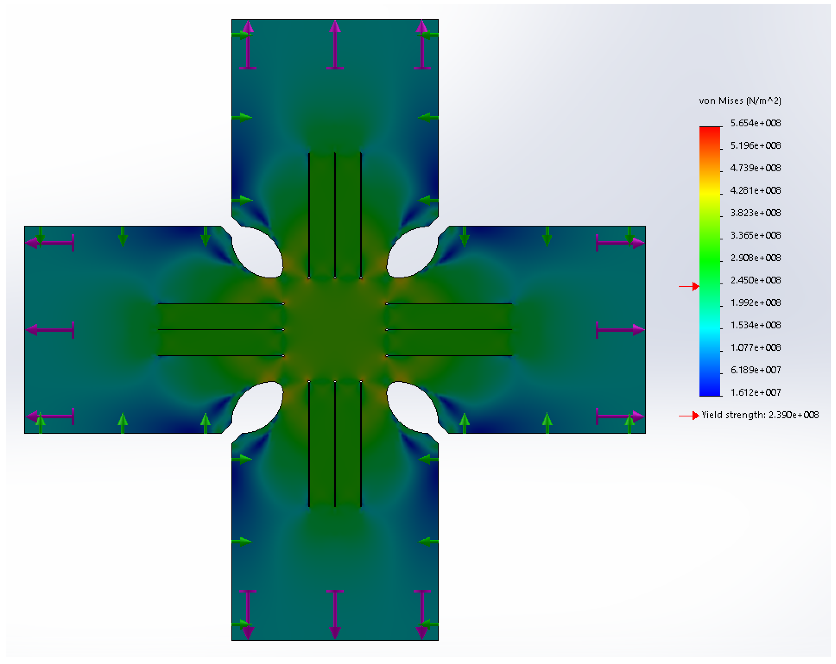
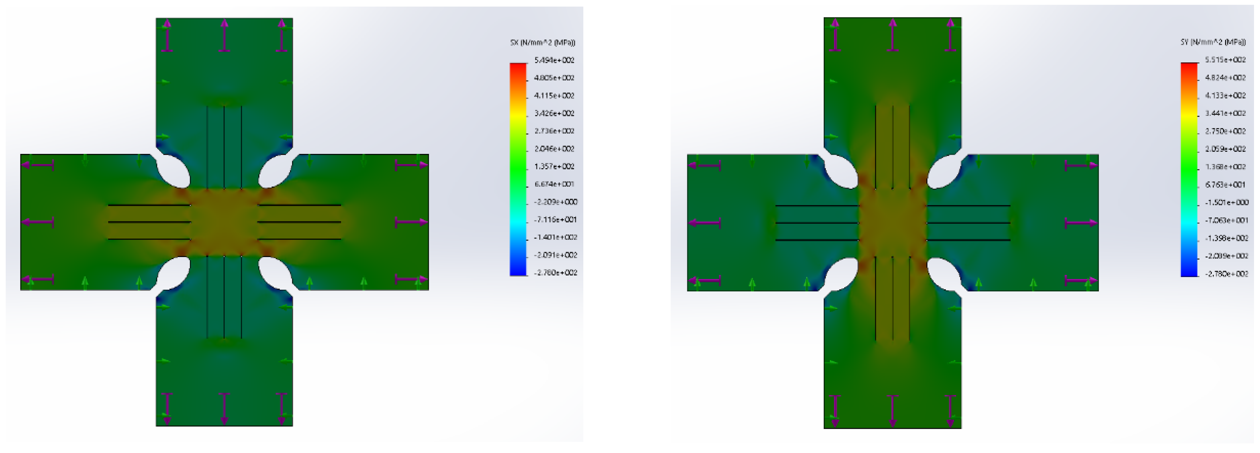
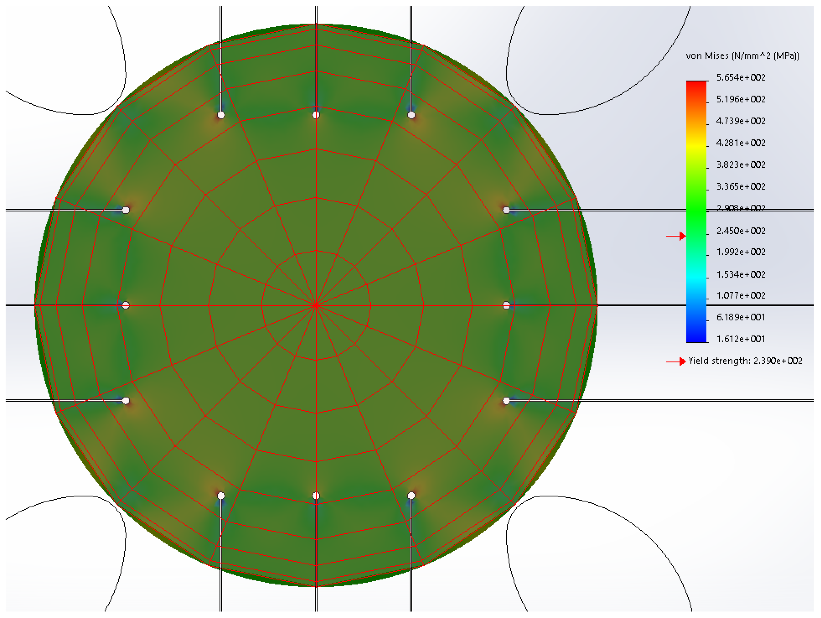
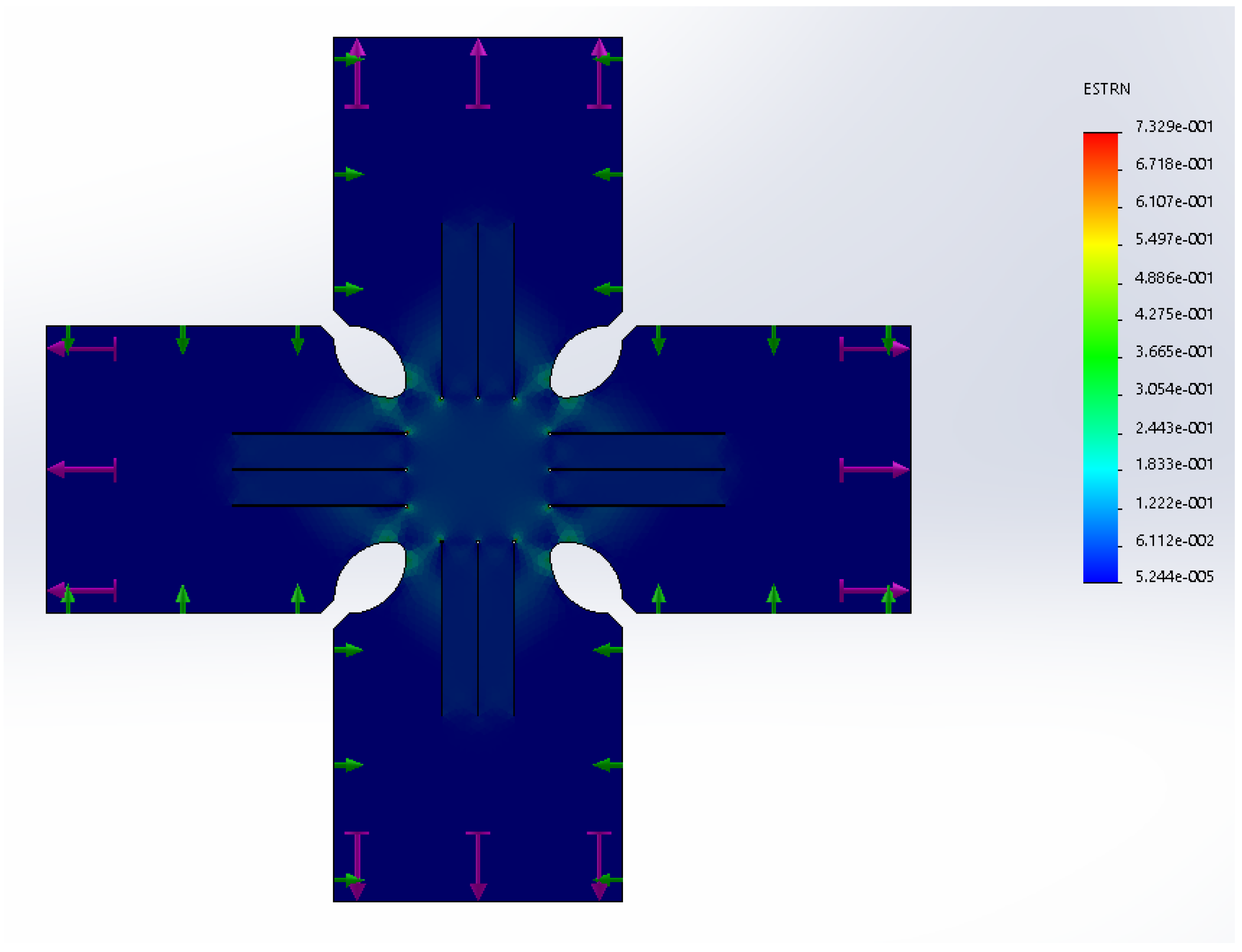
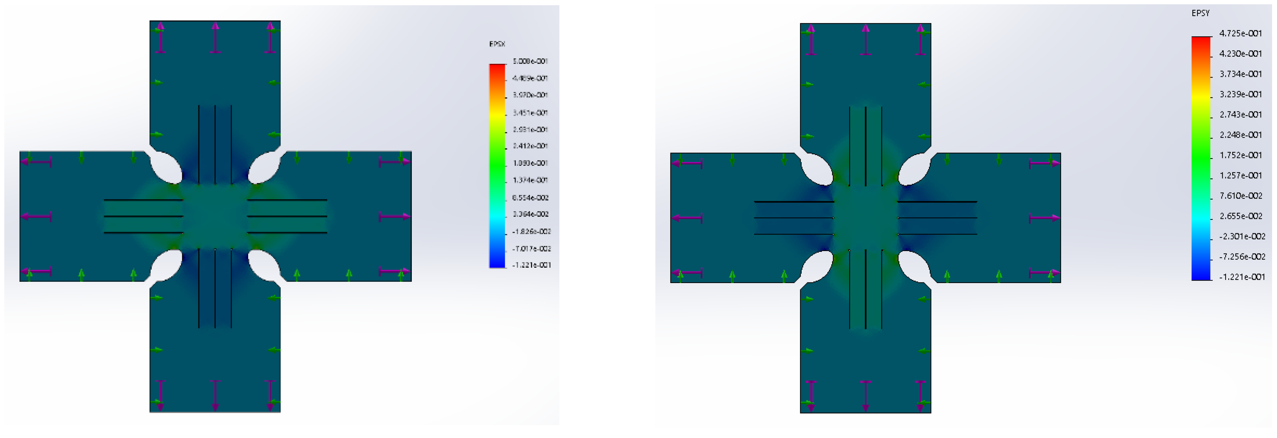
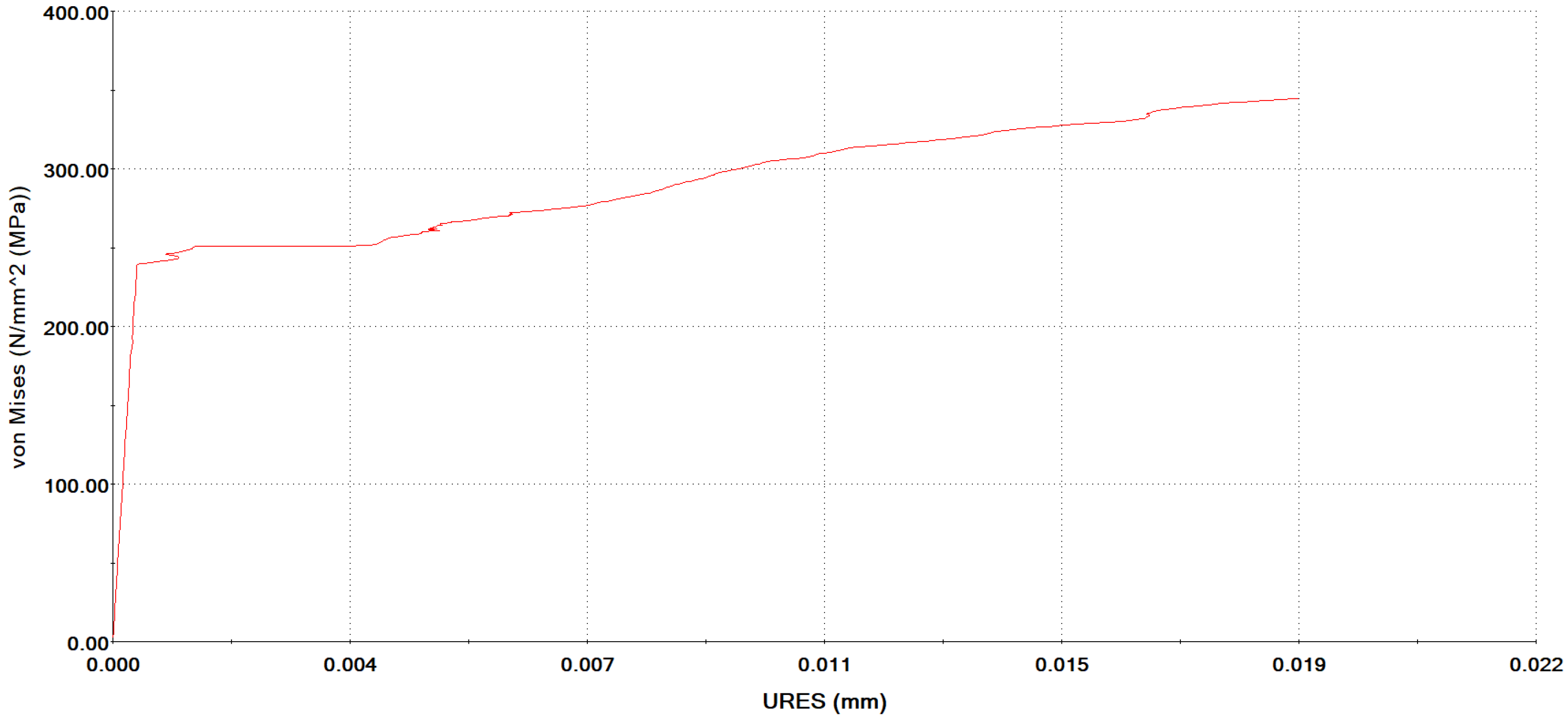
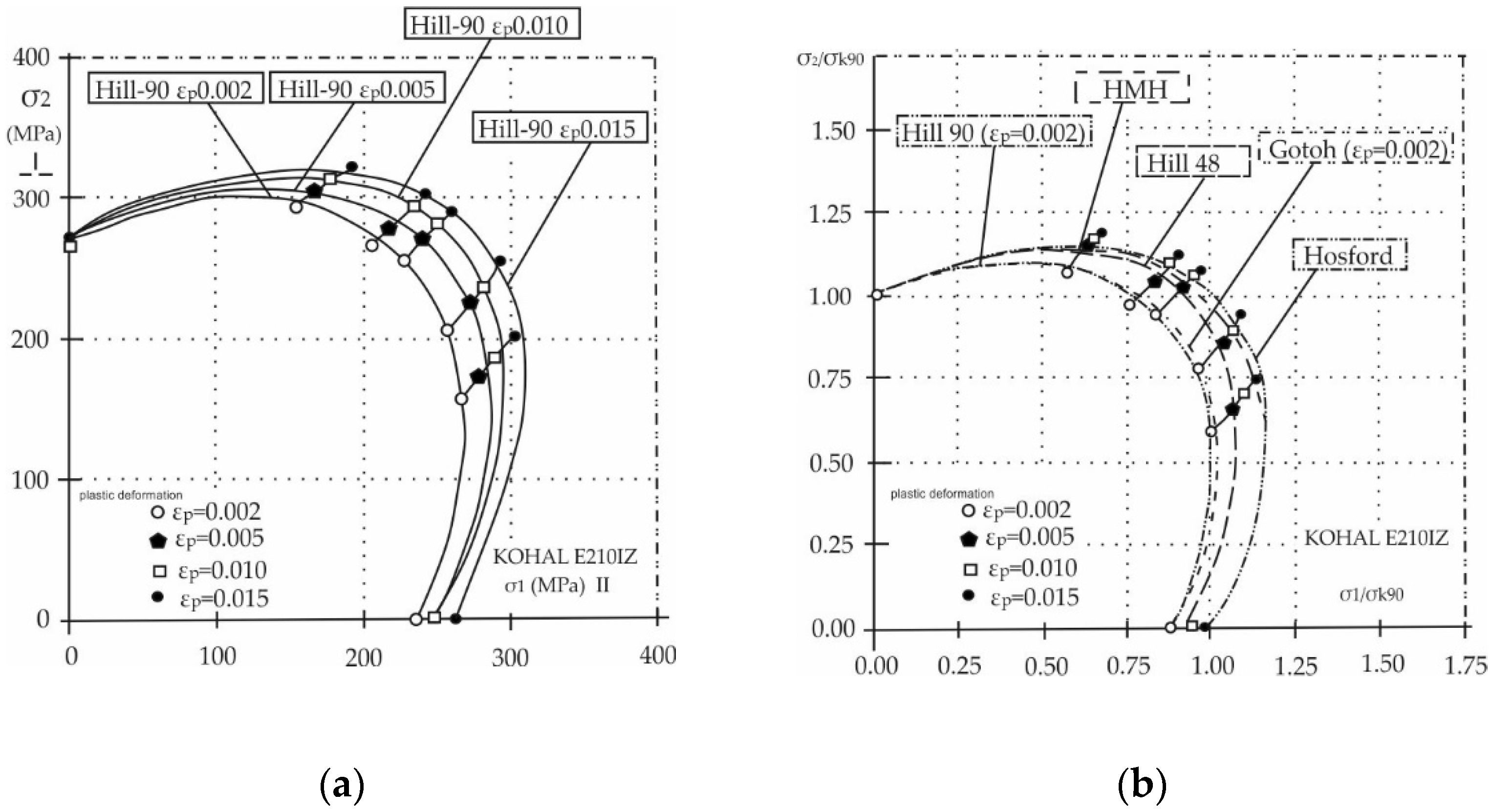
4.2. Nonlinear FEM Simulation of the Specimen Based on the Plasticity Anisotropic Material Model

The numerical simulation’s task is to simulate and verify the deformation behavior of the cruciform specimen clamped in the loading device. In order to verify the deformation behavior of the cruciform specimen, we had to create a numerical model of the specimen with specific geometric parameters. Since, in this case, it is a gradual loading of the sample, the total simulation time was set at 60 s, similar to the case of experimental verification. During preprocessing, the simulation parameters were set so that the course of the simulation corresponded as closely as possible to the real experimental verification. The simulation was performed through the simulation module within the Solid-Works 2017 software. First, the solved problem was chosen as nonlinear static. Subsequently, the boundary conditions of the simulation were defined as acting forces, connections, and material characteristics. Since, within the experiment, we used the material Kohal E 210 IZ, whose numerical model was defined as nonlinear plastic von Mises, and at the same time, the deformation criterion according to Max von Mises stress was chosen, the material specifics were defined by means of the specified stress–strain curve of Kohal E210 IZ. The blended curvature-based mesh principle was used for the meshing process. The entire mesh consisted of 16,738 elements and 34,781 nodes with 103,759 degrees of freedom. The resulting mesh parameters were set based on the following findings:

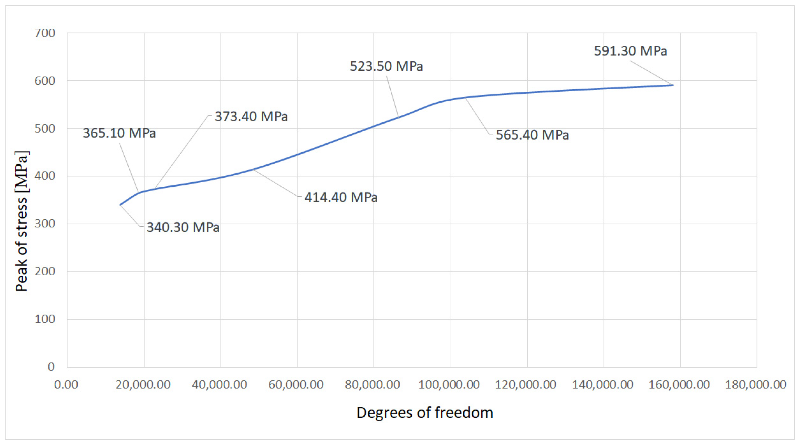
• Several mesh configurations were checked, and the dependence of the change in the peak stress on the change in degrees of freedom was realized, together with the dependence of the peak stress on the change in the number of elements. In this way, the convergence of the mesh was verified, Figure 25;
• The upper limit of the maximum stress was set at which the calculation was still stable without the need for drastic changes in the convergence tolerance and singularity elimination factor;
• The minimum element size was determined based on geometric parameters at 0.078 mm, and the maximum element size was determined based on convergence properties at 2.62 mm.

The software automatically selected the Large Problem Direct Sparse solver core, which is used for problems with large displacements, to solve the problem. The course of the simulation can be evaluated in mainly two important phases, including a linear increase in stress without significant visible displacements and a nonlinear change in stress with a nonlinear change in displacements from the point exceeding the yield point of the material. It is in this situation that plastic deformations occur on the sample, which is important for us due to the nature of the task in order to identify the overall change and the course of stress and strain during axisymmetric loading.

The obtained results from the postprocessing phase of the FEM simulation are presented in the following figures: Figure 26, Figure 27, Figure 28, Figure 29, Figure 30, Figure 31, Figure 32, Figure 33, Figure 34 and Figure 35. These results can be divided into two basic groups. The first group contains a graphic representation of stress and strain at the end of the simulation at the time of 60 s, Figure 26, Figure 27, Figure 28, Figure 29, Figure 30 and Figure 31. The second group of images shows the characteristics of the change in values, the dependence of the identified center of the cruciform specimen, and the corresponding node within the mesh of finite elements.

In Figure 26, the stress curve of the cruciform specimen according to von Mises is shown. The yield strength value is clearly identified in the legend. It is clear from the picture that the stress under axisymmetric loading has a symmetrical character, while its greatest intensity is found in the faintly yellow areas and areas around the sections that were added to eliminate bending and shear loads on the specimen. The largest numerically identified stress is found in the areas around the holes and longitudinal cuts. In Figure 27, the iso clipping display method is applied to delimit the area from the specified stress value. As part of the postprocessing phase, we set the yield strength as a limit value in order to clearly identify the area where the stress is greater than the value of the yield strength and where plastic deformations occur. The resulting region clearly supports the assumption of the location of the extensometer apparatus as in Figure 4. In Figure 28, we can observe a pair of von Mises stress distribution images in the direction of the x-axis and in the direction of the y-axis, which actually allows us to obtain the stress, ${\sigma }_x$, at a specific point in the direction of the x-axis and the stress, ${\sigma }_y$, in the direction of the y-axis. In more detail, the stress and its dispersion can be observed on the central section in the middle of the selected area, Figure 29. It is clear from the characteristics of the image, that the entire area is affected by plastic deformation.

In the center of the section, there is an elementary element with the corresponding nodal points. In the areas where the yellow coloring occurs, until it turns red, the stress is concentrated, and according to the values, the tensile strength can be reached. These areas primarily occur around the holes and cuts, which, as already mentioned, are applied purposefully with the aim of reducing shear and bending stress components. We can see the strain of the cruciform specimen at the seventieth second of the simulation in Figure 30. Similar to the stress and strain, we can see the symmetrical character of their dispersion. Analogously, the largest values occur in the area of holes and longitudinal sections, thus, to a certain extent, copying the area of the stress concentrations. Figure 31 shows the results of the simulation of the proportional extension ${\epsilon }_x$ in the direction of the x-axis and ${\epsilon }_y$ in the direction of the y-axis. From the graphic representation of the strain dispersion, we can conclude that the central investigated area has smaller values than the areas in green around the longitudinal sections and holes. In the next part of the analysis, we focused on evaluating the results from the entire duration of the simulation, which is sixty seconds, for a specific node of the FEM mesh with the number 34,331. This node is characterized by the fact that it is geometrically closest to the symmetrical center of the part. Since this is a nonlinear task, the individual time periods of the simulation were processed approximately according to the set criteria of the solver. The total number of simulation steps thus consisted of 463 partial results. These partial results, depending on the selected characteristic, are presented on the graphs in Figure 32, Figure 33, Figure 34 and Figure 35. In Figure 32, the dependence of the stress in the investigated node on the simulation time can be seen.

After exceeding the yield strength, the stress in the plastic region continues to rise, but the rise is no longer as purely linear as in the case of the elastic region. Another picture, Figure 33, presents the dependence of the displacements on the simulation time. Analogously, at the time of the 40th second, which is again represented by exceeding the yield strength, a dramatic change occurs. This consists of a high increase in displacement in the plastic area. Structurally, significant plastic deformations occur in the material, which is manifested by the just-mentioned displacements of the investigated node.

Figure 34 shows the graph of the dependence of stress ${\sigma }_x$ in the direction of the x-axis and ${\sigma }_y$ in the direction of the y-axis, where ${\sigma }_y={\sigma }_y\left({\sigma }_x\right)$. The mentioned characteristic has a linear character, while the obtained values of ${\sigma }_x$ and ${\sigma }_y$ are almost identical, which corresponds to the simulation requirement for the load ratio of the sample $F_1:F_2=1$. Another graph, obtained from the postprocessing phase, is shown in Figure 35. It shows the characteristics of the change according to von Mises within the deformation displacement in the mentioned node. You can clearly see a significant increase in stress up to the moment of crossing the yield strength limit, when the deformation displacements started to grow bigger and bigger. Thus, plastic changes occur in the form of displacement of part of the sample. It is necessary to note that while the mentioned node was investigated in the analysis, the situation in the other nodes of the mesh is different. For example, in the peripheral regions of the sample, which are held in the jaws, there are displacements in the order of millimeters, while the displacements in the central region are in the order of hundredths to tenths of a millimeter. For illustration, we selected several values of strain at specific steps of the simulation within the plastic deformation,

Table 1. Table of numerically computed values of strain in some selected steps.

Selected Step of Simulation	Computed Value—Strain in Plastic Deformation (Center of Specimen)
In 100	${\epsilon }_x^s=0.001945$$, {\epsilon }_y^s=0.001944$
In 150	${\epsilon }_x^s=0.008585$$, {\epsilon }_y^s=0.008582$
In 200	${\epsilon }_x^s=0.01153$$, {\epsilon }_y^s=0.01152$
In 250	${\epsilon }_x^s=0.01615$$, {\epsilon }_y^s=0.01614$
In 463 (final)	${\epsilon }_x^s=0.03418$$, {\epsilon }_y^s=0.03415$

.

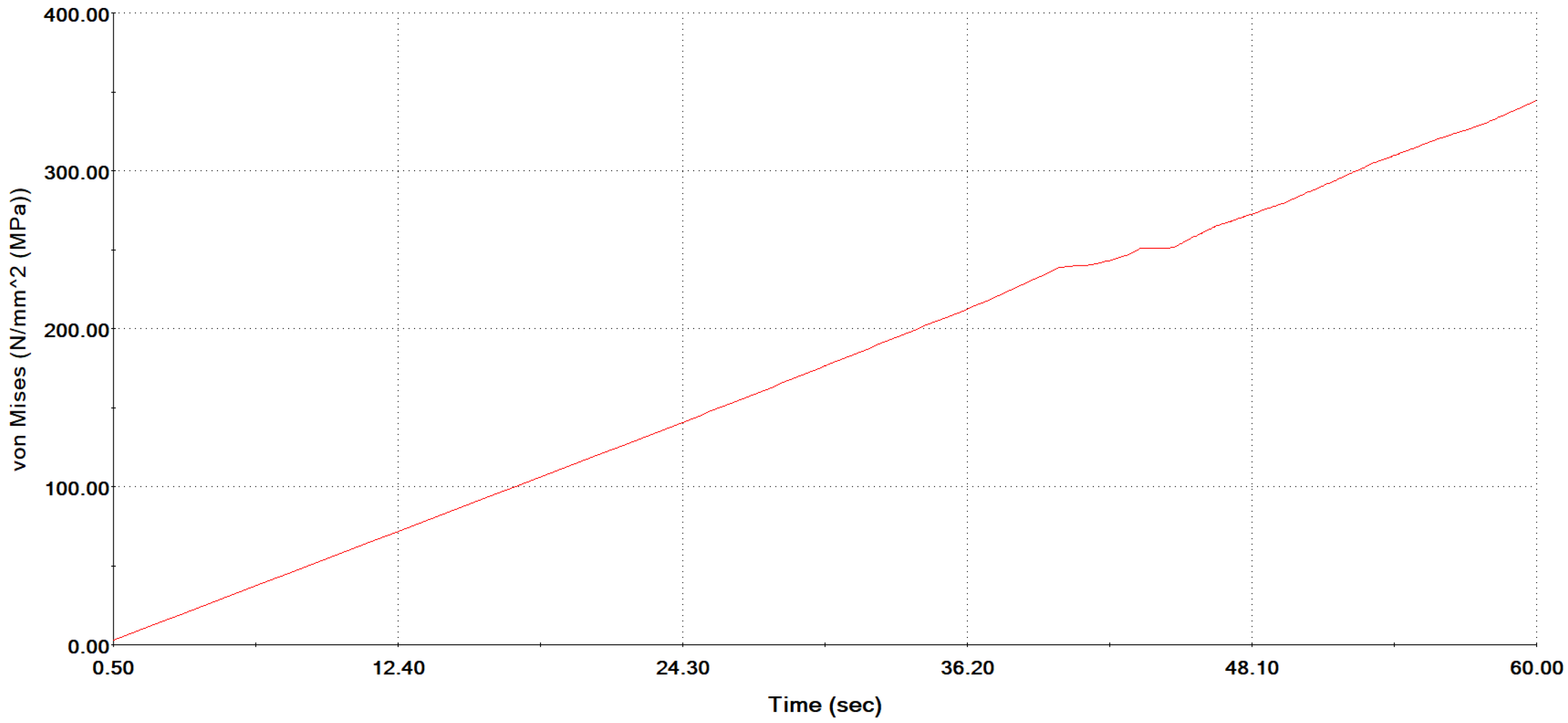
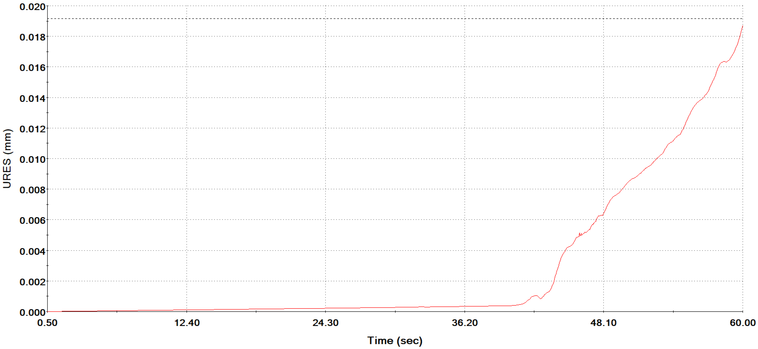
4.3. Experimental Verification of the Closed-Loop Control System and the Plasticity Properties of the Cruciform Specimen

The content of this subsection is the experimental verification of the closed-loop control system mentioned in Section 4.1, which was realized by the extensometric system placed on the investigated specimen. The result of the experimental verification of the closed-loop control system is a comparison of the simulated and real outputs from the extensometer. This subsection also includes the results of the experimental determination of the plastic properties of the cruciform specimen, which serve to verify the correctness of the functionality of the testing device when compared with the results of the FEM analysis. The following figure (Figure 36) demonstrates the functionality of the proposed control circuit. The left figure shows the computer simulation of the control circuit for strain control, and the right figure shows the recorded deformation from the real experiment. It can be concluded that the control circuit designed in this way satisfies the defined requirements.

For the experiment, the cold rolling of sheet metal KOHAL E210 IZ was used, produced by the US Steel Košice, with mechanical properties according to

Table 2. Mechanical properties of the evaluated sheets.

Material	Thickness [mm]	Direction	Rp0.2 [MPa]	Rm [MPa]	A80 [%]	r(20)	r(5)
KOHAL E 210 IZ	1.00	0°	239	353	37	0.91	0.86
		45°	254	352	38	1.03	1.09
		90°	267	358	38	1.09	1.17

.

The values of r₍₂₀₎ and r₍₅₎ give the values of the coefficients of the normal anisotropy for 20% and 5% deformations, respectively. Rp_0.2 is the yield stress (the stress at which the relative specimen elongation reaches 0.2%), A₈₀ is the tensibility, and R_m is strength limit. Figure 37 shows typical actual tensibility diagrams of KOHAL E 210 IZ. As can be seen from the figures, the quality of KOHAL E 210 IZ in this region of plastic deformation is essentially free of stiffening. In the experiment, the arms of the cruciform specimens were retracted at constant ratios of 1:5, 1:2, 1:1, 2:1, and 5:1 piston speeds of the hydraulic loading device. Figure 38a shows the typical dependencies ${\epsilon }_2={\epsilon }_2\left({\epsilon }_1\right)$ for the selected speed ratios, and Figure 38b shows the typical dependencies ${\sigma }_2={\sigma }_2\left({\sigma }_1\right)$.

Figure 38 shows the experimentally determined points of the plasticity curves for the qualities of KOHAL E 210 IZ. The overlapping plasticity curves are determined for the proportional plastic strain of 0.2%; the subsequent plasticity curves are for the proportional plastic strains of 0.5%, 1%, and 1.5%.

Figure 39a shows the analytically determined plasticity curves according to Hill’s theory (1990). Figure 39b shows in coordinates ${\sigma }_1/{\sigma }_{k90}$ and ${\sigma }_2/{\sigma }_{k90}$ the experimentally determined points for the different grades of sheet metal according to the criterion of constant value of the specific work at plastic deformation for the values of ${\epsilon }_k^p=0.002;0.005;0.010; \mathrm{and} 0.015$. The value of ${\sigma }_{k90}$ represents the stress corresponding to the individual values of ${\epsilon }_k^p$ determined by tensile testing of the specimen perpendicular to the rolling direction. In Figure 39, the analytical plasticity curves according to HMH theory, Hill (1948), and Hosford–Backofen, and for ${\epsilon }_k^p=0.002$ also according to Hill (1990) and Gotoh, are shown simultaneously. The use of the above coordinate system allows the influence of the type of plane stress to be assessed on the magnitude of the reinforcement of the plastic deformation sheet materials.

5. Conclusions

The aim of this paper was to modernize the existing equipment for evaluating the elastic–plastic properties of sheets under planar stress. To this end, the following steps have been taken:

-

Design of the structure of the control closed-loop circuit at the functional and object level;

-

The detailed design of the electrohydraulic part of the loading device at the object level;

-

Design of mathematical models within individual elements of the control closed-loop circuit;

-

The final closed-loop block diagram and verification of the controlled system;

-

Design of a regulator of the control circuit in the frequency domain using the method of shaping the frequency response of an open-loop control circuit;

-

The computer simulation of a control closed-loop circuit in the MATLAB/Simulink environment and its evaluation;

-

FEM simulation of the cruciform specimen;

-

Experimental verification of the closed-loop control system and plasticity properties of the cruciform specimen.

Based on the performed computer simulation, it can be stated that the proposed controller meets the requirements for the control closed-loop circuit as well as for the entire load device. It can also be stated that the upgraded device, after verifying its functionality and the related correct controllability, can be fully applied in automated testing laboratories in order to detect plastic deformations of the examined specimens primarily for use in the aerospace industry. It can be stated that the control closed-loop circuit designed in this way meets the defined requirements. When comparing the results of the numerical simulation using the FEM method with analytical processing of the experimental values, it is clear that the methods used and the innovative experimental equipment used are fully suitable for determining the elastic–plastic properties of the cruciform specimen. These findings are also confirmed by comparing the results of identifying the plastic properties of the specimens within the FEM analysis together with the results of experimental verification (for example, there is a correlation between Figure 32, Figure 33, Figure 34, Figure 35 and Figure 36, Figure 38 and Figure 39). The FEM analysis numerically defined the behavior of the cruciform specimens. We proved experimentally that the behavior of the cruciform specimen in the test equipment was in accordance with the numerical model. This also confirms the correct functionality of the test set that underwent the aforementioned upgrade. In the future, we plan to fine-tune the entire system and prepare several test plans for it. Gradually, we want to focus on improving the recording system and processing a large amount of measured data, where we subsequently plan to identify certain material specifics.

References

1. Šimčák, F.; Trebuňa, F.; Hanušovský, J. Evaluation of Plastic Properties of Sheets in Plane Stress States; Skalský dvůr: Lísek, Czech Republic, 2005; ISBN 80-214-2941-0. [Google Scholar]
2. Šimčák, F. Inovačné trendy pri zvyšovaní únosnosti karosérií automobilov. Acta Mech. Slovaca 2003, 1, 13–24. [Google Scholar]
3. Gambin, W. Plasticity and Textures; Kluver Academic Publisher: Dordrecht, The Netherlands, 2001. [Google Scholar]
4. Mises, R.V. Mechanics of plastic deformation of crystals 592. Zeitsch.Angew. J. Appl. Math. Mech. 1928, 8, 161–185. [Google Scholar]
5. Hill, R. Mathematical Theory of Plasticity; Oxford University Press: Oxford, UK, 1956. [Google Scholar]
6. Hill, R. Constitutive modelling of orthotropic plasticity in sheet metals. J. Mech. Phys. Solids 1990, 38, 405–417. [Google Scholar] [CrossRef]
7. Hill, R.A. User-friendly theory of orthotropic plasticity in sheet metals. Int. J. Mech. Sci. 1993, 15, 19–25. [Google Scholar] [CrossRef]
8. Hosford, W.F. A 29 eneralized isotropic yield criterion. J. Appl. Mech. 1972, 39, 607–609. [Google Scholar] [CrossRef]
9. Gotoh, M. A theory of plastic anisotropy based on a yield function of fourth order. Int. J. Mech. Sci. 1977, 19, 505–520. [Google Scholar] [CrossRef]
10. Barlat, F.; Lege, D.J.; Brem, J.C. A six-component yield function for anisotropic materials. Int. J. Plast. 1991, 7, 693–712. [Google Scholar] [CrossRef]
11. Pöhlandt, K.; Banabic, D.; Balan, T.; Comsa, D.S.; Müller, W. A new criterion for anisotropic sheet metals. In Proceedings of the 8th International Conference Achievements in the Mechanical and Materials Engineering, Gliwice, Poland; 1999; pp. 33–36. [Google Scholar]
12. Šimčák, F.; Hanušovský, J.; Berinštet, V. Experimental determination of yield locus of steel sheets by biaxial tensile test. Acta Mech. Slovaca 2006, 1, 535–542. [Google Scholar]
13. Boehler, J.P.; Demmerle, S.; Koss, S. New direct biaxial testing machine for anisotropic materials. Exp. Mech. 1994, 34, 1–9. [Google Scholar] [CrossRef]
14. Makinde, A.; Thibodeau, L.; Neale, K.W. Development of an Apparatus for Biaxial Testing Using Cruciform Specimens. Exp. Mech. 1992, 32, 138–144. [Google Scholar] [CrossRef]
15. Sheet Metal Structures. Maintenance Manual (MM) or Structural Repair Manual. Available online: https://membefiles.freewebs.com/76/87/106238776/documents/2%20SHEET%20METAL%20STRUCTURES.pdf (accessed on 6 July 2021).
16. Kuwabara, T.; Ikeda, S.; Kuroda, K. Measurement and Analysis of Work Hardening of Sheet Metals Under Plane—Strain Tension. J. Mater. Process. Technol. 1998, 80–81, 97–102. [Google Scholar]
17. Shimamoto, A.; Shimomura, T.; Nam, J.H. The Development of a Servo Dynamic Biaxial Loading Device. Key Eng. Mater. 2003, 243–244, 99–104. [Google Scholar] [CrossRef]
18. Pereira, A.B.; Fernandes, F.A.O.; de Morais, A.B.; Maio, J. Biaxial Testing Machine: Development and Evaluation. Machines 2020, 8, 40. [Google Scholar] [CrossRef]
19. Chen, C.; Li, Z.; Xu, C.; Zhu, Z.; Zou, S. Variation of Fracture Toughness with Biaxial Load and T-Stress under Mode I Condition. Appl. Sci. 2022, 12, 9319. [Google Scholar] [CrossRef]
20. Chen, J.; Zhang, J.; Zhao, H. Quantifying Alignment Deviations for the In-Plane Biaxial Test System via a Shape-Optimised Cruciform Specimen. Materials 2022, 15, 4949. [Google Scholar] [CrossRef] [PubMed]
21. Ru, M.; Lei, X.; Liu, X.; Wei, Y. An Equal-Biaxial Test Device for Large Deformation in Cruciform Specimens. Exp. Mech. 2022, 62, 677–683. [Google Scholar] [CrossRef]
22. Wang, S.; Hou, C.; Wang, B.; Wu, G.; Fan, X.; Xue, H. Mechanical responses of L450 steel under biaxial loading in the presence of the stress discontinuity. Int. J. Press. Vessel. Pip. 2022, 198, 104662. [Google Scholar] [CrossRef]
23. Corti, A.; Shameen, T.; Sharma, S.; De Paolis, A.; Cardoso, L. Biaxial testing system for characterization of mechanical and rupture properties of small samples. HardwareX 2022, 12, e00333. [Google Scholar] [CrossRef] [PubMed]
24. Berinštet, V.; Tomčík, J. Modernization of the experimental workplace for evaluation of elastic-plastic properties of sheet metals in plane stress. Acta Mechanica Slovaca. Techonl. Univerzita-Stroj. Fak. 2005, 12, 69–76. [Google Scholar]
25. Medvecká-Beňová, S. Strength analysis of the frame of a trailer. Sci. J. Sil. Univ. Technol. Ser. Transport. 2017, 96, 105–113. [Google Scholar] [CrossRef]
26. Airmotive Specialties, Inc. Salinas, CA 93901. Available online: http://www.airmotives.com/index.html (accessed on 18 August 2021).
Figure 1. Basic dimensions of hydraulic cylinders.
Machines 10 00916 g001
Figure 2. The jaw cross-clamping mechanism.
Machines 10 00916 g002
Figure 4. Clamping the cruciform specimen in the jaws.
Machines 10 00916 g004
Figure 5. Overall view of the experimental device in the biaxial tensile test.
Machines 10 00916 g005
Figure 6. The structure of the closed-loop control circuits.
Machines 10 00916 g006
Figure 7. Diagram of the control circuit at the object level (1—metal cruciform sample (specimen), 2—hydraulic cylinders with hydraulic fluid lines for the x-axis, 3—hydraulic cylinders with hydraulic fluid lines for the y-axis, 4—proportional pressure-reducing valve PDR08P-01 for the x-axis, 5—proportional pressure-reducing valve PDR08P-01 for the y-axis, 6—strain gauge sensors, 7—measuring card RB-01-TU-002-100-E, 8—multifunctional measuring card MF 624 (MF 604) for data collection and computer processing).
Machines 10 00916 g007
Figure 8. Hydraulic scheme of a modernized hydraulic circuit of the loading equipment where, port 1 is the main oil flow from the pump, port 2 is the main oil flow to the valve, and port 3 is the oil outflow from the valve.
Machines 10 00916 g008
Figure 9. Display of input and output signals to the card.
Machines 10 00916 g009
Figure 10. Hydraulic subsystem of the hydraulic motor.
Machines 10 00916 g010
Figure 11. Block diagram of the hydraulic part of the hydraulic motor. Red lines are Input/Output (I/O) signals in this part of the block diagram.
Machines 10 00916 g011
Figure 12. Continuation of the block diagram of the hydraulic part of the hydraulic motor based on the modified Equation (6), with the red lines being I/O signals in this part of the block diagram.
Machines 10 00916 g012
Figure 13. Block diagram of the proportional valve, with red lines being I/O signals in this part of the block diagram.
Machines 10 00916 g013
Figure 14. The shape of the cruciform specimen and its design parameters.
Machines 10 00916 g014
Figure 15. The final form of the closed-loop block diagram of the testing system.
Machines 10 00916 g015
Figure 16. Block diagram of the control circuit.
Machines 10 00916 g016
Figure 17. Graph of the time course of the setpoint.
Machines 10 00916 g017
Figure 18. Flowchart of the controller design algorithm.
Machines 10 00916 g018
Figure 19. Bode characteristic of the system S(s).
Machines 10 00916 g019
Figure 20. Bode characteristic of the system S(s) with a partial controller.
Machines 10 00916 g020
Figure 21. Bode characteristic of the system after applying phase advance.
Machines 10 00916 g021
Figure 22. Bode characteristic after using a low-pass filter of the 2nd order.
Machines 10 00916 g022
Figure 23. Block diagram of the control closed-loop circuit.
Machines 10 00916 g023
Figure 24. Comparison of the setpoint (green line) and the controlled variable (blue line).
Machines 10 00916 g024
Figure 25. Selection of the optimal convergence value.
Machines 10 00916 g025
Figure 26. Typical stress distributions for the force ratio Fx:Fy = 1 using the von Mises condition of plasticity in the final step of the simulation. Purple arrows show the direction of the load; green arrows show the virtual action of the slider.
Machines 10 00916 g026
Figure 27. Applying the iso clipping function to isolate values of stress which are more than the yield strength in the plastic region. Purple arrows show the direction of the load; green arrows show the virtual action of the slider.
Machines 10 00916 g027
Figure 28. On the left, stress distributions SX on the x-axis are equal to σ x , and on the right, stress distributions SY on the y-axis are equal to σ y using von Mises condition. Purple arrows show the direction of the load; green arrows show the virtual action of the slider.
Machines 10 00916 g028
Figure 29. Central region for stress distribution analysis using the von Mises condition of plasticity in the final step of the simulation.
Machines 10 00916 g029
Figure 30. Typical strain distributions for the force ratio Fx:Fy = 1 in the final step of the simulation. Purple arrows show the direction of the load; green arrows show the virtual action of the slider.
Machines 10 00916 g030
Figure 31. On the left, strain distributions EPSX on the x-axis are equal to ε x , and on the right, strain distributions EPSY on the y-axis are equal to ε y for the force ratio Fx:Fy = 1 in the final step of the simulation. Purple arrows show the direction of the load; green arrows show the virtual action of the slider.
Machines 10 00916 g031
Figure 32. Graph of the change in the stress in the node number 34331, reflecting the center of the cruciform specimen during the time in the simulation.
Machines 10 00916 g032
Figure 33. Graph of the change in the displacement in the node number 34331, reflecting the center of the cruciform specimen during the time in the simulation.
Machines 10 00916 g033
Figure 34. Figure 34. Graph of the characteristic which is based on σ y = σ y ( σ x ) stress, where SY is equal to σ y , and SX is equal to σ x .
Machines 10 00916 g034
Figure 35. Graph of stress changing with respect to displacement in the center of the specimen along the simulation’s steps.
Machines 10 00916 g035
Figure 36. On left side—comparison of the setpoint (green line) and the controlled variable (blue line). On right side—real output of the extensometer.
Machines 10 00916 g036
Figure 37. Tensibility diagrams of KOHAL E210 IZ.
Machines 10 00916 g037
Figure 38. Addictions (a) ε 2 = ε 2 ( ε 1 ) (b) σ 2 = σ 2 ( σ 1 ) .
Machines 10 00916 g038
Figure 39. (a) Experimentally determined points of plasticity curves of KOHAL E 210 IZ in stress σ 1 and σ 2 ,   on (b) experimentally determined points of plasticity curves shown in stress σ 1 / σ k 90 and σ 2 / σ k 90 .
Machines 10 00916 g039