Article

Intelligent Fault Diagnosis for Inertial Measurement Unit through Deep Residual Convolutional Neural Network and Short-Time Fourier Transform

1
School of Automation and Electrical Engineering, Beijing University of Aeronautics and Astronautics, Beijing 100191, China
2
Beijing Aerospace Automatic Control Institute, Beijing 100040, China
3
Beijing Institute of Electronic System Engineer, Beijing 100854, China
*
Author to whom correspondence should be addressed.
Machines 2022, 10(10), 851; https://doi.org/10.3390/machines10100851
Submission received: 17 August 2022 / Revised: 11 September 2022 / Accepted: 20 September 2022 / Published: 23 September 2022

Abstract

:
An Inertial Measurement Unit (IMU) is a significant component of a spacecraft, and its fault diagnosis results directly affect the spacecraft’s stability and reliability. In recent years, deep learning-based fault diagnosis methods have made great achievements; however, some problems such as how to extract effective fault features and how to promote the training process of deep networks are still to be solved. Therefore, in this study, a novel intelligent fault diagnosis approach combining a deep residual convolutional neural network (CNN) and a data preprocessing algorithm is proposed. Firstly, the short-time Fourier transform (STFT) is adopted to transform the raw time domain data into time–frequency images so the useful information and features can be extracted. Then, the Z-score normalization and data augmentation strategies are both explored and exploited to facilitate the training of the subsequent deep model. Furthermore, a modified CNN-based deep diagnosis model, which utilizes the Parameter Rectified Linear Unit (PReLU) as activation functions and residual blocks, automatically learns fault features and classifies fault types. Finally, the experiment’s results indicate that the proposed method has good fault features’ extraction ability and performs better than other baseline models in terms of classification accuracy.

1. Introduction

Inertial Measurement Units (IMUs), which usually contain several sophisticated inertial sensors such as gyroscopes and accelerometers, are the essential components of spacecraft, e.g., satellites and launch vehicles [1]. IMUs can not only measure the three-axis angular velocity as well as acceleration, but also autonomously establish the azimuth and attitude reference of spacecraft under various complex environmental conditions [2]. Moreover, IMUs give the posture and position information of spacecraft and play a critical role in providing feedback to the on-board controller. Thus, an IMU is directly relevant to the performance of a spacecraft.
In order to monitor the working state and enhance the stability of IMUs, several fault diagnosis methods have been proposed by researchers [3]. However, it is not appropriate to conduct fault diagnosis directly in the outer space environment due to the fact that the spacecraft is usually complex and usually has limited computation resources. At present, one common fault diagnosis method is to mine telemetry data in the ground center. The telemetry data measuring the status of in-orbit spacecraft are mainly produced by sensors of IMUs and then transmitted to the ground telemetry center.
The traditional fault diagnosis procedure involves artificial feature extraction and fault mode classification. The artificial feature extraction using signal processing algorithms consists of feature extraction and feature selection; nevertheless, it largely depends on sufficient prior expert knowledge and abundant experience, which makes it time-consuming and labor-intensive. The machine learning methods such as k nearest neighbor, decision tree, Support Vector Machine (SVM) and Bayes, et al., are commonly utilized in the fault classification procedure. However, as the volume of telemetry data grows rapidly, traditional machine learning-based fault classification methods show many limitations and poor performance in diagnosis accuracy. Therefore, how to promote the diagnosis precision and efficiency faced with heterogeneous massive data is still a difficult task.
In recent years, deep learning (DL) methods, which use a powerful non-linear fitting mode to rapidly process large amounts of data and automatically extract features of a fault mode, have attracted the research attentions of scholars from various areas. Deep learning methods, such as Deep Belief Network (DBN), Sparse Autoencoder (SAE), convolutional neural network (CNN), recurrent neural network (RNN), show superior fitting and learning capability in fault diagnosis and greatly boost the diagnosis performance. However, most deep learning methods, even the CNNs using local receptive fields, weight sharing and pooling, are generally much harder to train than traditional machine learning methods. Moreover, another challenge is that it becomes more and more difficult for deep learning-based fault diagnosis methods to extract effective features and information directly from time-domain signals because of the weak failure features of spacecraft in engineering scenarios.
To address these drawbacks, a novel intelligent fault diagnosis method for IMU in spacecraft through a deep residual convolutional neural network with a short-rime Fourier transform (STFT) is proposed in this paper. Firstly, to extract more distinguish features, we utilize the STFT to process the raw signals from an IMU and achieve the time–frequency features. Then, we employ several data augmentation strategies to make the training datasets more diverse to eliminate the training difficulties and avoid overfitting due to small sample problems. Finally, a novel deep model, which employs a residual convolutional neural network, is constructed to extract fault model discriminative feature representations automatically and identify the fault categories with high accuracy. The main contributions of this article are as follows:
(1) A deep learning-based fault diagnosis model combining a novel data preprocessing method and a residual convolution neural network is proposed. This method can not only extract the fault characteristics of input signals end-to-end, but also lead the model to be much easier to train.
(2) A data preprocessing algorithm for the telemetry data of IMUs in spacecraft is proposed. This algorithm applies STFT to process the input data to obtain the time–frequency representations. Then, Z-score normalization and data augmentation tricks are explored and exploited to promote the training of the deep model.
(3) A novel residual convolutional neural network is constructed. Moreover, the Parameter Rectified Linear Unit (PReLU) is used to promote the non-linear feature extraction capability of our model.
(4) Experimental results indicate that the proposed model has good fault features’ extraction ability and is superior to other state-of-the-art models in terms of classification accuracy.
The remaining part of this study is organized as follows. Related works and the literature are reviewed in Section 2. Preliminaries including the convolutional neural network, short-time Fourier transform and residual network are described in Section 3. Section 4 describes the proposed fault diagnosis model in detail. Section 5 conducts the experiment and gives result analysis. Finally, in Section 6, several conclusions are given.

2. Related Works

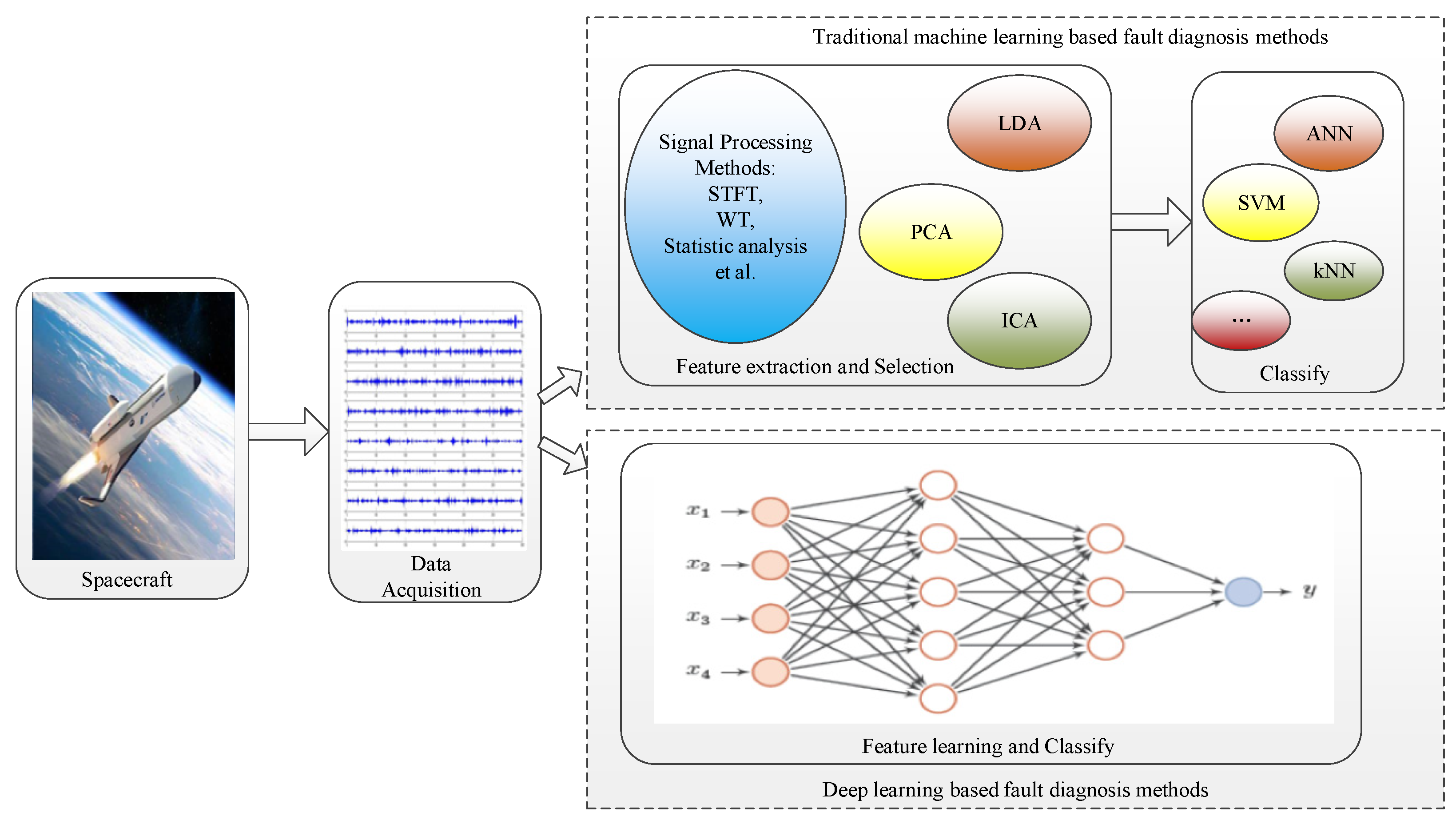
2.1. Fault Diagnosis Using Traditional Machine Learning

Data mining and traditional machine learning theories have been widely used in spacecraft fault diagnosis based on telemetry data. The procedures of shallow machine learning-based fault diagnosis methods are illustrated in Figure 1. Fault representations and characteristics were artificially extracted from telemetry data initially. Then, these sensitive representations were elaborately chosen to train diagnosis models, which can classify the fault types of spacecraft automatically.
Among all the machine learning-based fault diagnosis methods, expert systems are the most widely used approaches. If we can achieve sufficient experience and knowledge about the diagnosis task in advance, then expert system-based methods could be applied to identify the fault types in detail. I. Nakatani developed a diagnostic expert system for GEOTAIL satellite to enable operators with little knowledge to diagnose the overall state of satellite easily [4]. Z. Yang et al. [5] developed an expert system using fault tree analysis for gear box and achieved a precise and quick diagnosis result. Y. Guo et al. [6] proposed a novel fault diagnosis method, which used rules obtained through expert knowledge and characteristics of the system. D. V. Kodavade et al. [7] presented a universal fault diagnostic expert system method, which used object-oriented inference mechanism to improve efficiency. However, the performance of expert system-based fault diagnosis methods largely depends on the expert experience and knowledge, which is usually hard to be obtained and expressed. Once there is a fault problem that does not match the expert system, the diagnosis will fail. Moreover, the diagnosis knowledge set is hard to extend and modify, which is not suitable for modern complex instruments and apparatus in spacecraft with a huge number of sensors.
SVM is a computational learning algorithm and especially suitable for classification tasks. Compared to the artificial neural network, SVM-based fault diagnosis approaches are more explicable due to the fact that they are trained by minimizing the structural risk instead of the empirical risk. This interpretability is extremely crucial in the fault diagnosis of spacecraft. The SVM is generally used with other feature extraction methods. The New Operational SofTwaRe for Automatic Detection of Anomalies based on Ma-chine-learning and Unsupervised feature Selection (NOSTRADAMUS) by Centre National d’Etudes Spatiales (CNES) uses machine learning methods to extract characteristics and one-class SVM to classify anomalous data [8]. Sara K. Ibrahim et al. [9] used machine learning methods to analyze the performance of Egyptsat-1 satellite launched April 2007 and SVM to diagnose the fault models. M. L. Suo et al. [10] proposed an intelligent fault diagnosis method for the power system of satellites. It utilized fuzzy Bayes risk to generate an optimal feature subset and designed a classifier using SVM to identify faults. J. Shao et al. [11] used the immune genetic method to adjust the parameters of SVM regression, and then applied this method to detect the faults of a satellite attitude control system. In order to improve the diagnosis accuracy of SVM-based models, several improved models have been proposed.
ANN, which contains three types of components, i.e., input layer, hidden layers and output layers and has powerful fault pattern classification abilities, is considered to be the most commonly used algorithms in the field of fault diagnosis [12]. G. S. Naganathan et al. [13] proposed an ANN method for diagnosing the condition of the power transformer to predict the incipient faults as early as possible. Compared with ANN, the radial basis function (RBF) network is much easier to train [14]. Zhang et al. [15] proposed a hybrid model to choose the most useful and distinguished features and a weighted voting scheme based on the radial basis function (RBF) network to classify the features.
Traditional machine learning-based fault diagnosis requires artificial feature extraction, which leads to a huge labor cost. Furthermore, it is not suitable for the increasingly growing data volume due to the low generalization performance.

2.2. Fault Diagnosis Using Deep Learning

The recent advancements of deep learning, big data and cloud computing have led to major breakthroughs for multifarious problems including fault diagnosis tasks [16,17,18,19,20]. The deep learning methods shown in Figure 1 could learn discriminative patterns and representations from raw input signals and obtain higher diagnosis accuracy than other methods. The German Space Operation Center utilized the autoencoder to learn new feature vectors from the input layer and then detect anomalies in an Automated Telemetry Health Monitoring System (ATHMoS) [21]. As a modified model of RNN, Long Short-Term Memory (LSTM) shows a powerful ability to extract features from time series telemetry data. Hundman et al. demonstrated the viability and effectiveness of LSTM for predicting the telemetry data of spacecraft in NASA and proposed a dynamic threshold setting algorithm to enhance the detective accuracy of faults [22]. J. Chen et al. established a Bayesian LSTM model to conduct anomaly detection for the imbalanced satellite telemetry data [23]. M. Yuan et al. proposed an LSTM-based network to implement fault classification and remaining useful life estimation for an aero engine [24]. CNN is another essential deep model that is widely exploited in fault diagnosis and yields excellent performance. L. Wen et al. [25] developed a novel CNN network based on LeNet-5 to learn features from the two-dimensional signals and then diagnose faults.
The aforementioned deep learning methods are usually difficult to train due to gradient vanishing or exploding. Residual networks with skip connections, which could skip training from a few layers and transfer the original information directly to the output, are able to alleviate these issues. T. Zhang et al. [26] developed a fault diagnosis model that used STAC-tanh as an activated function to enhance the non-linear feature extraction ability and residual networks. Zhang et al. [27] proposed a residual learning algorithm to improve the information flow throughout the network and facilitate the network training.
In most engineering scenarios, the collected data contain many noises, and it is difficult to extract the fault characteristics directly from the time domain. Some researchers have revealed that useful features and representations will be more effortless to exploit and learn in a higher space [28]. Consequently, it is important to adopt advanced signal processing algorithms to transfer time domain data to frequency or time–frequency spectrum to learn more fault information. Zhao et al. [29] developed an improved deep residual network with dynamic wavelet packet coefficients to learn a set of features and promote the performance of fault diagnosis for a planetary gearbox.

3. Basics and Background

Since our proposed method is based on a deep residual convolutional neural network and short-time Fourier transform, the basic knowledge involved is briefly discussed first.

3.1. CNN and Deep Residual Networks

CNN, which has an excellent feature extraction capability and outstanding classification performance, has been widely used in the field of aerospace fault diagnosis [30,31]. A typical CNN is displayed in Figure 2, which consists of an input layer, convolutional layers, pooling layers, fully connected (FC) layers and an output layer. The raw time domain signals can be directly fed into the input layer, and the corresponding CNN is one dimensional (1D-CNN), while some signal processing techniques could be conducted to map the time domain data to various domains to improve and increase the diagnostic accuracy of the CNN. The output layer using the softmax activation function indicates the classification result of fault models.

3.1.1. Convolutional Layer

The convolutional layer is critical because it extracts features of input data. Compared to other deep models, CNN has two advantages: weight sharing and local connection, which greatly reduce the size of parameters and speed up training. Multiple convolutional kernels could be utilized in every convolutional layer to learn comprehensive features and representations. The equation of the convolutional layer can be described as
x l = σ ( W l x l 1 + b l )
where x l 1 and x l are the input and output, respectively. W l and b l represent the convolutional kernels and bias term, respectively. represents the convolutional operation, and σ denotes the activation function.

3.1.2. Pooling Layer

The pooling layer is often adopted to obviate redundancy and enable the learned feature to be more robust. The commonly used pooling layers contain max pooling and average pooling. In this study, we use max pooling layers, which select the maximum value of the pooled area. The mathematical operation of max pooling can be described as follows
y i j k = max ( m , n R i j ) x m n k
where y i j k is the output values, while x m n k denotes the value at the pooling area R i j around position ( m , n ) .

3.1.3. Batch Normalization (BN)

In order to accelerate the training procedure and avoid overfitting, several optimization strategies such as batch normalization (BN) [32] and Dropout are adopted. BN is a normalizing algorithm and can alleviate internal covariance shift. The mathematical model of BN is described as follows
μ = 1 N batch i = 1 N batch x i
σ 2 = 1 N batch i = 1 N batch ( x i μ ) 2
x ^ i = x i μ σ 2 + ε
y i = γ x ^ i + β
where x i denotes the input value, while x ^ i represents the result of the normalizing procedure,   N batch denotes the length of small batches of data, and μ and σ 2 denote the mean and variance of the input batch data, respectively. ε is a constant that is positive and very close to 0. y i denotes the output of the BN layer, and γ and β are the parameters that can be learned.

3.1.4. Residual Network

As the number of neural network layers increasingly grows to deepen, it becomes more and more difficult to train the CNN model. To address this problem, an improved model, called a residual network (Resnet), was proposed by K. He et al. [33]. Resnet adds a shortcut connection to the typical structure of the CNN, which could avoid the reduction in information. The shortcut connection structure is described in Figure 3, where x denotes the input and H ( x ) denotes the output; therefore, the Resnet aims to learn the difference between x and H ( x ) , i.e., F ( x ) = H ( x ) x . In this way, Resnet can facilitate the back propagation of errors and optimize the model’s parameters.
In the Resnet, the higher-level layer will obtain more information from the lower-level layers by using shortcut connections. In our fault diagnosis model, the Resnet is one of the most important modules. The Resnet usually contains several convolutional layers, BN layers and activated layers and then adds to the shortcut connection path to form a complete basic residual block.

3.2. Short-Time Fourier Transform

It is hard to extract fault features directly from the telemetry signals of an IMU due to the impact of noise. A solution is to transfer the data from the time domain to a frequency or time–frequency domain. The short-time Fourier transform (STFT) is a well-known method for time–frequency analysis. It is used to generate representations that capture both the local time and frequency features in the telemetry signals. The STFT uses the fixed-sized time-shifted window function h ( τ t ) , which has a user-defined time duration to obtain a transformation of the signal i ( t ) in the time domain. In other words, the STFT is generated by taking the Fourier transform of small durations of the original signal. In the continuous domain, STFT can be expressed as
S T F T { i ( t ) } = X ( τ , ω ) = + i ( t ) h ( t τ ) e j ω t d t
while in the discrete domain, STFT can be described as
X ( n , ω ) = m = + i ( m ) h ( m n ) e j ω m
where h ( n ) is the analysis window, which is assumed to be non-zero only between 0 and N 1 .
X ( n , k ) = X ( n , ω ) | ω = 2 π N k = m = + i ( m ) h ( m n ) e j 2 π N k m
In this work, the Hanning window function is adopted, and the length of the window is set to 64.

4. Proposed Method

In this section, we detail the proposed deep model with novel data preprocessing method to resolve the issues of fault diagnosis in IMU with a large volume of telemetry data. The framework is shown in Figure 4.

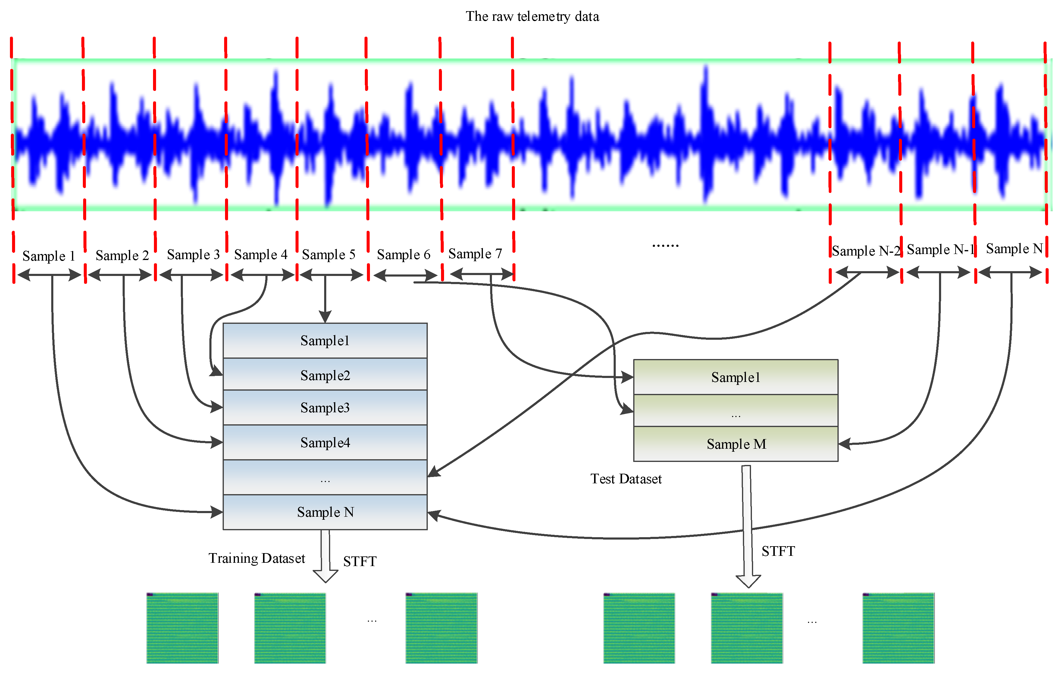
4.1. The Novel Data Acquisition and Preprocessing

In this study, the raw telemetry data are measured by inertial sensors in IMU and then transmitted to the ground center through microwaves. To promote the diagnosis accuracy, it is significant to preprocess the telemetry data before feeding them into the subsequent residual network. The novel preprocessing strategies proposed in this work include STFT, normalization and data augmentation.

4.1.1. Time–Frequency Transformation through STFT

The raw data are one-dimensional time sequences. We separate the time sequence into small slices with the length of 1024. Each slice denotes a sample. There are not overlaps between two slices. If the length of each original signal is L , then it can be divided into N samples, where N = floor ( L 1024 ) . We stochastically choose 80% of the entire slices as the training set, while the rest of slices form the test dataset. Figure 5 shows the data split method. Although the CNN can automatically extract features directly from the time domain of data, it is useful and effective to obtain the time–frequency spectrum with some more discriminative information than that in time domain [32]. Firstly, we adopt short-time Fourier transform (STFT) [34] to process the raw telemetry data in our method. The fault features are much easier to be distinguished than those in the time domain. The powerful characteristics of STFT promise to bring more discriminative features, which makes it easier for the subsequent residual network to classify fault categories.

4.1.2. Normalization

Generally speaking, the scales of different telemetry data in different channels vary widely due to different origins and characteristics. Normalization scales the data to be analyzed to a specific range such as [0.0, 1.0] or [−1, 1] to provide better results. It can enhance the following data processing and speed up the training of deep networks. The Z-score normalization is used to process the data because it can achieve better fault diagnosis than other normalization methods, e.g., Min–Max normalization and whitening normalization [17]. The Z-score normalization is shown as follows
x ^ i = x i μ σ
where μ represents the average value and σ represents the standard deviation of the training dataset. x i denotes the input data and x ^ i denotes the normalization result.

4.1.3. Date Augmentation

Deep neural networks usually need a lot of training samples to obtain ideal performance. However, the training samples, especially the faulty samples, are hard to obtain, and the training datasets are generally small. Data augmentation techniques can be utilized to extend the diversity and increase volume of training sets, improving the robustness of deep networks and avoiding overfitting.
As the original 1-D telemetry data have been transferred to 2-D time–frequency spectrum figures, data augmentation methods such as random scale and random crop for 2-D input data are finally applied to our method.
The random scale method multiplies the input data x with a value γ following the Gaussian distribution of N ( 1 ,   0.01 ) . The equation of random scale is shown as follows
x ¨ = * x
In the random crop, a binary sequence s , whose subsequence of random position is zero, covers partial input data x . The formulation of random crop can be described as follows
x ¨ = s x

4.2. Model Training

4.2.1. Improved Version of Activation Function

In the deep learning-based fault diagnosis model, the deep networks are usually used to extract discriminative representations, which has a significant influence on the performance of fault diagnosis. Moreover, the feature extraction and non-linear expression capabilities are mainly implemented by activation functions of each layer. According to different neural networks, various activation functions have been proposed and applied, among which Rectified Linear Unit (ReLU) [35] is one of the widely-adopted activation functions and has attracted widespread attention in deep models.
In essence, the ReLU returns 0 when the input is negative, while returns back to the same positive value if the input is non-negative. The mathematical function of ReLU is as follows
ReLU ( x ) = { 0   f o r   x < 0 x   f o r   x 0
Although ReLU can accelerate the convergence procedure and alleviate the vanishing gradient problem, the problem of “dead neurons” occurs when the neuron becomes stuck in the negative side and constantly outputs zero. Some improved versions have been developed to improve the performance of ReLU.
The Parameter ReLU (PReLU) introduces a set of learnable parameters γ i , which are different corresponding to different neurons of layers. A PReLU [36] is shown as follows
PReLU ( x ) = { γ i x   f o r   x < 0 x   f o r   x 0
The γ i could be learned using gradient backpropagation, and the non-linear ability of PReLU is highly flexible. PReLU not only allows different neurons to have different parameters, but also allows a group of neurons to share one parameter. Compared with ReLU activation function, the features learned by the PReLU are more discriminative and effective.

4.2.2. The Structure of Our Proposed Residual Network

Unlike the traditional CNN, residual networks first proposed by K. He et al. in 2016 [33] utilized a shortcut connection to allow lower-level features to be transferred to a higher-level layer directly.
Firstly, a basic residual block containing 2 convolutional layers (Conv), 2 batch normalization (BN) layers, 2 PReLU layers and a skip connection is constructed, which is shown in Figure 6. This basic residual block can not only promote the feature learning efficiency, but can also facilitate the extension of CNN and adjust the depth of network corresponding to the practical demand.
Then, the proposed residual network, which is responsible for extracting and learning discriminative features in the time–frequency spectrum, mainly contains convolutional layers, several basic residual blocks, maximum pooling layers, adaptive maximum pooling layer and fully connected layers, etc. The overall structure is shown in Figure 7. The wide convolutional layer adopts wide kernels to learn representations and further suppress the interference of noise [37]. The basic residual blocks are stacked to learn features, and the maximum pooling layers can reduce the parameters of the entire network. Finally, the learned high-level representations of input data are fed into the fully connected layers, which are mapped into different fault classes.

4.3. The Flow Chart of the Proposed Method

The flow chart of proposed model is shown in Figure 8, and the general procedure contains three steps: data acquisition and preprocessing, model training and model test.
(1) The telemetry data of IMU in spacecraft are obtained and divided into training dataset and test dataset without any overlap. The time–frequency spectrums are firstly obtained via STFT. Then, Z-score normalization is utilized to unify the data and the data augmentation tricks are adopted to make the dataset more diverse.
(2) The training dataset is fed into network to train the proposed model. The training process includes calculating the loss function, updating model parameters through Adam [38]. Once the model is well trained, the architecture and parameters are saved.
(3) The data preprocessing algorithm can be applied to the test dataset, and then test dataset are input to the trained model. Finally, the diagnosis results are obtained through the proposed model.

5. Experiments and Analysis

The proposed fault diagnosis algorithm is a data-driven method that diagnoses and analyzes the telemetry data sampled from the IMU. Aiming to validate the effectiveness and outstanding performance of the proposed model, we implemented experiments on public datasets similarly to many other literatures. The proposed deep learning model was implemented by using Pytorch with NVIDIA RTX 2080Ti GPU.

5.1. Case 1

5.1.1. Data Description and Preprocessing

Our proposed method was firstly conducted on the famous public dataset in the field of fault diagnosis provided by the Southeast University [39], which contains two sub-datasets, including the gear dataset and bearing dataset. This dataset is called the SEU dataset for short, and it is sampled from the Drivetrain Dynamics Simulator (DDS). As shown in Figure 9, the DDS consists of a motor, parallel gearbox and planetary gearbox.
According to the different rotating and speed configurations, there are two working conditions, which are 20 Hz–0 V and 30 Hz–2 V. There are five kinds of fault models for each kind of data, so the total number of types is 20 corresponding to different datasets. The dataset is shown in Table 1. In each file, there are eight rows of signals, and we use each row as a sub-dataset except the first row; therefore, there are seven sub-datasets denoted as SEU_A to SEU_G, respectively, in our experiment.
The raw data are divided into small pieces without any overlapping. Every slice has 1024 values and denotes a sample. Then each sample x i enters to the input of STFT. The Hanning window is selected, and the length of window is set to 64; therefore, after STFT, a 33 × 33 2-D spectrum image is generated for each sample. In order to make the subsequent residual network extract useful and discriminative features, the 33 × 33 spectrum images are adjusted to 330 × 330 by using resample.

5.1.2. Model Parameter Setting

The proposed model contains several trainable parameters including the values of convolutional kernels and bias, and many hyperparameters such as the number of convolutional layers, the number of basic residual blocks, the number of fully connected layers, etc. Appropriately setting the trainable parameters and hyperparameters greatly promotes the diagnosis performance of the deep model. The trainable parameters can be learned by optimizing loss functions, while it is difficult to effectively set the hyperparameters. In practical application scenarios, a feasible way to determine the final hyperparameters and their ranges is referring to expert experience and multiple experiments.
Considering the volume of the dataset, we use one wide convolutional layer, three basic residual blocks and three fully connected layers to construct the backbone of our model. The number of neurons in the output fully connected layer is equal to the numbers of fault types. The structure of the proposed method is shown in Figure 7 and the parameters are detailed in Table 2.
The Adam optimizer is used and the size of the mini-batch is 32. The learning rates are 0.001. To avoid overfitting, the dropout trick is applied in the fully connected layers, and the dropout rate is 0.5. To avoid randomness, every experiment is repeated six times, and the average of classification accuracies is taken as the final results.

5.1.3. Comparison Methods

To prove and validate the effectiveness and outstanding performance of the proposed fault diagnosis methods over other methods, we used several state-of-the-art approaches to compare the experiment results, including AE [40], DAE [41], CNN [25], AlexNet [42] and LSTM [22]. All the networks’ architectures of the comparison methods are shown in Table 3.
Autoencoder (AE), which contains an encoder and a decoder, is an unsupervised deep learning method for feature extraction. The encoder is used to extract hidden representations of input data, while the decoder attempts to reconstruct the original input data from the hidden representations learned by the encoder. In this study, the encoder of AE contained five convolutional layers with BN and two fully connected layers, and the relevant decoder contained two fully connected layers and five transposed convolutional layers. A denoising autoencoder, which is a derivative of the AE, has the same network structure with the AE in this study.
The CNN used was constructed with two continuous convolutional layers followed by a max pool layer, and then three continuous convolutional layers followed by a max pool layer. There were three fully connected layers at the end of the model. AlexNet was proposed by Krizhevsky A. in 2012, and it is a derivative of CNN, which contains five convolutional layers, three max pool layers and three fully connected layers.
The LSTM network is a variant of RNN that adopts modified units instead of standard units. It has a powerful feature extraction ability in time series and has become popular in fault diagnosis to extract fault representations. The LSTM model used in this paper contained three LSTM layer and three fully connected layers.
In addition, all baseline methods used two-dimensional (2-D) time–frequency images as input, which were processed by using the method detailed in Section 4.2, and each convolutional layer was followed by a BN layer to speed up the convergence of the network. Moreover, to guarantee the fairness of comparison, the comparison methods attempted to use the same hyperparameters adopted by the proposed method. In addition to that, the softmax activation function was adopted in the last layer, while the rest of the layers used PReLU as an activation function if necessary.

5.1.4. Results’ Analysis

To quantitatively measure the performance of various approaches, classification accuracy, defined as below, was used.
Accuracy = | x : x D t e s t y ^ t e s t = y t e s t | | x : x D t e s t |
where D t e s t represents the test dataset, y t e s t is the true label and y ^ t e s t is the predicted label.
The experiments were conducted six times for each algorithm, and the mean accuracy was calculated. The classification accuracies in the SEU datasets are presented in Table 4. Some conclusions can be drawn as follows:
(1) The proposed approach achieved the best performance across all the datasets.
(2) In all seven datasets, the accuracies of the proposed approach were larger than 93%, and the average accuracy was 97.16%, which was 11.17%, 4.87%, 23.92%, 9.66% and 14.42% higher than the AE, DAE, CNN, AlexNet and LSTM, respectively. It also indicates that our proposed method can diagnose the fault types of SEU datasets well.
(3) The average accuracy of the DAE (92.29%) was superior to the AE (85.99%) due to the fact that the DAE takes an input mixed with noise and is trained to reconstruct the pure type of the input.
(4) LSTM achieved an overall average accuracy of 82.74%, yielding 9.5% improvements compared to the CNN, which shows that LSTM can extract more discriminative features than CNN.
The histogram of diagnosis accuracy for various methods in the seven SEU datasets is shown in Figure 10.

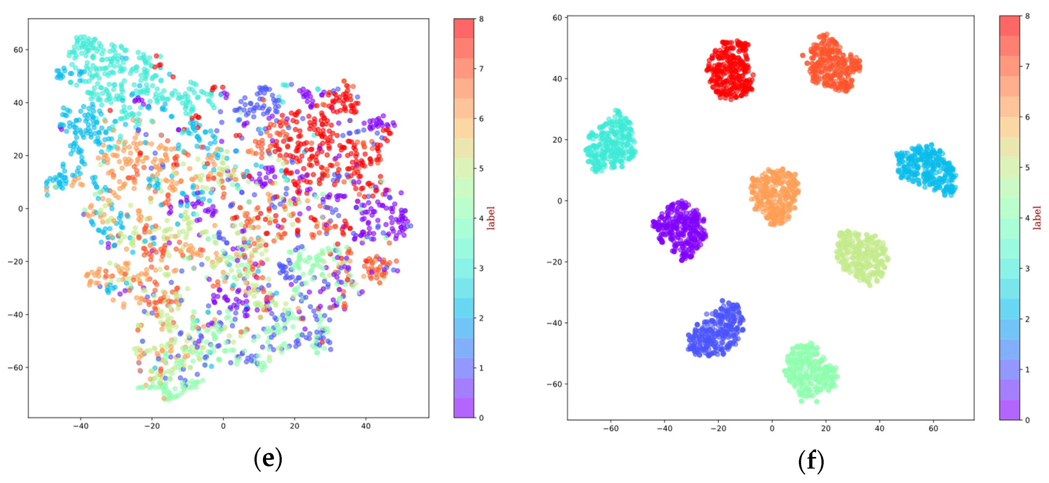
5.1.5. Visualization Analysis

In order to comprehend the predominant performance of the proposed approach more intuitively, the confusion matrix and t-distributed Stochastic Neighbor Embedding (t-SNE) technologies were utilized to visualize the results. The confusion matrixes of the diagnosis results in the SEU_B dataset are detailed in Figure 11.
Figure 11 shows the confusion matrixes of the diagnostic results in the SEU_B dataset for AE, DAE, CNN, AlexNet, LSTM and our proposed method, respectively. From Figure 11, we can conclude that the proposed approach correctly classified 14 fault types except for fault labels 2, 7, 10, 15, 17 and 19. In fault type 15, the proposed method misclassified six samples. Combined with the results exhibited in Table 4, the proposed model outperformed other baseline methods in classifying fault types for the SEU dataset.
In order to understand and visualize the features learned by the models, t-SNE technology, which can compress the high-dimensional features into two-dimensional space, was adopted to visualize the features from the output layer of the model. Taking the diagnosis task for the SEU_B dataset, for example, Figure 12 shows the learning by AE, DAE, CNN, AlexNet, LSTM and our proposed method, respectively. The different colors in Figure 12 represent the different fault types of samples, and the coordinate value of every point denotes the location of the according point in the two-dimensional domain.
As shown in Figure 12, among all the baseline methods, the CNN shown in Figure 12c exhibits the worst cluster performance, with a large number of points of different fault models overlapping, while points that have the same fault types are not gathered together. The results of the AE shown in Figure 12a and the DAE shown in Figure 12b indicate that they perform better than CNN and LSTM, shown in Figure 12c,e, respectively. However, in Figure 12f, our proposed method separates nearly all 20 fault types, and only a few overlaps can be observed. Moreover, the distance between any two clusters is relatively far away, which indicates that the proposed approach has a better ability to identify the fault types and, consequently, has a much higher classification accuracy.

5.2. Case 2

5.2.1. Data Description

Another dataset provided by the University of Connecticut (UoC) [43] was also used. The UoC dataset contains nine fault models, including root crack, spalling, missing tooth, five chipping tips with different levels of severity and a normal condition.

5.2.2. Results’ Analysis

The baseline methods were still AE, DAE, CNN, AlexNet and LSTM. The network architectures and parameter setting were similar to Case 1.
The accuracies are presented in Table 5. The accuracy of the proposed algorithm was 77.02%, which was 27.25% higher than the second-performing method, i.e., DAE, indicating that the proposed approach can not only extract discriminative features but can also classify the fault types well. To compare the performance of the ReLU and PReLU activation functions, an ablation study was conducted, and the results are shown in the last two columns of Table 5. It indicates that using the PReLU activation function in the proposed model can obtain a higher diagnostic accuracy (77.02%) than using the ReLU activation function (75.17%).

5.2.3. Visualization Analysis

The features learned from the output layer of the UoC datasets are shown in Figure 13. The AE, DAE and our proposed method could separate the features well, but the CNN, AlexNet and LSTM could not separate the points of different types. In Figure 13c–e, a large number of fault models overlap and mix together, making it extremely hard to classify them, while in Figure 13f, different fault models are well separated and far away from each other. Moreover, points of the same fault type are concentrated together. Hence, the proposed method can separate the features better than other baseline approaches and has a higher accuracy.

6. Conclusions

In order to learn discriminative fault characteristics and representations and promote the diagnosis performance of IMU in spacecraft, this study proposes a novel data preprocessing algorithm and a diagnosis network based on deep learning. Firstly, a novel data preprocessing method for the telemetry data is proposed. This method uses STFT to acquire time–frequency spectrum images of input samples, and the Z-score normalization and data augmentation techniques are also exploited to facilitate the training of the subsequent deep model and avoid a gradient vanishing problem. Then, a basic residual block with a shortcut connection is proposed and several of these blocks are stacked to construct a deep fault diagnosis model. Finally, to enhance the non-linear feature extraction ability of the proposed model, the activation function is improved by using PReLU instead of the traditional ReLU. Experimental results indicate that the proposed model has good fault features’ extraction ability and exceeds other state-of-the-art models in terms of classification accuracy.
At present, our work is based on the assumption that the training and test data should follow the identical distribution. Unfortunately, this hypothesis does not always hold in most application scenarios. For example, in the area of machines’ fault diagnosis, the training dataset and test dataset are often collected in different working conditions, which results in a shift in data distribution. Therefore, transfer learning (TL)-based fault diagnosis approaches will be our research emphases in the future.

Author Contributions

Conceptualization and writing, G.X.; methodology, J.M.; software, L.C.; validation, X.H. All authors have read and agreed to the published version of the manuscript.

Funding

The National Basic Scientific Research under Grant No. JCKY2016203A003. The Equipment Pre-research Key Laboratory Funds under Grant No. 61425010102.

Institutional Review Board Statement

Not applicable.

Informed Consent Statement

Not applicable.

Data Availability Statement

The datasets generated and/or analyzed during the current study are available from the corresponding author on reasonable request.

Conflicts of Interest

The authors declare no conflict of interest.

References

  1. Tazartes, D. An historical perspective on inertial navigation systems. In Proceedings of the 2014 international symposium on inertial sensors and systems (ISISS), Laguna Beach, CA, USA, 25–26 February 2014; pp. 1–5. [Google Scholar]
  2. Wang, L.; Li, K.; Zhang, J.; Ding, Z.X. Soft Fault Diagnosis and Recovery Method Based on Model Identification in Rotation FOG Inertial Navigation System. IEEE Sens. J. 2017, 17, 5705–5716. [Google Scholar] [CrossRef]
  3. Lu, S.; Zhou, W.; Huang, J.; Lu, F.; Chen, Z. A Novel Performance Adaptation and Diagnostic Method for Aero-Engines Based on the Aerothermodynamic Inverse Model. Aerospace 2022, 9, 16. [Google Scholar] [CrossRef]
  4. Nakatani, I.; Hashimoto, M.; Nishigori, N.; Mizutani, M. Diagnostic expert system for scientific satellite. Acta Astronaut. 1994, 34, 101–107. [Google Scholar] [CrossRef]
  5. Yang, Z.-L.; Wang, B.; Dong, X.-H.; Liu, H. Expert System of Fault Diagnosis for Gear Box in Wind Turbine. Syst. Eng. Procedia 2012, 4, 189–195. [Google Scholar]
  6. Guo, Y.; Wang, J.; Chen, H.; Li, G.; Huang, R.; Yuan, Y.; Ahmad, T.; Sun, S. An expert rule-based fault diagnosis strategy for variable refrigerant flow air conditioning systems. Appl. Therm. Eng. 2019, 149, 1223–1235. [Google Scholar] [CrossRef]
  7. Kodavade, D.V.; Apte, S.D. A Universal Object-Oriented Expert System Frame Work for Fault Diagnosis. Int. J. Intell. Sci. 2012, 2, 63–70. [Google Scholar] [CrossRef]
  8. Fuertes, S.; Picart, G.; Tourneret, J.Y.; Chaari, L.; Ferrari, A.; Richard, C. Improving Spacecraft Health Monitoring with Automatic Anomaly Detection Techniques. In Proceedings of the 14th International Conference on Space Operations, Daejeon, Korea, 16–20 May 2016; p. 2430. [Google Scholar]
  9. Ibrahim, S.K.; Ahmed, A.; Zeidan, M.A.E.; Ziedan, I.E. Machine Learning Techniques for Satellite Fault Diagnosis. Ain Shams Eng. J. 2020, 11, 45–56. [Google Scholar] [CrossRef]
  10. Suo, M.; Zhu, B.; An, R.; Sun, H.; Xu, S.; Yu, Z. Data-driven fault diagnosis of satellite power system using fuzzy Bayes risk and SVM. Aerosp. Sci. Technol. 2019, 84, 1092–1105. [Google Scholar] [CrossRef]
  11. Shao, J.; Zhang, Y. Fault Diagnosis Based on IGA-SVMR for Satellite Attitude Control System. Appl. Mech. Mater. 2014, 494–495, 1339–1342. [Google Scholar]
  12. Liu, R.; Yang, B.; Zio, E.; Chao, X. Artificial intelligence for fault diagnosis of rotating machinery: A review. Mech. Syst. Signal Process. 2018, 108, 33–47. [Google Scholar] [CrossRef]
  13. Naganathan, G.; Senthilkumar, M.; Aiswariya, S.; Muthulakshmi, S.; Riyasen, G.S.; Priyadharshini, M.M. Internal fault diagnosis of power transformer using artificial neural network. Mater. Today Proc. 2021; in press. [Google Scholar]
  14. Narendra, K.G.; Sood, V.K.; Khorasani, K.; Patel, R. Application of a radial basis function (RBF) neural network for fault diagnosis in a HVDC system. IEEE Trans. Power Syst. 1998, 13, 177–183. [Google Scholar] [CrossRef]
  15. Zhang, K.; Li, Y.; Scarf, P.; Ball, A. Feature selection for high-dimensional machinery fault diagnosis data using multiple models and radial basis function networks. Neurocomputing 2011, 74, 2941–2952. [Google Scholar] [CrossRef]
  16. Peng, Z.; Dong, K.; Wang, Y.; Huang, X. A Fault Diagnosis Model for Coaxial-Rotor Unit Using Bidirectional Gate Recurrent Unit and Highway Network. Machines 2022, 10, 313. [Google Scholar] [CrossRef]
  17. Zhao, Z.; Li, T.; Wu, J.; Sun, C.; Wang, S.; Yan, R.; Chen, X. Deep learning algorithms for rotating machinery intelligent diagnosis: An open source benchmark study. ISA Trans. 2020, 107, 224–255. [Google Scholar] [CrossRef]
  18. Khan, S.; Yairi, T. A review on the application of deep learning in system health management. Mech. Syst. Signal Process. 2018, 107, 241–265. [Google Scholar] [CrossRef]
  19. Nguyen, V.-C.; Hoang, D.-T.; Tran, X.-T.; Van, M.; Kang, H.-J. A Bearing Fault Diagnosis Method Using Multi-Branch Deep Neural Network. Machines 2021, 9, 345. [Google Scholar] [CrossRef]
  20. Jiao, J.; Zhao, M.; Lin, J.; Liang, K. A comprehensive review on convolutional neural network in machine fault diagnosis. Neurocomputing 2020, 417, 36–63. [Google Scholar] [CrossRef]
  21. Omeara, C.; Schlag, L.; Faltenbacher, L.; Wickler, M. ATHMoS: Automated Telemetry Health Monitoring System at GSOC using Outlier Detection and Supervised Machine Learning. In Proceedings of the 14th International Conference on Space Operations, Daejeon, Korea, 16–20 May 2016; p. 2347. [Google Scholar]
  22. Hundman, K.; Constantinou, V.; Laporte, C.; Colwell, I.; Soderstrom, T. Detecting Spacecraft Anomalies Using LSTMs and Nonparametric Dynamic Thresholding. In KDD ‘18: Proceedings of the 24th ACM SIGKDD International Conference on Knowledge Discovery & Data Mining; ACM: New York, NY, USA, 2018; pp. 387–395. [Google Scholar]
  23. Chen, J.; Pi, D.; Wu, Z.; Zhao, X.; Pan, Y.; Zhang, Q. Imbalanced satellite telemetry data anomaly detection model based on Bayesian LSTM. Acta Astronaut. 2021, 180, 232–242. [Google Scholar] [CrossRef]
  24. Yuan, M.; Wu, Y.; Lin, L. Fault diagnosis and remaining useful life estimation of aero engine using LSTM neural network. In Proceedings of the 2016 IEEE International Conference on Aircraft Utility Systems (AUS), Beijing, China, 10–12 October 2016; pp. 135–140. [Google Scholar]
  25. Wen, L.; Li, X.; Gao, L.; Zhang, Y. A New Convolutional Neural Network-Based Data-Driven Fault Diagnosis Method. IEEE Trans. Ind. Electron. 2018, 65, 5990–5998. [Google Scholar] [CrossRef]
  26. Zhang, T.; Liu, S.; Wei, Y.; Zhang, H. A novel feature adaptive extraction method based on deep learning for bearing fault diagnosis. Measurement 2021, 185, 110030. [Google Scholar] [CrossRef]
  27. Zhang, W.; Li, X.; Ding, Q. Deep residual learning-based fault diagnosis method for rotating machinery. ISA Trans. 2019, 95, 295–305. [Google Scholar] [CrossRef] [PubMed]
  28. Ding, X.; He, Q. Energy-uctuated multiscale feature learning with deep ConvNet for intelligent spindle bearing fault diagnosis. IEEE Trans. Instrum. Meas. 2017, 66, 9261935. [Google Scholar] [CrossRef]
  29. Zhao, M.; Kang, M.; Tang, B.; Pecht, M. Deep Residual Networks With Dynamically Weighted Wavelet Coefficients for Fault Diagnosis of Planetary Gearboxes. IEEE Trans. Ind. Electron. 2018, 65, 4290–4300. [Google Scholar] [CrossRef]
  30. Shao, X.; Kim, C.-S. Unsupervised Domain Adaptive 1D-CNN for Fault Diagnosis of Bearing. Sensors 2022, 22, 4156. [Google Scholar] [CrossRef] [PubMed]
  31. JJiang, G.; He, H.; Yan, J.; Xie, P. Multiscale Convolutional Neural Networks for Fault Diagnosis of Wind Turbine Gearbox. IEEE Trans. Ind. Electron. 2019, 66, 3196–3207. [Google Scholar] [CrossRef]
  32. Ioffe, S.; Szegedy, C. Batch normalization: Accelerating deep network training by reducing internal covariate shift. In Proceedings of the 32nd International Conference on Machine Learning (ICML 2015), Lille, France, 6–11 July 2015; Volume 1, pp. 448–456. [Google Scholar]
  33. He, K.; Zhang, X.; Ren, S.; Sun, J. Identity Mappings in Deep Residual Networks. In European Conference on Computer Vision; Springer: Cham, Switzerland, 2016; pp. 630–645. [Google Scholar]
  34. Hasan, M.J.; Islam, M.M.; Kim, J.M. Multi-sensor fusion-based time-frequency imaging and transfer learning for spherical tank crack diagnosis under variable pressure conditions. Measurement 2021, 168, 108478. [Google Scholar] [CrossRef]
  35. Nair, V.; Hinton, G.E. Rectified linear units improve restricted boltzmann machines. In Proceedings of the International Conference on Machine Learnin, Haifa, Israel, 21–24 June 2010; pp. 807–814. [Google Scholar]
  36. He, K.; Zhang, X.; Ren, S.; Sun, J. Delving deep into rectifiers: Surpassing human-level performance on imagenet classification. In Proceedings of the IEEE International Conference on Computer Vision, Santiago, Chile, 7–13 December 2015; pp. 1026–1034. [Google Scholar]
  37. Song, X.; Cong, Y.; Song, Y.; Chen, Y.; Liang, P. A bearing fault diagnosis model based on CNN with wide convolution kernels. J. Ambient. Intell. Humaniz. Comput. 2021, 13, 4041–4056. [Google Scholar] [CrossRef]
  38. Kingma, D.; Ba, J. Adam: A method for stochastic optimization. In Proceedings of the International Conference on Learning Representations, San Diego, CA, USA, 7–9 May 2015. [Google Scholar]
  39. Liang, H.; Cao, J.; Zhao, X. Multi-scale dynamic adaptive residual network for fault diagnosis. Measurement 2021, 188, 110397. [Google Scholar] [CrossRef]
  40. Kong, X.; Mao, G.; Wang, Q.; Ma, H.; Yang, W. A multi-ensemble method based on deep auto-encoders for fault diagnosis of rolling bearings. Measurement 2020, 151, 107132. [Google Scholar] [CrossRef]
  41. Lu, C.; Wang, Z.; Qin, W.; Ma, J. Fault diagnosis of rotary machinery components using a stacked denoising autoencoder-based health state identification. Signal Process. 2017, 130, 377–388. [Google Scholar] [CrossRef]
  42. Shi, X.; Cheng, Y.; Zhang, B.; Zhang, H. Intelligent fault diagnosis of bearings based on feature model and Alexnet neural network. In Proceedings of the 2020 IEEE International Conference on Prognostics and Health Management (ICPHM), Detroit, MI, USA, 8–10 June 2020. [Google Scholar]
  43. Cao, P.; Zhang, S.; Tang, J. Gear Fault Data. Available online: https://figshare.com/articles/dataset/Gear_Fault_Data/6127874/1 (accessed on 15 July 2022).
Figure 1. Machine learning- and deep learning-based fault diagnosis methods.
Machines 10 00851 g001
Figure 2. Structure of CNN.
Machines 10 00851 g002
Figure 3. The architecture of residual network.
Machines 10 00851 g003
Figure 4. The framework of the proposed fault diagnosis method.
Machines 10 00851 g004
Figure 5. The data splitting method.
Machines 10 00851 g005
Figure 6. The structure of basic residual block.
Machines 10 00851 g006
Figure 7. The overall structure of proposed neural network.
Machines 10 00851 g007
Figure 8. The flow chart of proposed model.
Machines 10 00851 g008
Figure 9. The test rig of DDS.
Machines 10 00851 g009
Figure 10. Histogram of diagnosis accuracies for different algorithms.
Machines 10 00851 g010
Figure 11. The confusion matrixes of the diagnosis results in SEU_B dataset. (a) Confusion matrix for AE, (b) confusion matrix for DAE, (c) confusion matrix for CNN, (d) confusion matrix for AlexNet, (e) confusion matrix for LSTM, (f) confusion matrix for proposed method.
Machines 10 00851 g011aMachines 10 00851 g011b
Figure 12. Visualization of features from the output layer for SEU_B dataset: (a) visualization results for AE, (b) visualization results for DAE, (c) visualization results for CNN, (d) visualization results for AlexNet, (e) visualization results for LSTM, (f) visualization results for proposed method.
Machines 10 00851 g012aMachines 10 00851 g012b
Figure 13. Visualization of features from the output layer for UoC dataset: (a) visualization results for AE, (b) visualization results for DAE, (c) visualization results for CNN, (d) visualization results for AlexNet, (e) visualization results for LSTM, (f) visualization results for proposed method.
Machines 10 00851 g013aMachines 10 00851 g013b
Table 1. The details of SEU.
LabelDatasetFault TypeWorking ConditionLabelDatasetFault TypeWorking Condition
0BearingBall20 Hz–0 V10GearChipped20 Hz–0 V
1BearingCombination20 Hz–0 V11GearHealth20 Hz–0 V
2BearingHealth20 Hz–0 V12GearMiss20 Hz–0 V
3BearingInner20 Hz–0 V13GearRoot20 Hz–0 V
4BearingOuter20 Hz–0 V14GearSurface20 Hz–0 V
5BearingBall30 Hz–2 V15GearChipped30 Hz–2 V
6BearingCombination30 Hz–2 V16GearHealth30 Hz–2 V
7BearingHealth30 Hz–2 V17GearMiss30 Hz–2 V
8BearingInner30 Hz–2 V18GearRoot30 Hz–2 V
9BearingOuter30 Hz–2 V19GearSurface30 Hz–2 V
Table 2. Hyperparameters of the proposed method.
No.LayerOutput ChannelsKernel SizeStridePaddingActivation Function
1Conv2d 116 13 × 131YesPReLU
2Maxpool 1/ 2 × 22No/
3Basic residual block 164 3 × 31YesPReLU
4Basic residual block 2128 3 × 31Yes PReLU
5Basic residual block 3256 3 × 31YesPReLU
10AdaptiveMaxpool///No/
11FC 1////PReLU
12Output layer////Softmax
Table 3. The architecture of comparison methods.
AEDAECNNAlexNetLSTMProposed Method
Input
5 Conv
2 FC
2 FC
5 ConvT
Conv
Input
5 Conv
2 FC
2 FC
5 ConvT
Conv
Input
2 Conv
1 Maxpool
3 Conv
1 Maxpool
3 FC
Input
1 Conv
1 Maxpool
1 Conv
1 Maxpool
3 Conv
1 Maxpool
3 FC
Input
3 LSTM
3 FC
Input
1 Conv
1 Maxpool
3 basic residual blocks
1 Maxpool
3 FC
Table 4. Accuracy (%) of different algorithms for SEU dataset.
DatasetAEDAECNNAlexNetLSTMProposed Method
SEU_A95.3496.8183.3394.3690.6998.77
SEU_B84.5693.6361.0287.9979.1796.81
SEU_C97.3095.8384.8088.4889.9599.02
SEU_D93.3894.1289.9585.0581.8698.04
SEU_E89.4694.8569.3689.7183.5899.51
SEU_F73.5381.1363.2484.8079.1794.12
SEU_G68.3889.7161.0382.1174.7593.87
Average85.9992.2973.2487.5082.7497.16
Table 5. Accuracy (%) for methods in UoC dataset.
DatasetAEDAECNNAlexNetLSTMProposed Method
(ReLU)
Proposed Method
(ReLU)
UoC47.3449.7732.7237.1434.5575.1777.02
Publisher’s Note: MDPI stays neutral with regard to jurisdictional claims in published maps and institutional affiliations.

