Affine Layer-Enabled Transfer Learning for Eye Tracking with Facial Feature Detection in Human–Machine Interactions

Abstract

Eye tracking is an important technique for realizing safe and efficient human–machine interaction. This study proposes a facial-based eye tracking system that only relies on a non-intrusive, low-cost web camera by leveraging a data-driven approach. To address the challenge of rapid deployment to a new scenario and reduce the workload of the data collection, this study proposes an efficient transfer learning approach that includes a novel affine layer to bridge the gap between the source domain and the target domain to improve the transfer learning performance. Furthermore, a calibration technique is also introduced in this study for model performance optimization. To verify the proposed approach, a series of comparative experiments are conducted on a designed experimental platform to evaluate the effects of various transfer learning strategies, the proposed affine layer module, and the calibration technique. The experiment results showed that the proposed affine layer can improve the model’s performance by $7\%$ (without calibration) and $4\%$ (with calibration), and the proposed approach can achieve state-of-the-art performance when compared to the others.

1. Introduction

In the context of Industry 5.0, artificial intelligence (AI) methods have shown tremendous progress, which indicates that intelligent agents have been widely applied to multiple areas, such as collaborative robots [1,2] and intelligent vehicles [3,4,5,6,7], which need humans to co-operate with the automation systems. Many advanced technologies, including intelligent delivery robots, have also been released [8]. Although these intelligent robots are autonomous, they are still required to be supervised remotely by an operator in order to effectively take over in distinct situations. This indicates that the coexistence and collaboration of human and intelligent agents would be a crucial concern [9,10]. This design requires agents to be able to understand human behavior and intention and users to be aware of the agent’s performance limits [11,12,13,14,15]. This way, both can coexist safely and use their advantages to collaborate for the completion of specific tasks.

In multi-modal human–human interaction [16,17,18], the gaze is an important signal of information that can be used to analyze and understand the attention and intention of the people, and the same is true for human–machine interaction [19,20,21]. There are two different kinds of research about the human gaze: gaze estimation [22] and eye tracking [23]. The first assesses the direction of the gaze, while the last directly estimates the focused area (where one is looking at). Eye tracking has been applied to many areas, through the visual system, psychology, psycholinguistics, marketing, product design, and rehabilitative and assistive applications. Different applications have different types of sensors and devices. This study focuses on the eye tracking system with a non-intrusive, low-cost sensor.

Generally, eye tracking requires a specialized device known as the eye tracker. Most modern eye trackers are equipped with either one or two cameras and one or more infrared light sources, such as the Tobii Eye Tracker and SMI REDn. The infrared light is used to illuminate the face and eyes to create a corneal reflection, while the camera captures the face and eyes. Eye trackers compute the point of gaze by comparing the location of the pupil to the location of the corneal reflection in the camera image. The types of eye-tracking systems can be divided into three categories based on freedom for the user [24,25]: (1) Wearable eye tracker, which is mounted on the head of the user, and usually mimics the appearance of glasses. They are typically equipped with a scene camera to provide a view of what the user is looking at. (2) Mounted eye tracker, which generally employs one or more infrared sensors that are placed at a fixed location in front of the user, and the user can freely move in a certain section of space. (3) Head-restricted eye tracker, which constitutes a tower-mounted eye tracker, or a remote eye tracker with a chin rest. Tower-mounted eye trackers restrict both the chin and the head and film the eyes from above. By contrast, the mounted eye tracker is less intrusive and easier to use, and this study aims to develop this type of eye tracking system using a web camera.

Eye tracking has been studied over a few decades, and it continues to be an interesting research topic. Recently, there has been rapid development in data-driven eye tracking technology, which has attracted more attention, especially the camera-based appearance eye tracking method. Zhang et al. [26] proposed a convolutional neural network (CNN) with spatial weights applied to the feature maps to flexibly suppress or enhance information in different facial regions. They used the face region without considering the position of the face in the frontal image. TabletGaze [27] collected an unconstrained gaze dataset of tablet users who vary in race, gender, and glasses, called the Rice TabletGaze dataset. However, the dataset only consists of 35 fixed gaze locations. Driven by the collected data, they proposed a multi-level Histogram of Oriented Gradient feature and a random forests regressor to estimate the gaze position. Li et al. [28] presented a long-distance gaze estimation method, where they used one eye tracker to obtain the ground truth and another to train a camera for eye tracking. iTracker [29] collected the first large-scale eye tracking dataset, which captured data from over 1450 people, consisting of almost 2.5 M frames. Using the collected dataset, they trained a CNN that achieved a significant reduction in error, while running in real-time, as compared to previous approaches. In this study, the iTracker is used as a pre-trained feature extractor. Hu et al. [30] proposed an eye tracking method through a dual-view camera, which combined the saliency map and semantic information of a scene, whereas the TurkerGaze [31] combined the saliency map and support vector regression to regress the position of the eye. Simultaneously, Yang et al. [32] proposed a non-intrusive, dual-camera-based calibrated gaze mapping system, which used the orthogonal least squares algorithm to establish the correspondence relation. From the related works, it can be observed that eye tracking is highly conditional to the sensor and application scene. If re-collected, obtaining a large dataset for the new scenario is a laborious challenge. Hence, this study aims to propose a low-cost, efficient eye-tracking solution that can leverage the transfer learning to rapidly deploy to a new application.

There are three main contributions of this study. First, a low-cost eye gaze tracking system is presented to promote it to be utilized in more human–machine collaboration applications. Second, an efficient transfer learning approach with a novel affine layer is proposed to accelerate deployment into a new scenario, reduce data collection workload, and improve model performance. Third, a calibration step is introduced to optimize model performance and increase robustness when dealing with various users.

2. Materials and Methods

2.1. Overview

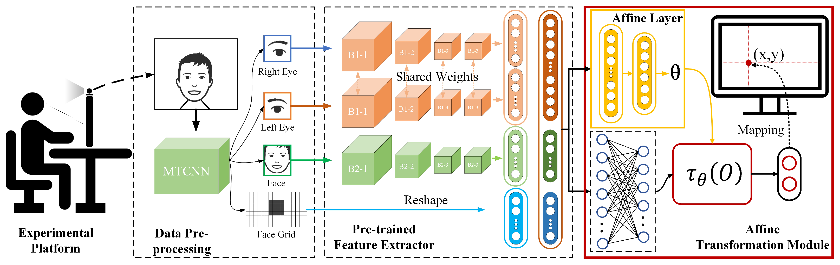
The main purpose of this study is to build an eye tracking system in real-time, employing only a web camera, where the computer screen is chosen as the application platform. The reasonable solution should be a data-driven method utilizing a CNN model. The lack of a suitable dataset that has enough variety of subjects poses a challenge. Hence, transfer learning was leveraged to conquer this problem based on a phone-oriented eye tracking model, iTracker. To achieve the best transfer performance and keep the low calculation load, several transfer learning protocols were explored, and an affine layer module is proposed to assist the transfer learning of similar domains.

The overall framework of the proposed approach is shown in Figure 1 and Algorithm 1. The experimental platform includes three objects: user, computer screen and web-camera. The web-camera could capture the RGB image of the user, while a face detection module was used to detect the bounding box and key points of the face. After the pre-processing, the raw image was transformed into four feature maps: right eye, left eye, face and face grid. Then a pre-trained model was leveraged to extract the facial features. These facial feature vectors were entered into the proposed affine layer module and the output layer, respectively. Finally, the eye position was calculated using the output transformation module. A calibration step was designed to fine-tune the trained model and optimize its performance.

Algorithm 1. Eye tracking pipeline

1: Initialization: Model calibration via 13 fixed dots

2: repeat

3:    Face detection

4:    Detection pre-processing: left and right eye image, face image, face grid

5:    Eye fixation estimation by using the proposed AffNet

6: until Program exit

2.2. Data Pre-Processing

For eye tracking, the head pose and eye gaze are the most relevant features. To let the model focus on these indicators, a face detector can be used to extract the face and eyes instead of the raw image being used as the input maps. The current face detection module is very mature and has been deployed on many successful commercial applications. In this study, MTCNN [34] was used in the face detection module, which leverages a cascaded architecture with carefully designed deep CNNs to predict face and landmark location in a coarse-to-fine manner. Its accuracy achieves excellency on the FDDB and WIDER FACE benchmarks for face detection and AFLW benchmark for face alignment while maintaining real-time performance. Cropping the face and eyes can also let the model accommodate the different kinds of backgrounds. Due to the gaze direction being a three-dimensional vector, the relative position of the user to the camera is also important and should be considered. Therefore, the face grid was used to reflect the relative XYZ position of the face. The raw image was divided into several grids, such that the corresponding grids of the face area were 1 and the others were 0. Finally, it was reshaped into a one-dimension vector.

2.3. Feature Extraction

Currently, the building and training of a new deep learning model turns out to be very high cost and time-consuming, and sometimes difficult to achieve due to the lack of a suitable dataset. Hence, the prosperity of deep-learning benefits from the emergence of large-scale data sets. The ImageNet dataset [35] is a very large collection of human-annotated images, used for the development of computer vision algorithms, which has led to the creation of multiple milestone model architectures and techniques in the intersection of computer vision and deep learning. There was no well-matching large dataset that could be used for the research of this study and collection of a new dataset with millions of samples is very laborious, which is why we were inspired by transfer learning and discovered a new solution.

Transfer learning is a popular approach in deep learning where pre-trained models are used as the starting point for the computer vision and natural language processing tasks, given the vast computer and time resources required to develop a new neural network model for these problems. Fortunately, there is a large-scale dataset for eye tracking through the phone, iTracker, which contains data from over 1450 people consisting of almost 2.5 M frames. This dataset covers various people, illumination, appearance, and position. The iTracker has higher variability of the distribution, which allows the model to be more adaptive and generalizing.

Due to the high variability and reliability of the iTracker model, this study used its pre-trained model to improve the performance of our task through transfer learning. Generally, there are two different kinds of protocols for transfer learning: fine-tuning and freeze and train. The first refers to the pre-trained model being used to initiate a new model and involves the training of all parameters of the new model. The second refers to the process of freezing all feature extraction layers and only updating the parameter of the output layers. Both are explored in this study.

2.4. The Affine Layer

In [36], they experimentally demonstrated that the first-layer features are not supposed to be specific to a particular dataset or task but generally applicable to many datasets and tasks. The features must also eventually transition from general to specific as they reach the last layer of the network. This influenced us to realize that the key is to adapt to the high-level task-specific layers for the transfer of a network. In our case, the pre-trained model of the iTracker was able to better extract separable features, as shown in Figure 2. However, it can be observed that the distribution of the target domain and the source domain is considerably different. This is a problem that is not conducive to the fine-tuning. Some researchers [37,38,39] proposed the adaptive layer to resolve this issue and used the loss function stated as:

$$\mathcal{L}={\mathcal{L}}_c({\mathcal{D}}_s,y_s)+\lambda {\mathcal{L}}_A({\mathcal{D}}_s,{\mathcal{D}}_t)$$

(1)

where the $\mathcal{L}$ represents the overall loss, the ${\mathcal{L}}_c$ means the loss of the classification, the ${\mathcal{L}}_A$ indicates the loss of the distribution difference between the source domain and the target domain. It aims to minimize the difference between the target domain and the source domain through an adaptive layer.

The idea of the adaptive layer is creative and useful; it can retain the maximum amount of knowledge derived from the source domain so that the difference between the source domain and the target domain can be concentrated in the adaptive layer. However, it is not suitable for all classification scenarios, as well as the regression task, especially when there is a large gap between the target and source domains. Eye tracking involves a regression problem, and it is vital that the distribution difference between iTracker and our samples for the computer screen is kept. To overcome this challenge, a novel affine layer inspired by the image registration process has been proposed in this study.

For clarity of exposition, it was assumed that ${\tau }_{\theta }$ is a two-dimensional affine transformation with the transformation matrix ${\mathcal{A}}_{\theta }$. In this case, the pointwise transformation is

$$\begin{array}{cc}\hfill \left(\genfrac{}{}{0pt}{}{x_i^t}{y_i^t}\right)& ={\tau }_{\theta }\left(G_i\right)={\mathcal{A}}_{\theta }·G_i\hfill \\ & =\left[\begin{array}{ccc}{\theta }_{11}& {\theta }_{12}& {\theta }_{13}\\ {\theta }_{21}& {\theta }_{22}& {\theta }_{23}\end{array}\right]\left(\begin{array}{c}{x}_i^s\\ y_i^s\\ 1\end{array}\right)\hfill \end{array}$$

(2)

where $(x_i^t,y_i^t)$ are the target coordinates of the output, $(x_i^s,y_i^s)$ are the source coordinates of the input, and $A_{\theta }$ is the affine transformation matrix, the $G_i$ is the original output before the affine transformation. The affine transformation allows cropping, translation, rotation, scale, and skew to be applied to the output of the source domain and requires only six parameters to be produced by the proposed affine layer. In addition, the transformation is differentiable with respect to the parameters, which crucially allows gradients to be back-propagated through the final output to the affine layer and the original output as in the following functions:

$$\mathcal{L}({\tau }_{\theta },y)=\frac{1}{2}{({\tau }_{\theta }\left(G_i\right)-y)}^T({\tau }_{\theta }\left(G_i\right)-y)$$

(3)

$${\delta }_{\mathcal{L}}^{{\mathcal{A}}_{\theta }}=\frac{\partial \mathcal{L}}{\partial {\mathcal{A}}_{\theta }}={(\frac{\partial {\tau }_{\theta }}{\partial {\mathcal{A}}_{\theta }})}^T\frac{\partial \mathcal{L}}{\partial {\tau }_{\theta }}=({\tau }_{\theta }\left(G_i\right)-y)G_i^T$$

(4)

$${\delta }_{\mathcal{L}}^{G_i}=\frac{\partial \mathcal{L}}{\partial G_i}={(\frac{\partial {\tau }_{\theta }}{\partial G_i})}^T\frac{\partial \mathcal{L}}{\partial {\tau }_{\theta }}={\mathcal{A}}_{\theta }^T({\tau }_{\theta }\left(G_i\right)-y)$$

(5)

where $\mathcal{L}(·)$ represents the loss function, the y is the prediction ground truth and the ${\tau }_{\theta }\left(G_i\right)$ is the final output after the transformation. The ${\delta }_{\mathcal{L}}^{{\mathcal{A}}_{\theta }}$ and the ${\delta }_{\mathcal{L}}^{G_i}$ are the errors of the loss function $\mathcal{L}$ to the transformation matrix ${\mathcal{A}}_{\theta }$ and the original output $G_i$, respectively. Then the back propagation (BP) algorithm can be used to propagate the error layer by layer. In addition, the proposed transformation is parameterized in a structured, low-dimensional way, which can reduce the complexity of the task assigned to the affine layer. By the proposed affine layer, the learned knowledge of the pre-trained model would not be destroyed, and the model can focus on learning the mapping relation between the source domain and target domain.

2.5. Model Calibration

This study aims to build and train an eye tracking model through transfer learning, which involves the requirement for the subjects to gaze at certain dots on the screen to facilitate the collection of training data in each experiment session. In addition, subjects stare at each dot for 1 s to ensure a stable eye position, and only the last frame of the subject is used to train the model. Usually, the position of the dot should be random. We also used this approach to collect the training dataset. Given the diversity in the eyes and accustoms of different subjects, the calibration step inspired by [31] was considered to improve the performance. There were 13 fixed position dots, as shown in Figure 3. Further, these 13 samples were used to fine-tune the model to achieve the calibration of a new subject.

3. Results and Discussions

The experimental platform and data collection process are described in this section. To verify the proposed method, a series of designed comparative experiments were performed. The performance of the proposed method is thoroughly evaluated by using the collected data. Overall, the proposed method significantly outperformed state-of-the-art approaches, achieving an average error of about 3 cm.

3.1. Data Collection

To verify the proposed method, a dataset was collected from a total of 13 subjects (2 females and 11 males, 10 subjects with glasses and 3 subjects without glasses) through the experimental platform shown in Figure 4, which includes a fixed RGB camera, a display screen, and a computing unit that has an NVIDIA RTX 2080 graphic card for model training and inference. The proposed model was developed using the PyTorch framework. A script was developed that randomly displayed the dot on the screen. The process of image capture and dot display is shown in Figure 3. To enable the user to follow the randomly displayed dots, a response time of 1000 ms was provided for each frame. The color of the dot was also changed randomly to relieve the fatigue of the user. Each subject contributed to eight groups of data, and each group had 100 frames. To ensure the diversity of the collected data, the screen was divided evenly into four parts, and each group of data appeared randomly in these four areas on average. In the end, our data set included a total of 10,400 samples. In addition, 13 calibration samples were collected from each subject. To verify the performance and robustness of the proposed method, the data of six subjects were used as the test set, and the data of the other seven subjects were used as the training set, with the exception of the model generalization analysis that used less of the training set and more of the test set. The study protocol and consent form were approved by the Nanyang Technological University Institutional Review Board (protocol number IRB-2018-11-025).

To demonstrate the variability of the collected dataset, the head pose and gaze direction of the dataset were estimated by the method proposed in [41]. From Figure 5a, it can be observed that the head pose had a large change in pitch angle due to people being more accustomed to changing gaze to cope with the movement of the target on yaw. It was also verified that the gaze had a wider range in the yaw dimension, as shown in Figure 5b.

3.2. Experiment Design

The three transfer learning protocols required to be explored for the verification of the proposed method are:

Protocol 1: It states that the pre-trained iTracker model must be used to initialize the corresponding layer of the proposed model. Moreover, all layers of the proposed model can be updated. To test the proposed affine layer and calibration step, four paradigms were studied in this protocol: all-cali-aff, all-cali-naff, all-ncali-aff, and all-ncali-naff. The all-cali-aff means that the model included the affine layer module. After training, the calibration frames were used to fine-tune the trained model. For the all-ncali-aff, the only difference is that there was no calibration step. Similarly, the all-cali-naff implies that the model did not have the affine layer module, and the all-ncali-naff did not only have the affine layer but also the calibration step.

Protocol 2: It states that the pre-trained iTracker model must be used to initialize the corresponding layer of the proposed model. However, the layers of the feature extractor would be frozen, and only the output and affine layers can be updated. There were three paradigms to study the affine layer module and calibration process: nall-cali-aff, nall-ncali-aff, and nall-ncali-naff. The first one included the affine layer and the calibration, the second one only used the calibration, and the last one did not involve either calibration or the affine layer.

Protocol 3: It states that the model must only be trained by the collected dataset and not initialized by the pre-trained model of the iTracker. This protocol was used as the baseline to compare the proposed methods in this study.

To evaluate the accuracy of the estimated position of the eye gaze, the Euclidean error is the commonly used metric, and it represents the distance between the prediction and the ground truth. To understand the distribution of the error, the percentage of correct keypoint (PCK) was also adopted, which is a widely used keypoint detection metric. The PCK of the predicted position $\theta$ and the ground truth $\widehat{\theta }$ is as follows:

$$PC{K}_{\sigma }=\frac{1}{\left|\tau \right|}\sum _{\tau }\delta (∥\widehat{\theta }-\theta ∥<\sigma )$$

(6)

where $\sigma$ is a threshold, the $\delta (·)$ is a binary function, $\tau$ means the test set. The $PC{K}_{\sigma }$ value represents the proportion of samples with an error less than $\sigma$ in all test sets.

It can also be transformed into a classification problem for eye tracking. The target canvas can be divided into several areas, which is similar to the approaches used in driver eye tracking tasks. In this study, the classification metrics, precision, recall, F1-score, and confusion matrix, were also used to comprehensively evaluate the proposed method, and the screen was divided into eight areas. The classification metric reflects the performance of the methods in different areas.

3.3. Analysis of the Transfer Learning

The PCK curve and the Euclidean error of different transfer learning protocols can be observed in Figure 6. It can be observed that transfer learning can significantly decrease the error and improve the performance of the model as compared to the baseline, which does not use transfer learning. The difference between the distributions of the source domain and target domain are shown in Figure 2. Only updating the output layers made it difficult to fit the distribution of the target output well. Hence, Protocol 1, which updated all layers, had better performance than Protocol 2, which only updated the output layers. Due to the fact that the pre-trained model of iTracker was trained by a million-level dataset and had more variability and generalization, it can initialize the model very well and allows the model to converge quickly, as shown in Figure 7. The loss of the models quickly converged to a low value, and the mean error also rapidly reduced using transfer learning. It greatly reduced training time and allowed the new model to deploy rapidly.

3.4. Analysis of the Affine Layer

To evaluate the proposed affine layer module, there are several comparative experiments designed in both kinds of transfer learning protocols. The results are shown in Figure 6 and

Table 1. Comparison between different protocols based on the different metrics.

	Methods	Regression Metrics	Classification Metrics
		Mean Error (cm) ↓	Precision ↑	Recall ↑	F1-Score ↑
Protocol 3	Baseline	7.79	0.474	0.473	0.469
Protocol 2	nall-ncali-naff	5.21	0.652	0.646	0.644
	nall-ncali-aff	5.06	0.679	0.672	0.672
	nall-cali-aff	4.88	0.724	0.724	0.723
Protocol 1	all-ncali-naff	4.05	0.750	0.750	0.749
	all-ncali-aff	3.76	0.770	0.768	0.767
	all-cali-naff	3.25	0.804	0.802	0.802
	all-cali-aff	3.12	0.827	0.826	0.826

↑ means the larger the value, the better the performance. Conversely, ↓ means the smaller the value, the better it is. The all, cali and aff depict whether all layers were updated, calibration was used, and the affine layer was included, and n means negative.

. It was found that the affine layer module can effectively reduce the mean error and improve the performance of the models under both of the used metrics. Based on the results of Protocol 1, the affine layer, in particular, can reduce the mean error by 7% without calibration and 4% with calibration.

To further study why the affine layer module is valid. The output distributions of the iTracker and our collected dataset are compared, as shown in Figure 8. The Target output means the ground truth of our collected dataset. The Source output means the ground truth of the iTracker dataset. The Before affine and After affine belong to a trained model that includes the affine layer module, and they are the output before the affine transformation ($G_i$) and after the affine transformation (${\tau }_{\theta }\left(G_i\right)$), respectively. It can be found that there is a huge gap between the two domains: the output ranges of our collect dataset, Target output, and the iTracker, Source output. If directly transferring and training the model, it will greatly destroy the previously learned knowledge, and this is obviously not a wise approach. The proposed affine layer module can learn the mapping relations and keep the learned knowledge. It is demonstrated in Figure 8 that the Before affine is close to the itracker and the Before affine and the After affine have a significantly affine transformation relation. This means that the proposed affine layer can learn the affine transformation relation.

3.5. Calibration Verification

Calibration is a commonly used approach for the eye tracker and other similar tasks due to the user difference. This study also proposes a calibration approach that uses the 13 fixed dot frames to fine-tune the trained model, as mentioned above. Several comparative experiments are designed to verify the performance of the calibration, which are summarized in Figure 6 and Table 1. From the results, the calibration is useful and can significantly decrease the mean error and improve the performance of the trained model. It demonstrates that the layout of these 13 dots is reasonable, and it can reflect the appearance and become accustomed to the new subject. The proposed model is generalized, which can continue to be optimized and obtain new knowledge.

3.6. Error and Generalization Analysis

As mentioned above, the classification metrics can be used to evaluate the performance of our proposed methods, which can reflect the error distribution. The screen is evenly divided into $2\times 4$ ($Rows\times Columns$) areas, and the confusion matrix of different paradigms is shown in Figure 9. On the whole, the errors of the proposed method in each region are basically average. Because the method of dividing the area is relatively rough, the predicted value and the real value, which has a smaller error, may be divided into different areas. It can be observed from Figure 9 that the false predictions are concentrated near the true classes. Moreover, the model has relatively large errors in the y-axis direction. This change in the x-axis is more obvious than in the y-axis. It can help to have more optimization for the y-axis in further application development at a later stage.

To evaluate the generalization of the proposed method, two smaller datasets are used to train the model, containing 2400 samples and 4000 samples, respectively. Compared to the normally trained model by 5600 samples, the mean errors of 2400 samples and 4000 samples only have a slight increase, as shown in Figure 10 and

Table 2. Comparison between the models trained by a different number of samples.

Training Data	Methods	Regression Metrics		Classification Metrics
			Mean Error (cm) ↓	Precision ↑	Recall ↑	F1-Score ↑
2400 samples	all-ncali-aff		3.99	0.753	0.745	0.746
4000 samples	all-ncali-aff		3.88	0.759	0.750	0.749
5600 samples	all-ncali-aff		3.76	0.770	0.768	0.767

. This means that the proposed method has an upstanding generalization and can achieve satisfactory performance by training only with a few samples.

3.7. Comparison with Other Methods

To evaluate the effectiveness of the proposed methods, they are compared with the other state-of-the-art methods, as shown in

Table 3. Compared to state-of-the-art methods.

	Methods	Mean Error	Description
Long Distance	AffNet,Ours(cali)	3.12	with calibration
	AffNet,Ours(ncali)	3.76	without calibration
	Li [28]	4.58	full face + CNN
	TurkerGaze [31]	4.77	saliency map + SVR
	Zhang [26]	4.20	full face + CNN
	EyeNet(static) [42]	5.10	eye + CNN
	EyeNet(GRU) [42]	4.60	with temporal sequence
	Lian(no depth) [43]	4.67	multi-task CNN
	Lian(depth) [43]	3.87	with depth image
	LNSMM [44]	3.90	multi-task with multi-dataset
	Gudi [45]	4.22	Hybrid geometric regression
Short Distance	TabletGaze [27]	3.17	HOG & RF for tablet
	iTracker [29]	2.58	CNN for phone
	iTracker(used) [29]	4.51	used pre-trained model

. These methods can be grouped into two categories: short distance and long distance. The iTracker [29] is a classic short-distance task, which uses the selfie camera of the phone to track the eyes. Similarly, the TabletGaze [27] uses a tablet. Our task uses a long-distance web camera to obtain the gaze on the larger computer screen, which is similar to the tasks in [28]. Usually, the distance between the camera and the human face is short, which provides a clearer and detailed facial image. Compared to the computer screen, the value range of the phone and tablet is also relatively small, which makes it more likely to obtain a smaller error. Reference [26] used a spatial weights CNN for full-face appearance-based gaze estimation, which only used the face without highlighting the area of the eyes. The TurkerGaze [31] combined a saliency map and support vector regression (SVR) to regress the position of the eye, which is the shallow model. Li et al. [28] also provided a long-distance eye tracking model based on their dataset; moreover, they did not highlight the position of the eye, which made it difficult for the model to learn the key information. The EyeNet [42] only used the image of the eye as the input without considering the face information, but they combined the temporal information to improve the performance. Lian et al. [43] tackled RGBD-based gaze estimation with CNN, but the related position of the head was not considered. The LNSMM [44] proposed a methodology to estimate eye gaze points and eye gaze directions simultaneously, which can reduce the parameters of the model and let the network converge quickly. Gudi et al. [45] used screen calibration techniques to perform the task of camera-to-screen gaze tracking.

Compared with them, the proposed method has more reasonable input that can make the model focus on the key features, and based on the proposed transfer learning approach, the model can keep the prior knowledge, which makes the model more robust and reduces the workload of the application scenario change. Finally, the proposed method can achieve state-of-the-art performance in long-distance eye tracking and is also competitive with the short-distance methods.

4. Conclusions and Future Work

This study aims to propose a facial-based eye tracking system that only relies on a low-cost web camera through a data-driven approach and hopes that it can be rapidly deployed to a new application. The main challenge is that the implicit mapping relationship between the facial feature and the eye fixation needs to be reconstructed when the scenarios are significantly changed. To address this challenge and reduce the workload of the data collection, transfer learning is adopted to leverage prior knowledge. Furthermore, a novel affine layer module is proposed to bridge the gap between the source and the target domain. The experimental results confirmed that, when compared to traditional transfer learning strategies, the proposed affine layer can improve transfer learning performance by better preserving feature representations, which can enhance the model’s performance by $7\%$ (without calibration) and $4\%$ (with calibration). Moreover, a calibration step to optimize the model has also been introduced in this study. In comparison to the others, the proposed method can achieve state-of-the-art performance. Given the affine layer’s effectiveness, it can be extended to other similar transfer learning tasks in which the source and target domains have a transformation relationship. In future work, the proposed method will be applied to various scenes and applications, such as the cockpit of an intelligent vehicle and other remote-control centers.