Mixed Sensitivity Servo Control of Active Control Systems

Abstract

The aircraft control system of the future will be a combination of fly-by-wire technology and Active Control System (ACS) which, based on the artificial feel system, provides a control strategy for both position and force. The ACS has uncertainties, such as the mass of the simulated stick, system inertia, system damping and friction. In this paper, aiming at the servo control method of ACS, a mathematical model of ACS was setup. Then, to eliminate the perturbation of the external environment, such as noise and disturbance torque, a robust control method based on $H_{\infty }$ was proposed. Finally, to verify the simulation results, the mathematical model was verified via experimental studies.

1. Introduction

As one of the key components of the aircraft control system, the side-stick connects the pilot with aircraft, providing the control instruction for the aircraft flight control system and the feedback of aircraft status to the pilot [1,2,3]. Aircraft fly-by-wire systems are gradually evolving towards digital flight control systems with advanced control and flight envelope algorithms. Represented by Fighter F-16 and Airbus A-320, aircraft with this control system can be equipped with side-stick controls for manual flight control [3,4,5,6]. This control system, with the side-stick as manipulators in the Airbus A-320 introduced a few years ago, has been widely accepted. However, operational experience raises the question of whether such a control system has evolved to the final best form. In recent years, side-stick manipulators have achieved force closed-loop control independent of position closed-loop control, which has also led to the development of side-stick controllers as active side-stick controllers [7,8]. In general, the passive side-stick servo system acts as a control loading system for the flight simulator and is essentially equivalent to a mechanical mass spring damper control system. In the active side-stick control mode, the applied stick force is used as the aircraft’s control signal, and aircraft state variables, such as pitch and tilt attitudes or rates, can be fed back to the stick position. This feedback provides the pilot with direct information about the dynamics of the aircraft, which is exactly the opposite of the passive side-stick.

Recently, plenty of control methods have been proposed to suppress the disturbance force to improve the dynamic tracing precision [9,10,11,12,13,14,15,16,17]. The Delft University of Technology proposed a two-axis servo-controlled side-stick, which yields the possibility of research into the relationship between the side-stick force and the side-stick position independently. A purely electromagnetic active sidebar system has been developed at the Technical University of Braunschweig in Germany, which has a very simple mechanical design and allows for large control movements with a small size [15]. The design and control strategy of a novel side-stick electromagnetic actuator for aircraft applications was proposed by the University of Toulouse, France [18]. The aircraft active side-stick based on a permanent magnet synchronous motor (PMSM) was studied [19], and an innovative robust control strategy based on an adaptive optimal sliding mode controller was proposed [20]. The University of São Paulo in Brazil proposed that a fly-by-wire aircraft employs electro-hydraulic actuators to control its flight surfaces, namely flaps, spoilers, slats, ailerons and rudders, in response to automatic or manual commands [13]. Nevertheless, the research problems of ACS that need to be solved in this paper are as follows:

(1)

The traditional flight control system has unstable switching between force and position control. The system control mode should be switched according to the pilot’s flying habits, however, the two systems, namely the position control system and the torque control system, are coupled with each other and influence each other, resulting in unstable switching between the two systems.

(2)

The control system has parameter uncertainties, such as the mass of the simulated side-stick, system inertia, system damping and friction, and the uncertainty of unmodeled dynamics; the system is perturbed by external environmental parameters, such as noise and disturbance torque.

Initially, in order to study the servo control strategy of the ACS, the ACS was divided into the artificial feel system and the electric loading system, and mathematical models of the two systems were established and a coupling system model formed. Furthermore, due to system uncertainty and external perturbations, in this paper, based on dynamic compensation, the robust control theory was used to explore the control strategy of the system, and frequency and time domain verification was carried out. Finally, to prove the established mathematical model, the operational platform of the ACS was built, and the control strategy of this paper was tested and verified.

The innovations of this paper are as follows:

(1)

This paper proposes the design principle of the side-stick in an artificial feel system.

(2)

The servo characteristics of the system are analyzed, and the position closed-loop system and the torque closed-loop system are preliminarily designed.

(3)

This paper proposes a robust control method for active side-stick manipulation based on $H_{\infty }$.

2. ACS Methods of Study

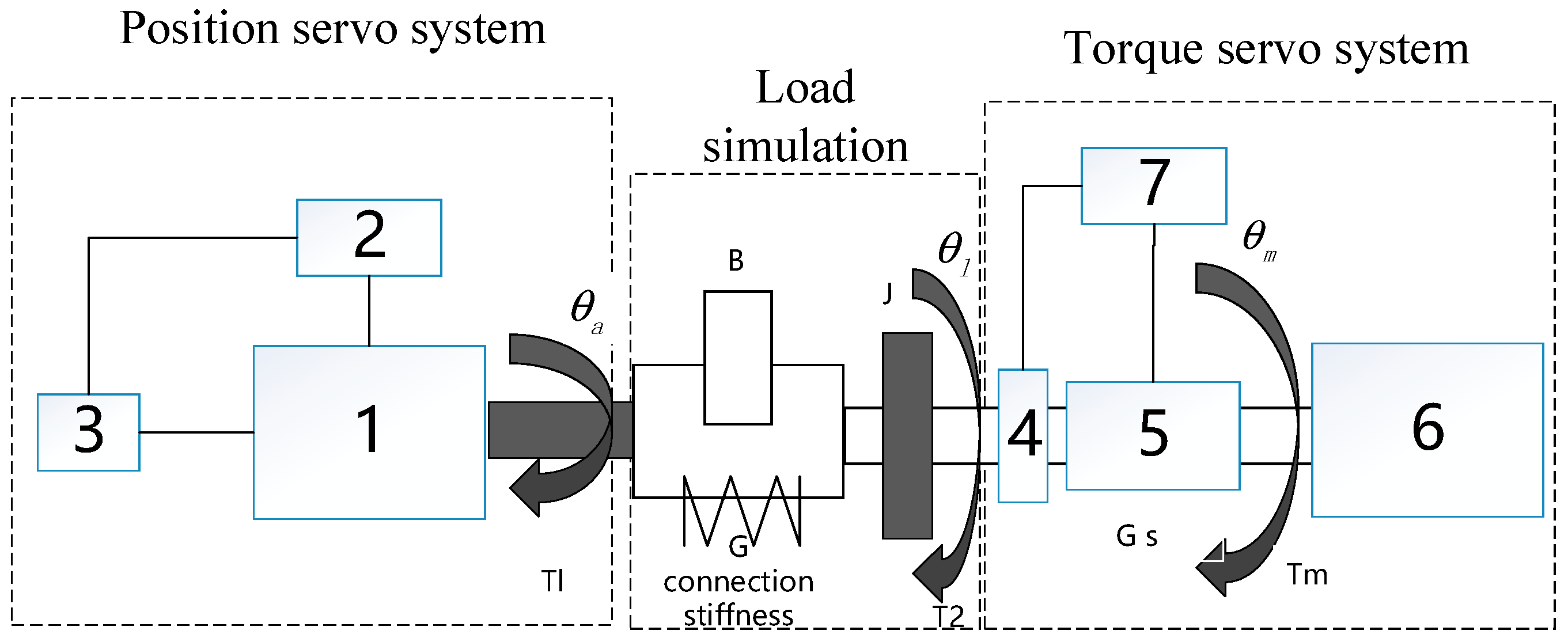
2.1. Introduction of ACS

As is shown in Figure 1, the left part is the position servo system to simulate the angle of the aircraft side-stick, while the right part is the torque servo system which simulates the torque of the active side-stick. In the position servo system, the angle change in motor 1 is collected by the angle displacement sensor 3 and fed back to the controller 2. In the torque servo system, position and torque inputs from the active side-stick, collected by the angle displacement sensor 4 and torque sensor 5, are fed back to the controller 7. Through the load simulation connection, the two systems are coupled with each other.

According to the different input forces of the active side-stick, the controller changes different control modes adaptively. When the thrust applied by the driver to the active side-stick is less than the set starting value, the system is equivalent to a force closed-loop system; when the thrust is greater than the starting value, the system changes from torque control to position control and the position of the active side-stick changes as the pilot continues to increase the thrust; when the set end position is reached, the set load is infinite, the active side-stick cannot be pushed further by the human hand, and the system changes from position control to force control.

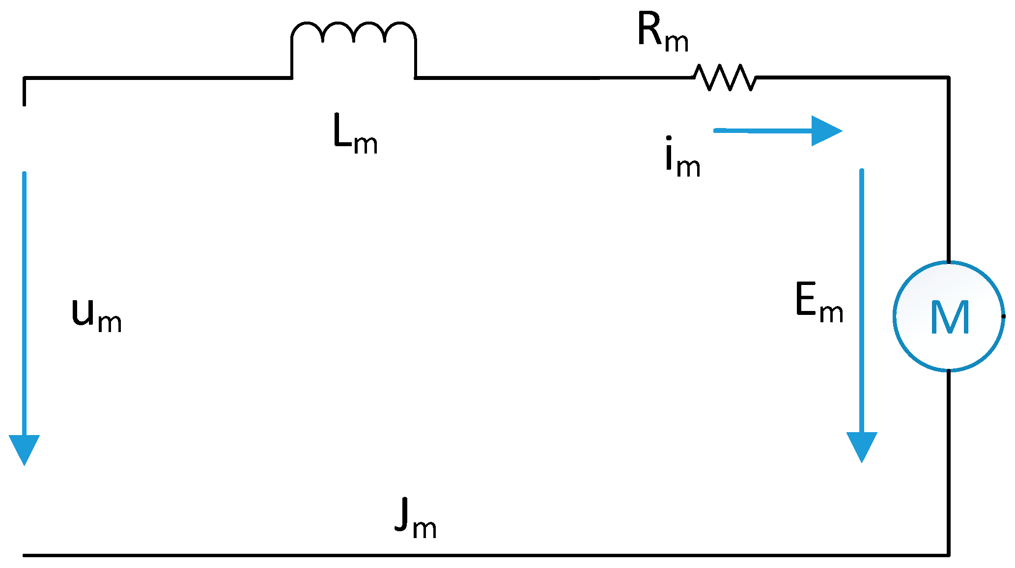
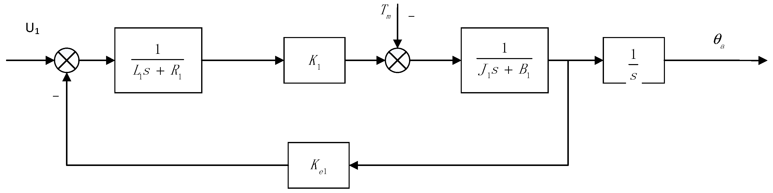
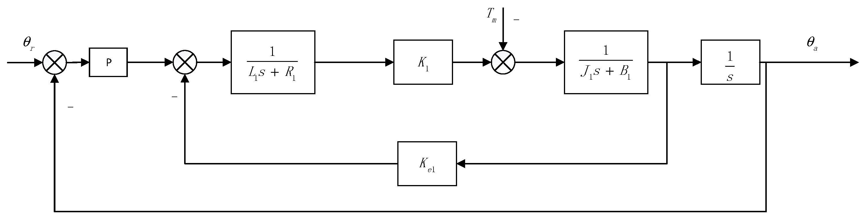
2.2. Modeling of Position Servo System

The model for the power mechanism of the position servo system, with reference to the system principle, is shown in Figure 2 [5,6,7,12]. The equivalent circuit of the motor includes the input voltage, the equivalent loop resistance, the equivalent loop inductance and the back EMF generated by the rotor rotation.

The voltage balance equation of the motor is:

$$u_1=l_1\frac{d{i}_1}{dt}+i_1{r}_1+e_1$$

(1)

At the load end of the equivalent circuit, the back EMF is formed due to the rotation of the motor rotor. The equation of the back EMF is:

$$e_1=K_{e1}\frac{d{\theta }_a}{dt}$$

(2)

As mentioned above, the external disturbance torque received by the position system mainly comes from two parts, one is the friction torque inside the motor, which is represented by the friction force generated by viscous damping, and the other is the load torque applied by the torque system to the position system. The torque balance equation of the motor is then:

$$T_l=J_1\frac{d^2{\theta }_a}{d{t}^2}+B_1\frac{d{\theta }_a}{dt}-T_m$$

(3)

The relationship between the torque and current of the servo torque motor is:

$$T_l=K_1{I}_1\left(s\right)$$

(4)

The Laplace transform of Formulas (1)~(3) can be obtained by:

$$U_1\left(s\right)=L_{1}s{I}_1\left(s\right)+I_1\left(s\right)R_1+E_1\left(s\right)$$

(5)

$$E_1\left(s\right)=K_{e1}s{\theta }_a\left(s\right)$$

(6)

$$T_l\left(s\right)=J_1{s}^2{\theta }_a\left(s\right)+B_{1}s{\theta }_a\left(s\right)-T_m\left(s\right)$$

(7)

Considering the connection stiffness of the motor part to the torque sensor, we can get:

$$T_0\left(s\right)=T_m-G_l({\theta }_l-{\theta }_a)$$

(8)

In the above formula, each variable is defined as:

$U_1$—Input voltage (V);

$L_1$—Equivalent inductance (H);

$I_1$—Circuit current (A);

$R_1$—Equivalent resistance value ($\mathsf{\Omega }$);

$E_1$—Back electromotive force (V);

$K_{\mathrm{e}1}$—Back EMF coefficient ($V·s/rad$);

${\theta }_a$—Equivalent angular displacement of motor output shaft (rad);

${\theta }_l$—Load equivalent angular displacement (rad);

$T_l$—Electromagnetic torque of motor (Nm);

$T_0$—Sum of torques (Nm);

$T_{\mathrm{m}}$—Torque of active side-stick (Nm);

$J_1$—Rotational inertia of motor ($Kg·m^2$);

$B_1$—Damping coefficient of the position servo system ($N·m·s/rad$);

$K_1$—Electromagnetic torque coefficient of motor ($N·m/A$);

$G_l$—Load equivalent torsional stiffness ($N·m/rad$);

The structure diagram of the position servo system can be obtained from the above formula.

As illustrated in Figure 3, the position servo system consists of two parts, namely the forward channel and the disturbance channel. The transfer function of the forward channel from $U_1$ to ${\theta }_a$ is:

$$\frac{{\theta }_a\left(s\right)}{U_1\left(s\right)}={\frac{K_{T1}}{\left[L_1{J}_1{s}^2+\left(L_1{B}_1+R_1{J}_1\right)s+R_1{B}_1+K_{T1}{K}_{e1}\right]s}}_{ }$$

(9)

The disturbance channel is from $T_m\left(s\right)$ to ${\theta }_a$, and the transfer function of this channel is:

$$\frac{{\theta }_a\left(s\right)}{T_m\left(s\right)}={\frac{R_1+L_{1}s}{\left[L_1{J}_1{s}^2+\left(L_1{B}_1+R_1{J}_1\right)s+R_1{B}_1+K_1{K}_{e1}\right]s}}_{ }$$

(10)

The current position system is open-loop. In order to realize the closed-loop control of the position system, assuming the position closed-loop controller is $P\left(s\right)$, the closed-loop control block diagram of the position system is shown in Figure 4:

In the position closed-loop structure diagram, the angular displacement output of the position system consists of two parts:

$${\theta }_a\left(s\right)=A_1\left(s\right){\theta }_r\left(s\right)+B_1\left(s\right)T_m\left(s\right)$$

(11)

where ${\theta }_r$ is the input of interference channel, and $A_1\left(s\right)$ is the transfer function from the angular position instruction to the angular position output:

$$A_1\left(s\right)=\frac{{\theta }_a\left(s\right)}{{\theta }_r\left(s\right)}={\frac{P\left(s\right)K_1}{L_1{J}_1{s}^3+\left(R_1{J}_1+L_1{B}_1\right)s^2+K_{e1}{K}_{1}s+G_c\left(s\right)K_1}}_{ }$$

(12)

where $B_1\left(s\right)$ is the transfer function from the torque input of the torque system to the angular position output of the position system:

$$B_1\left(s\right)=\frac{{\theta }_a\left(s\right)}{T_m\left(s\right)}=\frac{R_1+L_{1}s}{L_1{J}_1{s}^3+\left(R_1{J}_1+L_1{B}_1\right)s^2+K_{e1}{K}_{1}s+P\left(s\right)K_1}$$

(13)

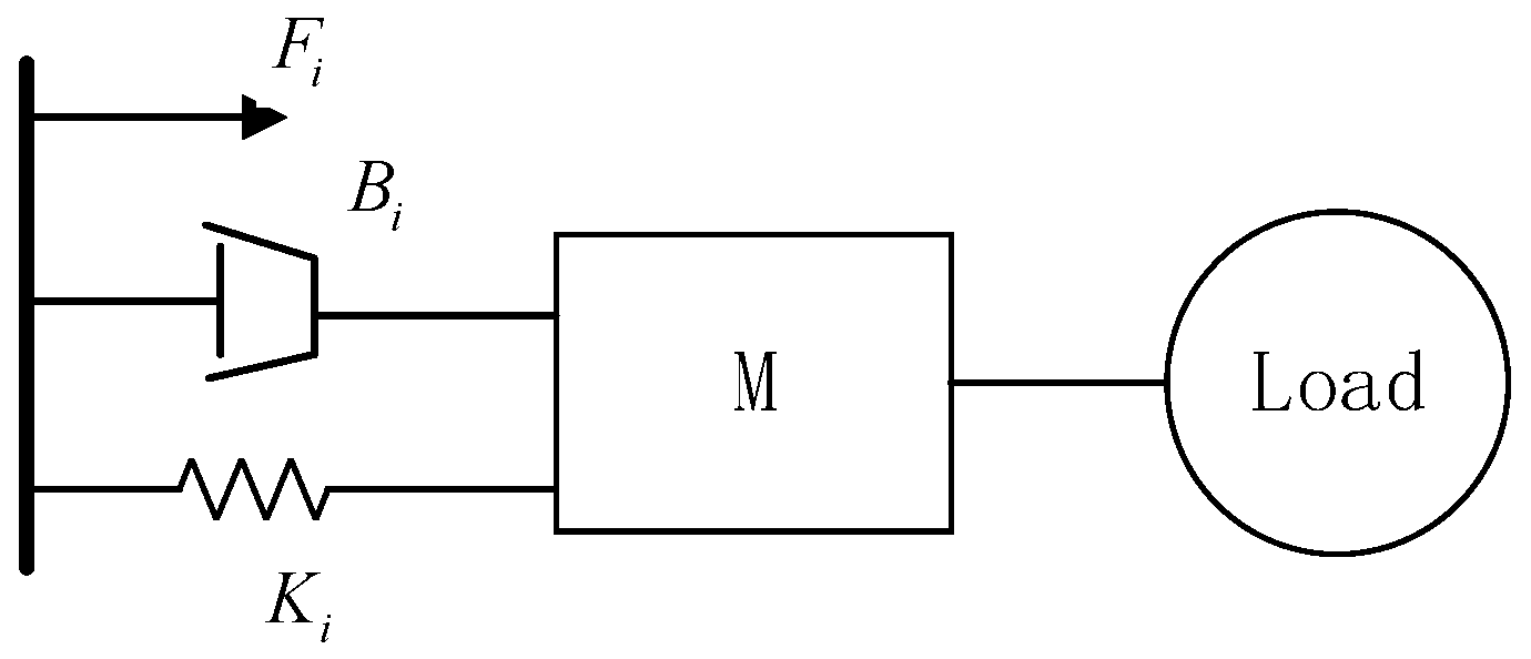
2.3. Modeling of the Artificial Feel System

The principle of the artificial feel system is similar to that of the position servo system. The pilot’s arm muscle system can be regarded as a variable stiffness spring and a variable damping link when manipulating the side-stick. The arm output balance equation is:

$$F=B_x\frac{d\theta }{dt}+K_x\theta$$

(14)

where $K_x$ and $B_x$ are equivalent variable spring stiffness and variable damping, respectively. $K_x$ depends on human tactile information, and can be expressed as $K_x=f\left(\theta ,v\right)$, stiffness and rotation angle, and speed, which is a nonlinear link.

Since springs with a variable stiffness and a variable damping link are nonlinear systems, the arm muscle is simplified as a constant stiffness and constant damping system, and a variable input force is added. The simplified output equation can be obtained from Figure 5 as:

$$F_m=B_i\frac{d{\theta }_m}{dt}+K_i{\theta }_m+F_i$$

(15)

The relationship between output force and torque is:

$$T_2=F_{m}L$$

(16)

According to the precise model of Figure 1, the force balance equation is determined as follows:

$$T_2=J_m^{\prime }\frac{d{\theta }_m^2}{dt}+B_m^{\prime }\frac{d{\theta }_m}{dt}+G_s\left({\theta }_m-{\theta }_l\right)$$

(17)

The load balance equation is listed between the motor output end and the torque sensor:

$$G_s\left({\theta }_m-{\theta }_l\right)=J_l\frac{d^2{\theta }_l}{d{t}^2}+B_l\frac{d{\theta }_l}{dt}+G_l\left({\theta }_l-{\theta }_a\right)$$

(18)

Output torque is:

$$T_m=G_s\left({\theta }_m-{\theta }_l\right)$$

(19)

The Laplace transform of above formulas can be obtained:

$$F_m=B_{i}s{\theta }_m+K_i{\theta }_m+F_i$$

(20)

$$T_2=J_m^{\prime }{s}^2{\theta }_m^2+B_m^{\prime }s{\theta }_m+G_s\left({\theta }_m-{\theta }_l\right)$$

(21)

$$G_s\left({\theta }_m-{\theta }_l\right)=J_l{s}^2{\theta }_l+B_{l}s{\theta }_l+G_l\left({\theta }_l-{\theta }_a\right)$$

(22)

In the above formula, each variable is defined as:

$F_m$—Output force of the artificial feel system (N);

$B_i$—Equivalent damping coefficient of arm muscle ($\mathrm{N}·\mathrm{m}·\mathrm{s}/\mathrm{rad}$);

$K_i$—Equivalent spring stiffness of arm muscle (N/m);

$F_i$—Variable force of arm output (N);

$T_2$—Output torque (Nm);

$G_{\mathrm{s}}$—Torsional stiffness of torque sensor (N/rad);

${\theta }_m$—Output angular displacement of active side-stick (rad);

$J_l$—Inertia of equivalent load ($\mathrm{Kg}·{\mathrm{m}}^2$);

$B_l$—Damping coefficient of equivalent load ($\mathrm{N}·\mathrm{m}·\mathrm{s}/\mathrm{rad}$);

$L$—Effective length of side-stick (m);

$B_m^{\prime }$—Equivalent damping coefficient of torque system ($\mathrm{N}·\mathrm{m}·\mathrm{s}/\mathrm{rad}$);

$J_m^{\prime }$—Equivalent moment of inertia of torque system ($\mathrm{Kg}·{\mathrm{m}}^2$);

The upper $F_i$ relates to human tactile information (including angle and speed). According to the above equation, the block diagram of the artificial feel system can be obtained in Figure 6.

The transfer function of output torque is expressed as follows:

$$T_m\left(s\right)=A_3\left(s\right)F_i\left(s\right)+B_3\left(s\right){\theta }_m\left(s\right)$$

(23)

$$A_3\left(s\right)=\frac{L{G}_s\left(J_l{s}^2+B_{l}s+G_l\right)}{D_2\left(s\right)}$$

(24)

$$B_3\left(s\right)=\frac{G_l\left(-J_m^{\prime }{s}^2+(L{B}_i-B_m^{\prime }\right)s+L{K}_i)}{D_2\left(s\right)}$$

(25)

$$D_2\left(s\right)=J_m^{\prime }{J}_l{s}^4+(J_m^{\prime }{B}_l+B_m^{\prime }{J}_l-L{J}_l{B}_i)s^3+\left(J_m^{\prime }{G}_s+B_m^{\prime }{B}_l+J_m^{\prime }{G}_l+J_l{G}_s-L{K}_i{J}_l-L{B}_i{B}_l\right)s^2+\left(B_m^{\prime }{G}_l+B_m^{\prime }{G}_s+G_s{B}_l-L{G}_s{B}_i-L{K}_i{B}_i-L{G}_l{B}_i\right)s+G_s{G}_l-L{G}_s{K}_i-L{K}_i{G}_l$$

(26)

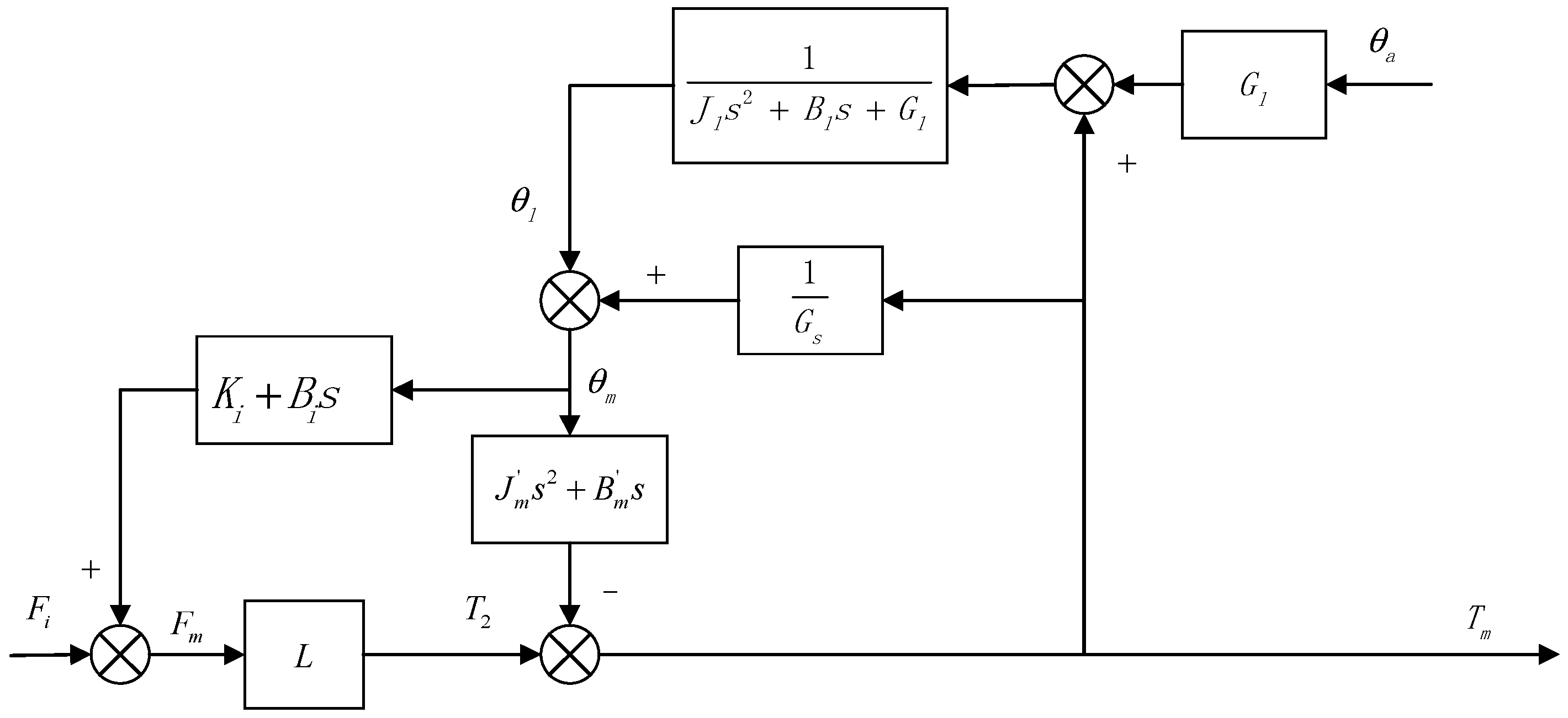
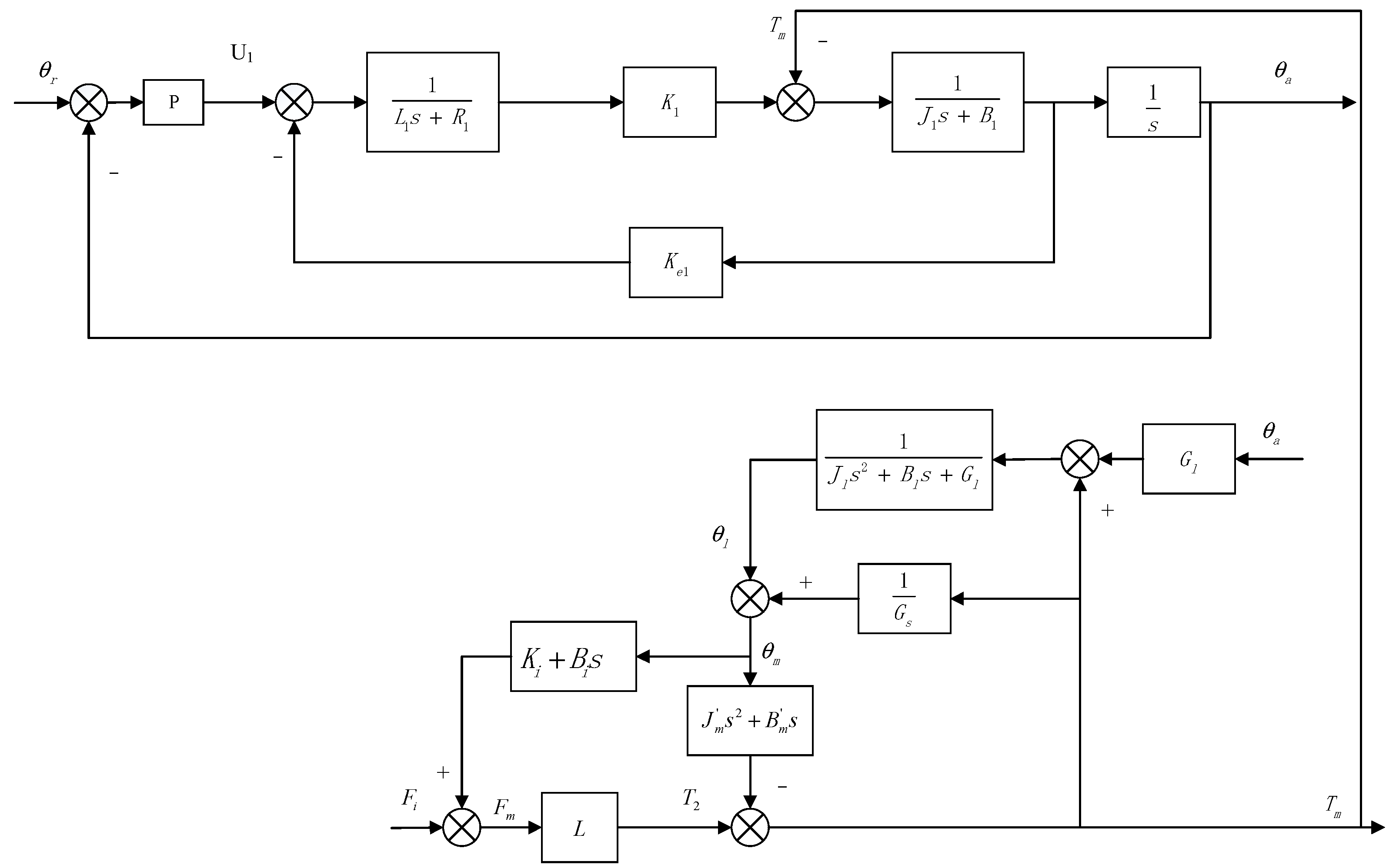
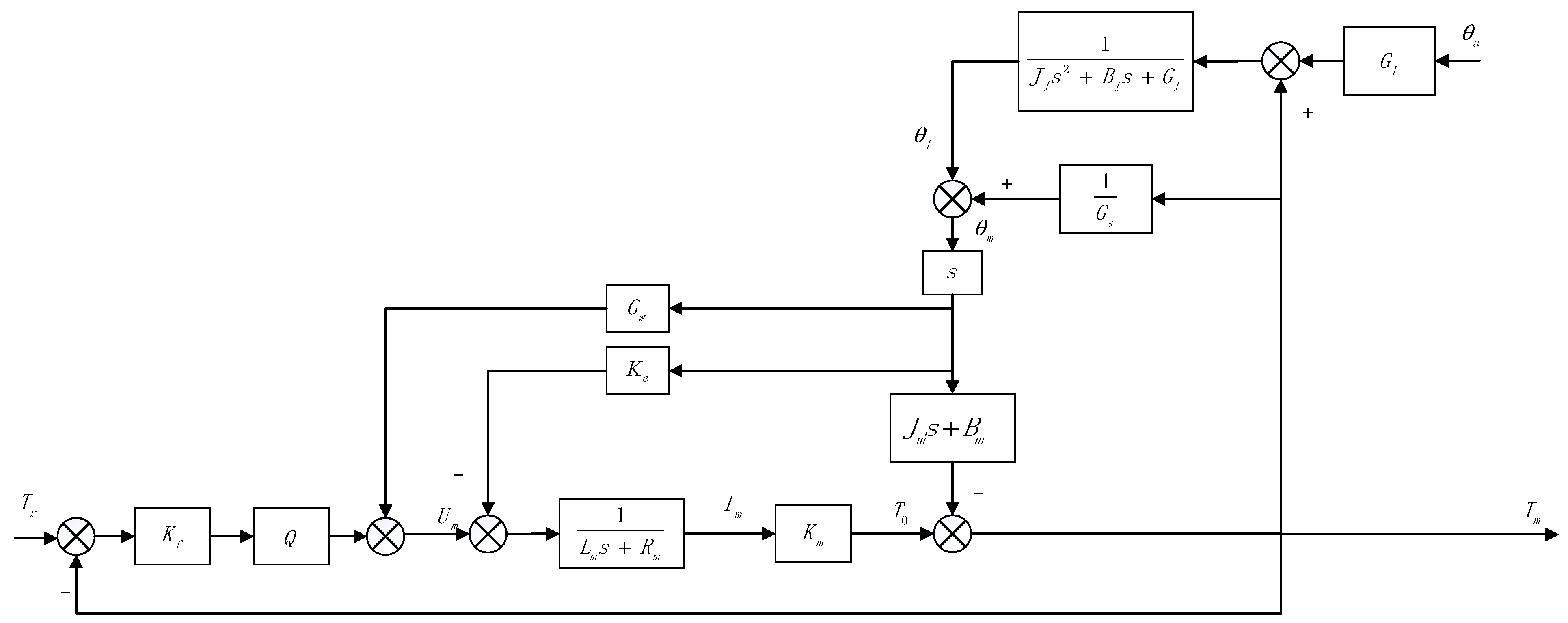
2.4. Modeling of Coupling System

When the mathematical model of the artificial feel system is combined with the position system, the coupling mathematical model can be obtained, as shown in Figure 7.

Considering disturbance inputs, the force instruction $F_i$ is the input of forward channel, ${\theta }_r$ is the input of the interference channel, and $T_m$ is the output; the transfer function can be obtained as follows:

$$T_m\left(s\right)=\frac{A_3\left(s\right)}{1-B_3\left(s\right)B_1\left(s\right)}{F}_i\left(s\right)+\frac{B_3\left(s\right)A_1\left(s\right)}{1-B_3\left(s\right)B_1(s)}{\theta }_r\left(s\right)$$

(27)

According to the system transfer function, when $F_i$ is zero, the value of ${\theta }_r$ fluctuates, $T_m$ represents surplus torque, and output torque is affected by the position system. This is one of the problems we need to solve, namely, the accuracy of the system. Secondly, for the servo system, we should improve its tracking performance, namely rapidity.

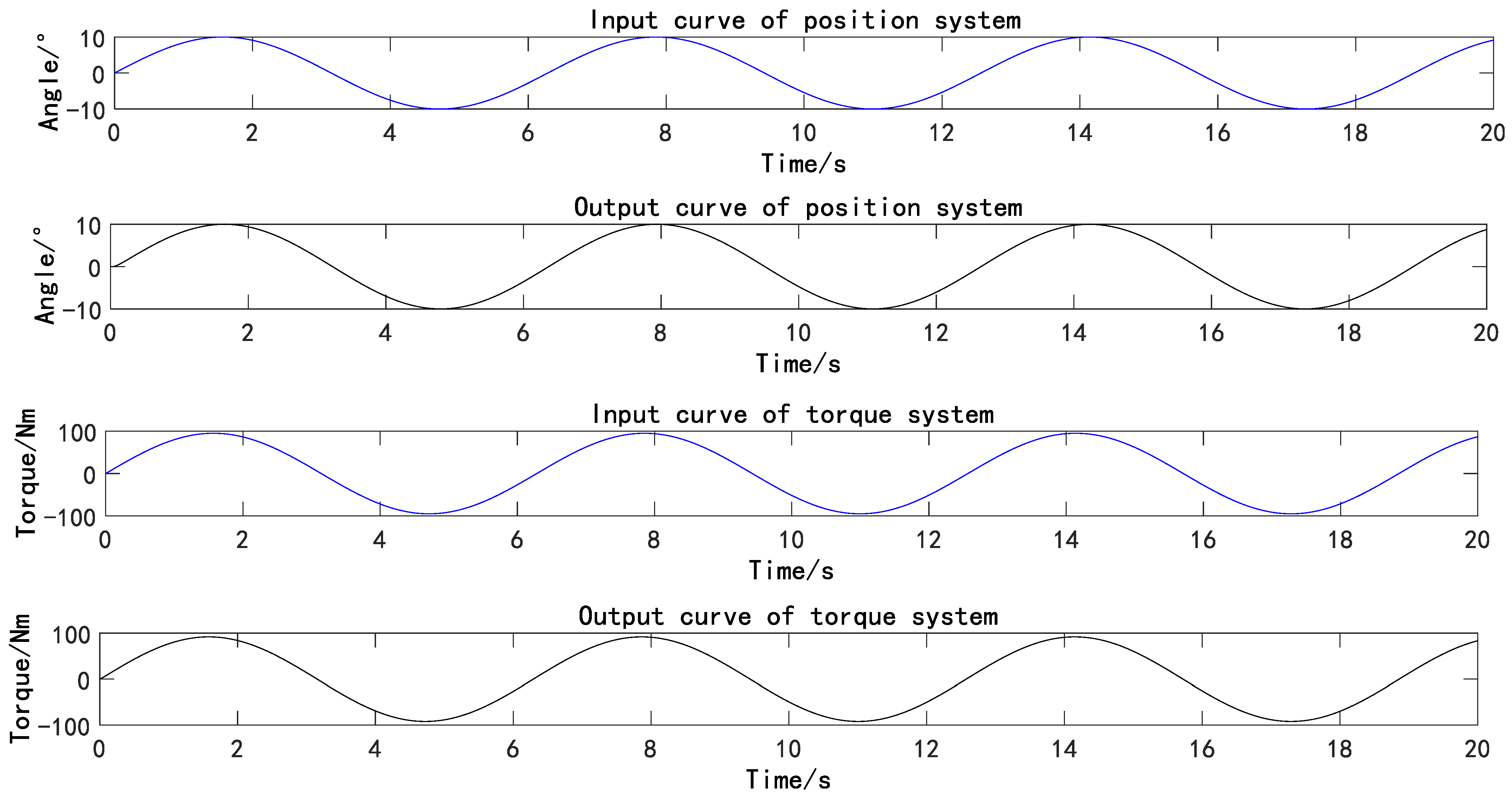
3. Servo Characteristics Analysis

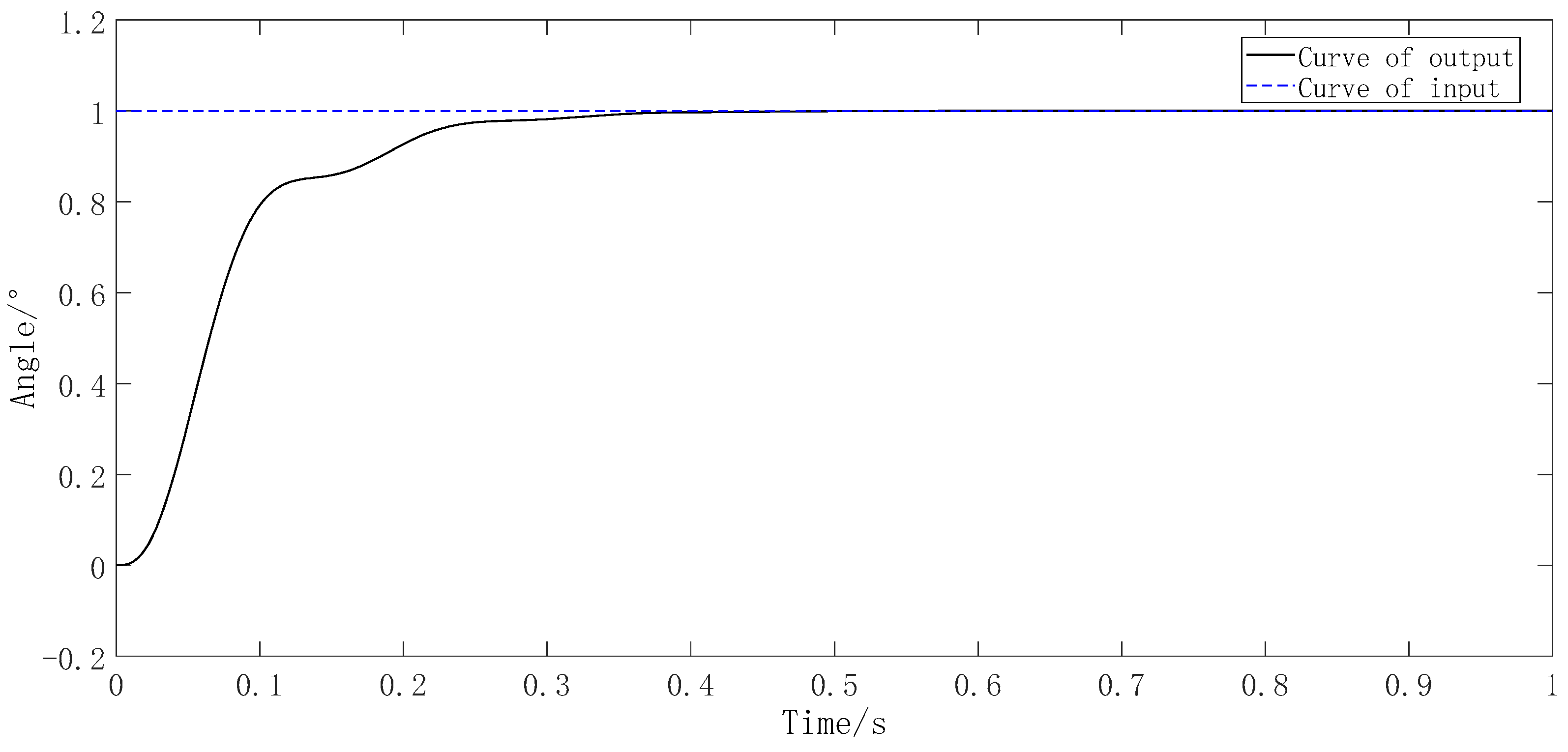
3.1. Simulation and Analyze

Through the selection of the DC servo motor, torque motor, coupling and torque sensor, the values of each system parameter is preliminarily determined.

According to a project, a position closed-loop controller $P\left(s\right)$ is as follows:

$$P\left(s\right)=12+0.012\frac{1}{s}$$

(28)

The unit step response of the system is then as follows:

It can be seen from Figure 8 that the step response performance index of the position system is: Response process without overshoot; adjust time 0.28 s (take 5% error band); no steady-state error.

The sine angle instruction with an amplitude of $1^{°}$ and a frequency of $67.23 \mathrm{rad}/\mathrm{s}$ is given to the position system. Taking the time range of 0~2 s, the comparison between the instruction curve and the tracking curve is shown in Figure 9.

It can be seen that the tracking curve in the above figure lags behind the instruction curve by 0.011 s, and the amplitude of the tracking curve is 0.707 times that of the instruction, indicating that the system bandwidth is about 10.7 Hz.

Next, we studied the coupling of the two systems. The input amplitude of the position system is the command with frequency; the torque command with an amplitude of 100 N and a frequency of 1 rad/s, as given by the torque system. When the two systems are not coupled, the input and output curves of the two systems are shown in Figure 10.

For two sets of system inputs with the same instruction, and with the respective output as a disturbance input to the other system forming a coupling effect, the input and output contrast curve is shown in Figure 11.

It can be seen that when the two systems are coupled together, compared with Figure 12, the sinusoidal output amplitude of the position system decreases slightly, and the amplitude is about 9, while the output of the torque system increases, and the amplitude is about 105. The output of the two systems has changed because they have strong disturbances entering the system which affect the output of the system. It is worth noting that the sinusoidal output of the torque system has a sawtooth jitter, which may be caused by the interference torque of the torque system. In the next section we discuss this phenomenon and eliminate this jitter.

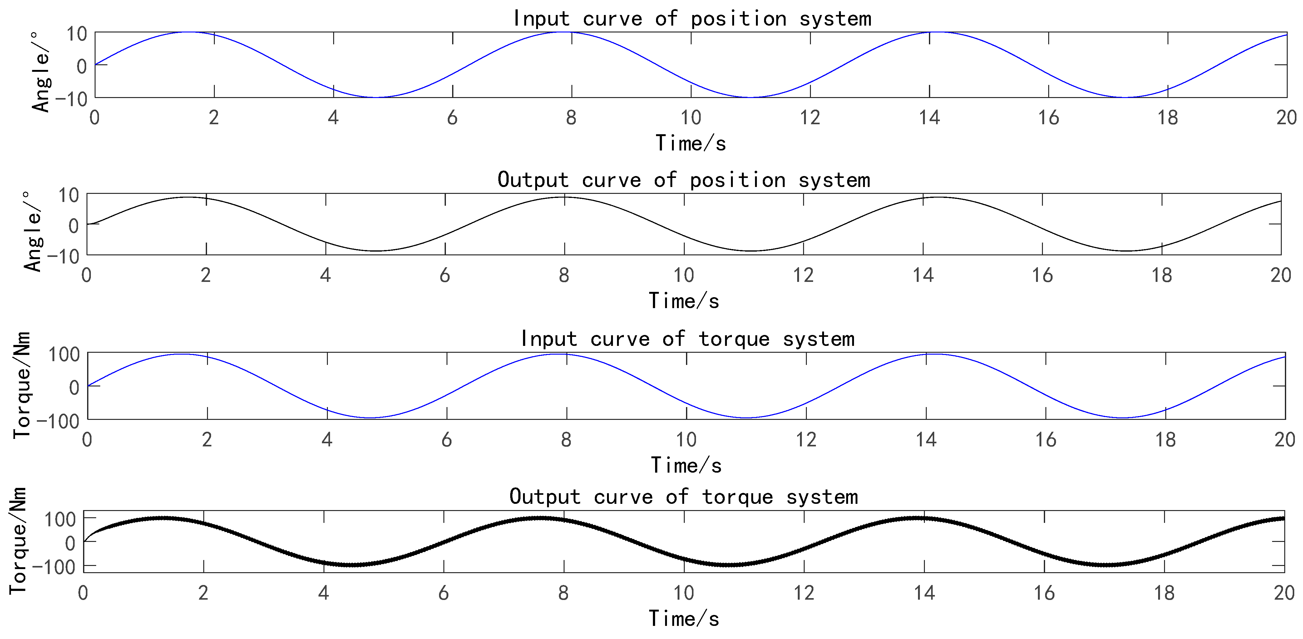
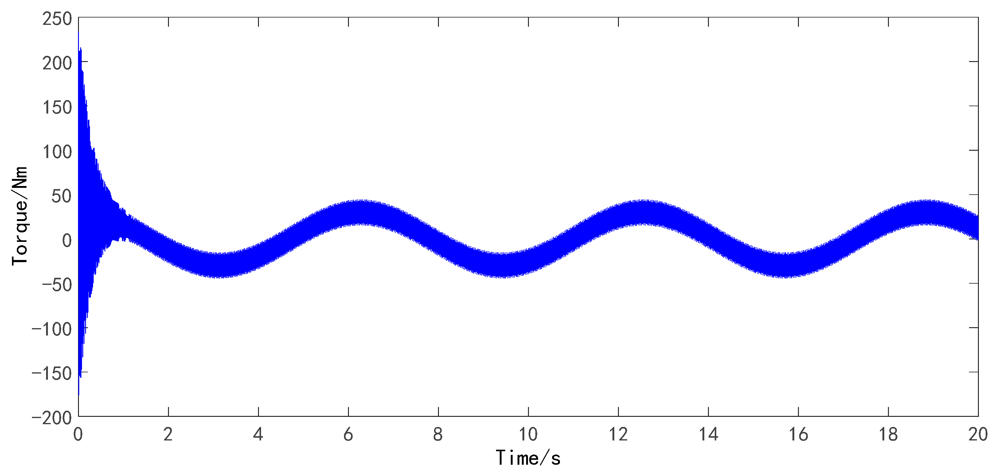
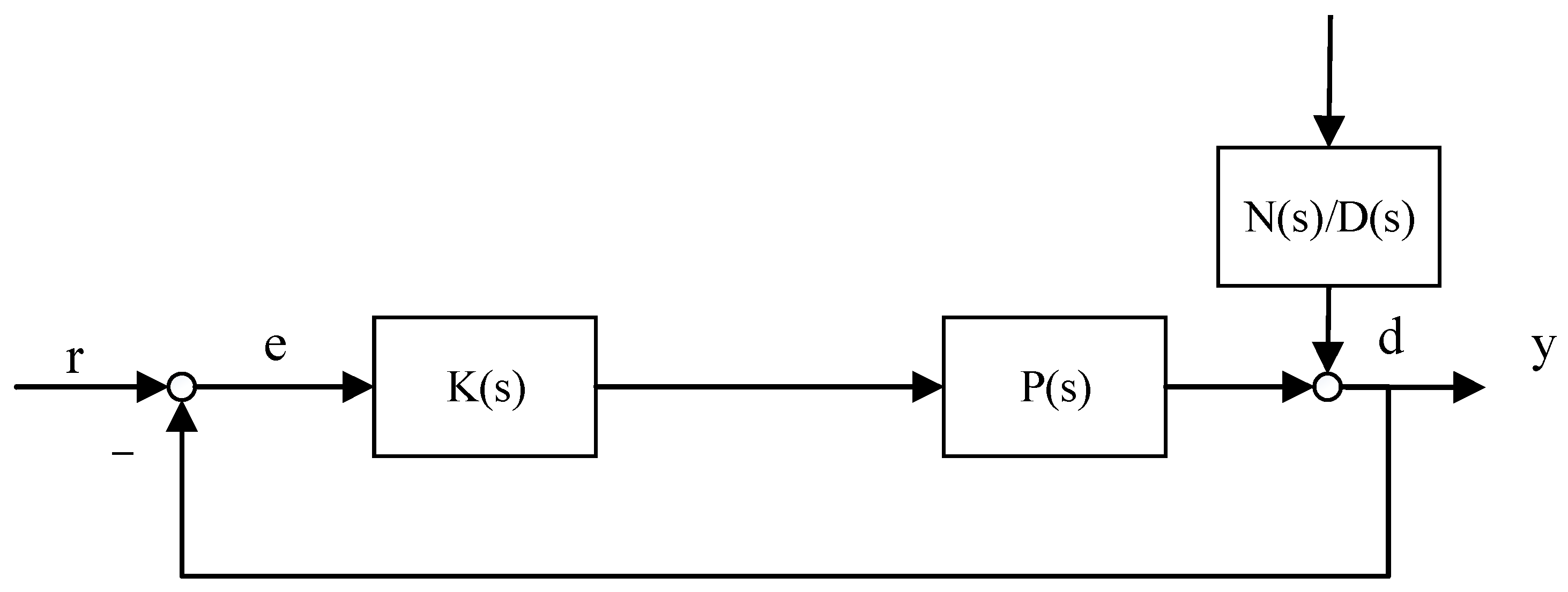
3.2. Interference Torque Suppression Based on Dynamic Compensation

There are two main ways to suppress interference torque: hardware compensation or software compensation. The dynamic compensation method based on the principle of structural invariance is a software compensation method [12,17]. In order to offset the interference of an external angle input, the principle of designing a dynamic compensation controller based on state observation is as follows:

$w$ is the disturbance signal and $G_3$ is the influence of external disturbance on the system. The appropriate $G_b\left(s\right)$ is designed to suppress the disturbance, and the compensation link needs to meet: $G_b=\frac{G_3}{G_1}$.

The angular velocity dynamic compensation link is set to $G_{\omega }\left(s\right)$, and the control system structure diagram with dynamic compensation is shown in Figure 13:

According to the formula $G_b=\frac{G_3}{G_1}$ of the previous design principle, two channels need to be calculated for dynamic compensation. The compensation link can be calculated by the superposition principle as follows:

$$G_{\omega }\left(s\right)=\frac{L_m{J}_m{s}^2+\left(R_m{J}_m+L_m{B}_m\right)s+L_m{B}_m}{K_t}$$

(29)

The sinusoidal signal with a frequency of 1 rad/s and an amplitude of 10° is manually inputted on the disturbance channel, and the output curve of the torque system is shown in Figure 14.

However, by observing the feedforward compensation link, it is difficult to achieve better quality. On the one hand, the high-order pure differential link will introduce interference into the system to make the control effect worse; on the other hand, the differential in the computer control system is realized in a differential way. A higher-order differential is bound to slow down the overall control speed of the system and make the system quality worse. Therefore, in specific applications, low-pass filters are usually added to the compensation link to filter high-frequency interference and to make it easier to implement. The compensation link after filtering is added is as follows:

$$G_{\omega }\left(s\right)=\frac{L_m{J}_m{s}^2+\left(R_m{J}_m+L_m{B}_m\right)s+R_m{B}_m}{K_t{(\tau s+1)}^2}$$

(30)

The output curve of the system with a low-pass filter is as shown in Figure 15:

It can be seen that the compensated signal has less high-frequency interference when the filter is added. At this time, the coupling system with dynamic compensation is simulated, as shown in Figure 16.

Compared with the coupling system before and after dynamic compensation, it can be seen that the output curve of the torque system after compensation is smoother, the system quality is greatly improved, and the vibration and interference can basically be eliminated.

3.3. System Simulation and Analysis

In order to detect the frequency response characteristics of the system in the middle and low frequency ranges, the position system is set to a 0.1–20 frequency sweep. When the starting state time is zero, the command frequency is 0.1, and the command frequency is gradually increased to 20 in the thirtieth second. The command and simulation comparison curves are shown in Figure 17.

From the above simulation frequency response tracking curve, it can be seen that when the torque system is in the low frequency range of 0.1–15, the simulation curve tracking command curve is good, with no lag phenomenon; basically no amplitude attenuation phenomenon. When the system is between 16 and 20, the actual simulation curve shows amplitude attenuation, which is about 70.7% of the command curve, and there is no phase lag in the middle frequency band. By calculating the system bandwidth of about 16, this phenomenon is also explained from the side. In order to better-test the frequency response characteristics of the system, we carried out the sweep frequency tracking curve in time domain (fast Fourier transform), and the results are shown in Figure 18.

The comparison between the instructions and the actual curve can be seen in Figure 18. After transforming the frequency response tracking curve in Figure 18 into frequency domain, it is easier to see that the actual working curve is between 16 and 20 Hz, and there is a characteristic of amplitude attenuation. There is no phase lag or advance in the sweep process. In general, the system demonstrates good tracking at low frequencies.

4. Robust Controller Design

4.1. System State-Space Equations

The main content of robustness analysis of control systems analyzes the stability, steady-state performance and dynamic characteristics of control systems under a set of uncertainties.

As is illustrated in Figure 19, standard $H_{\infty }$ control problem: for the above closed-loop control system, all real rational controllers K are found to make the closed-loop control system internally stable, and the $H_{\infty }$ norm of the closed-loop transfer function matrix $T_{zw}$ is effective at a given constant γ > 0, namely [21,22,23,24,25,26]:

$$|\left|F_l\left(G,K\right)\right|{|}_{\infty }<\gamma$$

(31)

For the active side-stick control system studied in this paper, we focused on the torque system, and the output of the position system is applied to the disturbance channel. According to the differential equation of the system, we selected the state variables $x_1=i$, $x_2={\theta }_m$, $x_3=\dot{{\theta }_m}$, $x_4={\theta }_l$, $x_5=\dot{{\theta }_l}$, where $w={\theta }_a$ is the external input, and where the speed of the driving side-stick is represented as the disturbance of the position system; z is the controlled output; the system output $y=T_m$, representing the measured output of the system, is the torque output of the position system. As the control input of the system, $u=T_f$ represents the torque command input into the control system. Thus, the following equations can be obtained:

$${\dot{x}}_1=-\frac{R_m}{L_m}{x}_1-\frac{K_f{G}_s}{L_m}{x}_2-\frac{K_e}{L_m}{x}_3+\frac{K_f{G}_s}{L_m}{x}_4+\frac{K_f}{L_m}{T}_f$$

(32)

$${\dot{x}}_2=x_3$$

(33)

$${\dot{x}}_3=\frac{K_m}{J_m}{x}_1-\frac{G_s}{J_m}{x}_2-\frac{B_m}{J_m}{x}_3+\frac{G_s}{J_m}{x}_4$$

(34)

$${\dot{x}}_4=x_5$$

(35)

$${\dot{x}}_5=\frac{G_s}{J_l}{x}_2-\frac{G_s+G_l}{J_l}{x}_4-\frac{B_l}{J_l}{x}_5+\frac{G_l}{J_l}{\theta }_a$$

(36)

$$y=G_s{x}_2-G_s{x}_4$$

(37)

The system state equation can be obtained from the above equations:

$$\left[\begin{array}{c}{\dot{x}}_1\\ {\dot{x}}_2\\ {\dot{x}}_3\\ {\dot{x}}_4\\ {\dot{x}}_5\end{array}\right]=\left[\begin{array}{ccccc}-\frac{R_m}{L_m}& -\frac{K_f{G}_s}{L_m}& -\frac{K_e}{L_m}& \frac{K_f{G}_s}{L_m}& 0\\ 0& 0& 1& 0& 0\\ \frac{K_m}{J_m}& -\frac{G_s}{J_m}& -\frac{B_m}{J_m}& \frac{G_s}{J_m}& 0\\ 0& 0& 0& 0& 1\\ 0& \frac{G_s}{J_l}& 0& -\frac{G_s+G_l}{J_l}& -\frac{B_l}{J_l}\end{array}\right]\left[\begin{array}{c}{x}_1\\ x_2\\ x_3\\ x_4\\ x_5\end{array}\right]+\left[\begin{array}{c}\frac{K_f}{L_m}\\ 0\\ 0\\ 0\\ 0\end{array}\right]+T_f+\left[\begin{array}{c}0\\ 0\\ 0\\ 0\\ \frac{G_l}{J_l}\end{array}\right]{\theta }_a$$

(38)

$$\mathrm{y}=G_s\left[\begin{array}{ccccc}0& 1& 0& -1& 0\end{array}\right]\left[\begin{array}{c}{x}_1\\ x_2\\ x_3\\ x_4\\ x_5\end{array}\right]$$

(39)

The data of

Table 1. System parameters.

Variable	Value	Unit
${\mathrm{J}}_1$	0.0689	$\mathrm{Kg}·{\mathrm{m}}^2$
${\mathrm{J}}_{\mathrm{l}}$	0.0495	$\mathrm{Kg}·{\mathrm{m}}^2$
${\mathrm{L}}_1$	0.0297	H
${\mathrm{R}}_1$	2.36	$\mathsf{\Omega }$
${\mathrm{B}}_1$	0.39	$\mathrm{N}·\mathrm{m}·\mathrm{s}/\mathrm{rad}$
${\mathrm{B}}_{\mathrm{l}}$	0.34	$\mathrm{N}·\mathrm{m}·\mathrm{s}/\mathrm{rad}$
${\mathrm{K}}_{\mathrm{e}1}$	1.258	$\mathrm{V}·\mathrm{s}/\mathrm{rad}$
${\mathrm{K}}_1$	7.9	$\mathrm{N}·\mathrm{m}/\mathrm{A}$
${\mathrm{G}}_{\mathrm{s}}$	10,585	$\mathrm{N}·\mathrm{m}/\mathrm{rad}$
${\mathrm{G}}_{\mathrm{l}}$	11,421	$\mathrm{N}·\mathrm{m}/\mathrm{rad}$
${\mathrm{B}}_{\mathrm{i}}$	0.41	$\mathrm{N}·\mathrm{m}·\mathrm{s}/\mathrm{rad}$
${\mathrm{K}}_{\mathrm{i}}$	25	N/m
$\mathrm{L}$	0.5	m
${\mathrm{B}}_{\mathrm{m}}^{\prime }$	0.16	$\mathrm{N}·\mathrm{m}·\mathrm{s}/\mathrm{rad}$
${\mathrm{J}}_{\mathrm{m}}^{\prime }$	0.0135	$\mathrm{Kg}·{\mathrm{m}}^2$

are substituted into the calculation to obtain:

$$A=\left[\begin{array}{ccccc}-95.24& -95.24& -28.57& 95.24& 0\\ 0& 0& 1& 0& 0\\ 170.37& -211500& -4.26& 211500& 0\\ 0& 0& 0& 0& 1\\ 0& 122149.73& 0& -213903.74& -4.81\end{array}\right]$$

(40)

$$B=\left[\begin{array}{cc}0.0083& 0\\ 0& 0\\ 0& 0\\ 0& 0\\ 0& 106951.9\end{array}\right]$$

(41)

$$C=\left[\begin{array}{ccccc}0& 1& 0& -1& 0\end{array}\right]$$

(42)

Simplified as follows:

$$\left\{\begin{array}{c}{\dot{x}}_1=AX+B_1{T}_f+B_2{\theta }_a\\ Y=CX\end{array}\right.$$

(43)

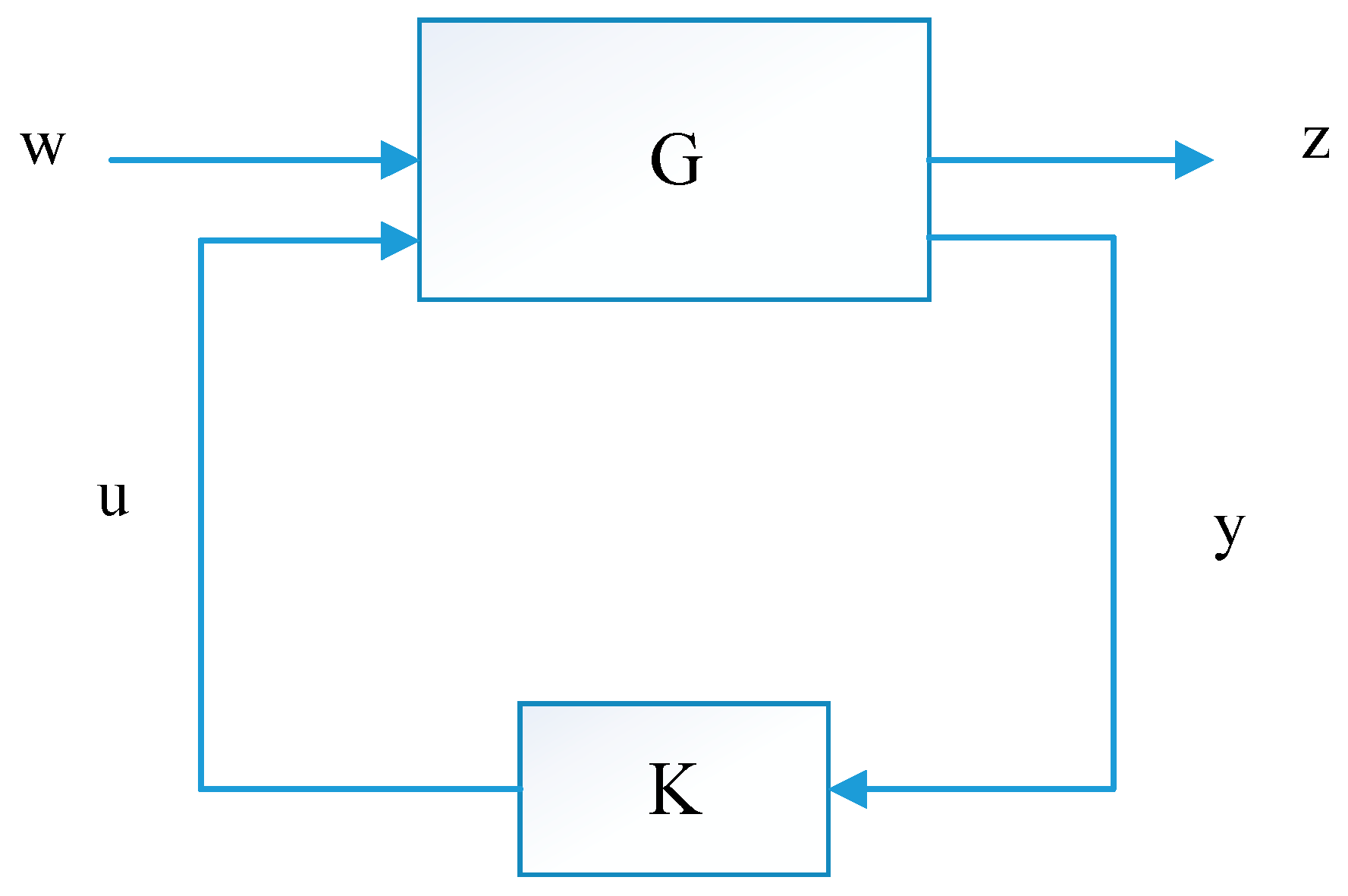
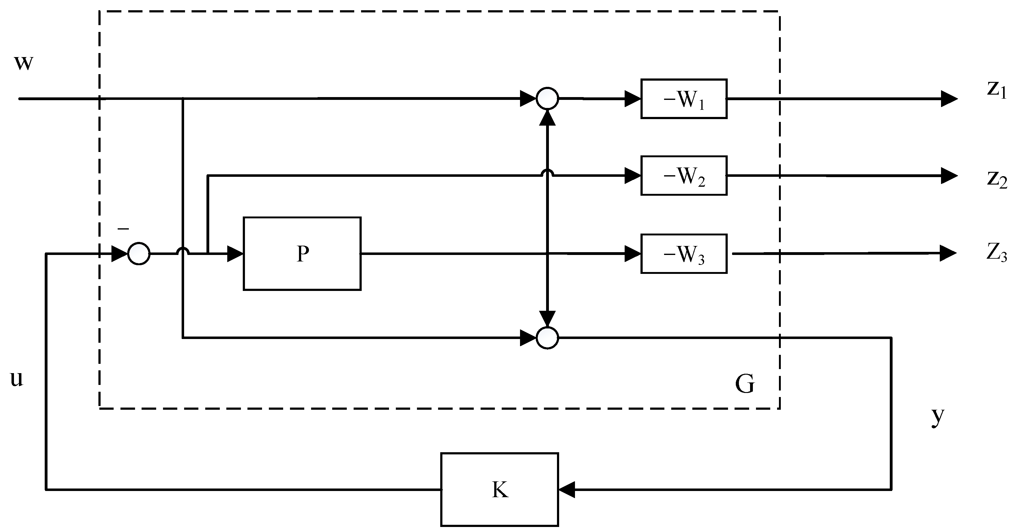
4.2. Mixed Sensitivity Control Problem

In this paper, in order to promote the stability of design under uncertainty, a mixed sensitivity method is proposed to evaluate not only the system performance, but also its sensitivity to design parameters. A comprehensive controller design is proposed to improve the robustness of parameter uncertainty. This method uses the trajectory sensitivity to model the parameter uncertainty, and introduces the complementary sensitivity function to reduce the parameter sensitivity of the input and output of the equipment.

The mixed sensitivity control problem follows the following equations:

$$S\left(s\right)={\left[I+P\left(s\right)K\left(s\right)\right]}^{-1}$$

(44)

$$T\left(s\right)={\left[I+P\left(s\right)K\left(s\right)\right]}^{-1}P\left(s\right)K\left(s\right)$$

(45)

$$S\left(s\right)+T\left(s\right)=I$$

(46)

$$min{\left|\left|S\left(s\right)\right|\right|}_{\infty }$$

(47)

In this paper, in order to suppress the influence of $\omega$, namely the speed of the driving side-stick, on the output force of the system, it is hoped that the smaller $S$ is the better. The existence of uncertainties, such as unmodeled dynamics, friction and noise is expected to be as small as $\mathrm{T}$, which is obviously contradictory. S(s) and T(s) must be separated from the small frequency domain. The above indicators can be equivalently described as:

$${\left|\left|S\left(j\omega \right)\right|\right|}_{\infty }<{\epsilon }_1, \left(\omega \in {\mathsf{\Omega }}_1\right)$$

(48)

$${\left|\left|T\left(j\omega \right)\right|\right|}_{\infty }<{\epsilon }_2, \left(\omega \in {\mathsf{\Omega }}_2\right)$$

(49)

where ${\mathsf{\Omega }}_1$ is low frequency and ${\mathsf{\Omega }}_2$ is high frequency. Due to the characteristics of this regional division, it is necessary to start from the following:

$$\sup \left[{\left|\left|W_1\left(j\omega \right)S\left(j\omega \right)\right|\right|}^2+{\left|\left|W_2\left(j\omega \right)T\left(j\omega \right)\right|\right|}^2\right]<{\mathsf{\gamma }}^2$$

(50)

The above conditions are equivalent:

$${||\left[\begin{array}{c}{W}_{1}S\\ W_{2}T\end{array}\right]||}_{\infty }<\gamma$$

(51)

As shown in the figure, according to the formula for the foreshadowing, we can know that the generalized control object at this time is shown in Figure 20.

$$G=\left[\begin{array}{cc}{G}_{11}& G_{12}\\ G_{21}& G_{22}\end{array}\right]=\left[\begin{array}{cc}{W}_1& -W_{1}P\\ 0& W_{2}P\\ 0& W_{3}P\\ I& -P\end{array}\right]$$

(52)

Among them, $G_{11}=\left[\begin{array}{c}{W}_1\\ 0\\ 0\end{array}\right]$, $G_{12}=\left[\begin{array}{c}-W_{1}P\\ W_{2}P\\ W_{3}P\end{array}\right]$, $G_{21}=I$, $G_{22}=-P$ The mixed sensitivity control problem is to find the controller K, stabilize the G described by the above formula and make the linear fractional transformation $\left|\right|F_l\left(G,K\right)|{|}_{\infty }<\gamma$ hold.

The control objective of the active side-stick control system in this paper is to add the voltage variation u to the torque motor. According to the state equation obtained before, the transfer function of the system can be obtained as follows:

$$P\left(s\right)=C{\left(sI-A\right)}^{-1}B=\frac{K_m{G}_s\left(J_l{s}^2+B_{l}s+G_l\right)}{D_0\left(s\right)}$$

(53)

As is shown in Figure 21, K(s) is the controller. The open-loop transfer function is:

$$L\left(s\right)=P\left(s\right)K\left(s\right)$$

(54)

Sensitivity function S(s) and complementary sensitivity function T(s) are:

$$S\left(s\right)={\left[1+L\left(s\right)\right]}^{-1}$$

(55)

$$T\left(s\right)=L\left(s\right){\left[1+L\left(s\right)\right]}^{-1}$$

(56)

In summary, the requirements can be summarized as follows:

$${\left|\left|W_1\left(s\right)S\left(s\right)\right|\right|}_{\infty }<1$$

(57)

In the above expression, $W_1\left(s\right)$ is a stable rational scalar function.

The transfer function P(s), as a design simulation, has uncertainty which cannot be avoided. The reasons for the uncertainty mainly come from the neglected nonlinear factors, unmodeled dynamic characteristics and parameter errors. Here, the uncertain control object $\tilde{P}\left(s\right)$ is expressed as a system with multiplicative uncertainty:

$$\tilde{P}\left(s\right)=[1+W_3\left(s\right)\Delta \left(s\right)]P\left(s\right)$$

(58)

$W_3\left(s\right)$ is the scalar frequency weighting function of multiplicative uncertainty, $\Delta \left(s\right)$ is stable and satisfies $\left|\left|\Delta \left(s\right)\right|\right|<1$. If the closed-loop control system at $\Delta \left(s\right)=0$ is stable, and for P(s), expressed by the above equation, the condition for controller K(s) to stabilize the closed-loop control system is:

$${\left|\left|W_3\left(s\right)T\left(s\right)\right|\right|}_{\infty }<1$$

(59)

Generally, the selected $W_1\left(s\right)$ has a large gain in the low frequency range, while the selected $W_3\left(s\right)$ has a large gain in the high frequency range. $W_2\left(s\right)$ represents set system performance requirements, $R\left(s\right)=K\left(s\right){\left[1+L\left(s\right)\right]}^{-1}$,

According to the maximum singular value property for two matrices A and B:

$$\frac{1}{\sqrt{2}}{\sigma }_{max}\left[\begin{array}{c}A\\ B\end{array}\right]\le max\left\{{\sigma }_{max}\left(A\right), {\sigma }_{max}\left(B\right)\right\}\le {\sigma }_{max}\left[\begin{array}{c}A\\ B\end{array}\right]$$

(60)

Therefore, in summary:

$${||\begin{array}{c}{W}_1\left(s\right)S\left(s\right)\\ W_2\left(s\right)R\left(s\right)\\ W_3\left(s\right)T\left(s\right)\end{array}||}_{\infty }<1$$

(61)

This makes the loading part control problem of the active side-stick control system become a mixed sensitivity control problem.

The above means that in the control block diagram shown in Figure 20, the effect of external input w on the control outputs $z_1$ and $z_2$ is small. In this way, the control problem of the artificial feel system becomes how to find the closed-loop control system which is internally stable and satisfies the controller K above.

G(s) can be obtained.

$$G\left(s\right)=\left[\begin{array}{cc}{W}_1& -W_{1}P\\ 0& W_{2}P\\ 0& W_{3}P\\ I& -P\end{array}\right]$$

(62)

Therefore, the control problem of the active side-stick control system is to find a robust controller K, so that the closed-loop control system shown in Figure 20 is internally stable. According to the following formula:

$$\left|\right|F_l\left(G,K\right)|{|}_{\infty }<1$$

(63)

This is a standard $H_{\infty }$ control problem, and the controller K can be obtained by solving the equation.

4.3. $H_{\infty }$ Controller Design

Firstly, the weighted function $W_1\left(s\right)$ of the sensitivity function S(s) is set as the one-level rational function.

$$W_1\left(s\right)={\mathsf{\gamma }}_1\widetilde{W_1}\left(s\right)$$

(64)

${\gamma }_1$ is a design parameter for adjusting $W_1\left(s\right)$ gain. The greater the value of ${\gamma }_1$, the better the control performance.

$$\widetilde{W_1}\left(s\right)=\frac{k_1}{1+\frac{s}{2\pi f_1}}$$

(65)

The choice of parameters $k_1$ and $f_1$ must make $W_1\left(s\right)$ gain larger in the low frequency range and smaller in the high frequency range. Here, we chose $k_1=1.3298$, $f_1=0.016$.

Secondly, the weighted function $W_3\left(s\right)$ of the complement sensitivity function T(s) is chosen as a third order polynomial.

$$W_3\left(s\right)=k_2\left(1+\frac{s}{2\pi f_{T1}}\right)\left(1+\frac{s}{2\pi f_{T2}}\right)\left(1+\frac{s}{2\pi f_{T3}}\right)$$

(66)

Here through Matlab software for many experiments, we selected $k_2={10}^{-4}$, $f_{T1}=0.002$, $f_{T2}=160$ and $f_{T3}=200$. Taking the sensitivity function $W_2\left(s\right)=0.01$, the gain characteristics of $\widetilde{W_1}\left(s\right)$ and $W_3\left(s\right)$ can be obtained as shown in Figure 22. According to the previous theoretical groundwork, the generalized control object G(s) can be constructed by using $\widetilde{W_1}\left(s\right)$, $W_3\left(s\right)$ and P(s). By solving the $H_{\infty }$ control problem, the following equation holds:

$$\varnothing \left(\mathrm{s}\right)={||\begin{array}{c}{\mathsf{\gamma }}_{\mathrm{s}}\widetilde{W_1}\left(s\right)S\left(s\right)\\ W_2\left(s\right)R\left(s\right)\\ W_3\left(s\right)T\left(s\right)\end{array}||}_{\infty }<1$$

(67)

Controller K(s) can be obtained.

Through the robust toolbox of Matlab/Simulink, the maximum value of ${\gamma }_1$ is:

$${\gamma }_1=21.0$$

(68)

In fact, the satisfiability $H_{\infty }$ controller is not unique. In the active side-stick control system, the central solution of Equation (69) can be used:

$$K\left(s\right)=\frac{236.76\left(s+64\right)\left(s^2+77.32s+0.614\right)}{\left(s+1.376e5\right)\left(s+1716\right)\left(s+0.283\right)\left(s^2+0.06s+78.52\right)}$$

(69)

At this point, the value of parameter ${\gamma }_1$ is

$${\gamma }_1=17.2$$

(70)

After using the central solution of K(s) at this time to describe the robust controller, the curves of $\left|{\gamma }_s\widetilde{W_1}\left(j\omega \right)S\left(j\omega \right)\right|$ and $\left|W_3\left(j\omega \right)T\left(j\omega \right)\right|$ are shown in Figure 22. It can be seen from the graph that the mode of $\left|{\gamma }_s\widetilde{W_1}\left(j\omega \right)S\left(j\omega \right)\right|$ is almost 1 at low frequencies. In the high frequency band, the mode of the latter is almost 1, which shows that the closed-loop functions from external input to control output $z_1$ and $z_2$ have ${\sigma }_{max}\left[\varphi \left(s\right)\right]\approx 1$ in the required frequency range. In summary, the designed controller meets the performance requirements.

In the simulation, the disturbance signal is taken as the sinusoidal signal with a frequency of 1 Hz and an amplitude of 5°, which is manually added to the disturbance input channel. The comparison between the robust controller and the dynamic compensation is shown in Figure 23.

Taking the second period that the system tends to be stable, the system has a stronger disturbance rejection effect under the action of the robust controller.

5. Experimental Study

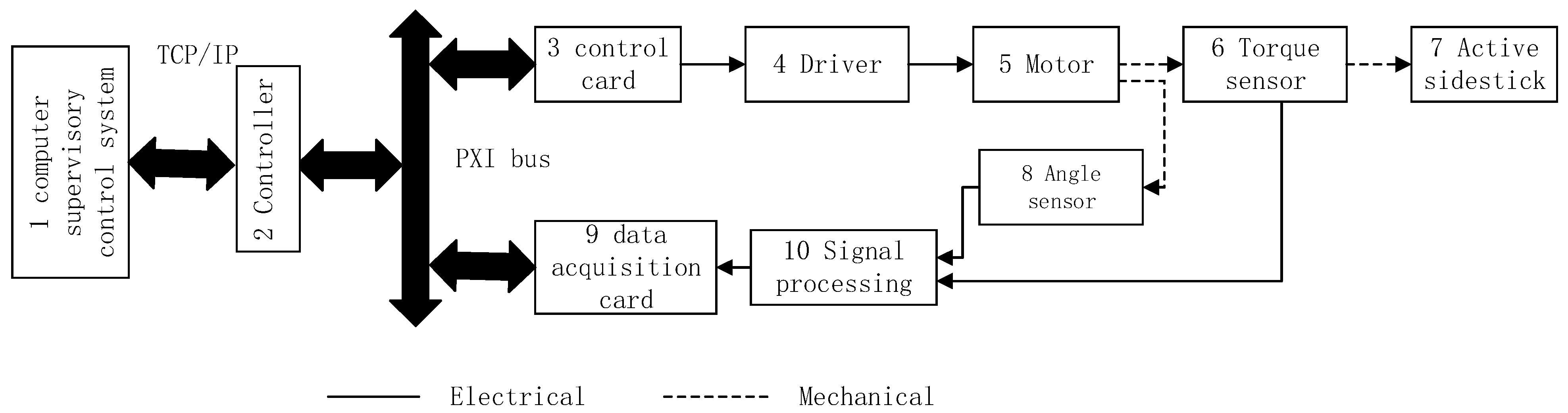
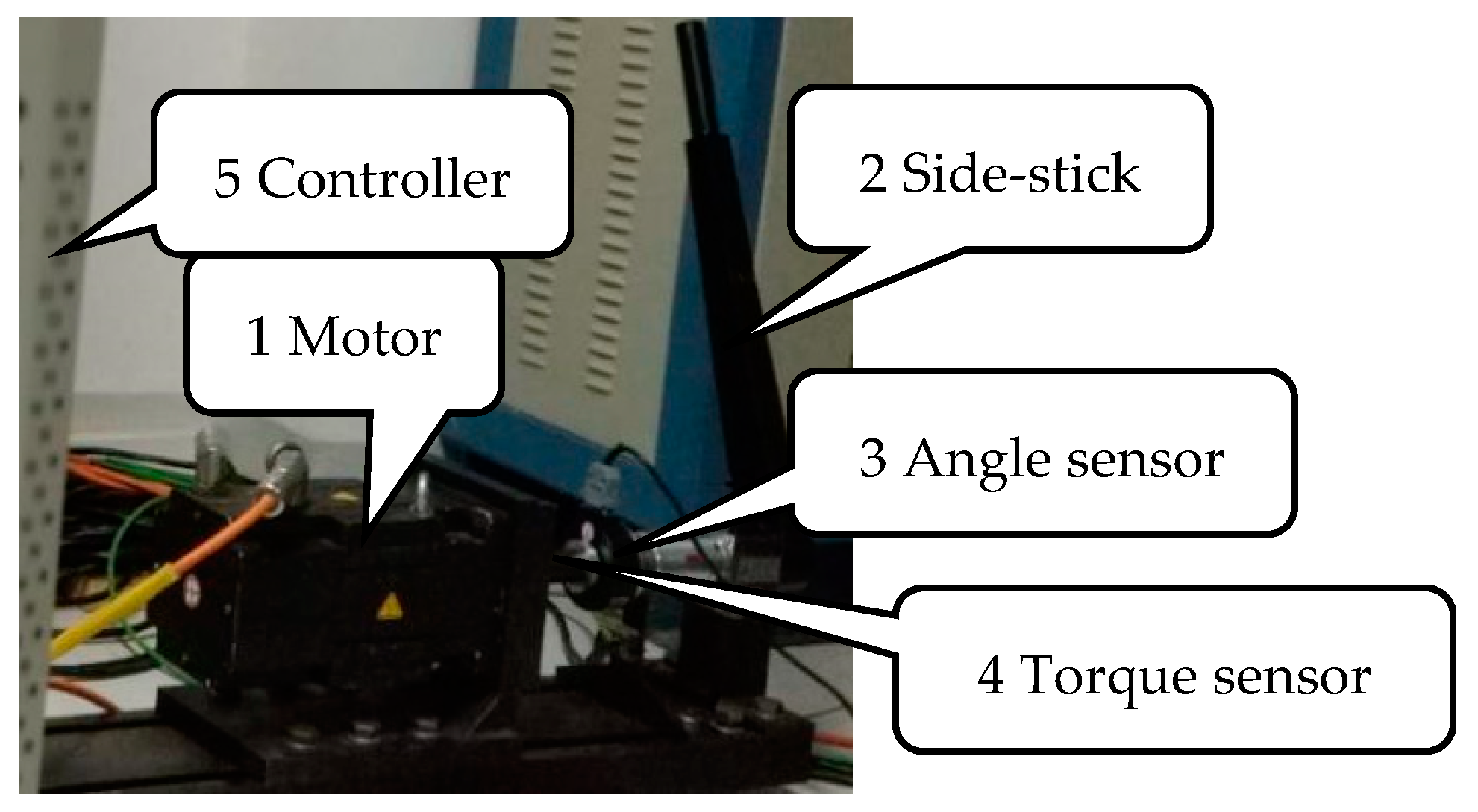
5.1. Test Scheme

The test platform is as Figure 24.

The master computer 1 adopts a Linghua RK610/M342 industrial computer, which provides a cabinet solution based on M342 and supports high-performance industrial automation applications. The actuator 5 uses the Kormogan torque motor, which can achieve long-term stall; in order to realize real-time control of the torque motor, NI-CRIO architecture is used as the real-time controller 2 [27,28]. The specific controller model is NI-CRIO-9104. NI sub-board card selection is as follows:

(1)

NI-9263 is used for the instruction of the analog output module as the actuator. NI-9263 is a 4-channel 100 kS/s synchronous update analog output module. The 0-1 and 4-5 channel output torque and position analog signals are used in this test bench.

(2)

NI-9215 is an analog input card with 16 channels, 100 kS/s/channel, 16 bits, ±10 V analog input module. NI-9215 can perform differential simulation inputs.

(3)

Counters and timers are NI-9411. The NI-9215 counter input module has 8 channels and can directly collect digital quantity. Users can configure it to be differential or single-ended.

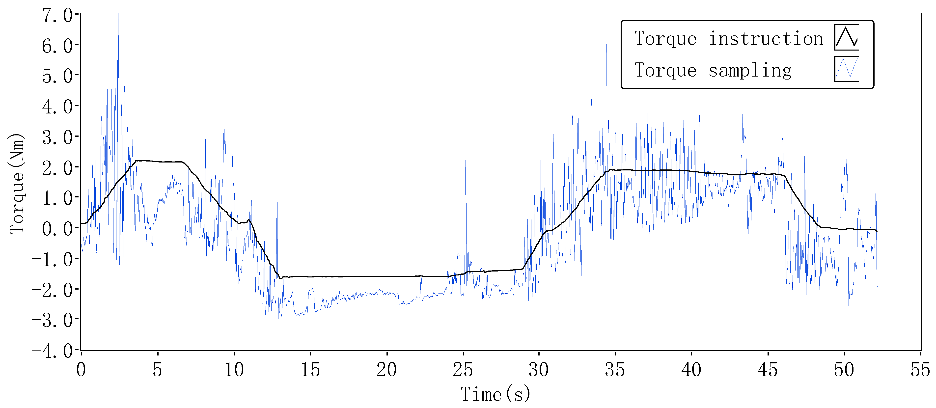
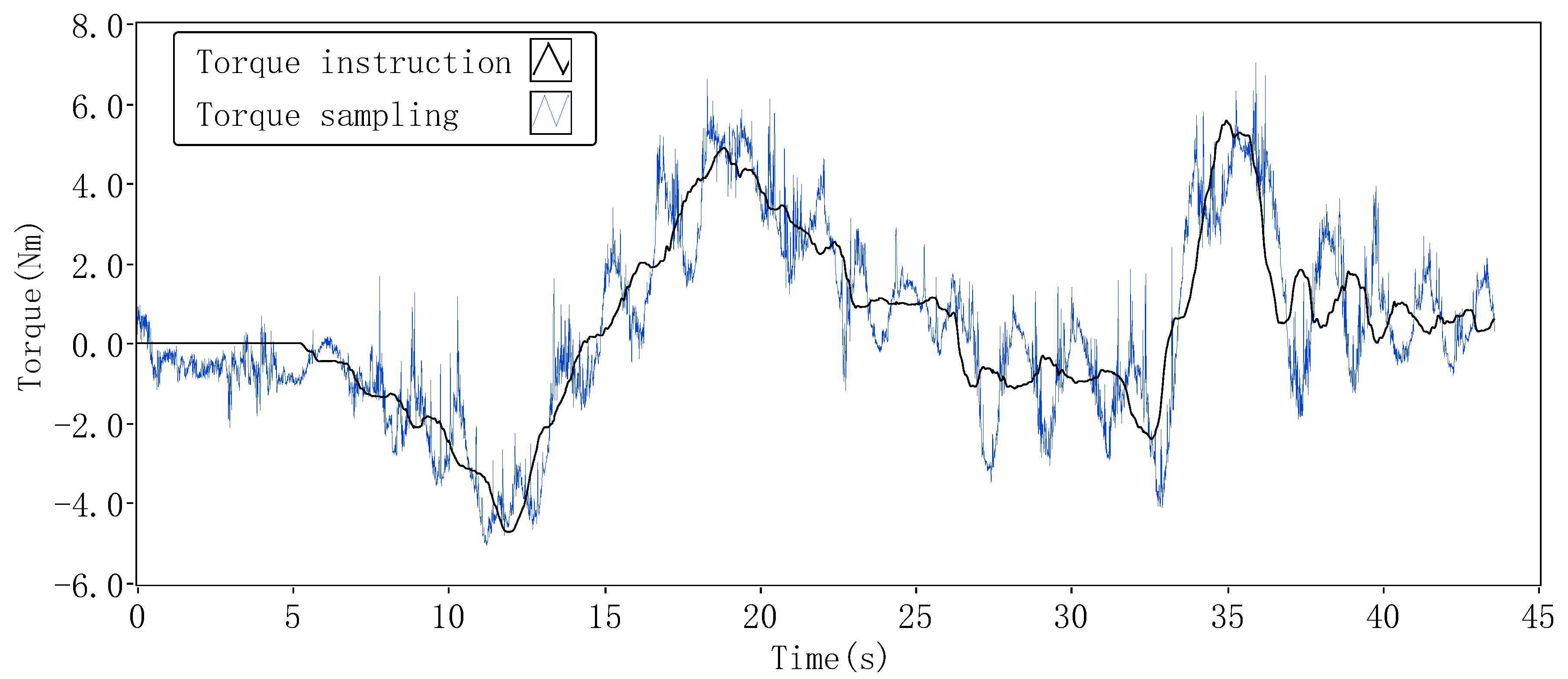
5.2. Test Results

The test bench and control cabinet of the control system are shown in Figure 25.

In the experiment, we simulated the process of active control. According to tactile information, people manipulate the driving side-stick 2, moving the side-stick 2 in accordance with certain rules. The input force command of the position system is related to the displacement of the driving side-stick. The active control controller controls the output of the accurate tracking input command. The process of manually-manipulating the driving side-stick is similar to the spring. We tested different stiffnesses, as shown in the Figure 26, Figure 27, Figure 28 and Figure 29.

From the Figure 26, Figure 27, Figure 28 and Figure 29, it can be seen that the control force of the side-stick depends on the real-time position of the side-stick manipulated by the hand. When the side-stick is in zero position, the side-stick remains unchanged. When the hand exerts a thrust in one direction to the side bar, the side bar will swing in this direction and react to the hand; when pushed to one side limit, the hand loosens the side-stick, the side-stick will automatically bounce back to the initial position, and the ejection acceleration is linearly related to the angle of the side-stick rotation. The test results showed that the position system can accurately track the input instructions under different stiffnesses, and the system has good robust stability.

6. Summary and Conclusions

This paper, based on the background of fly-by-wire control, takes the active side-stick control as the research object. Firstly, the control characteristics of the system were discussed and analyzed based on the mathematical model of the ACS, and the closed loop controller of the system was further designed. The compensation strategy of the structural invariance principle was used to compensate for the interference torque generated by the coupling of the two systems. Secondly, on the basis of the compensation model, the robust control idea was introduced to transform the system stability index into the robustness index, which improved the robustness of the system. Finally, a test platform was built to compare the simulation results with the test curves. The main research results of this paper are as follows:

(1)

Different to traditional fly-by-wire technology, this paper proposes the design principle of the side-stick in an artificial feel system. The ACS was divided into position system and torque system for modeling and analysis, respectively. The two subsystems were coupled to form a comprehensive system, and the transfer functions of the command channel and the interference channel were solved. The comprehensive model of the subsystem and the coupling state was simulated and analyzed.

(2)

The servo characteristics of the system were analyzed, and the position closed-loop system and the torque closed-loop system were preliminarily designed. At the same time, the factors that cause the instability of the system were discussed, and the influences of inertia, clearance, damping and stiffness on the system were also discussed. The causes of the interference torque were studied. The structure invariance principle was adopted to compensate for the torque closed-loop system, and the software adjustment strategy was used to compensate for the torque generated by the interference.

(3)

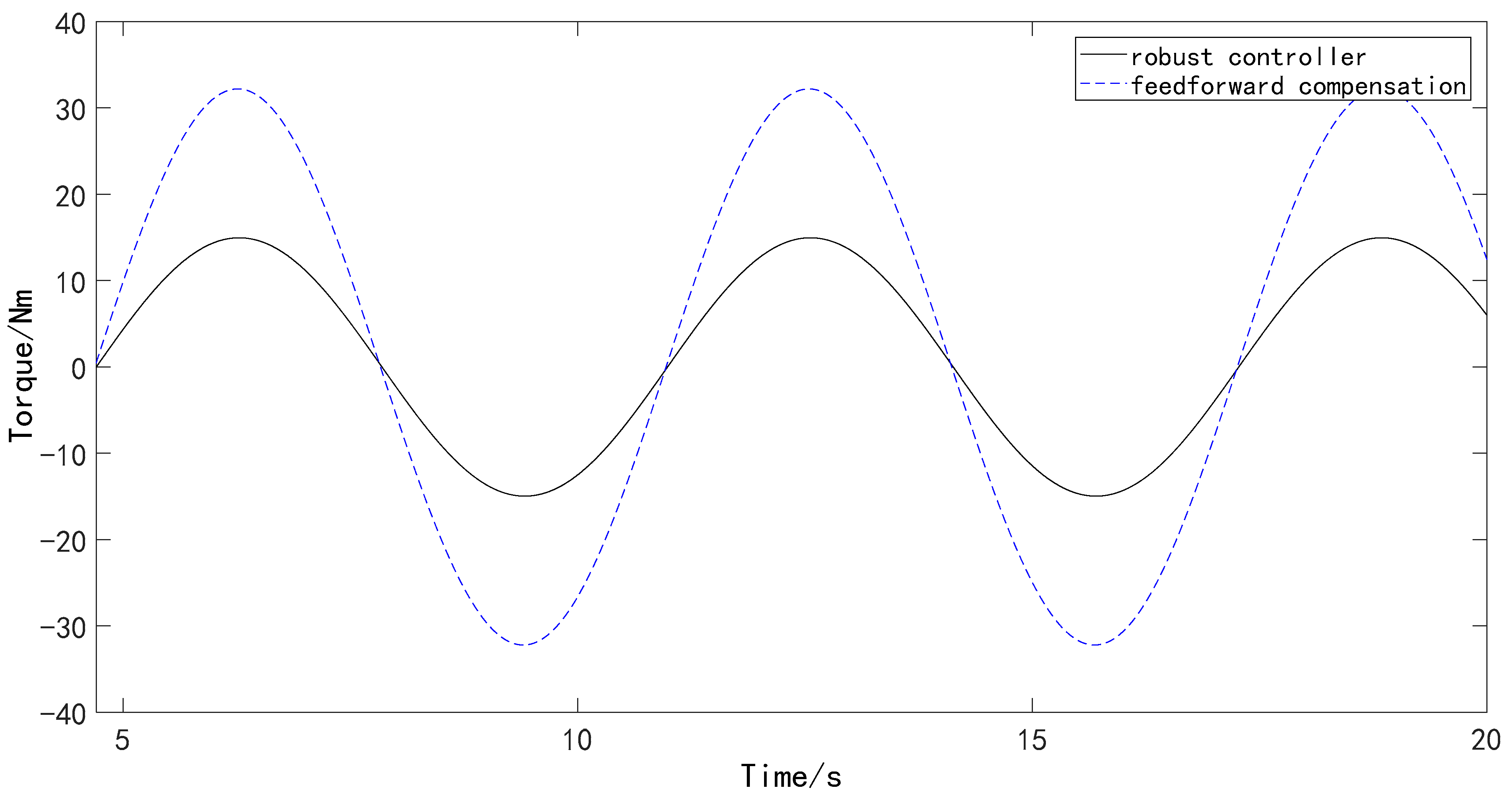
This paper proposes a robust control method for active side-stick manipulation based on $H_{\infty }$. The designed torque closed-loop system has uncertainty and external perturbation, which is in line with the applicable environment of the robust controller. It proved that the effect of robust $H_{\infty }$ control on suppressing external disturbance of the system was good. Compared with dynamic compensation, the effect of suppressing disturbance is more obvious, and the robustness of the system is significantly enhanced.

This paper can be referred to in the research of artificial feel systems for active side-sticks.

References

- Burns, B.R.A. Fly-by-wire and control configured rewards and risks. Aeronaut. J. 2016, 79, 51–58. [Google Scholar]
- Dlamini, Z.; Jones, T. Fly-by-wire robustness to flight dynamics change under horizontal stabiliser damage. Aeronaut. J. 2016, 120, 1005–1023. [Google Scholar] [CrossRef]
- Rushby, J.M. Formal specification and verification of a fault-masking and transient-recovery model for digital flight-control systems. In Proceedings of the International Symposium on Formal Techniques in Real-Time and Fault-Tolerant Systems, Nijmegen, The Netherlands, 8–10 January 1992; pp. 237–257. [Google Scholar]
- David, M.; Euan, M.; Stewart, H. MIMO Sliding Mode Attitude Command Flight Control System for a Helicopter. In Proceedings of the AIAA Guidance, Navigation, and Control Conference and Exhibit, San Francisco, CL, USA, 15–18 August 2005. [Google Scholar]
- Wang, X.; Wang, S.; Yao, B. Adaptive robust torque control of electric load simulator with strong position coupling disturbance. Int. J. Control. Autom. Syst. 2013, 11, 325–332. [Google Scholar] [CrossRef]
- Jiao, Z.; Hua, Q.; Wang, X.; Wang, S. Compound control of electro-hydraulic load simulator. Chin. J. Mech. Eng. 2002, 38, 685–689. [Google Scholar] [CrossRef]
- Qing, H.; Zongxia, J. CRNN neural network control of the load simulator. Chin. J. Mech. Eng. 2003, 38, 15–19. [Google Scholar]
- Jiao, Z.; Hua, Q. RBF neural network control on electrohydraulic load simulator. Chin. J. Mech. Eng. 2003, 39, 10–14. [Google Scholar] [CrossRef]
- Guo, C.; Yang, R.; Zhang, P.; Fu, M. The control algorithm improving performance of electric load simulator. In Proceedings of the Seventh International Conference on Electronics and Information Engineering. International Society for Optics and Photonics, Nanjing, China, 17–18 September 2016. [Google Scholar]
- Guo, B.Z.; Zhao, Z.L. Active Disturbance Rejection Control for Nonlinear Systems: An Introduction; John Wiley & Sons: Hoboken, NJ, USA, 2016. [Google Scholar]
- Liu, Y.; Gao, X.; Pei, Z. Research of Impact Load in Large Electrohydraulic Load Simulator. Math. Probl. Eng. 2014, 2014, 1–7. [Google Scholar] [CrossRef]
- Fergani, S.; Allias, J.F.; Briere, Y.; Defay, F. A novel structure design and control strategy for an aircraft active sidestick. In Proceedings of the Control & Automation, Athens, Greece, 21–24 June 2016. [Google Scholar]
- Chang, J.; Shen, D.; Chen, D. Active Disturbance Rejection Control Tuned by Whale Optimization Algorithm for Electric Loading System. In Proceedings of the 39th Chinese Control Conference, Shenyang, China, 27–29 July 2020; pp. 1150–1154. [Google Scholar]
- Li, T.; Zhang, B.; Feng, Z.; Zheng, B. Robust Control with Engineering Applications. Math. Probl. Eng. 2014, 2014, 567672. [Google Scholar] [CrossRef]
- Wang, C.; Hou, Y.; Liu, R.; Gao, Q.; Hou, R. Control of the Electric Load Simulator Using Fuzzy Multiresolution Wavelet Neural Network with Dynamic Compensation. Shock. Vib. 2016, 2016, 3574214. [Google Scholar] [CrossRef]
- Chenggong, L.; Hongtao, J.; Zongxia, J. Mechanism and suppression of extraneous torque of motor driver load simulator. J. Beijing Univ. Aeronaut. Astronaut. 2006, 32, 204–208. [Google Scholar]
- Otto, C.; Petr, H. Adaptive fuzzy sliding mode control for electro-hydraulic servo mechanism. Expert Syst. Appl. 2012, 39, 10269–10277. [Google Scholar]
- Zhang, H.; Yang, S. On energy-to-peak filtering for nonuniformly sampled nonlinear systems: A Markovian Jump System Approach. IEEE Trans. FUZZY Syst. 2014, 22, 212–222. [Google Scholar] [CrossRef]
- Lü, S.-S.; Lin, H.; Fan, M.D. Electric loading system with multiclosed-loop control. Electr. Mach. Control. 2015, 19, 16–22. [Google Scholar]
- Bae, H.R.; Daniel, C.L.; Alyanak, E. Sequential Subspace Robustness Assessment and Sensitivity Analysis. AIAA J. 2016, 55, 1–14. [Google Scholar]
- Ting, Z.; Rui, L. Improved Tracking Differentiator and Fuzzy PID for Electric Loading System. In Proceedings of the 4th International Conference on Mechatronics, Materials, Chemistry and Computer Engineering, Xi’an, China, 12–13 December 2015. [Google Scholar]
- Stîngă, F.; Marian, M.; Selișteanu, D. Robust Estimation-Based Control Strategies for Induction Motors. Complexity 2020, 2020, 9235701. [Google Scholar] [CrossRef]
- Shuai, Y.U.; Dong-Po, B. Research of Robust Control for Electro-Hydraulic Servo Loading System. Meas. Control. Technol. 2009, 28, 58–61. [Google Scholar]
- Wang, J.; Liang, L.; Zhang, S.; Ye, Z.; Li, H. Application of Control Based on Mixed Sensitivity in the Electro-hydraulic Load Simulator. In Proceedings of the International Conference on Mechatronics & Automation, Harbin, China, 5–8 August 2007. [Google Scholar]
- Kosut, R.L.; Emami-Naeini, A.; Salzwedel, H. Robust Control of Flexible Spacecraft. J. Guid. Control. Dyn. 1971, 6, 104–111. [Google Scholar] [CrossRef]
- Choi, J.; Ryu, H.S.; Kim, C.W.; Choi, J.H. An efficient and robust contact algorithm for a compliant contact force model between bodies of complex geometry. Multibody Syst. Dyn. 2010, 23, 99–120. [Google Scholar] [CrossRef]
- Gu, Da.; Zhang, Da.; Liu, Yi. Robust Parametric Control of Lorenz System via State Feedback. Complexity 2020, 2020, 6548142. [Google Scholar] [CrossRef]
- Monmasson, E.; Cirstea, M.N. Design Methodology for Industrial Control Systems—A Review. IEEE Trans. Ind. Electron. 2007, 54, 1824–1842. [Google Scholar] [CrossRef]