Article

Influence of Boundary Impedance of 3D Cavity on Targeted Energy Transfer between a Damped Acoustic Mode and a Nonlinear Membrane Absorber

School of Automotive Studies, Tongji University, Shanghai 201804, China
*
Author to whom correspondence should be addressed.
Machines 2022, 10(10), 841; https://doi.org/10.3390/machines10100841
Submission received: 11 August 2022 / Revised: 14 September 2022 / Accepted: 21 September 2022 / Published: 22 September 2022
(This article belongs to the Special Issue Noise and Vibration Control in Dynamic Systems)

Abstract

:
In order to apply the nonlinear energy sink (NES) to reduce the low-frequency noise inside a 3D acoustic cavity with an impedance boundary, a two degrees-of-freedom (DOF) dynamic model of the coupled system of one damped acoustic mode of a regular 3D acoustic cavity and a nonlinear membrane absorber as the NES is established. The damping coefficient of the acoustic mode is obtained based on the finite element analysis method and the relationship of the boundary impedance and the absorption coefficient of the cavity. Based on the set-up of the system, the damping coefficient of the acoustic mode is determined. The frequency responses and the targeted energy transfer (TET) phenomenon of the coupled system are analyzed, and the theoretical and numerical results of the frequency responses of the system are in good agreement with the experimental ones. The effects of the wall impedance of the cavity on the optimal TET are discussed. With the increase in the impedance ratio of the wall, the amplitude of the acoustic displacement plateau decreases, and the frequency bandwidth of the plateau and the two thresholds of the optimal TET interval of the excitation increase. It provides a comprehensive theoretical model and experimental basis for the application of NES in the actual complex structure and provides a reliable design method and control strategy for controlling vehicle interior low-frequency broadband noise.

1. Introduction

The nonlinear energy sink (NES) utilized to control the low-frequency vibration and noise can be coupled with the multi-modes of primary system due to the nonlinear stiffness. Resonance capture phenomenon occurs between the primary system and the NES under a certain external excitation so that the vibration energy of the primary structure is irreversibly transferred to the NES, quickly concentrated in the NES and dissipated by the NES damping, namely the targeted energy transfer (TET), to achieve the effect of attenuating the energy of the primary system [1,2]. Compared with the traditional noise reduction means by adding damping materials, the NES is simple in structure and lightweight [3]. Therefore, the NES technology is an ideal technique to control vehicle interior low-frequency noise. From the theoretical and numerical view, many methods, such as the complexification-averaging (CX-A) method [4], complexification-averaging combined with multiple-scales analysis method [5,6,7], Runge–Kutta method [8,9], harmonic balance method (HBM) [10] and other methods, are used to analyze nonlinear normal modes (NNM) and resonance capture of the systems. Under a certain external excitation, the resonance peak is efficiently reduced when the coupling system presents in a quasi-periodic motion, namely strongly modulated response (SMR) [11,12]. The peak reduction can occur in a wide frequency bandwidth due to the characteristics of the NES. However, the NES only operates efficiently in a limited range of the excitation amplitude [13,14].
In terms of noise suppression in 1D acoustic cavity, in 2006, Cochelin et al. [15] first applied a NES to noise reduction. They used a rubber membrane with nonlinear stiffness acting as a NES to control the low-frequency noise in a tube (1D acoustic system). Experimental results showed that the nonlinear membrane achieves one-way energy transfer from the 1D acoustic cavity with rigid wall to the NES. Bellet et al. [16] used a tube with variable length, a coupling box, a membrane, and a holding device that can adjust the membrane radius and pre-stress to experiment and found that a specific membrane absorber can tune itself to different acoustic systems at the resonance frequency of the systems. The irreversible energy transfer phenomenon can be observed in the system under both free vibration and forced vibration, and the energy transfer rate can reach more than 80%. Later, they pointed out that because the characteristics that different membranes are activated in turn and behave relatively independently, using several NES can extend the energy transfer range and the efficiency of TET. A new zone of TET is created when there are different membranes in parallel, and the existing zone is extended when there are similar membranes in parallel [17].
In terms of noise suppression in the 3D acoustic cavity, Shao et al. [10] used HBM and the asymptotic numerical method to study the TET phenomenon of a simple two degrees-of-freedom (DOF) dynamic system and obtained the excitation threshold for the beginning of TET given by an analytical formula. According to the analysis of the simple two DOFs system, the TET between a membrane NES and the undamped acoustic mode of the cavity with rigid walls were studied, and a two DOFs system model consisting of the single-order undamped acoustic mode of the cavity and the single NES was established. The NES can effectively suppress the noise of the acoustic cavity, which is validated by the experimental method [18]. In the follow-up research, they studied the suppression effect of the two acoustic modes with a single NES. The research showed that the NES can simultaneously suppress the amplitudes of the two acoustic modes [19]. In addition, they explored the coupling characteristics between different numbers of NES and acoustic cavity modes. For two similar membranes, the desired working zone is extended with the suppressed amplitude of the vibration response unchanged. For two different membranes, in addition to the extension of the desired working zone, the response appears as two plateaus with different values [20]. Subsequently, based on the research of the two DOFs system, they optimized the material parameters, structure size parameters and installation position of the NES that affect the TET phenomenon [21]. Then they deduced the theoretical formula of the beginning and ending TET thresholds and analyzed the influence of the pre-stress on the first mode frequency of the membrane and the frequency bandwidth of the TET [22]. Bryk et al. [23] combined active feedback control with passive NES and proposed a new type of electroacoustic nonlinear membrane absorber which can change the system resonance frequency by controlling the feedback gain and adjust the threshold that triggers off the TET phenomenon. Furthermore, they used the singular perturbation method around a 1:1 resonance to find the slow critical manifold of the system and its dependence on the control loop gain in the voltage and current driving mode, and obtained the conditions for the generating of SMR. In a concrete room with the absorber, the sound pressure level measured at the first-order mode of the room around 43 Hz is attenuated by 8 dB [24]. However, for the application of NES to reduce low-frequency noise inside acoustic medium with acoustic materials, such as the vehicle interior, the comparison of the influence of wall with and without acoustic materials for the TET phenomenon was only studied by the experimental method. The theoretical model of the system for the modal damping coefficient of the cavity was always fixed and not changed with different boundary impedance ratios. The effect of the boundary impedance of acoustic materials to the modal damping coefficient of the cavity and the TET characteristics of NES is ignored for the theoretical model of the system.
In this paper, to consider the influence of the boundary impedance of the 3D cavity for the practical use of the membrane NES, a comprehensive theoretical model of the two DOFs system with one damped acoustic mode of the 3D cavity and one nonlinear membrane is built. The damping coefficient of the acoustic mode is determined to analyze the influence for the TET phenomenon. Then the frequency responses of the system are analyzed, and the experimental results validate the theoretical and numerical ones based on the set-up of the system. The effects of the wall impedance of the cavity on the optimal TET are finally performed.

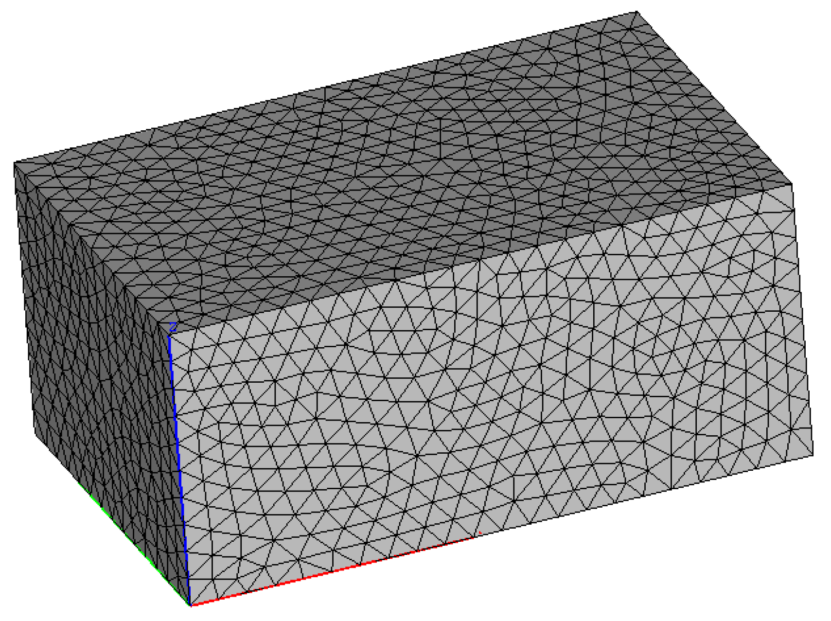
2. Description of the System

The schema of the system in this paper is shown in Figure 1. A parallelepiped acoustic cavity as the acoustic medium and the main system and a nonlinear membrane as the NES that is mounted on one wall of the cavity are considered. The dimensions of the 3D cavity are L x = 2.2   m , L y = 1.4   m and L z = 1   m , and the position of the membrane is marked as ( x m , y m , z m ). The six walls of the 3D cavity shown are rigid. Ω is the internal volume of the acoustic cavity, S is the surface of the acoustic cavity, S 1 is the surface of the acoustic cavity without the surface of the membrane, S m is the surface of the membrane, and S = S 1 + S m .
The acoustic wave equation of the 3D cavity in the time domain is as follows:
1 c 0 2 2 p r , t t 2 2 p r , t = 0 ,
where p r , t is the acoustic pressure at a point inside the cavity, r is the position vector, and c 0 is the sound velocity.
The acoustic pressure p r of a damped mode marked by the integers l ,   m ,   n is given by
p r = p r x , y , z , t = ψ l m n D x , y , z p t .
The damped mode shape of the cavity ψ l m n D is defined as follows:
ψ l m n D x , y , z = cos ( ω l c 0 x + i k 0 c 0 β x 0 ω l ) cos ( ω m c 0 y + i k 0 c 0 β y 0 ω m ) cos ( ω n c 0 z + i k 0 c 0 β z 0 ω n ) ,
where k 0 is the wave number of the mode, β j 0 ,   j = x ,   y ,   z is the specific impedance ratio of each wall of the cavity, and ω k ,   k = l ,   m ,   n is the angular frequency and is equal to the following form:
ω k c 0 = k π L j 2 i ε k k 0 β j 0 + β j L j L j ,
and for ε k ,   k = l ,   m ,   n , when k = 0 ,   ε k = 1 ; when k 0 ,   ε k = 2 .
The first damped mode of the cavity ψ 100 D ( l = 1 ,   m = 0 ,   n = 0 ) is here taken and a Rayleigh–Ritz reduction to one DOF system is performed by using the damped mode shape ψ 100 D as a single shape function for p r and for the test function δ p r = ψ 100 D x , y , z δ p t :
Ω ( 1 c 0 2 2 p r t 2 δ p r 2 p r δ p r ) d Ω = 0 .
By considering the impedance boundary condition of the cavity and based on Green’s theorem, Ω 2 p r δ p r d Ω becomes
Ω 2 p r δ p r d Ω = Ω 2 δ p r p r d Ω + s p r δ p r n d S s δ p r p r n d S ,
where,
Ω 2 δ p r p r d Ω = Ω 2 p r δ p r d Ω = Ω p r δ p r d Ω δ p r n = 0 s δ p r p r n d S = s 1 δ p r p r n d S 1 + S m δ p r p r n d S m .
By introducing Equations (6) and (7), Equation (5) is expanded to the following form:
Ω 1 c 0 2 2 p r t 2 δ p r d Ω + Ω p r δ p r d Ω s 1 δ p r p r n d S 1 S m δ p r p r n d S m = 0 .
Then, the one DOF system of the acoustic mode is obtained as follows (see the Appendix B for the equation of the system):
m a p ¨ + k a p + ρ 0 2 c 0 2 S m ψ 100 D x m , y m , z m 2 q ¨ = 0 ,
where q t and p t are the transversal displacement amplitude of the membrane center (direction O x in Figure 1) and the acoustic pressure amplitude, respectively. S m is the surface area of the membrane. m a and k a are the modal mass and stiffness of the system, respectively.
For the equation of the membrane NES, the one DOF model of Bellet [12] is taken in this paper and is of the following form:
m m q ¨ + k 1 ( f 1 f 0 ) 2 q + η q ˙ + k 3 2 η q 2 q ˙ + q 3 S m ψ 100 D x m , y m , z m 2 p = 0 ,
with
S m = π R 2 , m m = ρ m h S m 3 ,   k 1 = 1.015 4 π 5 E h 3 36 1 υ 2 R 2 , k 3 = 8 π E h 3 1 υ 2 R 2 , f 0 = 1 2 π 1.015 4 π 4 E h 2 12 1 υ 2 ρ m R 4   ,
where m m ,   k 1 ,   k 3 ,   f 0 ,   f 1 are the mass, linear stiffness, nonlinear stiffness, and first resonance frequency without pre-stress and with pre-stress of the membrane, respectively. x m , y m , z m is the position of the membrane center.
By introducing a viscous term as the acoustic damping with a coefficient c a and an external forcing term F u t on the acoustic cavity and replacing the acoustic pressure amplitude p t by the acoustic displacement amplitude u t = p t / ρ 0 c 0 ω 100 , the final system with two DOFs of the damped mode ψ 100 D and the nonlinear membrane is as follows:
m a u ¨ + c a u ˙ + k a u + R a q ¨ = F u t m m q ¨ + k 1 ζ q + η q ˙ + k 3 2 η q 2 q ˙ + q 3 R q u = 0 ,
with
c a = m a k a Q , R a = ρ 0 c 0 S m ψ 100 D x m , y m , z m 2 ω 100 , F u t = F p t ρ 0 c 0 ω 100 ,     ζ = ( f 1 f 0 ) 2 , R q = ρ 0 c 0 ω 100 S m ψ 100 D x m , y m , z m 2   .
According to the system (12), it can be seen that the terms of coupling are R a and R q , which are determined by the placement of the membrane ( x m , y m , z m ). If the center of the membrane is on the nodal line of the acoustic mode ψ 100 D , the coupling between u t and q t is null. In [21], the physical parameters and the positions of the membrane were also analyzed. It was shown that a large range of values for the radius and thickness of the membrane could affect the TET phenomenon, and the position of the membrane should be far from the nodal line of the cavity for the TET phenomenon. Here, the position of the membrane is set by ( x m = L x , y m = L y / 4 , z m = L z / 4 ) and the parameters of the membrane are chosen as shown in Table 1 and are fixed along the paper. The units of F u t , F r e q u e n c y and t i m e are N, Hz and s, respectively, and the unit of the amplitude of u t and q t is m.

3. Acoustic Damping Coefficient

The normal mode and normal frequency of the acoustic cavity with boundary impedance are both complex, and the imaginary part is related to the specific impedance ratio β . Meanwhile, the real part of the acoustic impedance is represented by the resistance term, and the imaginary part is represented by inductance and capacitance [25,26]. Similarly, in the system of the flat panel vibration absorber, the real part of acoustic impedance is the damping term, and the imaginary part is the mass and stiffness term [27]. Based on the dynamic model of the damped acoustic mode, the modal mass m a and modal stiffness k a of the acoustic mode of the cavity are both functions of the specific impedance ratio β , namely, that the boundary impedance changes the resonance frequency f of the acoustic cavity, as shown in Figure 2. As the specific impedance ratio β increases, the modal mass m a of the acoustic cavity increases, while the modal stiffness k a of the acoustic cavity decreases. Thus, the resonance frequency f of the acoustic cavity decreases.
There are many acoustic materials, called sound packages, inside of a vehicle, such as carpets and seats, and the sound absorption coefficients are usually tested. According to the definition of specific impedance ratio β and sound absorption coefficient α of the acoustic material, the estimated relationship between β and α can be obtained as follows:
β = ρ 0 c 0 Z α = 4 Z ρ 0 c 0 Z ρ 0 c 0 + 1 2 β = 2 4 α 2 + 2 4 α 2 4 .
According to Equation (14), the relationship between each specific impedance ratio β x 0 ,   β y 0 , β z 0 , β x L x , β y L y , β z L z and each sound absorption coefficient α x 0 ,   α y 0 , α z 0 , α x L x , α y L y , α z L z of the six walls of the cavity is determined. Then, the sound absorption coefficient α v of the cavity is obtained:
α v = j = 1 6 α j s j j = 1 6 s j ,
where α j and s j represent each sound absorption coefficient and each surface area of the six walls of the cavity, respectively.
Here, it is assumed that the same acoustic material is added to the six walls of the cavity. The sound absorption coefficients α x 0 ,   α y 0 , α z 0 , α x L x , α y L y , α z L z of the six walls of the cavity are equal to the sound absorption coefficient α v of the cavity. By using the finite element analysis method, the finite element model of the cavity without the membrane NES is built as shown in Figure 3, whose element size is 0.1 m. The forced frequency response of the cavity is shown in Figure 4 under white noise excitation with 1 N and with the sound absorption coefficient of the cavity α v = 0.01 . Based on the half-power bandwidth method, the quality factor Q of the cavity can be obtained for α v = 0.01 . Then the corresponding modal damping coefficient is obtained by c a = m a ω 100 / Q . Thus, the relationship of the boundary impedance and the modal damping coefficient of the cavity is determined. Table 2 shows the different sound absorption coefficients of the acoustic materials and the corresponding quality factor and specific impedance ratio.

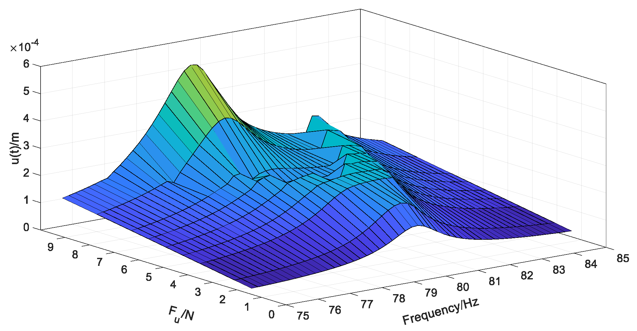
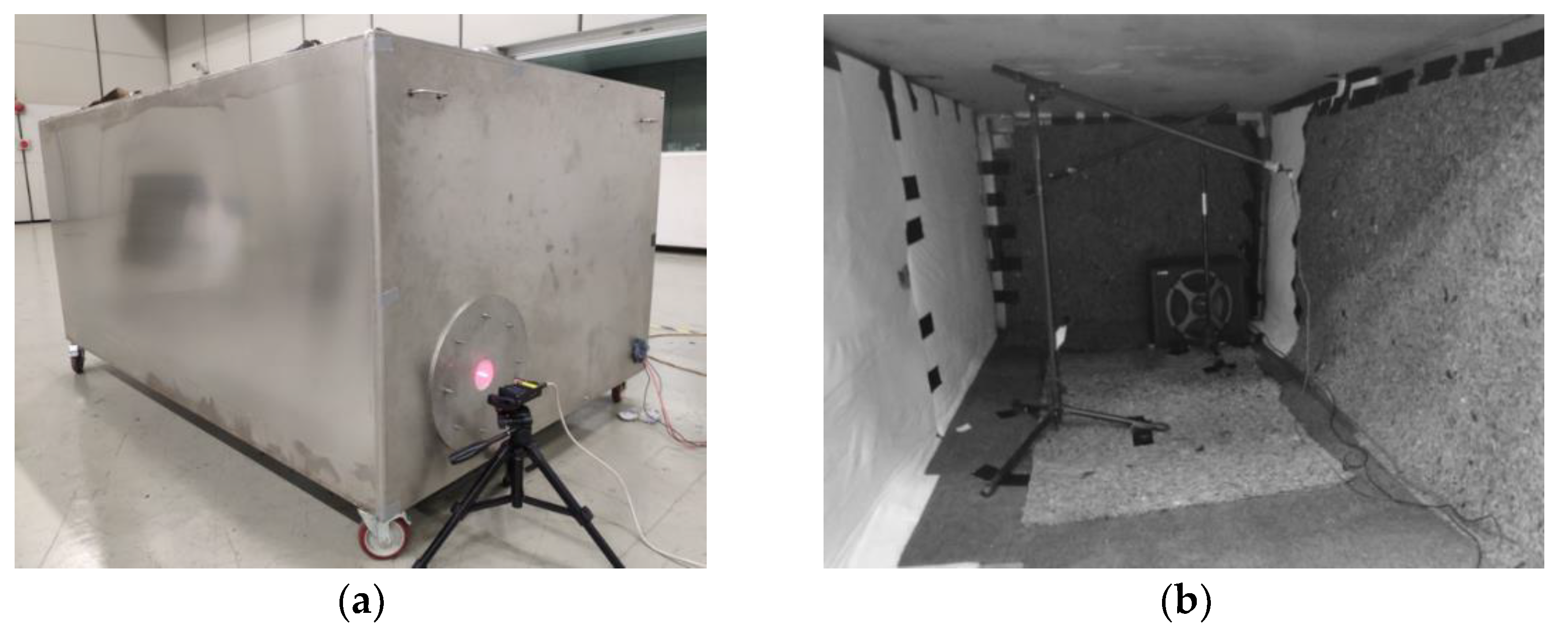
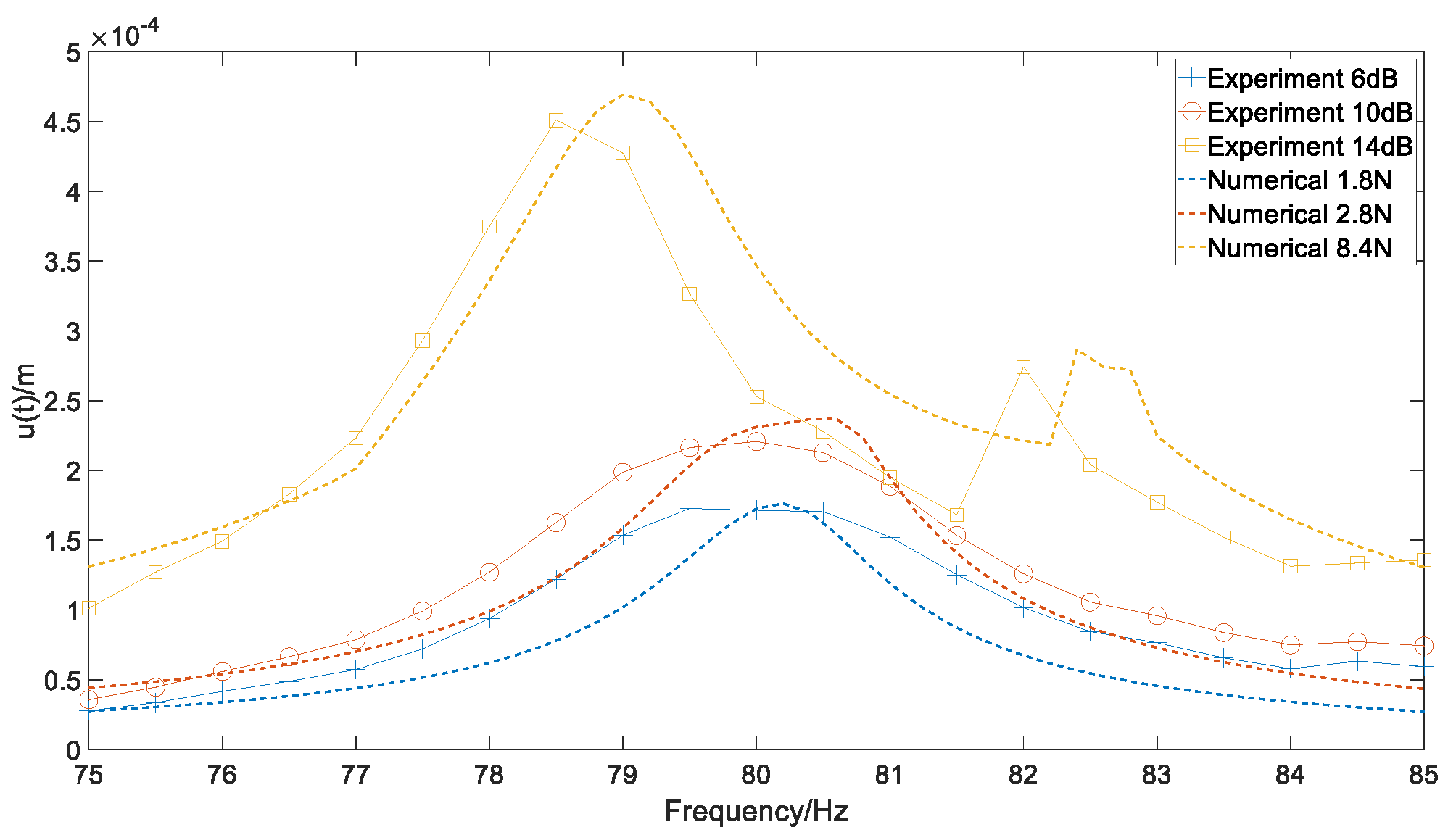
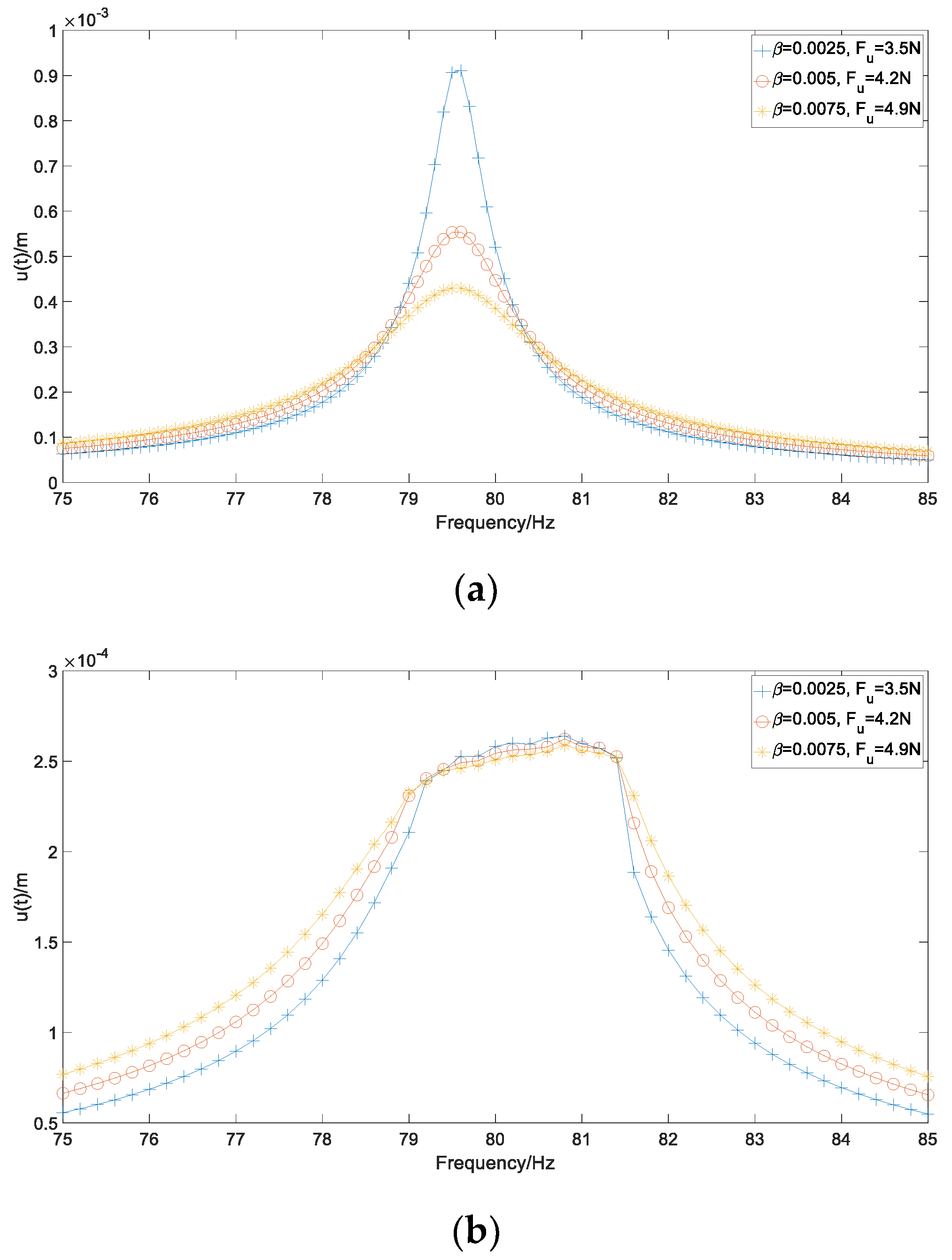
4. Experimental and Numerical Forced Responses of the System

Based on the experimental set-up in Reference [18], the quality factors Q of the cavity with the acoustic materials are measured Q = 52.47 . The corresponding modal damping coefficient and each specific impedance ratio are obtained by c a = m a k a Q = 18.98 and β x 0 ,   β y 0 , β z 0 , β x L x , β y L y , β z L z = β = 0.0063 . The 4th and 5th order Runge–Kutta methods are used to perform the forced responses of the system (12). The frequency f of the excitation is varied inside the range [75 Hz, 85 Hz] with an interval of Δ f = 0.2 Hz, and the forcing amplitude F u of the excitation is varied in the range [1.4 N, 9.1 N]. The excitation with each combination of frequency and amplitude in the selected range is applied inside the cavity, and the maximum value of the acoustic displacement amplitude u t is taken as the frequency response amplitude, as shown in Figure 5 and Figure 6.
(1)
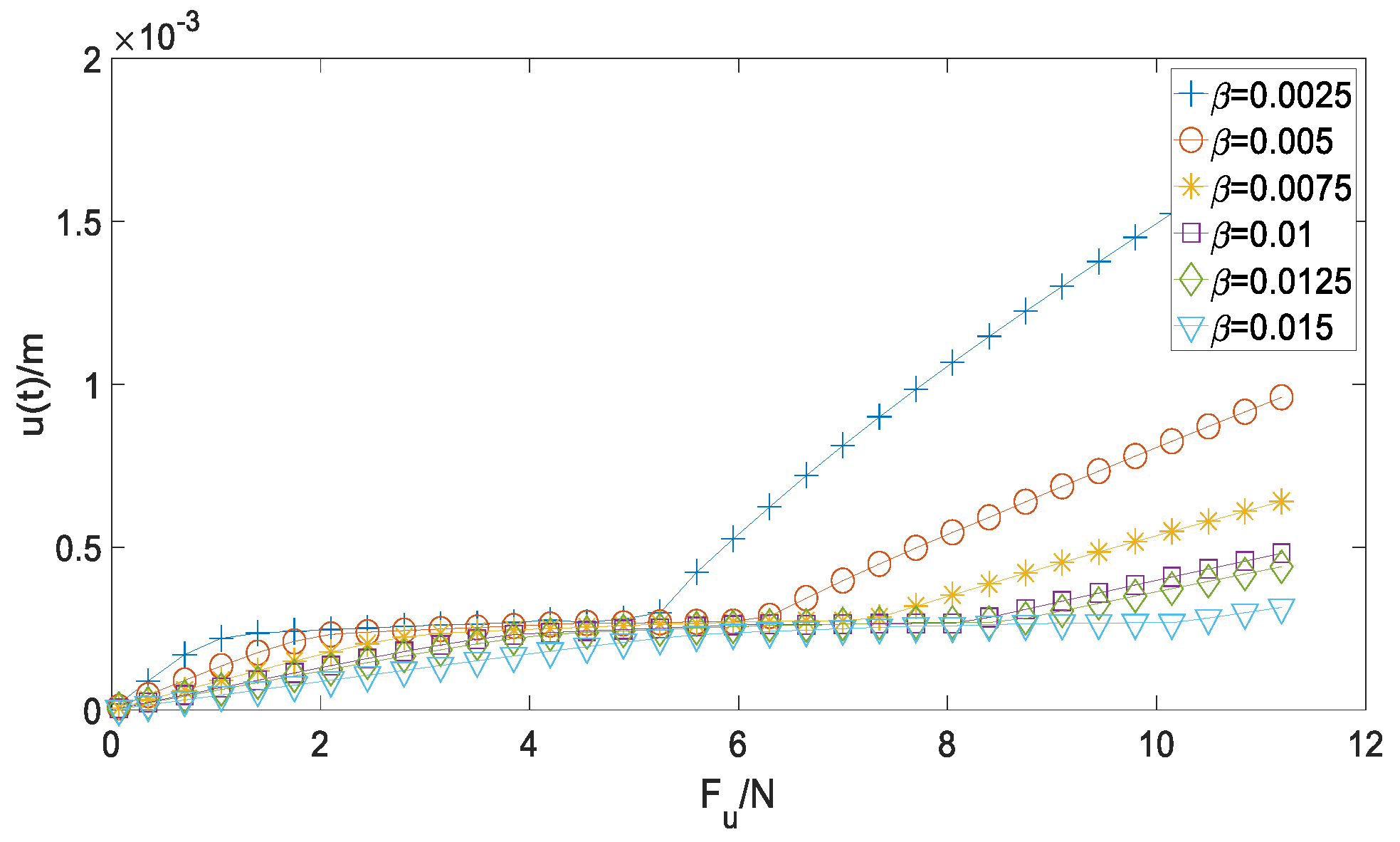
In the low excitation amplitude range, such as F u = 2.1   N , the acoustic displacement amplitude u t has a single resonance peak at the resonance frequency, and the response amplitude of u t increases with the increase in the excitation amplitude.
(2)
In the medium excitation amplitude range, such as F u = 4 . 9   N , the forced response u t produces a plateau with an amplitude of about 2.2 × 10 4 2.7 × 10 4 m within a certain frequency range, and the resonance peak is suppressed and disappears, where the regime of responses of the system is SMR. This range starts with the appearance of the plateau and ends with the appearance of another new resonance peak. As the forcing excitation amplitude increases, the energy triggers the working threshold of the membrane NES in a wider frequency band near the resonance frequency, and the frequency range of the plateau gradually increases.
(3)
In the high excitation amplitude range, such as F u = 7.7   N , the forced response has a new resonance peak below the original resonance frequency, which is higher than the resonance peak under the low forcing excitation. In addition, the plateau of the forced response u t appearing near the resonance frequency under the forcing excitation with medium amplitude begins to disappear. As the forcing excitation amplitude increases, the second resonance peak increases further, and the plateau of the forced response u t near the resonance frequency basically disappears.
Based on the experimental set-up in Reference [18] as shown in Figure 7, where the loud speaker and power amplifier are located, the microphones and the laser rangefinder are used to be the acoustic source and measure the acoustic pressure response inside the cavity and the displacements of the membrane, respectively. The experimental forced responses of the acoustic displacement u t under the excitation amplitudes of 6, 10, and 14 dB are obtained as shown in Figure 8. The experimental results are consistent with the numerical analysis results. When the excitation amplitude is 10 dB, there is a plateau of u t with an amplitude about 2.4 × 10 4 m. From the experimental point of view, it is verified that within a certain excitation amplitude and frequency range, the TET phenomenon of the system occurs, and the forms of the response curves are consistent, which validates the theoretical model of the system.

5. Influence of the Wall Impedance for the TET

The relationship of the threshold of the TET interval according to the damping coefficient μ = c a / m a was studied in Reference [18], where the specific impedance ratio β of the wall was not considered for the system (12). According to the sound absorption coefficient of the vehicle interior in the low frequency, the sound absorption coefficient α v of the cavity is here taken in the range [0.01, 0.06]. Then the specific impedance ratio β is obtained in the range [0.0025, 0.015]. According to the frequency response of the acoustic displacement u t inside the acoustic cavity shown in Figure 5 and Figure 6, the highest amplitude of u t under each excitation amplitude is taken to obtain the relationship between the maximum acoustic displacement amplitude u t and the excitation amplitude F u . Considering the actual application inside vehicle, the optimal TET interval corresponding to the excitation amplitude with the specific impedance ratio β in the range [0.0025, 0.015] is analyzed as shown in Figure 9. It can be intuitively seen that the plateau value of u t corresponds to a range of the excitation amplitude. As the specific impedance ratio β increases, namely when an acoustic material with higher sound absorption is added to the boundary wall of the cavity, the two thresholds of the optimal TET interval and the frequency bandwidth of the optimal TET increase, and the plateau value of u t decreases.
For the increase in the initial threshold of the optimal TET with the higher specific impedance ratio β , because the modal damping coefficient c a of the cavity increases, the larger excitation amplitude is needed to reach the plateau value for the resonance peak. It can be also seen for the forced responses of u t without the membrane NES, as shown in Figure 10a, where for β = 0.0075 , the resonance peak of u t under the higher excitation amplitude F u = 4.9   N is lower than that for β = 0.005 under the smaller excitation amplitude F u = 4.2   N . Meanwhile, for the increase in the frequency bandwidth of the optimal TET, the frequency bandwidth of u t with and without the membrane NES at the plateau value 2.4 × 10 4 m is larger for the higher specific impedance ratio β , as shown in Figure 10.

6. Conclusions

In this paper, a two DOFs dynamic model of the coupled system, which is composed of a single damped acoustic mode of a regular 3D cavity and a membrane NES is established. The relationship of the boundary impedance and the modal damping coefficient of the cavity is determined based on the finite element analysis method and the relationship of the boundary impedance and the absorption coefficient of the cavity. Then for the set-up of the system with acoustic materials, the damping coefficient of the acoustic mode and the equation of the system are determined by considering the boundary impedance ratio. The forced responses and the TET phenomenon of the system are analyzed by the theoretical and numerical methods, which show that the results of the frequency responses of the system are in good agreement. From the perspective of the optimal TET interval of the membrane, which is defined by the excitation amplitude range corresponding to the plateau, the influence of specific impedance ratio on the optimal TET is explored. The results show that with the increase in the specific impedance ratio, the two thresholds of the optimal TET interval and the frequency bandwidth of the optimal TET increase, and the plateau value of the responses decreases.

Author Contributions

J.S.: Conceptualization, Funding acquisition, Methodology, Investigation, Writing—original draft, Writing—review and editing. Q.L.: Investigation, Writing—original draft, Writing—review and editing. T.Z.: Investigation, Writing—original draft. X.W.: Conceptualization, Methodology. All authors have read and agreed to the published version of the manuscript.

Funding

This research was supported by the National Nature Science Foundations of China (Grant No. 51805372), Shanghai Science and Technology Program (Grant No. 21DZ1208704) and the Natural Science Foundation of Shanghai (Grant No. 18ZR1440900).

Institutional Review Board Statement

Not applicable.

Informed Consent Statement

Not applicable.

Data Availability Statement

The datasets generated during and/or analyzed during the current study are available from the corresponding author on reasonable request.

Acknowledgments

The authors sincerely thank the National Nature Science Foundations of China, Shanghai Science and Technology Program and the Natural Science Foundation of Shanghai for providing us with a good platform. And all individuals included in this section have consented to the acknowledgement.

Conflicts of Interest

All persons who meet authorship criteria are listed as authors, and all authors certify that they have participated sufficiently in the work to take public responsibility for the content, including participation in the concept, design, analysis, writing, or revision of the manuscript. Furthermore, each author certifies that this material or similar material has not been and will not be submitted to or published in any other publication.

Appendix A

SymbolUnitDescription
C l , C m , C n Corresponding normal mode in direction O x , O y , O z
c a Nm/sAcoustic damping
c 0 m/sSound wave velocity
E MPaModulus of the membrane
F u NExternal force amplitude
f 0 HzFirst resonance frequency without pre-stress of the membrane
f 1 HzFirst resonance frequency with pre-stress of the membrane
h mThickness of the membrane
k a N/mModal stiffness of the system
k 0 m 1 Wave number of the mode
k 1 N/mLinear stiffness of the membrane
k 3 N / m 3 Nonlinear stiffness of the membrane
L x mLength of the cavity
L y mWidth of the cavity
L z mHeight of the cavity
l m n Normal modes
m a kgModal mass of the system
m m kgMass of the membrane
n Boundary normal vector
p PaAcoustic pressure
p r PaAcoustic pressure of a damped mode
Q Quality factor
q mTransversal displacement amplitude of the membrane center
r mPosition vector
R mRadius of the membrane
S m 2 Surface of the cavity
S m m 2 Surface of the membrane
S 1 m 2 Surface of the cavity without the surface of the membrane
t sTime
u mAcoustic displacement amplitude
x m , y m , z m mPosition of the membrane center
Z Acoustic impedance
α Sound absorption coefficient
α v Sound absorption coefficient of the cavity
α x 0 ,   α y 0 , α z 0 , α x L x , α y L y , α z L z Sound absorption coefficient of each wall of the cavity
β Specific impedance ratio
β x 0 ,   β y 0 , β z 0 , β x L x , β y L y , β z L z Specific impedance ratio of each wall of the cavity
δ p r Test function
ε l , ε m , ε n Coefficients
η Damping of the membrane
ν Poisson ratio of the membrane
ρ m kg / m 3 Density of the membrane
ρ 0 kg / m 3 Air density
ψ l m n D Damped mode shape of the cavity
Ω m 3 Internal volume of the cavity
ω l ,   ω m , ω n rad/sNormal angular frequency

Appendix B

Based on Equation (4), the component in direction O x of the normal frequency is
( ω l c 0 ) 2 = ( l π L x ) 2 i ε l k 0 ( β x 0 + β x L x ) L x .
Then, Equation (A1) is marked as follows:
ω l c 0 = ( l π L x ) 2 i ε l k 0 ( β x 0 + β x L x ) L x b x + i c x .
The corresponding normal mode in direction O x could be given by
C l ( x ) = cos ( ω l c 0 x + i k 0 c 0 β x 0 ω l )           = cos [ ( b x + i c x ) x + i k 0 β x 0 b x i c x ( b x + i c x ) ( b x i c x ) ]           = cos [ ( b x + i c x ) x + i k 0 β x 0 b x b x 2 + c x 2 + k 0 β x 0 c x b x 2 + c x 2 ]           = cos ( A x x + P x i + Q x ) ,
where
A x = b x + i c x , P x = k 0 β x 0 b x b x 2 + c x 2 , Q x = k 0 β x 0 c x b x 2 + c x 2 .
Then, the integral of C l 2 x and ( C l x ) 2 in the interval 0 , L x is given by
0 L x C l 2 ( x ) d x = 0 L x cos 2 ( A x x + P x i + Q x ) d x     = 0 L x 1 + cos ( 2 A x x + 2 P x i + 2 Q x ) 2 d x     = L x 2 + sin ( 2 A x L x + 2 P x i + 2 Q x ) sin ( 2 P x i + 2 Q x ) 4 A x     = L x 2 + B x , 0 L x ( C l ( x ) ) 2 d x = 0 L x sin 2 ( A x x + P x i + Q x ) d x             = 0 L x 1 cos ( 2 A x x + 2 P x i + 2 Q x ) 2 d x             = L x 2 sin ( 2 A x L x + 2 P x i + 2 Q x ) sin ( 2 P x i + 2 Q x ) 4 A x             = L x 2 B x ,
where
B x = sin ( 2 A x L x + 2 P x i + 2 Q x ) sin ( 2 P x i + 2 Q x ) 4 A x .
According to the inference in direction O x , the following results for the components in direction O y and O z are obtained:
ω m c 0 = ( m π L y ) 2 i ε m k 0 ( β y 0 + β y L y ) L y b y + i c y ω n c 0 = ( n π L z ) 2 i ε n k 0 ( β z 0 + β z L z ) L z b z + i c z C m ( y ) = cos ( ω m c 0 y + i k 0 c 0 β y 0 ω m ) = cos ( A y y + P y i + Q y ) C n ( z ) = cos ( ω n c 0 z + i k 0 c 0 β z 0 ω n ) = cos ( A z z + P z i + Q z ) 0 L y C m 2 ( y ) d y = L y 2 + B y   ,   0 L y ( C m ' ( y ) ) 2 d y = L y 2 B y 0 L z C n 2 ( z ) d z = L z 2 + B z   ,   0 L z ( C n ' ( z ) ) 2 d z = L z 2 B z .
For Equation (8), each term of the integral can be got. For the term of Ω 1 c 0 2 2 p r t 2 δ p r d Ω , it is given by
Ω 1 c 0 2 2 p r t 2 δ p r d Ω = Ω 1 c 0 2 ψ l m n D p ¨ ψ l m n D δ p d Ω                     = 1 c 0 2 p ¨ δ p Ω ( ψ l m n D ) 2 d Ω                     = 1 c 0 2 p ¨ δ p 0 L x C l 2 ( x ) d x 0 L y C m 2 ( y ) d y 0 L z C n 2 ( z ) d z                     = 1 c 0 2 ( L x 2 + B x ) ( L y 2 + B y ) ( L z 2 + B z ) p ¨ δ p                     = D 1 p ¨ δ p .
For the term of Ω p r δ p r d Ω , based on the definition of gradient, the following equations are given by
ψ l m n D = ψ l m n D x i + ψ l m n D y j + ψ l m n D z k , ψ l m n D x = C l ( x ) C m ( y ) C n ( z ) = A x sin ( A x x + P x i + Q x ) cos ( A y y + P y i + Q y ) cos ( A z z + P z i + Q z ) ψ l m n D y = C l ( x ) C m ( y ) C n ( z ) = A y cos ( A x x + P x i + Q x ) sin ( A y y + P y i + Q y ) cos ( A z z + P z i + Q z ) ψ l m n D z = C l ( x ) C m ( y ) C n ( z ) = A z cos ( A x x + P x i + Q x ) cos ( A y y + P y i + Q y ) sin ( A z z + P z i + Q z ) .
Then,
Ω p r δ p r d Ω = p δ p Ω ψ l m n D ψ l m n D d Ω = p δ p 0 L x 0 L y 0 L z [ ( C l ( x ) C m ( y ) C n ( z ) ) 2 + ( C l ( x ) C m ( y ) C n ( z ) ) 2       + ( C l ( x ) C m ( y ) C n ( z ) ) 2 ] d x d y d z = [ A x 2 ( L x 2 B x ) ( L y 2 + B y ) ( L z 2 + B z ) + A y 2 ( L x 2 + B x ) ( L y 2 B y ) ( L z 2 + B z )       + A z 2 ( L x 2 + B x ) ( L y 2 + B y ) ( L z 2 B z ) ] p δ p = D 2 p δ p .
For the term s 1 δ p r p r n d S 1 , the expanded formula is given by
s 1 δ p r p r n d S 1 = σ y z δ p r p r n x = 0 , L x d y d z                                                     + σ z x δ p r p r n y = 0 , L y d z d x + σ x y δ p r p r n z = 0 , L z d x d y .
To consider the effect of boundary impedance condition, the Robin boundary condition is used:
ψ l m n D x | x = 0 + i k 0 β x 0 ψ l m n D ( 0 , y , z ) = 0 ,       ψ l m n D x | x = L x i k 0 β x L x ψ l m n D ( L x , y , z ) = 0 ψ l m n D y | y = 0 + i k 0 β y 0 ψ l m n D ( x , 0 , z ) = 0 ,       ψ l m n D y | y = L y i k 0 β y L y ψ l m n D ( x , L y , z ) = 0 ψ l m n D z | z = 0 + i k 0 β z 0 ψ l m n D ( x , y , 0 ) = 0 ,       ψ l m n D z | z = L z i k 0 β z L z ψ l m n D ( x , y , L z ) = 0 .
The effects of the y z plane, the z x plane and the x y plane are given by
σ y z δ p r p r n | x = 0 , L x d y d z = i k 0 β x L x p δ p σ y z ( ψ l m n D ( L x , y , z ) ) 2 d y d z i k 0 β x 0 p δ p σ y z ( ψ l m n D ( 0 , y , z ) ) 2 d y d z = i k 0 p δ p [ β x L x C l 2 ( x = L x ) β x 0 C l 2 ( x = 0 ) ] 0 L y C m 2 ( y ) d y 0 L z C n 2 ( z ) d z = i k 0 ( L y 2 + B y ) ( L z 2 + B z ) [ β x L x cos 2 ( A x L x + P x i + Q x ) β x 0 cos 2 ( P x i + Q x ) ] p δ p = i D y z p δ p , σ z x δ p r p r n | y = 0 , L y d z d x = i k 0 β y L y p δ p σ z x ( ψ l m n D ( x , L y , z ) ) 2 d z d x i k 0 β y 0 p δ p σ z x ( ψ l m n D ( x , 0 , z ) ) 2 d z d x = i k 0 p δ p [ β y L y C m 2 ( y = L y ) β y 0 C m 2 ( y = 0 ) ] 0 L z C n 2 ( z ) d z 0 L x C l 2 ( x ) d x = i k 0 ( L x 2 + B x ) ( L z 2 + B z ) [ β y L y cos 2 ( A y L y + P y i + Q y ) β y 0 cos 2 ( P y i + Q y ) ] p δ p = i D z x p δ p , σ x y δ p r p r n | z = 0 , L z d x d y = i k 0 β z L z p δ p σ x y ( ψ l m n D ( x , y , L z ) ) 2 d x d y i k 0 β z 0 p δ p σ x y ( ψ l m n D ( x , y , 0 ) ) 2 d x d y = i k 0 p δ p [ β z L z C n 2 ( z = L z ) β z 0 C n 2 ( z = 0 ) ] 0 L x C l 2 ( x ) d x 0 L y C m 2 ( y ) d y = i k 0 ( L x 2 + B x ) ( L y 2 + B y ) [ β z L z cos 2 ( A z L z + P z i + Q z ) β z 0 cos 2 ( P z i + Q z ) ] p δ p = i D x y p δ p .
Then,
S 1 δ p r p r n d S 1 = i ( D y z + D z x + D x y ) p δ p .
For the term S m δ p r p r n d S m , based on the boundary condition ρ 0 2 w t 2 = p r n S m , it is given by
S m δ p r p r n d S m = S m ρ 0 2 w t 2 ψ l m n D ( x m , y m , z m ) δ p d S m                                                                 = ρ 0 ψ l m n D ( x m , y m , z m ) δ p S m q ¨ ( 1 r 2 R 2 ) d S m                                                                 = ρ 0 ψ l m n D ( x m , y m , z m ) q ¨ δ p 0 2 π d θ 0 R ( 1 r 2 R 2 ) ρ d ρ                                                                 = ρ 0 π R 2 ψ l m n D ( x m , y m , z m ) 2 q ¨ δ p .
Then, Equation (8) becomes
D 1 p ¨ + [ D 2 i ( D y z + D z x + D x y ) ] p + ρ 0 π R 2 ψ l m n D ( x m , y m , z m ) 2 q ¨ = 0 .
By multiplying the coefficient ρ 0 c 0 2 and adding the acoustic damping term c a p ˙ and the forcing term F p t , the one DOF system of the acoustic mode is given by
m a p ¨ + c a p ˙ + k a p + ρ 0 2 c 0 2 S m ψ l m n D ( x m , y m , z m ) 2 q ¨ = F p ( t ) ,
with m a = D 1 ρ 0 c 0 2 and k a = D 2 i D y z + D z x + D x y ρ 0 c 0 2 .

References

  1. Gendelman, O.; Manevitch, L.I.; Vakakis, A.F.; M’Closkey, R. Energy pumping in nonlinear mechanical oscillators: Part I—Dynamics of the underlying hamiltonian systems. J. Appl. Mech. 2001, 68, 34–41. [Google Scholar] [CrossRef]
  2. Vakakis, A.F.; Gendelman, O. Energy pumping in nonlinear mechanical oscillators: Part II—Resonance capture. J. Appl. Mech. 2001, 68, 42–48. [Google Scholar] [CrossRef]
  3. Shao, J.; Yang, J.; Wu, X.; Zeng, T. Nonlinear energy sink applied for low-frequency noise control inside acoustic cavities: A review. J. Low Freq. Noise Vib. Act. Control 2020, 40, 1453–1472. [Google Scholar] [CrossRef]
  4. Lee, Y.S.; Kerschen, G.; Vakakis, A.F.; Panagopoulos, P.; Bergman, L.; McFarland, D.M. Complicated dynamics of a linear oscillator with a light, essentially nonlinear attachment. Physica D 2005, 204, 41–69. [Google Scholar] [CrossRef]
  5. Gendelman, O.V.; Starosvetsky, Y.; Feldman, M. Attractors of harmonically forced linear oscillator with attached nonlinear energy sink (Part I & II). Nonlinear Dyn. 2008, 51, 31–46. [Google Scholar]
  6. Starosvetsky, Y.; Gendelman, O.V. Vibration absorption in systems with a nonlinear energy sink: Nonlinear damping. J. Sound Vib. 2009, 324, 916–939. [Google Scholar] [CrossRef]
  7. Vaurigaud, B.; Savadkoohi, A.T.; Lamarque, C.H. Targeted energy transfer with parallel nonlinear energy sinks. Part I: Design theory and numerical results. Nonlinear Dyn. 2011, 66, 763–780. [Google Scholar] [CrossRef]
  8. Mariani, R.; Bellizzi, S.; Cochelin, B.; Herzog, P.; Mattei, P.O. Toward an adjustable nonlinear low frequency acoustic absorber. J. Sound Vib. 2011, 330, 5245–5258. [Google Scholar] [CrossRef]
  9. Bitar, D.; Gourdon, E.; Lamarque, C.H.; Collet, M. Shunt loudspeaker using nonlinear energy sink. J. Sound Vib. 2019, 456, 254–271. [Google Scholar] [CrossRef]
  10. Shao, J.; Cochelin, B. Theoretical and numerical study of targeted energy transfer inside an acoustic cavity by a non-linear membrane absorber. Int. J. Non-Linear Mech. 2014, 64, 85–92. [Google Scholar] [CrossRef]
  11. Starosvetsky, Y.; Gendelman, O. Dynamics of a strongly nonlinear vibration absorber coupled to a harmonically excited two-degree-of-freedom system. J. Sound Vib. 2008, 312, 234–256. [Google Scholar] [CrossRef]
  12. Bellet, R.; Cochelin, B.; Herzog, P.; Mattei, P.O. Experimental study of targeted energy transfer from an acoustic system to a nonlinear membrane absorber. J. Sound Vib. 2010, 329, 2768–2791. [Google Scholar] [CrossRef]
  13. Vakakis, A.F. Passive nonlinear targeted energy transfer. Philos. Trans. R. Soc. A (Math. Phys. Eng. Sci.) 2018, 376, 20170132. [Google Scholar] [CrossRef]
  14. Lu, Z.; Wang, Z.; Zhou, Y.; Lu, X. Nonlinear dissipative devices in structural vibration control: A review. J. Sound Vib. 2018, 423, 18–49. [Google Scholar] [CrossRef]
  15. Cochelin, B.; Herzog, P.; Mattei, P.O. Experimental evidence of energy pumping in acoustics. C. R. Mec. 2006, 334, 639–644. [Google Scholar] [CrossRef]
  16. Bellizzi, S.; Côte, R.; Pachebat, M. Responses of a two degree-of-freedom system coupled to a nonlinear damper under multi-forcing frequencies. J. Sound Vib. 2013, 332, 1639–1653. [Google Scholar] [CrossRef]
  17. Bellet, R.; Cochelin, B.; Côte, R.; Mattei, P.O. Enhancing the dynamic range of targeted energy transfer in acoustics using several nonlinear membrane absorbers. J. Sound Vib. 2012, 331, 5657–5668. [Google Scholar] [CrossRef]
  18. Shao, J.; Luo, Q.; Deng, G.; Zeng, T.; Yang, J.; Wu, X.; Jin, C. Experimental study on influence of wall acoustic materials of 3D cavity for targeted energy transfer of a nonlinear membrane absorber. Appl. Acoust. 2021, 184, 108342. [Google Scholar] [CrossRef]
  19. Shao, J.; Zeng, T.; Wu, X. Study of a nonlinear membrane absorber applied to 3D acoustic cavity for low frequency broadband noise control. Materials 2019, 12, 1138. [Google Scholar] [CrossRef]
  20. Wu, X.; Shao, J.; Cochelin, B. Study of targeted energy transfer inside three-dimensional acoustic cavity by two nonlinear membrane absorbers and an acoustic mode. J. Vib. Acoust. 2016, 138, 031017. [Google Scholar] [CrossRef]
  21. Wu, X.; Shao, J.; Cochelin, B. Parameters design of a nonlinear membrane absorber applied to 3D acoustic cavity based on targeted energy transfer (TET). Noise Control Eng. J. 2016, 64, 99–113. [Google Scholar] [CrossRef]
  22. Shao, J.; Zeng, T.; Wu, X.; Yang, J. Influence of the pre-stress of the nonlinear membrane absorber for targeted energy transfer applied to 3D acoustic cavity. J. Braz. Soc. Mech. Sci. Eng. 2020, 42, 557. [Google Scholar] [CrossRef]
  23. Bryk, P.Y.; Bellizzi, S.; Côte, R. Experimental study of a hybrid electro-acoustic nonlinear membrane absorber. J. Sound Vib. 2018, 424, 224–237. [Google Scholar] [CrossRef]
  24. Bryk, P.Y.; Côte, R.; Bellizzi, S. Targeted energy transfer from a resonant room to a hybrid electro-acoustic nonlinear membrane absorber: Numerical and experimental study. J. Sound Vib. 2019, 460, 114868. [Google Scholar]
  25. Guo, X.; Lissek, H.; Fleury, R. Improving sound absorption through nonlinear active electroacoustic resonators. Phys. Rev. Appl. 2020, 13, 014018. [Google Scholar] [CrossRef]
  26. Tao, J.; Jing, R.; Qiu, X. Sound absorption of a finite micro-perforated panel backed by a shunted loudspeaker. J. Acoust. Soc. Am. 2014, 135, 231–238. [Google Scholar] [CrossRef]
  27. Lee, Y.Y.; Li, Q.S.; Leung, A.Y.T.; Su, R.K.L. The jump phenomenon effect on the sound absorption of a nonlinear panel absorber and sound transmission loss of a nonlinear panel backed by a cavity. Nonlinear Dyn. 2012, 69, 99–116. [Google Scholar] [CrossRef]
Figure 1. Schema of the system of a 3D cavity and a nonlinear membrane.
Machines 10 00841 g001
Figure 2. The modal mass m a , modal stiffness k a and resonance frequency f of the acoustic mode according to the specific impedance ratio β .
Machines 10 00841 g002
Figure 3. The finite element model of the cavity.
Machines 10 00841 g003
Figure 4. The forced frequency response of the cavity under the excitation 1 N and with the sound absorption coefficient of the cavity α v = 0.01 .
Machines 10 00841 g004
Figure 5. The numerical responses of the acoustic displacement u t under the excitation amplitude range [1.4 N, 9.1 N] and the frequency range [75 Hz, 85 Hz].
Machines 10 00841 g005
Figure 6. The periodic responses surface according to the excitation amplitude and the excitation frequency.
Machines 10 00841 g006
Figure 7. The experimental set-up. (a) The cavity, the membrane and the laser rangefinder. (b) The cavity interior and locations of the excitation and microphone with wall acoustic materials.
Machines 10 00841 g007
Figure 8. The comparison between the experimental and numerical responses of the acoustic displacement u t of the system.
Machines 10 00841 g008
Figure 9. The optimal TET interval of the membrane NES with the specific impedance ratio β in the range [0.0025, 0.015].
Machines 10 00841 g009
Figure 10. The forced responses of the system with different specific impedance ratio β under different excitation amplitude. (a) Without the membrane NES. (b) With the membrane NES.
Machines 10 00841 g010
Table 1. The parameters of the system.
Air   density   ρ 0 1.3   kg / m 3 Density   of   the   membrane   ρ m 1000   kg / m 3
Sound   velocity   c 0 350   m / s Thickness   of   the   membrane   h 0.00011 m
Density   of   the   membrane   ρ m 0.001 s Radius   of   the   membrane   R 0.04 m
Poisson   ratio   of   the   membrane   ν 0.47 Modulus   of   the   membrane   E 1.58 MPa
Table 2. The different sound absorption coefficient of acoustic materials and the corresponding quality factor and specific impedance ratio.
α0.010.020.030.040.050.06
Q132.6866.3443.9833.0330.2721.99
β0.00250.0050.00750.010.01250.015
Publisher’s Note: MDPI stays neutral with regard to jurisdictional claims in published maps and institutional affiliations.

