Article

Bayesian Regularization Algorithm Based Recurrent Neural Network Method and NSGA-II for the Optimal Design of the Reflector

1
Shanghai Institute of Technical Physics, Chinese Academy of Sciences, Shanghai 200083, China
2
University of Chinese Academy of Sciences, Beijing 100049, China
3
Key Laboratory of Infrared Detection and Imaging Technology, Shanghai Institute of Technical Physics, Chinese Academy of Sciences, Shanghai 200083, China
*
Author to whom correspondence should be addressed.
Machines 2022, 10(1), 63; https://doi.org/10.3390/machines10010063
Submission received: 27 November 2021 / Revised: 10 January 2022 / Accepted: 14 January 2022 / Published: 15 January 2022
(This article belongs to the Special Issue Precision Measurement and Machines)

Abstract

:
The optical-mechanical system of a space camera is composed of several complex components, and the effects of several factors (weight, gravity, modal frequency, temperature, etc.) on its system performance need to be considered during ground tests, launch, and in-orbit operation. In order to meet the system specifications of the optical camera system, the dimensional parameters of the optical camera structure need to be optimized. There is a highly nonlinear functional relationship between the dimensional parameters of the optical machine structure and the design indexes. The traditional method takes a significant amount of time for finite element calculation and is less efficient. In order to improve the optimization efficiency, a recurrent neural network prediction model based on the Bayesian regularization algorithm is proposed in this paper, and the NSGA-II is used to globally optimize multiple prediction objectives of the prediction model. The reflector of the space camera is used as an example to predict the weight, first-order modal frequency, and gravitational mirror deformation root mean square of the reflector, and to complete the lightweight design. The results show that the prediction model established by BR-RNN-NSGA-II offers high prediction accuracy for the design indexes of the reflector, which all reach over 99.6%, and BR-RNN-NSGA-II can complete the multi-objective optimization search efficiently and accurately. This paper provides a new idea of optimization of optical machine structure, which enriches the theory of complex structure design.

1. Introduction

With the continuous development of remote sensing technology for Earth observation, the requirements for lightweight space camera and imaging quality are increasing. As an important part of the space camera optical system, the reflector greatly affects the imaging quality of the space camera. The reflector design indexes considered in the design stage of the reflector are the weight of the reflector, the mirror deformation of the reflector under the influence of gravity, and the stiffness of the reflector.
The weight of the reflector has an impact on the launch cost of the rocket, considering the launch capacity of the rocket. The reflector is affected by its own gravity during the manufacturing and testing process on the ground, and when the reflector is launched into the space operation orbit, the loss of gravity on the reflector will have an impact on the imaging quality. In addition, the reflector is disturbed by the vibration of the external environment during the rocket launch. In order to avoid the resonance phenomenon, the designers need to ensure that the reflector features sufficient stiffness to resist external disturbance. Therefore, it is a very important task to optimize the design of the reflector by fully considering several design criteria of the reflector in the design phase.
Researchers have carried out a significant amount of work on the optimal design of the reflector of space cameras. Topology optimization methods have been widely used in the optimal design of the reflector. Liu et al. completed a topology optimization design for the lightweight primary mirror [1]. Liu et al. improved the imaging quality and reduced the weight of the primary mirror through topology optimization [2]. Qu et al. integrate topology optimization and parameter optimization methods for the lightweight design of the reflector [3]. Shao et al. analyzed the effect of mirror dimension parameters on mirror imaging and completed the lightweight optimization design of the mirror [4]. Liu et al. used topology optimization and parameter optimization to optimize the mirror surface deformation and weight of the reflection [5]. Li used topology optimization and integration analysis for the lightweight design and mounting of a 760 mm diameter SiC reflector [6]. In addition to the above-mentioned topology optimization methods, intelligent algorithms and surrogate models have been applied to the optimal design of mechanical structures in recent years [7,8,9,10,11,12]. Kihm et al. used genetic algorithm to optimize the dimensional parameters of the mirror [13]. Wang et al. used the response surface method to optimize the structure of the 2 m space reflector and reduced the mirror deformation error [14]. Qin et al. developed a surrogate model with high prediction accuracy by fusing particle swarm algorithm, genetic algorithm, and backpropagation neural network for multi-aperture primary mirror [15]. Wang et al. used the neural network method to establish the optimization objective prediction model of the primary mirror to optimize the mirror deformation, stiffness, and mass of the primary mirror [16]. Ye et al. fused the Kriging approximation model and multi-objective genetic algorithm to optimize the mass and mirror accuracy of 2 m aperture SiC primary mirror [17].
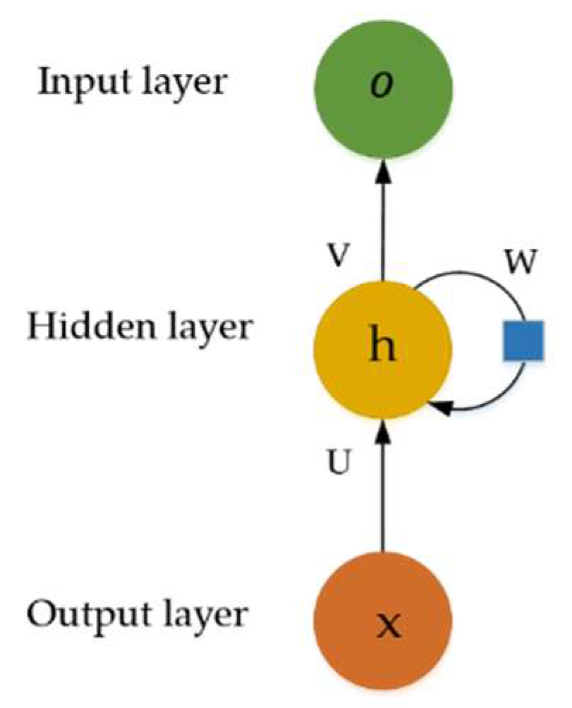
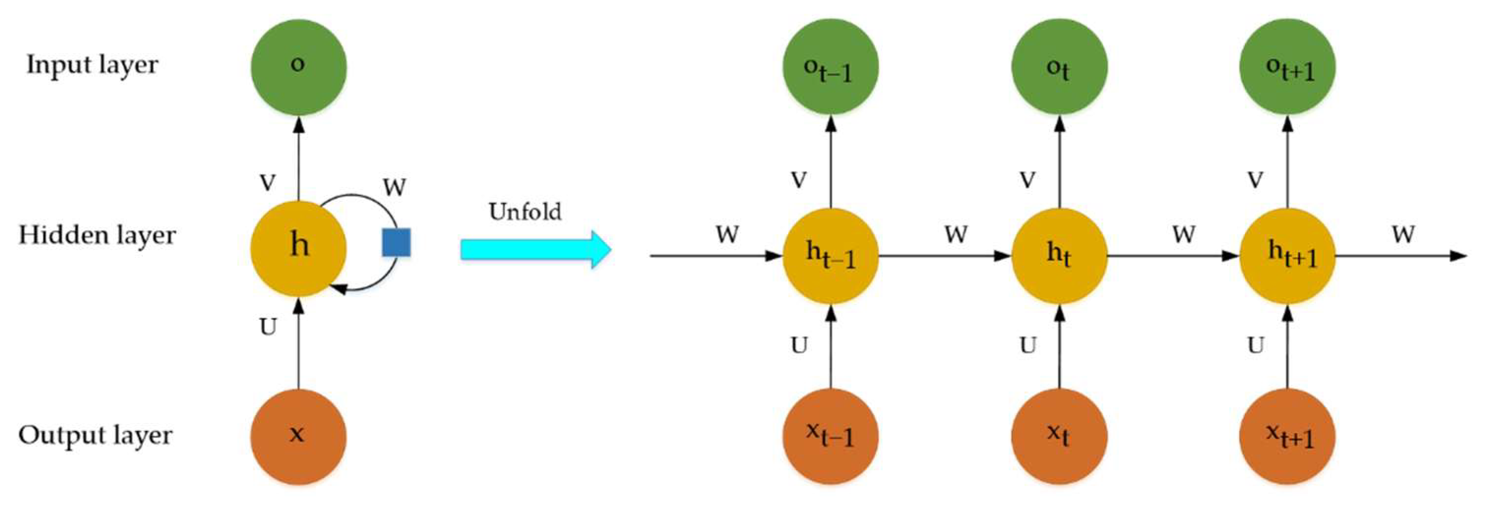
The reflector itself is a complex mechanical structure (as shown in Figure 1), and there are complex nonlinear functional relationships between multiple dimensional parameters of the reflector and multiple optimization objectives. It is necessary to establish a prediction model with high prediction accuracy for the optimization objectives of the reflector to complete the optimal design of the reflector. The recurrent neural network (RNN) is suitable for fitting the nonlinear relationship between input and output variables. To improve the generalization ability of the recurrent neural network, the Bayesian regularization algorithm can optimize the weights of the recurrent neural network, which improves the generalization ability of the recurrent neural network [18,19,20,
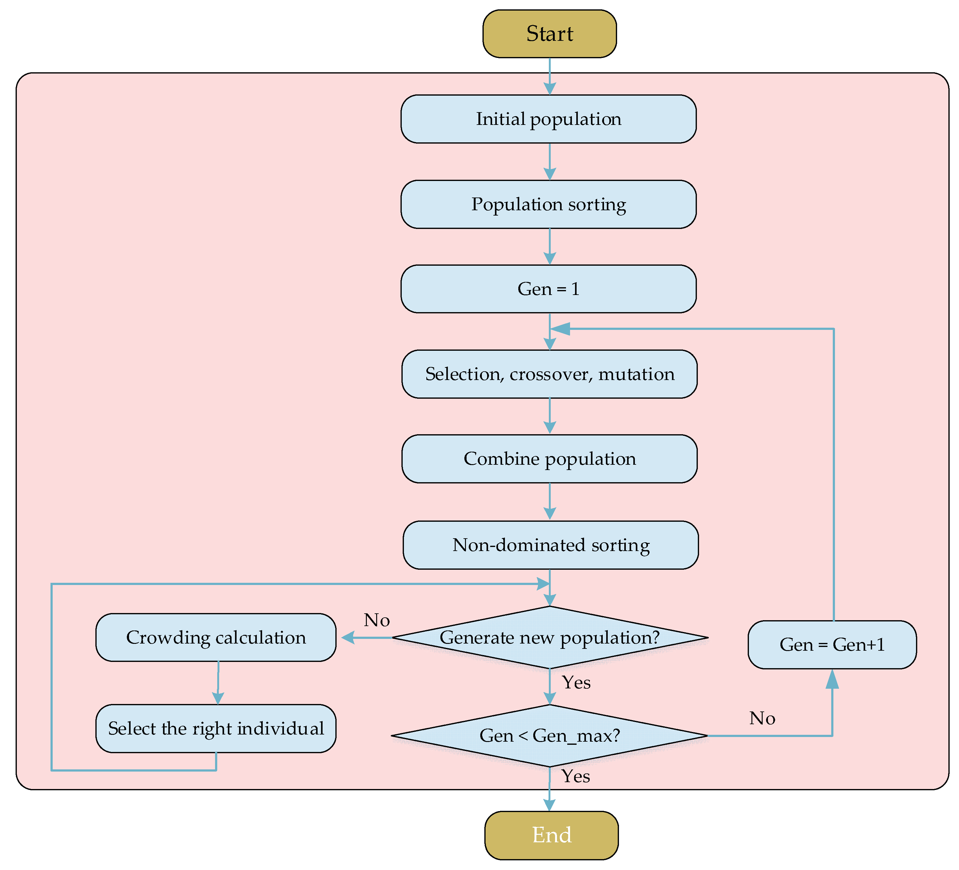
21]. In order to solve the multi-objective optimization problem, Srinivas and Deb proposed the non-dominated sorting genetic algorithm (NSGA) in 1995 [22]. Deb et al. proposed the non-dominated sorting genetic algorithm-II (NSGA-II) in 2000, which improved on the shortcomings of NSGA by adopting the fast non-dominated sorting approach, elitist approach, and parameter-less sharing approach [23]. The NSGA-II method offers advantages of high efficiency and accuracy in solving multi-objective optimization problems [23,24,25]. In this paper, we propose a recurrent neural network based on the Bayesian regularization algorithm and NSGA-II algorithm (BR-RNN-NSGA-II) to complete the optimal design of the reflector. The rest of the paper is organized as follows. Section 2 discusses the theory of the recurrent neural network based on the Bayesian regularization algorithm and the theory of the NSGA-II method. Section 3 builds the prediction model of the optimization objective of the reflector and then completes the multi-objective optimization design using the NSGA-II method. Section 4 takes the reflector of a space camera as an example to complete the optimization design of the reflector and verify the effectiveness of the method proposed in this paper. Section 5 summarizes the research work of this paper and concludes.

2. Fundamental Theory

2.1. RNN

RNN originated in the 1980s and 1990s [26,27,28,29,30,31]. RNN offers a strong nonlinear fitting capability. RNN consists of an input layer, a hidden layer, and an output layer [32], where the value of the hidden layer vector h is determined by the input layer x and the previous moment hidden layer vector h, and the value of the output layer vector o is determined by the hidden layer vector h. Figure 2 illustrates the basic structure of a recurrent neural network. A schematic diagram of the recurrent neural network unfolding in chronological order is shown in Figure 3. The computation process of the recurrent neural network from the input layer to the output layer is shown in Equations (1)–(4).
a t   = U   ·   x t + W ·   h t - 1 + b
where a t denotes the input matrix of the hidden layer at time t, U denotes the weight matrix from the input layer to the hidden layer,   x t denotes the input layer vector at time t, W denotes the weight matrix from the hidden layer to the hidden layer, h t - 1 denotes the output vector of the hidden layer at moment t − 1, and b denotes the bias matrix from the input layer to the hidden layer.
h t   = f ( a t )
where h t denotes the output vector of the hidden layer at time t and f(·) denotes the activation function from the input layer to the hidden layer.
c t   = V   · h t + d
where c t denotes the input matrix of the output layer, V denotes the weight matrix of the hidden layer to the output layer, and d denotes the bias matrix of the output layer.
o t   = g ( c t )
where o t denotes the output vector of the output layer at time t, and g(·) denotes the activation function from the hidden layer to the output layer.

2.2. BR

The loss function of RNN uses the mean squared difference function, as shown in Equation (5). The Bayesian regularization algorithm [33] improves the generalization ability of the RNN by adjusting the objective function of the RNN [34,35,36] so that the RNN avoids overfitting. The loss function of RNN after the adjustment of the Bayesian regularization algorithm is shown in Equation (6) [37,38].
E r =   1 m i = 1 m ( y i o i ) 2
where E r denotes the loss function of the RNN, m denotes the number of samples, y i denotes the actual output of the ith sample, and o i denotes the predicted output of the ith sample.
E u   =   α · E r +   β ·   E p
where E u denotes the adjusted objective function, E p denotes the squared and mean values of each element in the weight matrix, and α and β denote the regularization parameters.

2.3. NSGA-II

Deb et al. proposed the NSGA method to solve multi-objective optimization problems [22], and it has been widely used in many problems. NSGA features disadvantages, such as high computational complexity, lack of elite strategy, and the need to set shared parameters. Therefore, Deb et al. proposed NSGA-II, which made some improvements to NSGA and overcame its disadvantages [23]. NSGA-II computational process mainly includes the processes of population selection, crossover, variation, merging, non-dominated ranking, and crowding degree calculation. The computational flow of NSGA-II is shown in Figure 4.

2.4. BR-RNN-NSGA-II

The structure of the reflector is complex, and it needs to optimize the multi-objective optimal design of multiple reflector design indexes by combining multiple dimensional parameters of itself. This paper proposes BR-RNN-NSGA-II to solve the reflector optimization design problem. BR-RNN-NSGA-II can be divided into two steps. In the first step, an RNN method based on the Bayesian regularization algorithm is used to train the training samples to obtain a high-precision prediction model of reflector design indexes. In the second step, NSGA-II is used to optimize the design of the main mirror indexes with multiple objectives to obtain the best optimization results. BR-RNN-NSGA-II offers the following advantages: (1) BR-RNN-NSGA-II can fit the nonlinear functional relationship between the input and output variables of the reflector well; (2) the reflector design indexes established by BR-RNN-NSGA-II offers high prediction accuracy; (3) BR-RNN-NSGA-II avoids a large number of finite element calculations by establishing the prediction model of reflector design indexes, which improves the optimization design efficiency and reduces the time cost; (4) the introduction of the Bayesian regularization algorithm can improve the generalization ability of RNN and avoid the phenomenon of RNN overfitting; (5) NSGA-II offers the advantages of low computational complexity and low accuracy of optimization results, low complexity, high accuracy of optimization results, and keeping the diversity of populations. NSGA-II is very suitable for solving multi-objective optimization problems.

3. Optimal Design Model of Reflector

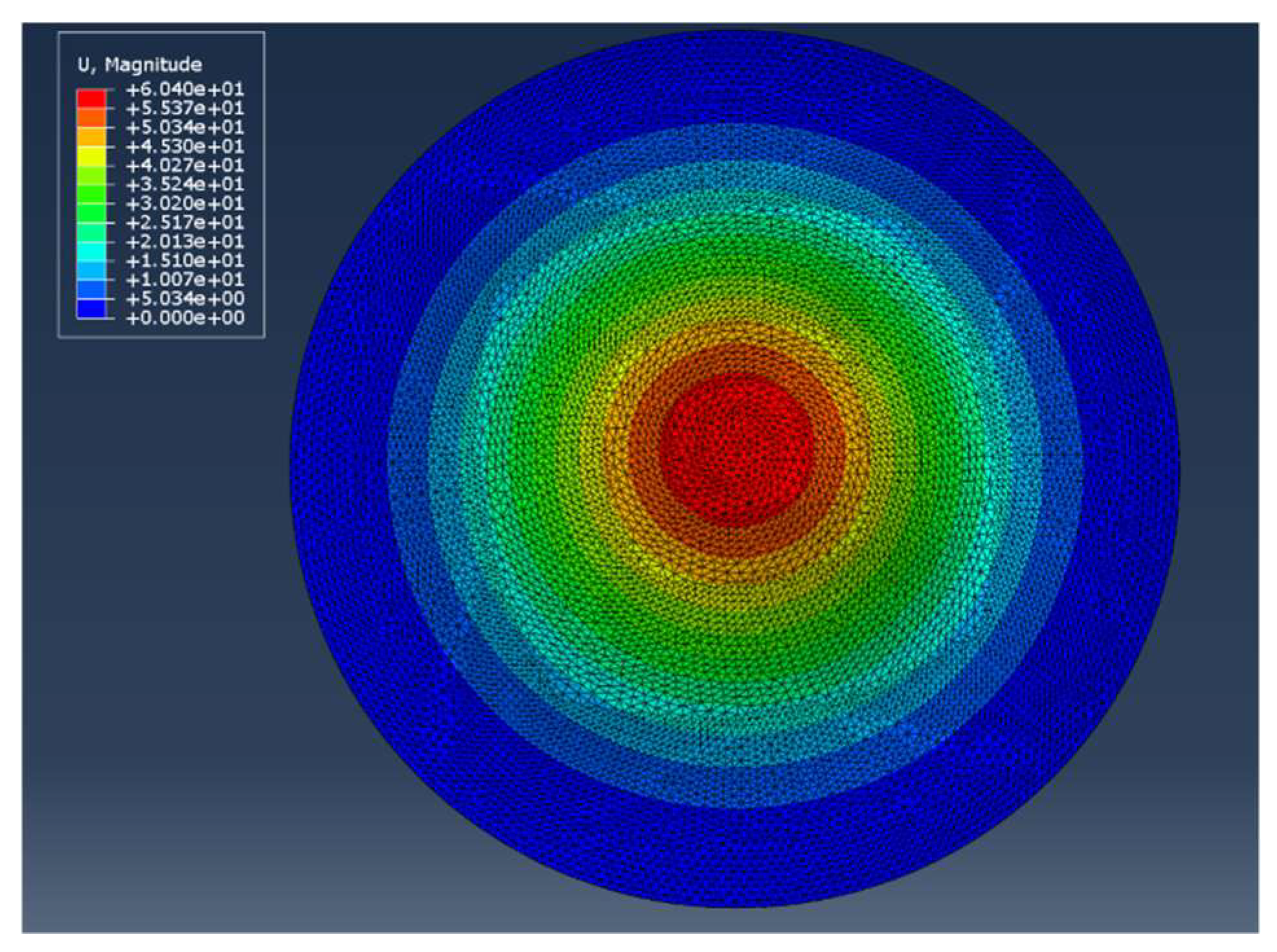
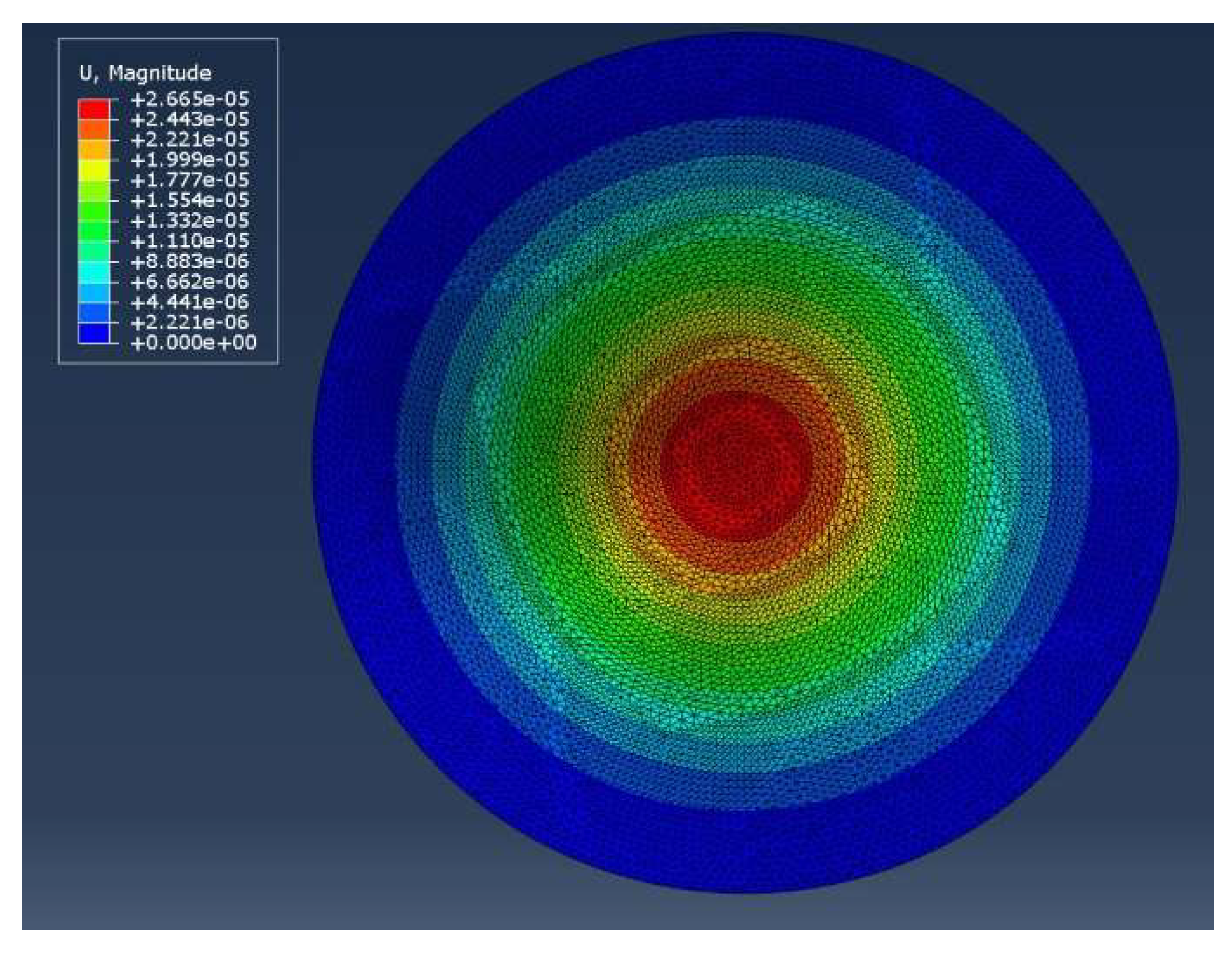
During the ground fabrication and test phase, the reflector image quality is affected by the influence of gravity. In order to avoid resonance of the reflector during the launch, it is necessary to ensure that the reflector features a certain stiffness to resist external interference. In order to reduce the launch cost, the mass of the mirror needs to be reduced as much as possible. In summary, the root mean square value of gravitational mirror deformation root mean square (GMDRMS) is selected to characterize the effect of gravity on the imaging quality of the mirror, the first-order modal frequency (FMF) of the mirror is selected to characterize the stiffness of the mirror, and mass is selected to characterize the mass of the mirror. This paper uses GMDRMS, FMF, and mass as the optimization objectives of the reflector.

3.1. Obtain Sample Data for the Reflector

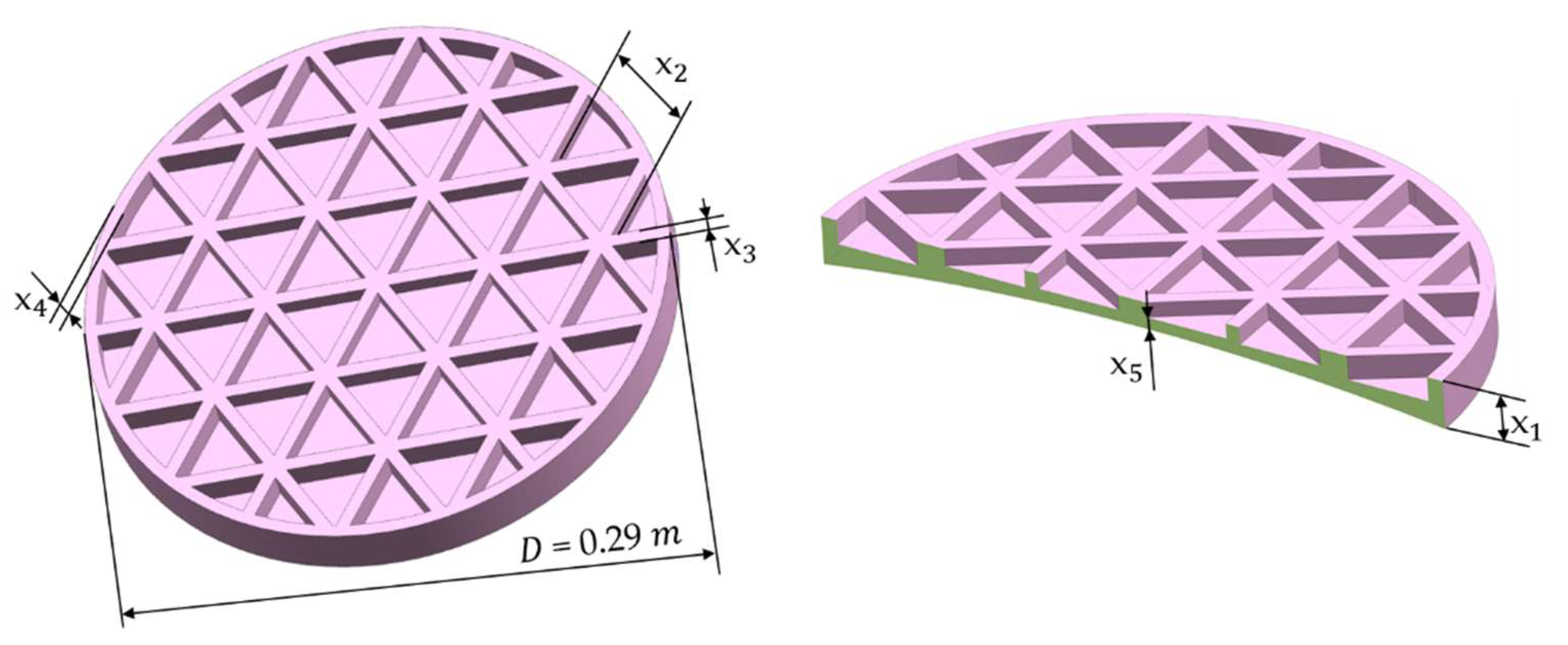
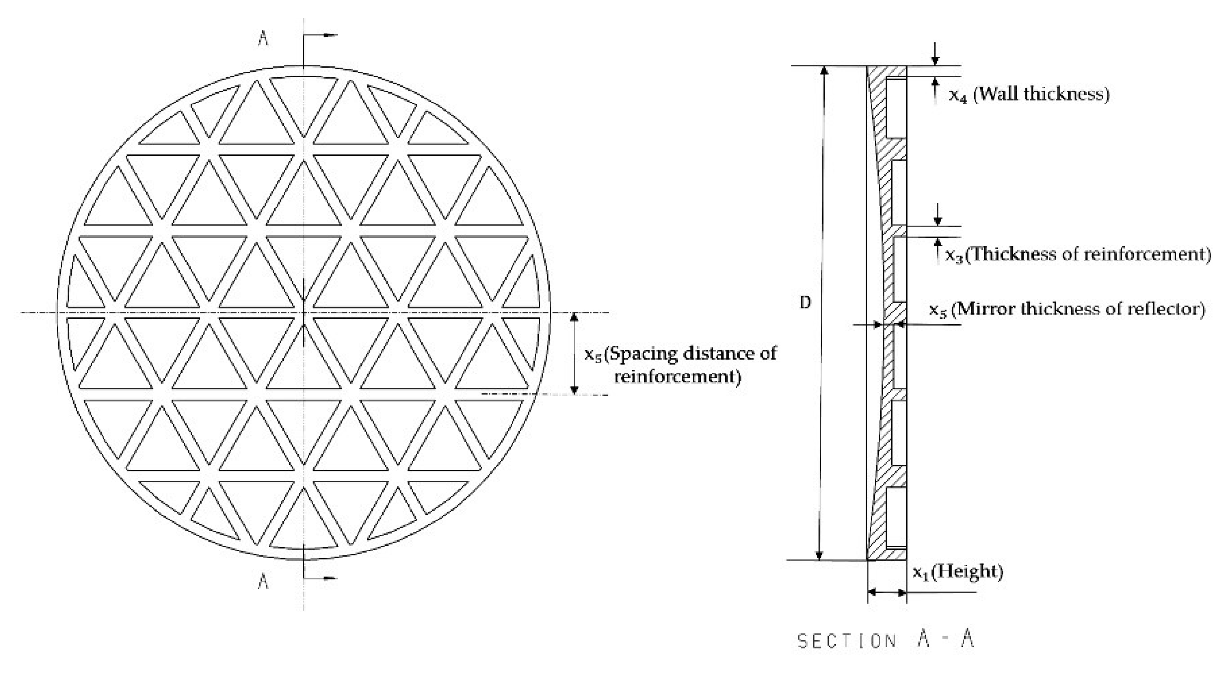
The shape of the lightweight hole at the back of the reflector are triangular, quadrilateral, hexagonal, circular and scalloped. The triangular hole was chosen for this paper because of its high stability compared to other shaped holes. There are five dimension parameters to be optimized for the reflector, which are the height of the reflector (x1), the spacing distance of the reinforcement (x2), the thickness of the reinforcement (x3), the wall thickness of the outer ring of the reflector (x4) and the minimum thickness of the mirror surface of the reflector (x5). The schematic diagram of the reflector structure is shown in Figure 5.
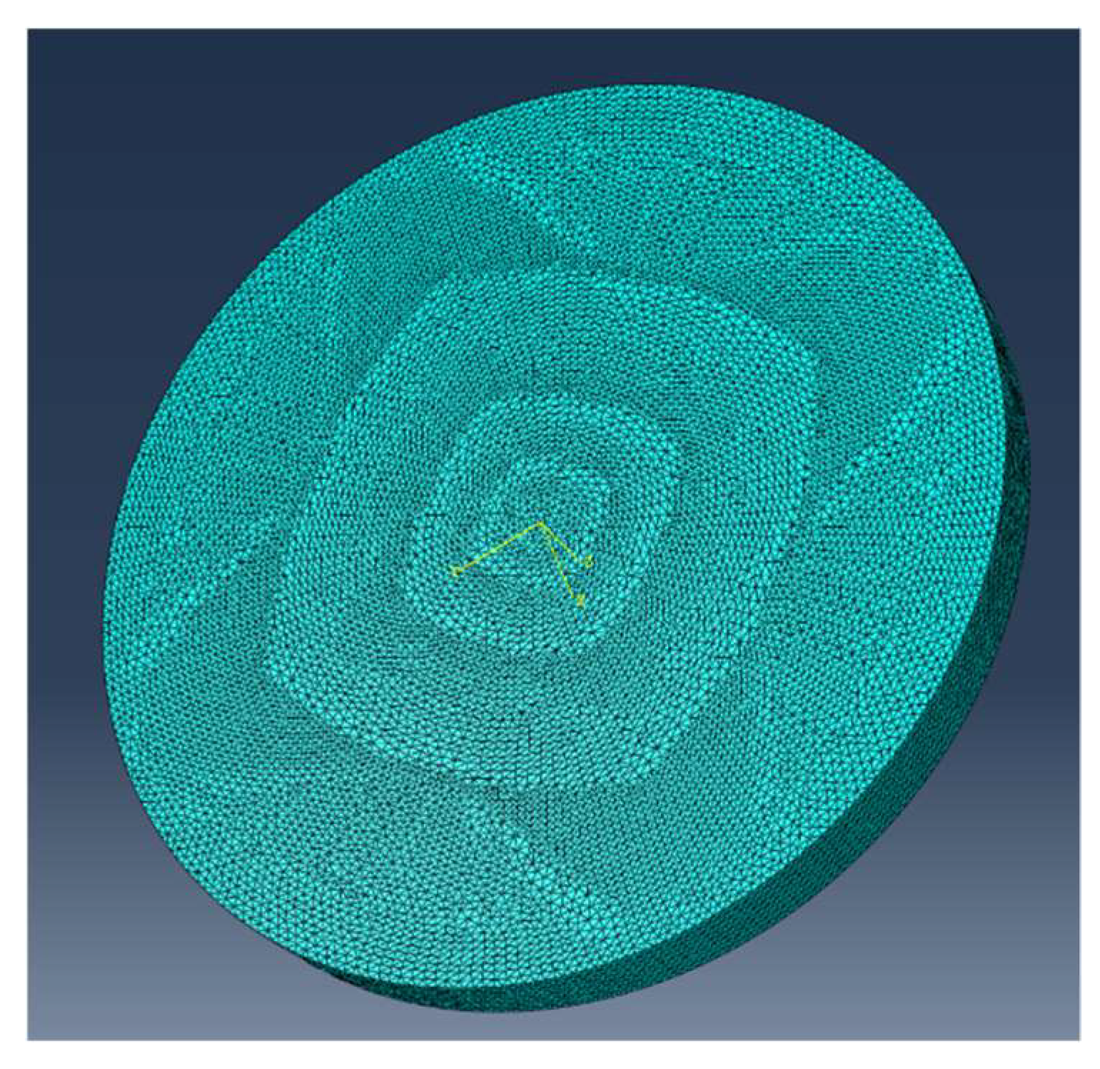
Firstly, five-dimension parameters of the reflector are extracted to build a parametric 3D model. Secondly, the GMDRMS, FMF, and mass of the reflector are calculated by the finite element method. The schematic diagram of the reflector after dividing the grid is shown in Figure 6. Thirdly, the Latin square sampling is used to sample the dimensional parameters of the reflector to obtain several sets of sample input data. Finally, an integrated analysis platform is built to calculate the output data corresponding to each set of sample data of the reflector separately.

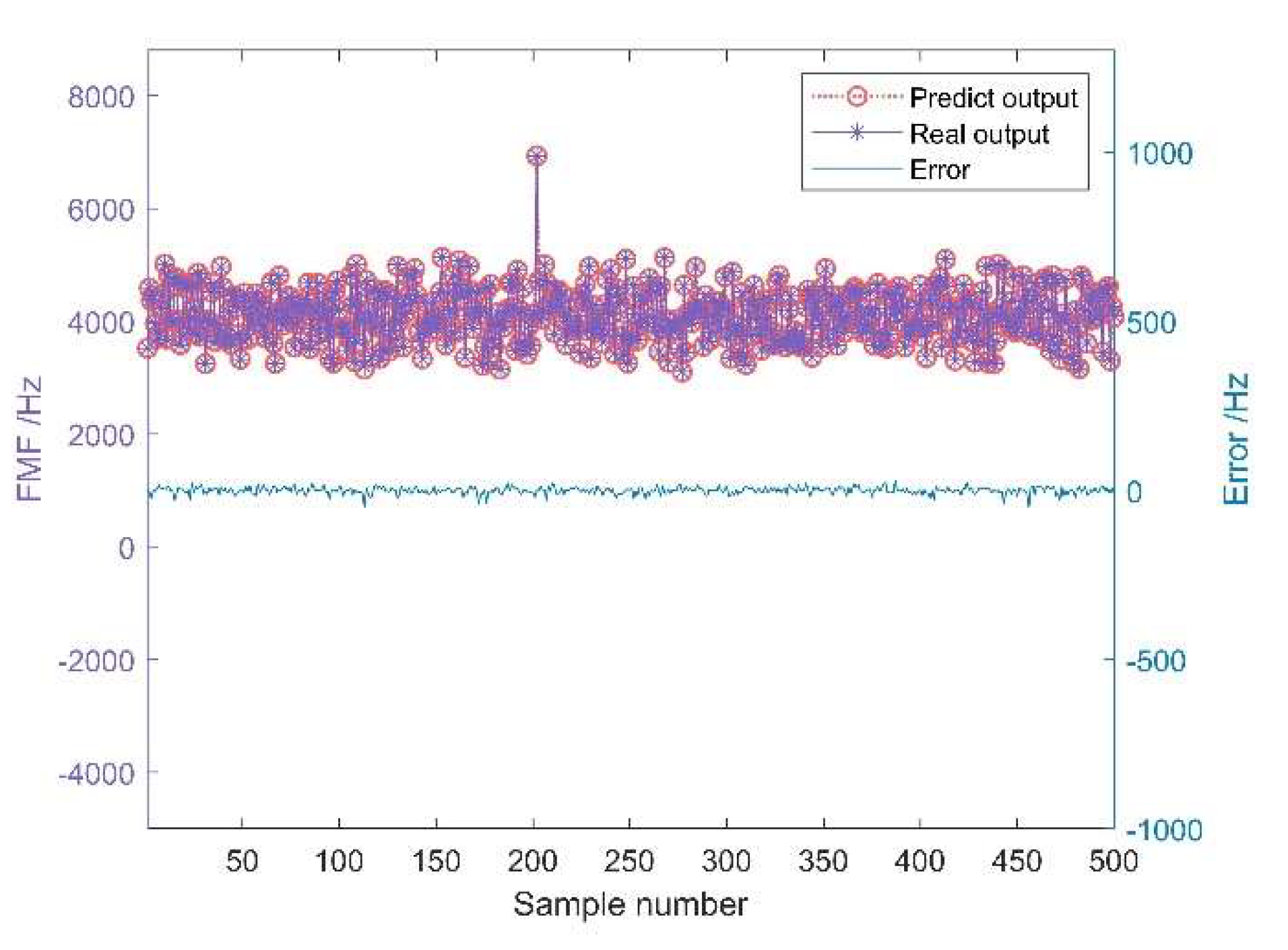
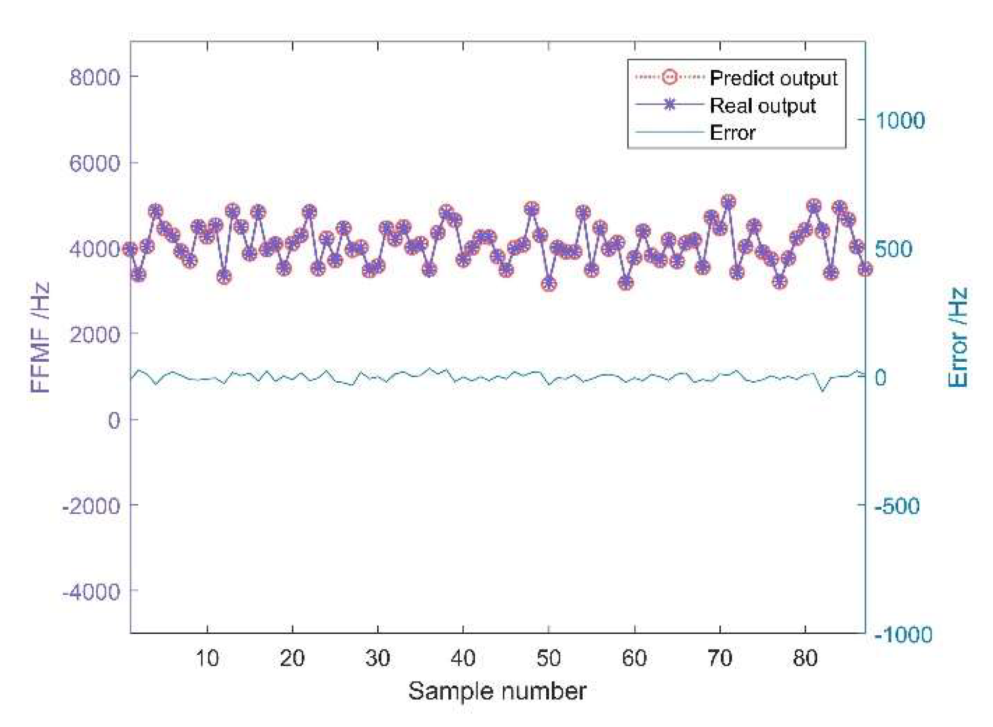
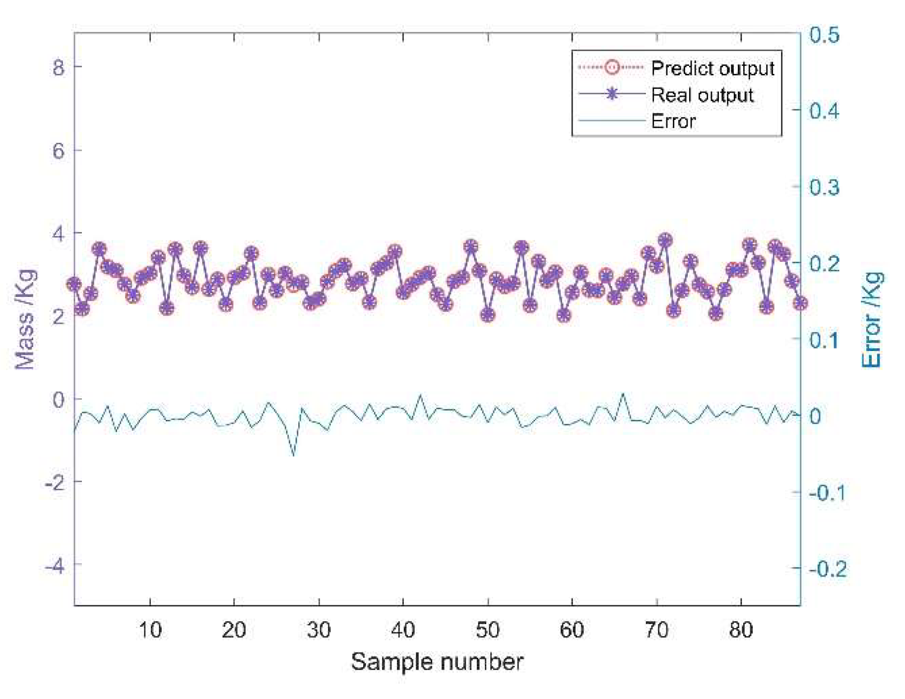
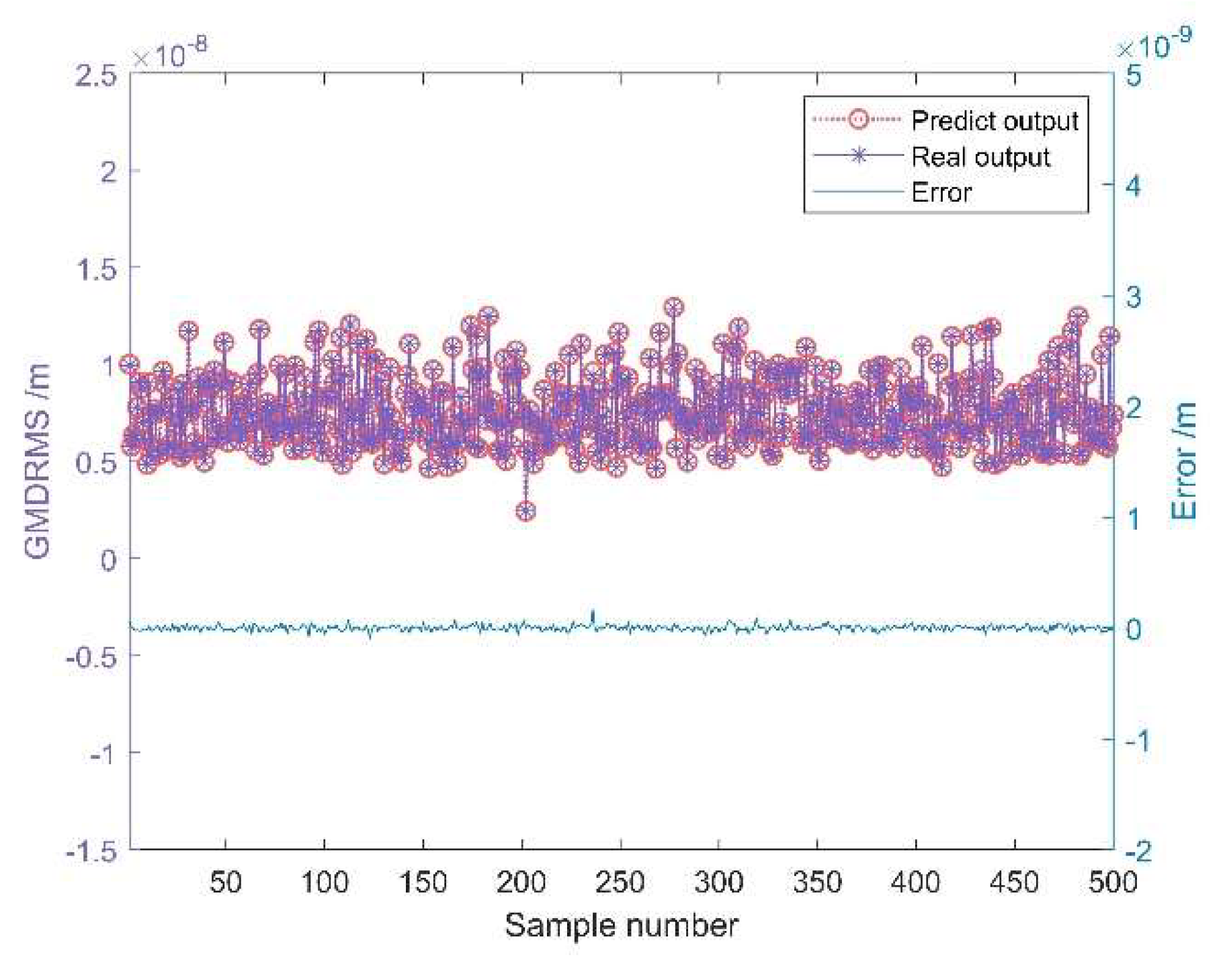
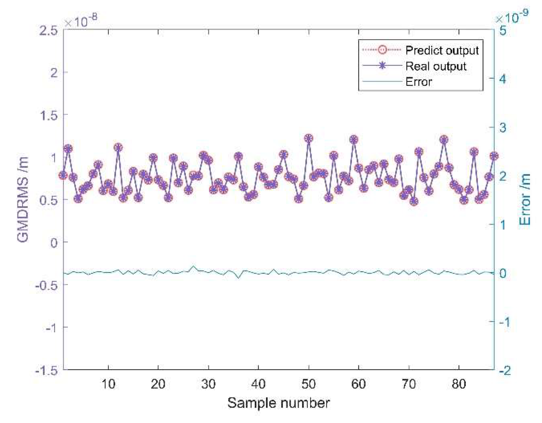
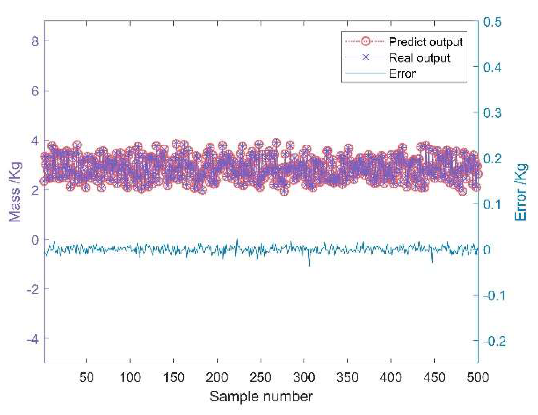
3.2. Develop a Prediction Model for the Reflector Design Indexes

First, the sample data obtained in part 3.1 are randomly divided into training and test sets according to a certain ratio. Next, the training set is trained using the first step in BR-RNN-NSGA-II and validated with the test set to obtain a reflector design indexes prediction model with high prediction accuracy.

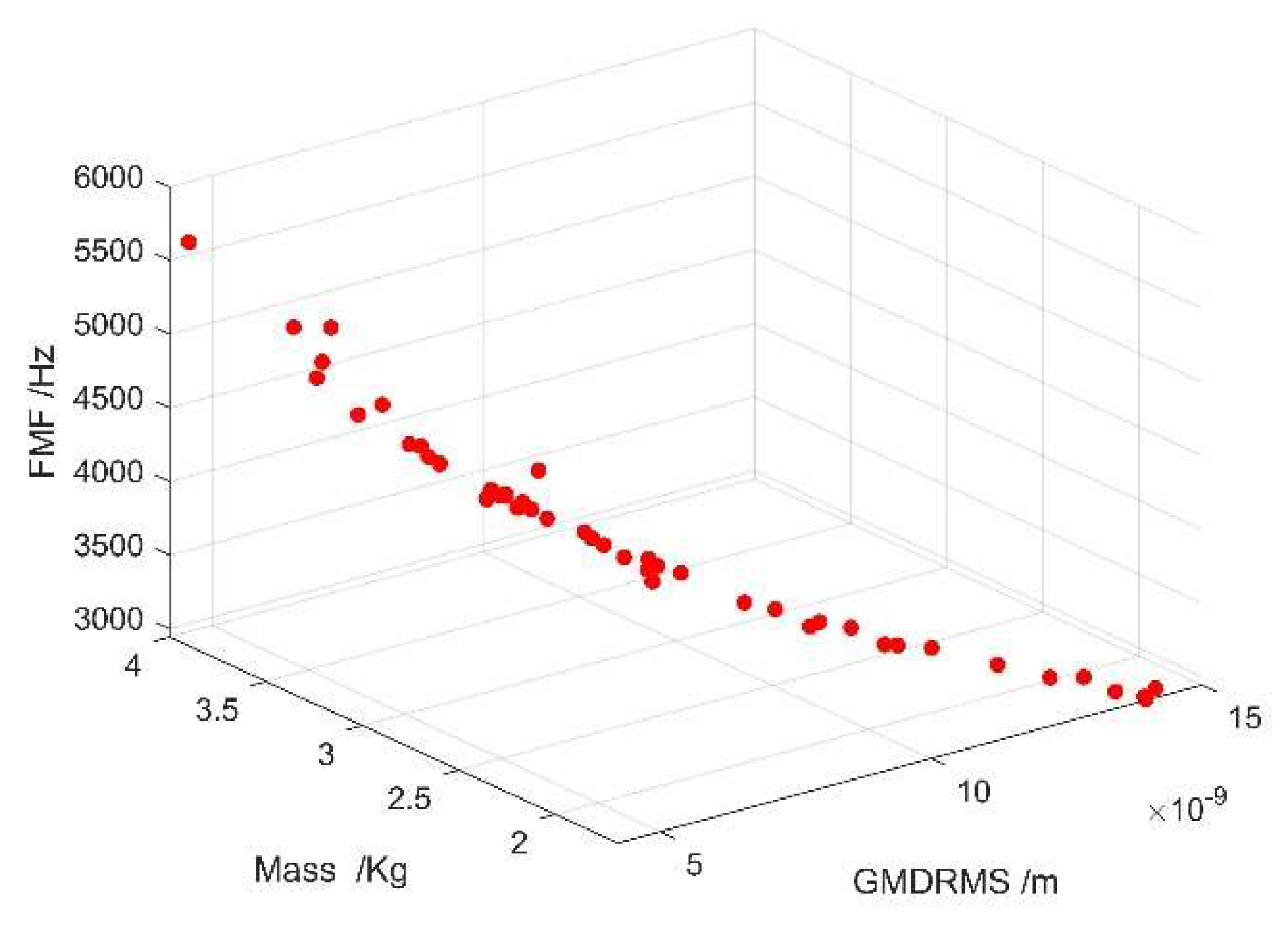
3.3. Multi-Objective Optimization of the Reflector

First, the optimization objective of the reflector and the parameters to be optimized are determined. Next, the boundary conditions and other constraints of the parameters to be optimized are set. Finally, the second step of BR-RNN-NSGA-II is used to perform the global optimization of the reflector design indexes and obtain the best optimization results.

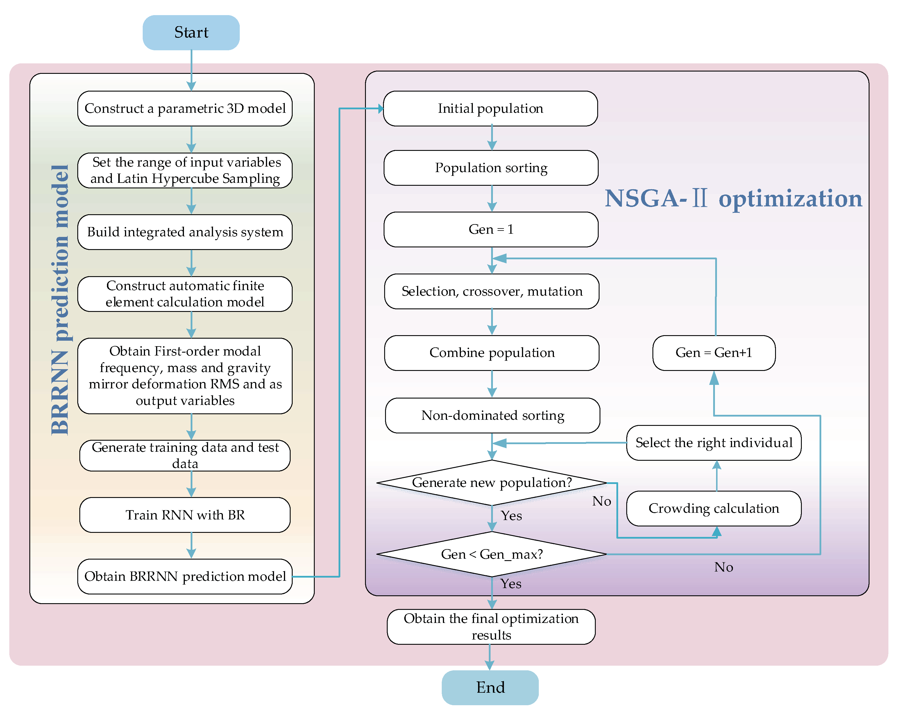
3.4. Reflector Optimization Design Flow Chart

The flow chart of the optimized design of the reflector is shown in Figure 7.

4. An Example of a Reflector

The reflector is an important part of the optical structure of the space camera, and it is necessary to optimize the design of the reflector to meet the requirements of imaging quality, stiffness, and light weight. BR-RNN-NSGA-II ensures that the reflector meets the design requirements by optimizing the dimensional parameters of the reflector.

4.1. Preliminary Work for Reflector

The shape of the lightweight hole at the back of the reflector is adopted as a triangle, and SiC is chosen as the reflector material. The finite element model of the reflector was established using the parametric method. The design indexes of reflector are affected by many independent dimensional parameters, which include the height of the reflector (x1), the spacing distance of the reinforcement (x2), the thickness of the reinforcement (x3), the wall thickness of the outer ring of the reflector (x4) and the minimum mirror thickness of the reflector (x5). The functional relationship between the input random variables and the output response is shown in Equation (7)–(9).
F ( x ) = f ( x 1 , x 2 , x 3 , x 4 , x 5 )
G ( x ) = g ( x 1 , x 2 , x 3 , x 4 , x 5 )
M ( x ) = m ( x 1 , x 2 , x 3 , x 4 , x 5 )
where F ( x ) denotes the objective function of the first-order modal frequency, G ( x ) denotes the objective function of the root mean square value of the gravitational specular deformation and M ( x ) denotes the objective function of the mass.

4.2. Reflector Integration Analysis

The integrated analysis technique is mainly used to automate the process of performing simulation calculations by interfacing the data flow between different design software, which can save a significant amount of labor costs. In the process of obtaining samples for the reflector, 587 sets of input data are first sampled by the Latin hypercube sampling method for the five dimension parameters. Next, then the integrated analysis technique is used to obtain the FMF and mass values for each set of samples. Finally, the GMDRMS values are obtained by gravity field analysis for each set of samples. The cloud diagram of the first-order modal frequency of the reflector and the cloud diagram of the gravity mirror deformation are shown in Figure 8 and Figure 9. Through the above steps, 587 sets of sample data of the reflector regarding the input variables and output response can be reflected. The range of dimensional parameter variations of the reflector mirror is shown in Table 1.

4.3. Build the Design Indexes Prediction Model

First, the 587 sets of sample data of the reflector were randomly divided into 500 sets as the training set and the remaining 87 sets as the test set. Next, the training set was trained by BR-RNN-NSGA-II and validated with the data from the test set to obtain the prediction model of the reflector design indexes. The comparative effects of the prediction model on the predicted and real values of GMDRMS are shown in Figure 10 and Figure 11. The results of the indexes for evaluating the prediction model on the prediction effect of GMDRMS are shown in Table 2. The evaluation indexes of the prediction model include mean absolute error (MAE), mean squared error (MSE), mean square root error (RMSE), and mean prediction accuracy (MPA).
Similarly, the comparison effects of the predicted and real values of the prediction model on FMF are shown in Figure 12 and Figure 13, and the results of the indexes for evaluating the prediction effect of the prediction model on FMF are shown in Table 3. The comparative effects of the prediction model on the predicted and real values of mass are shown in Figure 14 and Figure 15, and the results of the indexes for evaluating the prediction effect of the prediction model on mass are shown in Table 4.

4.4. Reflector Optimization

In order to ensure that the reflector is resistant to external interference, the reflector needs to feature a certain degree of stiffness. The mass of the reflector needs to be as small as possible in order to reduce the emission cost. In addition, the G ( x ) of the mirror needs to be as small as possible. The mathematical model for the multi-objective optimal design of the reflector is as follows.
Find   x = ( x 1 , x 2 , x 3 , x 4 , x 5 ) T
min F ( x ) ,   G ( x ) ,   M ( x )
s . t . { 16   ×   10 3   m     x 1     25   ×   10 3   m 20   ×   10 3   m     x 2     70   ×   10 3   m 3   ×   10 3   m     x 3     10   ×   10 3   m 5   ×   10 3   m     x 4     15   ×   10 3   m 5   ×   10 3   m     x 5     20   ×   10 3   m
BR-RNN-NSGA-II is used to analyze the above mathematical model and obtain optimal Pareto front solution sets, as shown in Figure 16. Combining with the actual requirements of the project, the set that satisfies G(x) ≤ λ/40 (λ = 6.32 × 10⁻⁷ m) and F ( x ) ≥ 3000 Hz with the minimum M ( x ) is selected from the Pareto front solution set as the final optimization result. The design solutions that meet the practical requirements are given in Table 5.

4.5. Analysis of Optimization Results

The BR-RNN-NSGA-II proposed in this paper predicts the reflector design indexes well. As shown in Figure 10 and Figure 11 and in Table 2, the prediction performance of the training and test sets of GMDRMS is excellent, with a mean absolute error of 2.02 × 10⁻¹¹ m and 2.91 × 10⁻¹¹ m, mean squared error of 7 × 10⁻²² m2 and 1.3 × 10⁻²¹ m2, root mean squared error of 2.65 × 10⁻¹¹ m and 3.67 × 10⁻¹¹ m and mean prediction accuracy of 99.73% and 99.60%, respectively. As shown in Figure 12 and Figure 13 and in Table 3, the prediction performance of the training and test sets of FMF is excellent, with mean absolute errors of 13.13 Hz and 7.77 Hz, mean square error of 109.82 Hz2 and 269.78 Hz2, root mean square errors of 10.48 Hz and 16.42 Hz and mean prediction accuracy of 99.81% and 99.68%, respectively. As shown in Figure 14 and Figure 15 and in Table 4, the prediction performance of the training and test sets of mass is excellent, with mean absolute error of 5.8 × 10⁻³ Kg and 9.5 × 10⁻³ Kg, mean square error of 5.5 × 10⁻⁵ Kg2 and 1.4 × 10⁻⁴ Kg2, root mean square error of 7.4 × 10⁻³ Kg and 1.2 × 10⁻³ Kg and mean prediction accuracy of 99.79% and 99.66%, respectively. The mean prediction accuracy of both the training and test sets of GMDRMS, FMF and mass is high, avoiding the overfitting phenomenon.
The mean prediction accuracy of the reflector design indexes prediction model established in this paper was compared with other methods, as shown in Table 6. By comparing the methods in Table 6, we found that the prediction performance of BR-RNN-NSGA-II is better than other methods.
The results of the multi-objective optimal design of reflector by BR-RNN-NSGA-II proposed in this paper are shown in Figure 16. BR-RNN-NSGA-II can complete multi-objective optimization search efficiently and accurately, and we can see the distribution of the optimal solution set, so as to provide a reference for the final selection of the design solution. In addition, the comparison of the results and time spent between BR-RNN-NSGA-II and the Monte Carlo method is shown in Table 7, which shows that BR-RNN-NSGA-II outperforms the Monte Carlo method in terms of GMDRMS, FMF, mass and time spent. Compared with [13,15], BR-RNN-NSGA-II offers higher prediction accuracy and better search efficiency.

5. Conclusions

This paper proposes BR-RNN-NSGA-II to optimize the design of the reflector structure and verifies the effectiveness of the method by an example. The work reported in this paper is summarized as follows.
(1)
BR-RNN-NSGA-II uses the RNN method to fit the nonlinear function between the dimensional parameters of the reflector structure and the design indexes.
(2)
BR-RNN-NSGA-II incorporates the BR algorithm into the RNN method, which can improve the generalization ability of the RNN method and avoid the phenomenon of overfitting.
(3)
By comparing with other methods, BR-RNN-NSGA-II offers the highest mean prediction accuracy of 99.60% or more for the reflector design indexes.
(4)
BR-RNN-NSGA-II applies NSGA-II to optimize the multi-objective design of multiple design indexes of the reflector efficiently and accurately.
(5)
BR-RNN-NSGA-II saves a significant amount of finite element calculation time and improves the optimization efficiency by optimizing the design of the reflector.
This paper provides an applicable method for the optimal design of space camera mirrors. In this paper, BR-RNN-NSGA-II is proposed for the optimal design of reflector design indexes. BR-RNN-NSGA-II features high prediction accuracy, strong generalization ability and efficient multi-objective optimization, which can avoid a large number of finite element calculations. It is hoped that BR-RNN-NSGA-II can play a significant role in the optimal design of reflectors for large-aperture multi-physical field analysis. In the future, the influence of changes in reflector geometry parameters on the performance of optical system will be explored in depth.

Author Contributions

Conceptualization, X.Z. and L.S.; methodology, L.Q.; software, X.Z.; validation, L.Q., and L.S.; formal analysis, X.Z.; data curation, X.Z.; writing—original draft preparation, X.Z.; writing—review and editing, X.Z., L.S. and L.Q. All authors have read and agreed to the published version of the manuscript.

Funding

This research received no external funding.

Conflicts of Interest

The authors declare no conflict of interest.

References

  1. Liu, S.; Hu, R.; Li, Q.; Zhou, P.; Dong, Z.; Kang, R. Topology optimization-based lightweight primary mirror design of a large-aperture space telescope. Appl. Opt. 2014, 53, 8318–8325. [Google Scholar] [CrossRef]
  2. Liu, F.; Li, W.; Zhao, W.; Zhao, H.; Lin, G.; Wang, X. Topology Optimization Based Parametric Design of Balloon Borne Telescope’s Primary Mirror. Appl. Sci. 2021, 11, 5077. [Google Scholar] [CrossRef]
  3. Qu, Y.; Jiang, Y.; Feng, L.; Li, X.; Liu, B.; Wang, W. Lightweight Design of Multi-Objective Topology for a Large-Aperture Space Mirror. Appl. Sci. 2018, 8, 2259. [Google Scholar] [CrossRef] [Green Version]
  4. Shao, M.Q.; Lei, Z.; Jia, X. Opto-mechanical integrated optimization of a lightweight mirror for space camera. Appl. Opt. 2020, 60, 539–546. [Google Scholar] [CrossRef] [PubMed]
  5. Liu, G.; Guo, L.; Wang, X.; Wu, Q. Topology and parametric optimization based lightweight design of a space reflective mirror. Opt. Eng. 2018, 57, 075101. [Google Scholar] [CrossRef]
  6. Li, Z.; Chen, X.; Wang, S.; Jin, G. Optimal design of a Φ760 mm lightweight SiC mirror and the flexural mount for a space telescope. Rev. Sci. Instrum. 2017, 88, 125107. [Google Scholar] [CrossRef] [PubMed]
  7. Wang, Q.; Chen, J.; Wang, J.; You, Y.; Sun, J.; Wu, S. Structural Optimization of Composite Wind Turbine Blade under Aerodynamic Loads. J. Mech. Eng. 2014, 50, 114–121. [Google Scholar] [CrossRef]
  8. Jansen, P.W.; Perez, R.E. Constrained structural design optimization via a parallel augmented Lagrangian particle swarm optimization approach. Comput. Struct. 2011, 89, 1352–1366. [Google Scholar] [CrossRef]
  9. Rosso, M.M.; Cucuzza, R.; Trapani, F.D.; Marano, G.C. Nonpenalty Machine Learning Constraint Handling Using PSO-SVM for Structural Optimization. Adv. Civ. Eng. 2021, 2021, 6617750. [Google Scholar] [CrossRef]
  10. Sun, W.; Cao, W.; Gu, Y. Research on Antenna Cabin Structure Optimization Based on Response Surface and Multi-island Genetic Algorithm. IOP Conf. Ser. Mater. Sci. Eng. 2019, 575, 012018. [Google Scholar] [CrossRef]
  11. Belarhzal, S.; Boudi, E.M. Genetic Algorithm Design Optimization for Non-Standard Spur Gears. In Digital Technologies and Applications; Springer: Cham, Switzerland, 2021. [Google Scholar]
  12. Shan, X.Y.; Wang, B.C.; Xu, K.K.; Li, H.X. Surrogate Model Based Structure Optimization of Jetting System. IEEE Trans. Compon. Packag. Manuf. Technol. 2020, 10, 494–501. [Google Scholar] [CrossRef]
  13. Kihm, H.; Yang, H.-S. Design optimization of a 1-m lightweight mirror for a space telescope. Opt. Eng. 2013, 52, 091806. [Google Scholar] [CrossRef]
  14. Wang, S.; Li, J.; Zhang, F.; Qi, G. Optimization of large aperture space reflector based on RSM. Infrared Laser Eng. 2013, 42, 291–297. [Google Scholar]
  15. Qin, T.; Guo, J.; Jing, Z.; Han, P.; Qi, B. Hybrid IPSO-IAGA-BPNN algorithm-based rapid multi-objective optimization of a fully parameterized spaceborne primary mirror. Appl. Opt. 2021, 60, 3031–3043. [Google Scholar] [CrossRef] [PubMed]
  16. Wang, D.; Zhang, S.; Tan, F.; Zhi, X.; Zhen, R. A Method on Lightweight for the Primary Mirror of Large Space-Based Telescope Based on Neural Network. In Proceedings of the International Symposium on Optoelectronic Technology & Application: Imaging Spectroscopy & Telescopes & Large Optics, Beijing, China, 13–15 May 2014. [Google Scholar]
  17. Ye, W.; Dong, J. Optimized design of lightweight structural parameters for large-aperture primary mirror. Chin. Opt. 2012, 5, 222–228. [Google Scholar]
  18. Tian, L.; Noore, A. Software reliability prediction using recurrent neural network with bayesian regularization. Int. J. Neural Syst. 2004, 14, 165–174. [Google Scholar] [CrossRef]
  19. Li, G.; Li, B.-J.; Yu, X.-G.; Cheng, C.-T. Echo State Network with Bayesian Regularization for Forecasting Short-Term Power Production of Small Hydropower Plants. Energies 2015, 8, 12228–12241. [Google Scholar] [CrossRef] [Green Version]
  20. Liang, Y. Gene Expression Temporal Patterns Classification with Hierarchical Bayesian Neural Networks and Time Lagged Recurrent Neural Networks. Ph.D. Thesis, The University of Memphis, Memphis, TN, USA, 2003. [Google Scholar]
  21. Perez-Ramirez, C.A.; Amezquita-Sanchez, J.P.; Valtierra-Rodriguez, M.; Adeli, H.; Dominguez-Gonzalez, A.; Romero-Troncoso, R.J. Recurrent neural network model with Bayesian training and mutual information for response prediction of large buildings. Eng. Struct. 2019, 178, 603–615. [Google Scholar] [CrossRef]
  22. Srinivas, N.; Deb, K. Multiobjective Function Optimization Using Nondominated Sorting Genetic Algorithms. Evol. Comput. 1995, 2, 1301–1308. [Google Scholar]
  23. Deb, K.; Agrawal, S.; Pratap, A.; Meyarivan, T. A Fast Elitist Non-Dominated Sorting Genetic Algorithm for Multi-Objective Optimization: NSGA-II. In International Conference on Parallel Problem Solving from Nature; Springer: Berlin/Heidelberg, Germany, 2000. [Google Scholar]
  24. Zhao, Z.; Liu, B.; Zhang, C.; Liu, H. An improved adaptive NSGA-II with multi-population algorithm. Appl. Intell. 2018, 49, 569–580. [Google Scholar] [CrossRef]
  25. Yuan, M.; Li, Y.; Zhang, L.; Pei, F. Research on intelligent workshop resource scheduling method based on improved NSGA-II algorithm. Robot. Comput.-Integr. Manuf. 2021, 71, 102141. [Google Scholar] [CrossRef]
  26. Jordan, M.I. Serial Order: A Parallel Distributed Processing Approach; AD-A-173989/5/XAB; ICS-8604; Institute for Cognitive Science University of California: San Diego, CA, USA, March 1986. [Google Scholar]
  27. Elman, J.L. Finding Structure in Time. Cogn. Sci. 1990, 14, 179–211. [Google Scholar] [CrossRef]
  28. Hochreiter, S.; Schmidhuber, J. Long short-term memory. Neural Comput. 1997, 9, 1735–1780. [Google Scholar] [CrossRef] [PubMed]
  29. Schuster, M.; Paliwal, K.K. Bidirectional recurrent neural networks. IEEE Trans. Signal Process. 1997, 45, 2673–2681. [Google Scholar] [CrossRef] [Green Version]
  30. Hopfield, J.J. Neural networks and physical systems with emergent collective computational abilities. Proc. Natl. Acad. Sci. USA 1982, 79, 2554–2558. [Google Scholar] [CrossRef] [Green Version]
  31. Werbos, P.J. Backpropagation through time: What it does and how to do it. Proc IEEE 1990, 78, 1550–1560. [Google Scholar] [CrossRef] [Green Version]
  32. Graves, A. Supervised Sequence Labelling with Recurrent Neural Networks (Studies in Computational Intelligence #385); Springer: Berlin/Heidelberg, Germany, 2012. [Google Scholar]
  33. MacKay, D.J.C. Bayesian Interpolation. Neural Comput. 1992, 4, 415–447. [Google Scholar] [CrossRef]
  34. Foresee, F.D.; Hagan, M.T. Gauss-Newton approximation to Bayesian learning. In Proceedings of the International Conference on Neural Networks (ICNN’97), Houston, TX, USA, 12 June 1997; pp. 1930–1935. [Google Scholar]
  35. Cawley, G.C.; Talbot, N.L.C. Preventing Over-Fitting during Model Selection via Bayesian Regularisation of the Hyper-Parameters. J. Mach. Learn. Res. 2007, 8, 841–861. [Google Scholar]
  36. Hagan, M.T.; Demuth, H.B.; Beale, M.H. Neural Network Design; PWS Publishing Co.: Boston, MA, USA, 1996. [Google Scholar]
  37. Yang, B.; Li, D.; Zeng, C.; Chen, Y.; Guo, Z.; Wang, J.; Shu, H.; Yu, T.; Zhu, J. Parameter Extraction of PEMFC via Bayesian Regularization Neural Network based Meta-heuristic Algorithms. Energy 2021, 228, 120592. [Google Scholar] [CrossRef]
  38. Atyabi, S.A.; Afshari, E. Three-dimensional multiphase model of proton exchange membrane fuel cell with Honeycomb flow field at the cathode side. J. Clean. Prod. 2019, 214, 738–748. [Google Scholar] [CrossRef]
Figure 1. Schematic diagram of the structure of the reflector.
Machines 10 00063 g001
Figure 2. RNN model structure.
Machines 10 00063 g002
Figure 3. A schematic diagram of RNN unfolding in chronological order.
Machines 10 00063 g003
Figure 4. NSGA-II calculation process.
Machines 10 00063 g004
Figure 5. Reflector structure diagram.
Machines 10 00063 g005
Figure 6. Schematic diagram of the reflector grid.
Machines 10 00063 g006
Figure 7. Reflector optimization design process.
Machines 10 00063 g007
Figure 8. Cloud diagram of the first-order modal frequency of the reflector.
Machines 10 00063 g008
Figure 9. Cloud diagram of gravity mirror deformation.
Machines 10 00063 g009
Figure 10. The comparison of the results of the GMDRMS training set.
Machines 10 00063 g010
Figure 11. The comparison of the results of the GMDRMS test set.
Machines 10 00063 g011
Figure 12. The comparison of the results of the FMF training set.
Machines 10 00063 g012
Figure 13. The comparison of the results of the FMF test set.
Machines 10 00063 g013
Figure 14. The comparison of the results of the Mass training set.
Machines 10 00063 g014
Figure 15. The comparison of the results of the Mass test set.
Machines 10 00063 g015
Figure 16. The Pareto frontier solution set optimized by BR-RNN-NSGA-II.
Machines 10 00063 g016
Table 1. The range of variation of the dimensional parameters of the reflector.
Random VariablesMax, 10−3 mMin, 10−3 m
x 1 2516
x 2 7020
x 3 103
x 4 155
x 5 205
Table 2. Evaluation of the predictive effect of GMDRMS.
Evaluation IndicatorsMAE, 10−9 mMSE, 10−18 m2RMSE, 10−9 mMPA
Training samples0.02020.00070.026599.73%
Test samples0.02910.00130.036799.60%
Table 3. Evaluation of the predictive effect of FMF.
Evaluation IndicatorsMAE, HzMSE, Hz2RMSE, HzMPA
Training samples13.13109.8210.4899.81%
Test samples7.77269.7816.4299.68%
Table 4. Evaluation of the predictive effect of mass.
Evaluation IndicatorsMAE, KgMSE, Kg2RMSE, KgMPA
Training samples0.00585.5 × 10−50.007499.79%
Test samples0.00951.4 × 10−40.001299.66%
Table 5. Final optimized design results.
x 1 , m. x 2 , m x 3 ,   m x 4 ,   m x 5 ,   m GMDRMS, mFMF, HzMass, Kg
18.3 × 10−336.5 × 10−33.7 × 10−35.2 × 10−35.0 × 10−31.28 × 10−831421.85
Table 6. MPA comparison of reflector design indexes prediction methods.
MethodsBR-RNN-NSGA-IIGRNNSVMRandom Forest
Training samples of GMDRMS99.73%82.02%98.44%96.04%
Test samples of GMDRMS99.60%81.76%98.46%94.76%
Training samples of FMF99.81%91.61%99.31%98.17%
Test samples of FMF99.68%91.34%99.24%97.35%
Training samples of mass99.79%88.43%99.13%97.74%
Test samples of mass99.66%88.51%99.10%96.96%
Table 7. Comparison of results and time spent between BR-RNN-NSGA-II and Monte Carlo method.
Optimization MethodsGMDRMS, m FMF, HzMass, KgTime Spent/h
Monte Carlo1.29 × 10−831041.9241.09
BR-RNN-NSGA-II1.28 × 10−831421.850.04
Publisher’s Note: MDPI stays neutral with regard to jurisdictional claims in published maps and institutional affiliations.

