4.1. Comparison between Experimental and Numerical Results at 100% Load
A comparison of the results with experimental data can be carried out focusing attention only on the discharge temperature of the combustion chamber. The values reported in
Table 6 refer to nominal conditions for the gas turbine and Standard conditions (ISO) for the environment and summarize the results that have been obtained in terms of pollutant emissions, too. Their concentration represent volume-weighted average values at the outlet section of the burner. NO
x and CO formation can be estimated, but there is only one measured value; for further assessment of the prediction capability of the model, several simulations with different air temperatures at the inlet of the compressor were performed in order to carry out a sensitivity analysis.
Table 6.
Comparison between experimental and numerical result at 100% load and ISO conditions.
Table 6.
Comparison between experimental and numerical result at 100% load and ISO conditions.
| Firing Temperature | NOx Pollutant Emission | CO Pollutant Emission |
|---|
| Experimental measurement | Numerical result and percentage error | Experimental measurement (ppm) | Numerical result and percentage error (ppm) (at 15% O2) | Experimental measurement (ppm) | Numerical result and percentage error (ppm) |
|---|
| 1,373 K | 1,420 K | 83.7 | 84.7 | 11.8 | 11.9 |
| | 3.42% | | +1.25% | | +0.82% |
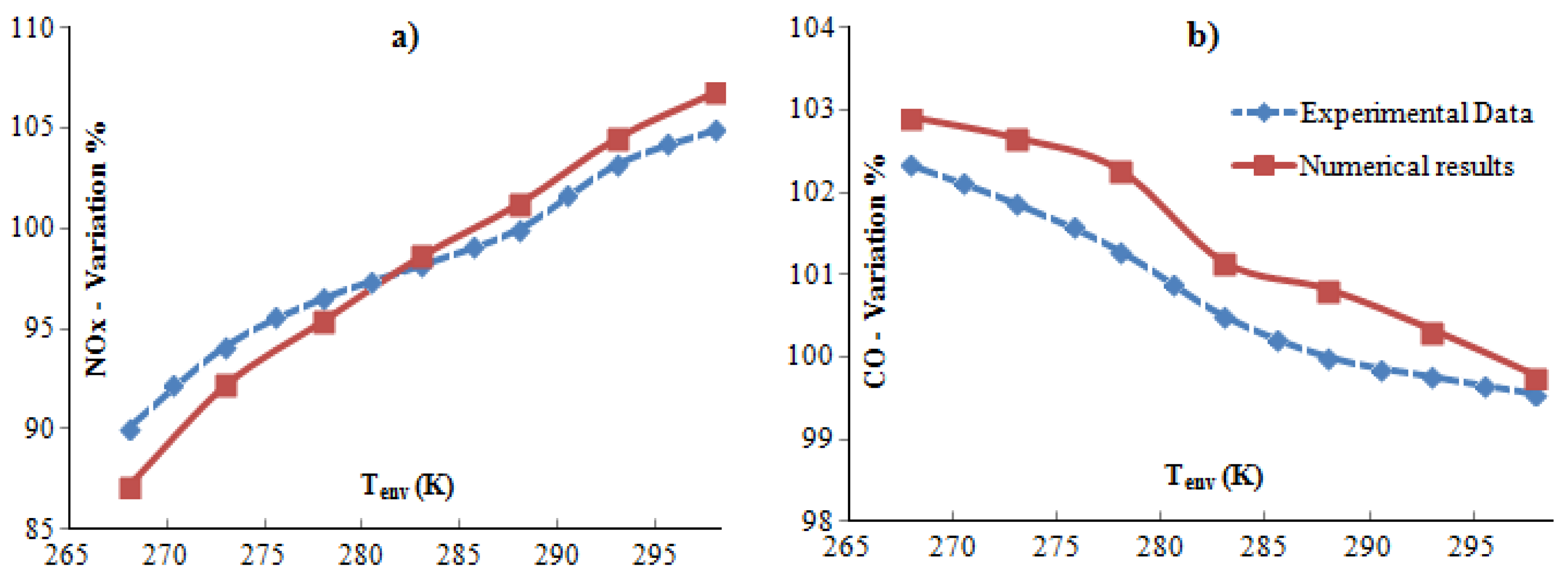
These simulations are also able to examine the response of the gas turbine model to variations in operating condition. In particular, six further simulations have been performed, using inlet temperatures ranging from 268 K to 298 K. In
Table 7, for both experimental and numerical data, the percentages refer to the experimental value reported in
Table 6. The experimental results derive from an averaged process of several experimental conditions close to any operating point taken in consideration. In
Figure 5, other intermediate experimental values have been plotted.
Table 7.
The effect of the air temperature at the compressor inlet on pollutant emissions.
Table 7.
The effect of the air temperature at the compressor inlet on pollutant emissions.
| Air Temperature Inlet (K) | NOx (at 15% O2) | CO |
|---|
| Experimental Value in Comparison with ISO Condition (%) | Numerical Value in Comparison with ISO Condition (%) | Experimental Value in Comparison with ISO Condition (%) | Numerical Value in Comparison with ISO Condition (%) |
|---|
| 268 | 90.05 | 87.15 | 102.33 | 102.91 |
| 273 | 94.16 | 92.22 | 101.87 | 102.66 |
| 278 | 96.54 | 95.41 | 101.29 | 102.27 |
| 283 | 98.19 | 98.63 | 100.50 | 101.15 |
| 288 | 100 | 101.25 | 100 | 100.82 |
| 293 | 103.21 | 104.50 | 99.76 | 100.33 |
| 298 | 104.93 | 106.77 | 99.55 | 99.77 |
Figure 5.
(a) NOx and (b) CO percentage variation for different environmental temperatures.
Figure 5.
(a) NOx and (b) CO percentage variation for different environmental temperatures.
It is evident from the previous figures that the predicted trends are qualitatively similar to the experimental values. In particular, they capture the trend of reduced CO and increased NOx with air temperature rising. As for CO emissions, although the model tends to overestimate the real data, it is evident how the simulations can completely follow the small variations measured on the real machine. In fact, as a typical characteristic of all heavy-duty machine series, the carbon monoxide emissions increase quickly only if the firing temperature is drastically reduced. Therefore, the stability of the numerical model is based on the ability to appreciate these very small variations. However, the methodical overestimation is due to a systematic error in the evaluation of the main parameters of Equation 6. Two different sources of error are the residence time estimation, since UDF elaborates an averaged value, and the numerical temperature at the exit of the burner. Similarly, the supposed pressure loss may deviate from the real value, because there is no experimental data available for its estimation.
To completely evaluate the pollutant emissions, the effect of different mass flow rates of steam injected within the combustion chamber has been studied at full load and ISO condition, also. In a STIG (STeam Injected Gas Turbine) cycle, the amount of injected steam represents a sensible parameter to take into account, since there are practical limits to the amount of steam, as well as water that can be injected into the combustor before a serious flame stability problems occur [
12]. This has been experimentally determined and must be taken into account in all applications if the combustor is to ensure low NO
x emissions and long hardware life for the gas turbine user. In ordinary operating conditions, the steam-to-fuel mass ratio (
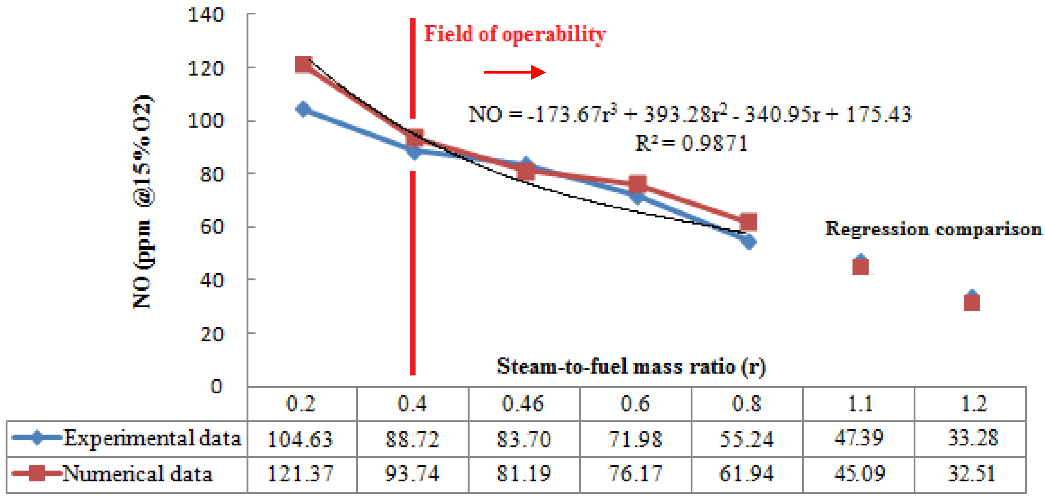
r) is between 0.2 and 0.8. The results shown in
Figure 6 for NO
x have been plotted taking this range as the reference (
r = 0.46 represents the design value).
Figure 6.
NOx emission vs. steam-to-fuel mass ratio.
Figure 6.
NOx emission vs. steam-to-fuel mass ratio.
It is evident how the computational model has a good agreement with experimental results, primarily for intermediate values of r (0.4 ˂ r ˂ 0.6). For values close to the minimum, the code tends to produce a higher percentage of errors at about 15%. These discrepancies could be related to experimental uncertainties in input parameters to the computations that can be amplified in the case of extremely low values of this parameter, producing an overestimation of temperature within the flame zone. If this error cannot be considered tolerable, the field of operability is limited to a steam-to-fuel-mass ratio higher than 0.4; in fact, lower error percentages have been obtained for the other operating conditions within the whole simulated range.
The model analysis has been extended for higher values of r, which are usually adopted just when an increase of electrical power is required. A third order regression curve, built through the numerical data, has been used in the cases of r = 1.1 and r = 1.2. The comparison with experimental data provides an excellent fitting, since very limited differences can be noticed. These results confirm that the software prediction capability can be extended to extremely high values for steam mass flow rate.
The effect of steam injection on CO emission is almost negligible. Steam temperature is very similar to the air temperature, so that experimental data at nominal conditions show no appreciable variations with increasing r. From a numerical point of view, the employed UDF cannot consider the influence of r, because there is no parameter that depends on the steam mass flow rate.
4.1.1. Thermal and Fluid Dynamic Internal Fields
Since the previous study demonstrated the validity of the present CFD model, it is interesting to analyze some physical characteristics of the internal fields of the combustion chamber.
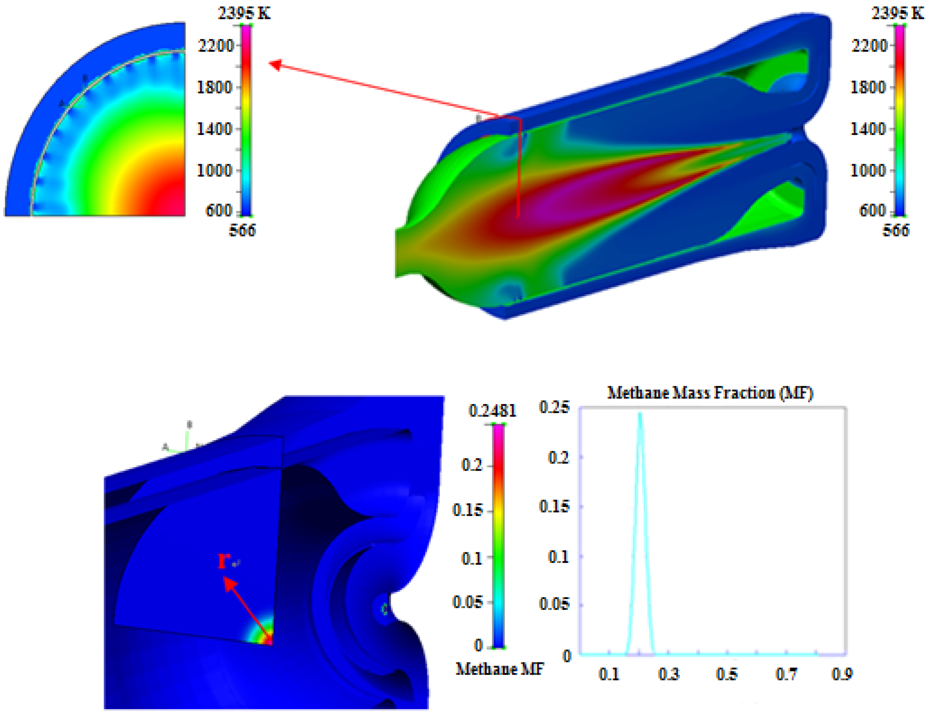
Figure 7a shows the temperature contour plot on the symmetry plane of the burner and on a cutting plane in the dilution zone. Different peculiarities of a non-premixed combustion can be highlighted. First of all, the flame occupies the central and terminal part of the burner, since the chemical species need time for mixing and complete reactions: the primary zone is characterized by the low temperature of the mixture, since the reaction rate is limited by a high mass fraction of the fuel (
Figure 7b).
Figure 7.
(a) Temperature contour plot for a secondary zone cross-section (Left) and the symmetry plane (Right); (b) Methane concentration within the primary zone.
Figure 7.
(a) Temperature contour plot for a secondary zone cross-section (Left) and the symmetry plane (Right); (b) Methane concentration within the primary zone.
Secondly, the flame develops into a thin interface with the air flux and produces a compact body flame: this structure is typical of the diffusive reaction mechanism. The cutting plane on the dilution zone allows one to verify the influence of the cold air flux in preserving walls and decreasing the temperature of exhaust gases before the first stage of the gas turbine.
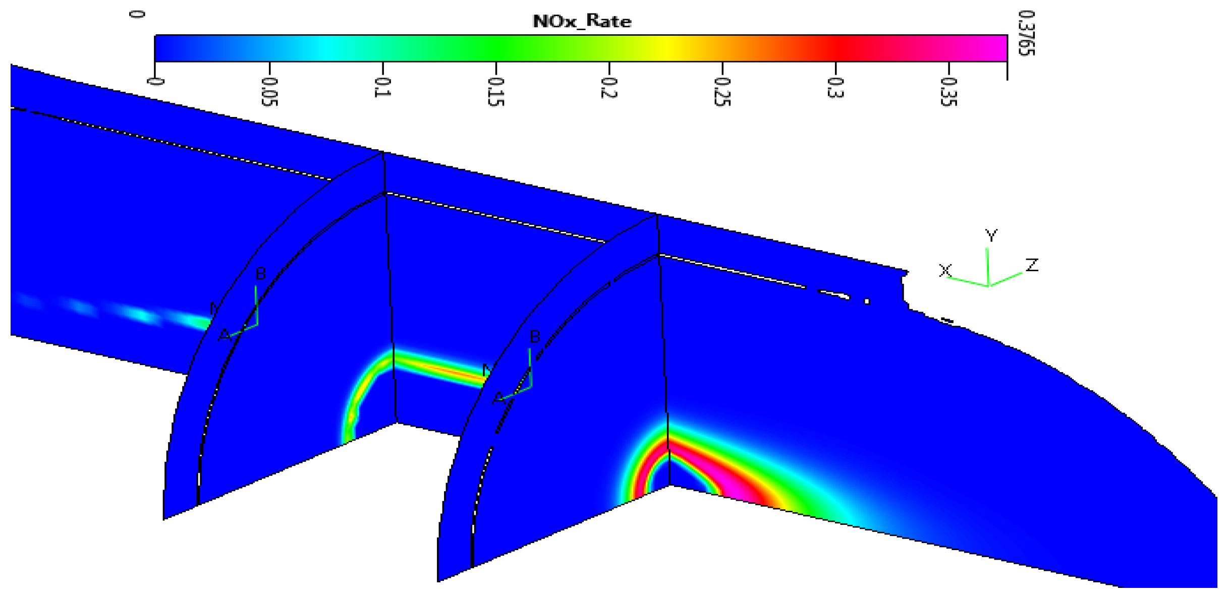
The strong connection between the temperature field and the NO
x production rate is evident in
Figure 8, where three different cross-sections have been plotted. Numerical simulations reveal that the distribution of maximum values follow the flame shape within the secondary zone of the combustion chamber where temperature range exceeds 2,000 K.
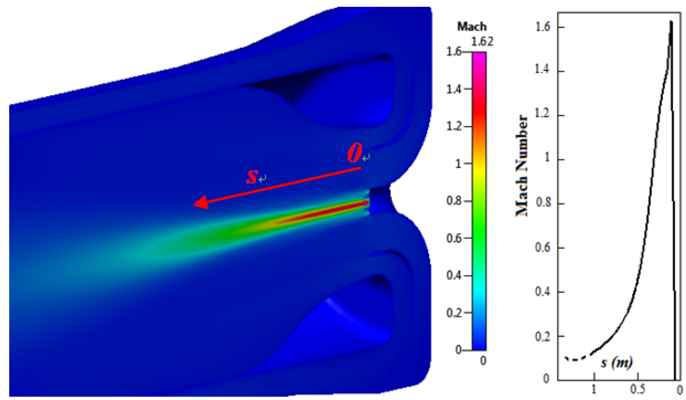
Keeping attention on fluid dynamics, one of the most important parameters that can be verified is the Mach number of the methane jet (
Figure 9). These kind of combustion chambers are not designed to operate with supersonic gaseous jets, and simulations confirm that the injection is characterized by a supersonic flow just near the injectors’ discharge. The delaying action of the air involves a decreasing of the Mach number in the range between 0.5 and 0.8, already within the primary zone.
Figure 8.
NOx production rate on the symmetry plane and on two different normal x cuts.
Figure 8.
NOx production rate on the symmetry plane and on two different normal x cuts.
Figure 9.
Fuel Mach number: contour plot and chart.
Figure 9.
Fuel Mach number: contour plot and chart.
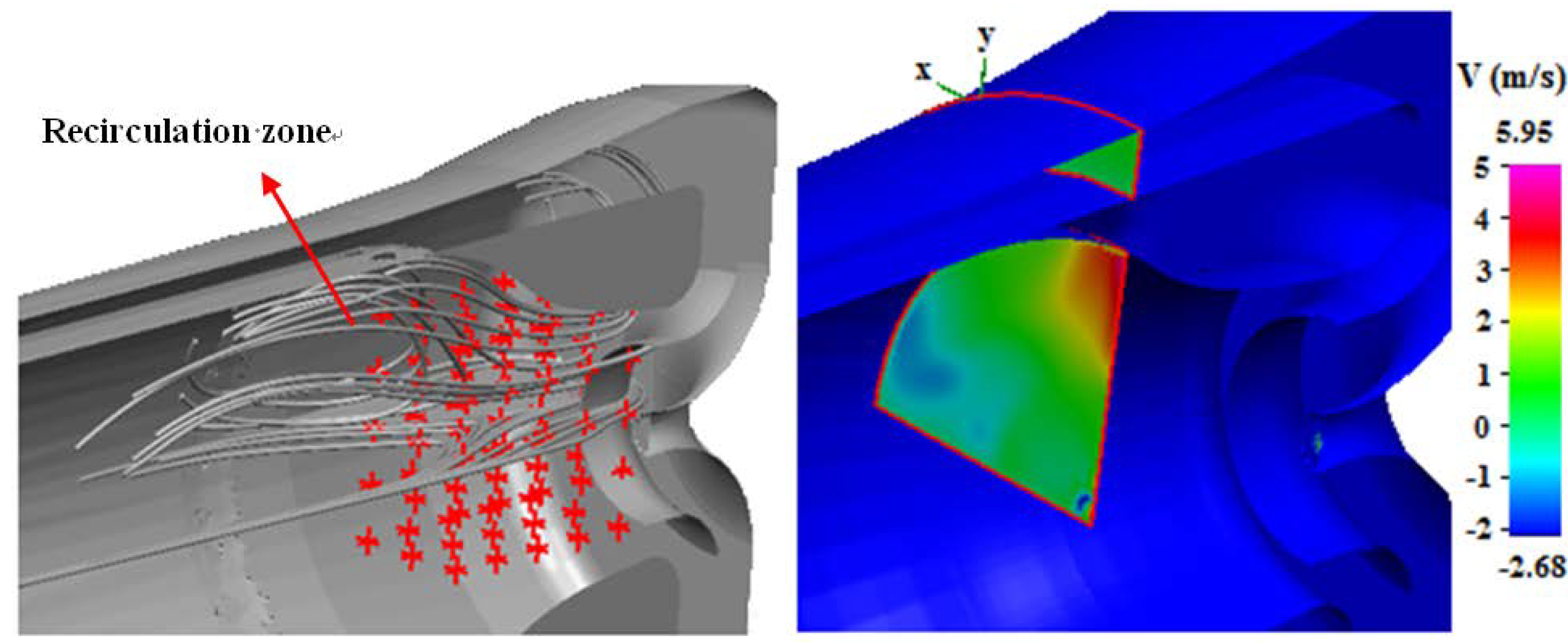
Figure 10 reports the stream lines and the
y-direction velocity contour plot in a cross-section at the beginning of the primary zone. It is evident how the CFD model can describe the recirculation flow at the inlet of the combustion chamber. This is an important phenomenon to take into account, because it influences the pressure losses and the mixing process between reactants.
Figure 10.
Recirculation zone.
Figure 10.
Recirculation zone.
From this point of view, the attention has been focused on the Mach number and recirculation flow to characterize the primary zone, since the employed correlation for CO contains the assessment for Tpz, which is directly influenced by fuel distribution and fluid dynamics. Good results in CO estimation are primarily related to the ability of the model to describe these phenomena.
4.2. Experimental and Numerical Results at Partial Load
As mentioned earlier, the analysis has been extended to 75, 80 and 90% of the nominal thermal power.
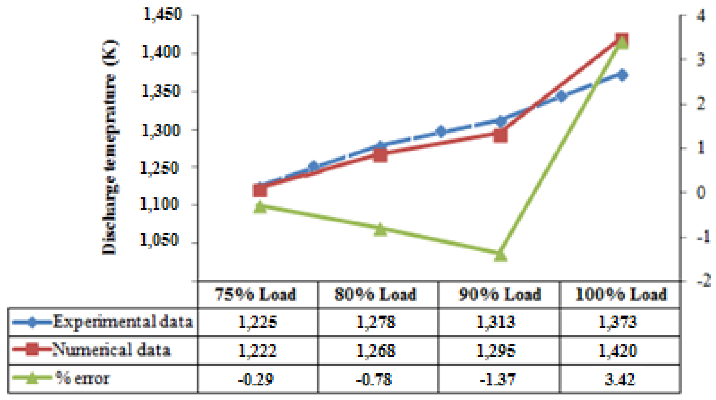
Figure 11 shows the comparison between the computed temperatures and the measured values at the discharge of the combustion chamber. The decreasing trend in temperature is the result of the combination of both the air and fuel lower mass flow rate, due to the (IGV) regulation at the compressor intake. The numerical simulations can provide, in any case, a good agreement with the experimental data, with a maximum value of the error lower than 4%.
Figure 11.
Discharge temperature at different loads.
Figure 11.
Discharge temperature at different loads.
Figure 12 reports the averaged temperature for each cross-section within the intermediary and secondary zones of the combustion chamber: the rough rising in temperature due to the completion of the fuel oxidation is followed by a fast cooling due to the action of the fresh air entering from the dilution zone and the decreasing of the body flame diameter, as can be seen in
Figure 7a. In general, the presence of IGV as a power control system has a slight effect on the NO
x emissions; in fact, the IGV maintains a high exhaust temperature also at partial load conditions, so that the NO
x concentration can vary by a few
ppm.
Figure 12.
Comparison between numerical and experimental temperatures at different load values.
Figure 12.
Comparison between numerical and experimental temperatures at different load values.
However, for the studied cases, the decreasing of the temperature peak reached within the combustion chamber determines a reduction in terms of NO
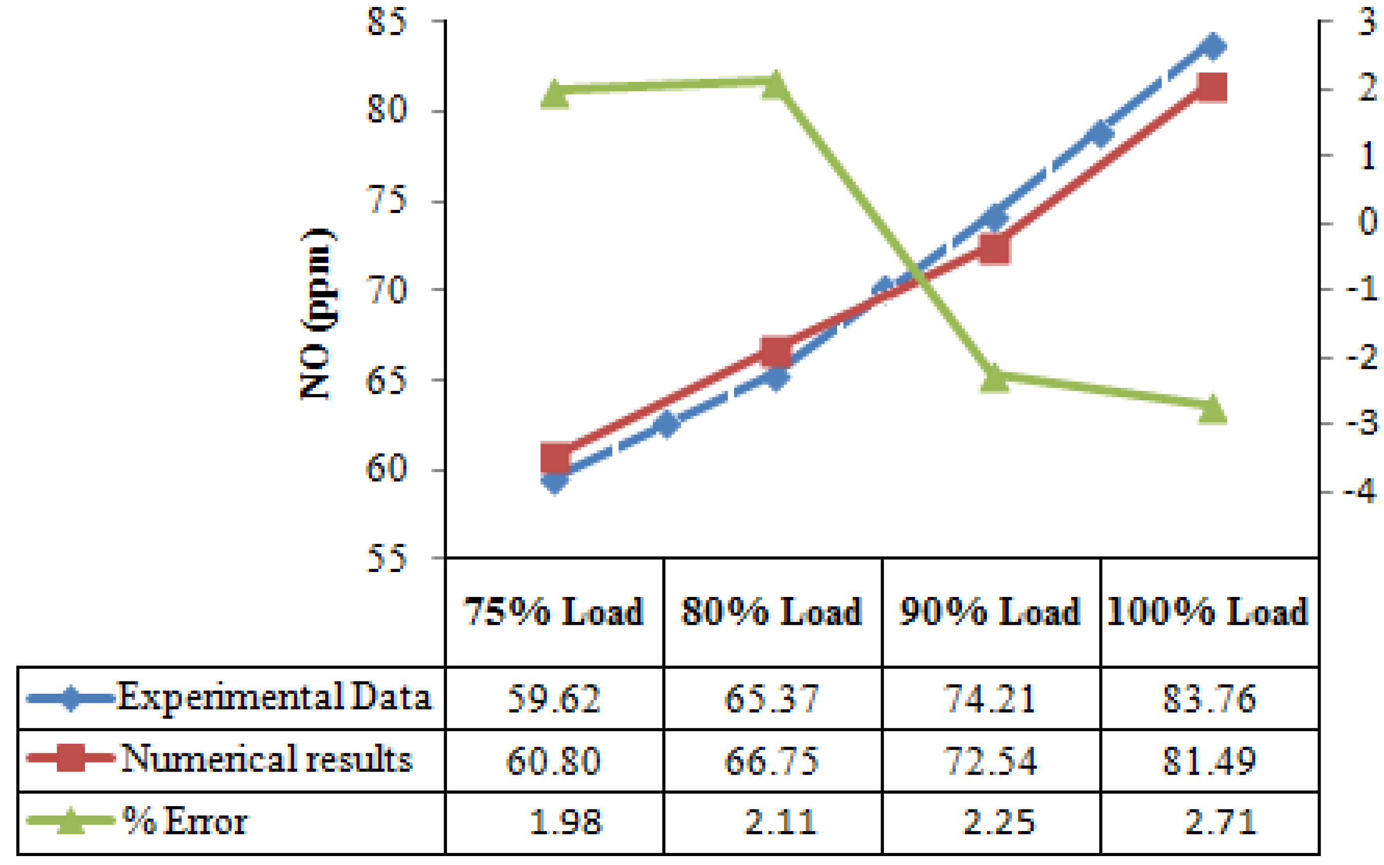
x pollutant emissions. This trend is well described also by the numerical model (
Figure 13): as NO
x strongly depends on temperature, this is an indication that the model can provide an averaged internal thermal field close to the real one.
Figure 13.
NOx prediction at different load values.
Figure 13.
NOx prediction at different load values.
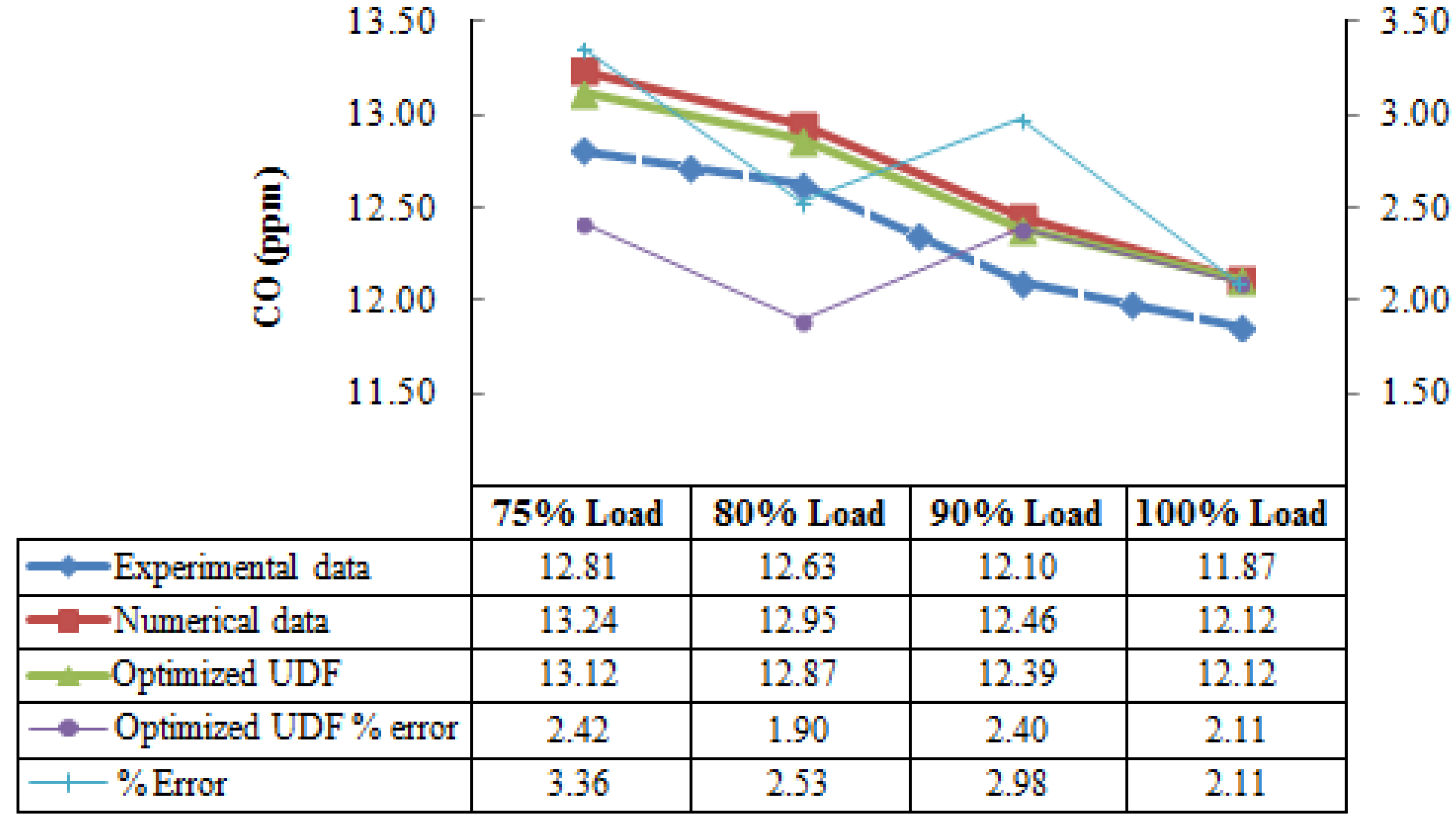
The evaluation of the numerical model performance in terms of CO assessment at partial load has been summarized in
Figure 14. First of all, it is important to underline that the model can predict the increasing in CO emissions, due to the reduction of the peak temperatures within the combustion chamber. However, as well as is seen in the analysis dedicated to the full load condition, also in this case, the software tendency is to overestimate the carbon monoxide concentration at the discharge section of the burner.
Figure 14.
CO prediction at different load values. UDF, user-defined function.
Figure 14.
CO prediction at different load values. UDF, user-defined function.
To improve the UDF and minimize the error, a hybrid strategy can be adopted (
Figure 15): while the numerical temperature, , is directly transferred to the UDF, the experimental value of temperature and experimental CO concentration can be given as the external input. In this way, the code can compute Equation (6) choosing the temperature that minimizes the difference with the experimental value. This approach reduces the error when the estimated temperature is lower than the real one, and it has the advantage of directly joining together the code with real data.
Figure 15.
UDF flow chart for the CO minimization.
Figure 15.
UDF flow chart for the CO minimization.
