Approximation Results for Equilibrium Problems Involving Strongly Pseudomonotone Bifunction in Real Hilbert Spaces

Abstract

A plethora of applications in non-linear analysis, including minimax problems, mathematical programming, the fixed-point problems, saddle-point problems, penalization and complementary problems, may be framed as a problem of equilibrium. Most of the methods used to solve equilibrium problems involve iterative methods, which is why the aim of this article is to establish a new iterative method by incorporating an inertial term with a subgradient extragradient method to solve the problem of equilibrium, which includes a bifunction that is strongly pseudomonotone and meets the Lipschitz-type condition in a real Hilbert space. Under certain mild conditions, a strong convergence theorem is proved, and a required sequence is generated without the information of the Lipschitz-type cost bifunction constants. Thus, the method operates with the help of a slow-converging step size sequence. In numerical analysis, we consider various equilibrium test problems to validate our proposed results.

1. Background

Assume that a bifunction $f:\mathcal{H}\times \mathcal{H}\to \mathbb{R}$ satisfying the conditions $f(v,v)=0$ for each $v\in \mathcal{K}.$ A equilibrium problem [1,2] for f on $\mathcal{K}$ is said to be:

$$\mathrm{Find}{v}^{*}\in \mathcal{K}\text{such} \text{that}f(v^{*},v)\ge 0,\forall v\in \mathcal{K}.$$

(1)

where $\mathcal{K}$ is a non-empty closed and convex subset of a Hilbert space $\mathcal{H}$. Next, we present the definitions of the important classification of the problems of equilibrium [1,3]. A function $f:\mathcal{H}\times \mathcal{H}\to \mathbb{R}$ on $\mathcal{K}$ for $\gamma >0$ is said to be

(i)

strongly monotone if

$$f(v_1,v_2)+f(v_2,v_1)\le -\gamma {\parallel v_1-v_2\parallel }^2,\forall v_1,v_2\in \mathcal{K};$$

(ii)

monotone if

$$f(v_1,v_2)+f(v_2,v_1)\le 0,\forall v_1,v_2\in \mathcal{K};$$

(iii)

$\gamma$-strongly pseudo-monotone if

$$f(v_1,v_2)\ge 0⟹f(v_2,v_1)\le -\gamma {\parallel v_1-v_2\parallel }^2,\forall v_1,v_2\in \mathcal{K};$$

(iv)

pseudo-monotone if

$$f(v_1,v_2)\ge 0⟹f(v_2,v_1)\le 0,\forall v_1,v_2\in \mathcal{K};$$

and

(v)

satisfy the Lipschitz-type conditions on $\mathcal{K}$ for $L_1,L_2>0,$ such that

$$f(v_1,v_3)-L_1\parallel v_1-v_2{\parallel }^2-L_2{\parallel v_2-v_3\parallel }^2\le f(v_1,v_2)+f(v_2,v_3),\forall v_1,v_2,v_3\in \mathcal{K}.$$

The above well-defined simple mathematical problem (1) includes many mathematical and applied sciences problems as a special case, consisting of the fixed point problems, vector and scalar minimization problems, problems of variational inequalities (VIP), the complementarity problems, the Nash equilibrium problems in non-cooperative games, and inverse optimization problems [1,4,5]. This problem is also seen as a problem of Ky Fan inequality based on his initial contribution [2]. Several researchers have developed and generalized numerous findings on the nature of a solution to an equilibrium problem. (e.g., see [2,4,6,7]). Due to the basic formulation of a problem (1) and its application in both the theoretical and applied sciences, it has been extensively studied in recent times by several authors [8,9] (see also [10,11,12,13,14,15,16]).

Many methods have been previously established and considered their convergence investigation to deal with the problem (1). There is an impressive number of numerical methods have been designed along with their well-defined convergence analysis and theoretical properties to solve the problem (1) in different dimensional spaces [17,18,19,20,21,22]. Regularization is one of the most significant methods to figure out various ill-posed problems in the many fields of pure and applied mathematics. The prominent aspect of the regularization method is to employ it on monotone equilibrium problems and the initial problem converts into strongly monotone equilibrium sub-problem. Therefore, each computationally efficient sub-problem is strongly monotone and a unique solution exists.

A proximal method is another approach to deal with equilibrium problems that rely on numerical minimization problems [23]. This method has also been identified as the extragradient method [24] based on the initial contribution of the Korpelevich [25] method to solve the saddle point problems. Hieu [26] established an algorithmic sequence $\left\{u_n\right\}$ as follows:

$$\left\{\begin{array}{c}{u}_0\in \mathcal{K}\hfill \\ v_n=\underset{v\in \mathcal{K}}{argmin}\{{\zeta }_{n}f(u_n,v)+\frac{1}{2}\parallel u_n-v{\parallel }^2\},\hfill \\ u_{n+1}=\underset{v\in \mathcal{K}}{argmin}\{{\zeta }_{n}f(v_n,v)+\frac{1}{2}\parallel u_n-v{\parallel }^2\},\hfill \end{array}\right.$$

(2)

while $\left\{{\zeta }_n\right\}$ meet the following conditions:

$${\mathcal{C}}_1:\underset{n\to +\infty }{lim}{\zeta }_n=0\mathrm{and}{\mathcal{C}}_2:\sum _{n=1}^{+\infty }{\zeta }_n=+\infty .$$

(3)

Inertial-like methods are two-step iterative methods, where the next iteration is carried out by employing the previous two iterations [27,28]. The inertial interpolation term is required to boost the sequence and help to improve the convergence rate of the iterative sequence. Such inertial methods are essentially used to speed up the iterative sequence to the appropriate solution and to improve the convergence rate. Numerical descriptions demonstrate that inertial effects also enhance the numerical performance. Such impressive attributes increase the curiosity of researchers in creating inertial methods. Recently, various inertial methods have also been established for specific types of equilibrium problems [29,30,31,32].

In this paper, we use the projection method that is simple to carry out due to its low cost and efficient numerical computations. Inspired by the works of Fan et al. [33], Thong and Hieu [34], and Censor et al. [35], we set up an accelerated extragradient-like algorithm to solve the problem (1) and other special class of equilibrium problem, such as variational inequalities. We prove a strong convergence theorem corresponding to the sequence generated to solve the problem of equilibrium under certain mild conditions. At the end, the computational tests show that the algorithm is more efficient than the current ones [26,29,36,37,38].

The rest of the article has been organized as follows. Section 2 consists of some basic results which are used throughout the article. Section 3 includes our proposed method and its convergence analysis. Section 4 includes numerical experiments that demonstrate practical effectiveness.

2. Preliminaries

Assume that a convex function $g:\mathcal{K}\to \mathbb{R}$ and subdifferential of g on $v_1\in \mathcal{K}$ is defined as follows:

$$\partial g\left(v_1\right)=\{v_3\in \mathcal{H}:g\left(v_2\right)-g\left(v_1\right)\ge ⟨v_3,v_2-v_1⟩,\forall v_2\in \mathcal{K}\}.$$

A normal cone for $\mathcal{K}$ on $v_1\in \mathcal{K}$ is defined as follows:

$$N_{\mathcal{K}}\left(v_1\right)=\{v_3\in \mathcal{H}:⟨v_3,v_2-v_1⟩\le 0,\forall v_2\in \mathcal{K}\}.$$

Lemma 1

([39]). Assume the three sequences ${\alpha }_n$, ${\beta }_n$ and ${\gamma }_n$ are in $[0,+\infty )$ such that

$${\alpha }_{n+1}\le {\alpha }_n+{\beta }_n({\alpha }_n-{\alpha }_{n-1})+{\gamma }_n,forall n\ge 1,having\sum _{n=1}^{+\infty }{\gamma }_n<+\infty ,$$

where$0<\beta$with$0\le {\beta }_n\le \beta <1$for each$n\in \mathbb{N}.$Thus, we have

(i) 

${\displaystyle \sum _{n=1}^{+\infty }{[{\alpha }_n-{\alpha }_{n-1}]}_{+}<+\infty ,}$with${\left[q\right]}_{+}:=max\{q,0\};$

(ii) 

${lim}_{n\to +\infty }{\alpha }_n={\alpha }^{*}\in [0,+\infty ).$

Lemma 2

([40]). For each $v_1,v_2\in \mathcal{H}$ and $r\in \mathbb{R}$, the following equality holds

$$\parallel r{v}_1+(1-r)v_2{\parallel }^2=r\parallel v_1{\parallel }^2+(1-r)\parallel v_2{\parallel }^2-r(1-r){\parallel v_1-v_2\parallel }^2.$$

Lemma 3

([41]). Let $\left\{p_n\right\}$ and $\left\{q_n\right\}\subset [0,+\infty )$ be two sequences such that

$$\sum _{n=1}^{+\infty }{p}_n=+\infty and\sum _{n=1}^{+\infty }{p}_n{q}_n<+\infty .$$

Then, ${lim\; inf}_{n\to +\infty }{q}_n=0.$

Lemma 4

([42]). Assume that a function $h:\mathcal{K}\to \mathbb{R}$ is subdifferentiable, convex, and lower semi-continuous on $\mathcal{K}.$ Then, $v_1\in \mathcal{K}$ is a function h minimizer if and only if $0\in \partial h\left(v_1\right)+N_{\mathcal{K}}\left(v_1\right)$ while $\partial h\left(v_1\right)$ and $N_{\mathcal{K}}\left(v_1\right)$ stand for the subdifferential of h on $v_1\in \mathcal{K}$ and a normal cone of $\mathcal{K}$ at $v_1$, respectively.

Suppose that $f:\mathcal{H}\times \mathcal{H}\to \mathbb{R}$ satisfies the following conditions:

(C1)

$f(v_1,v_1)=0$, for all $v_1\in \mathcal{K}$ and f is strongly pseudomonotone on $\mathcal{K};$

(C2)

f meet the Lipschitz-type condition with two constants $L_1$ and $L_2;$ and

(C3)

$f(v_1,.)$ is convex and sub-differentiable on $\mathcal{H}$ for fixed each $v_1\in \mathcal{H}.$

3. Main Results

The following is the main method (Algorithm 1) in more detail.

Algorithm 1. Modified subgradient extragradient method for equilibrium problems.

Step 0: Choose $u_{-1},u_0\in \mathcal{H}$ arbitrarily. Let ${\zeta }_n$ satisfy the conditions (3). $\left\{{\theta }_n\right\}$ and $\left\{{\vartheta }_n\right\}$ are control parameter sequences. Step 1: Compute $$v_n=\underset{v\in \mathcal{K}}{argmin}\{{\zeta }_{n}f(w_n,v)+\frac{1}{2}\parallel w_n-v{\parallel }^2\},$$ where $w_n=u_n+{\theta }_n(u_n-u_{n-1}).$ If $v_n=w_n$, then STOP and $w_n\in EP(f,\mathcal{K})$. Step 2: Compute a set $${\mathcal{H}}_n=\{z\in \mathcal{H}:⟨w_n-{\zeta }_n{t}_n-v_n,z-v_n⟩\le 0\},$$ where $t_n\in {\partial }_{2}f(w_n,v_n).$ Step 3: Compute $${\eta }_n=\underset{v\in {\mathcal{H}}_n}{argmin}\{{\zeta }_{n}f(v_n,v)+\frac{1}{2}\parallel w_n-v{\parallel }^2\}.$$ Step 4: Compute $$u_{n+1}=(1-{\vartheta }_n)w_n+{\vartheta }_n{\eta }_n,$$ where $\left\{{\vartheta }_n\right\}$ and $\left\{{\theta }_n\right\}$ are real sequences meet the conditions: (i) $\left\{{\theta }_n\right\}$ sequence is non-decreasing and $0\le {\theta }_n\le \theta <1$ for each $n\ge 1$; (ii) there exists $\vartheta ,\delta ,\sigma >0$ such that $$\delta >\frac{4\theta \left[\theta (1+\theta )+\sigma \right]}{1-{\theta }^2},$$ (4) and $$0<\vartheta \le {\vartheta }_n\le \frac{\delta -4\theta \left[\theta (1+\theta )+\sigma +\frac{1}{4}\theta \delta \right]}{4\delta \left[\theta (1+\theta )+\sigma +\frac{1}{4}\theta \delta \right]}.$$ (5) Set $n:=n+1$ and switch to Step 1.

Lemma 5.

Suppose that $f:\mathcal{H}\times \mathcal{H}\to \mathbb{R}$ satisfies the conditions (C1)–(C3). For $v^{*}\in EP(f,\mathcal{K})\ne \varnothing ,$ we have

$$\begin{array}{cc}\hfill \parallel {\eta }_n-v^{*}{\parallel }^2& \le \parallel w_n-v^{*}{\parallel }^2-(1-2L_1{\zeta }_n)\parallel w_n-v_n{\parallel }^2-(1-2L_2{\zeta }_n){\parallel {\eta }_n-v_n\parallel }^2\hfill \\ \hfill & -2\gamma {\zeta }_n{\parallel v_n-v^{*}\parallel }^2.\hfill \end{array}$$

Proof. 

By value of ${\eta }_n$ and Lemma 4, we have

$$0\in {\partial }_2\left\{{\zeta }_{n}f(v_n,v)+\frac{1}{2}{\parallel w_n-v\parallel }^2\right\}\left({\eta }_n\right)+N_{{\mathcal{H}}_n}\left({\eta }_n\right).$$

Thus, there exists $\omega \in \partial f(v_n,{\eta }_n)$ and $\overline{\omega }\in N_{{\mathcal{H}}_n}\left({\eta }_n\right)$ such that

$${\zeta }_n\omega +{\eta }_n-w_n+\overline{\omega }=0.$$

Thus, the above implies that

$$⟨w_n-{\eta }_n,v-{\eta }_n⟩={\zeta }_n⟨\omega ,v-{\eta }_n⟩+⟨\overline{\omega },v-{\eta }_n⟩,\forall v\in {\mathcal{H}}_n.$$

Since $\overline{\omega }\in N_{{\mathcal{H}}_n}\left({\eta }_n\right)$, it implies that $⟨\overline{\omega },v-{\eta }_n⟩\le 0,$ for all $v\in {\mathcal{H}}_n.$ This gives that

$${\zeta }_n⟨\omega ,v-{\eta }_n⟩\ge ⟨w_n-{\eta }_n,v-{\eta }_n⟩,\forall v\in {\mathcal{H}}_n.$$

(6)

By $\omega \in \partial f(v_n,{\eta }_n)$, we have

$$f(v_n,v)-f(v_n,{\eta }_n)\ge ⟨\omega ,v-{\eta }_n⟩,\forall v\in \mathcal{H}.$$

(7)

From (6) and (7), we obtain

$${\zeta }_{n}f(v_n,v)-{\zeta }_{n}f(v_n,{\eta }_n)\ge ⟨w_n-{\eta }_n,v-{\eta }_n⟩,\forall v\in {\mathcal{H}}_n.$$

(8)

By the use of $v=v^{*},$ we get

$${\zeta }_{n}f(v_n,v^{*})-{\zeta }_{n}f(v_n,{\eta }_n)\ge ⟨w_n-{\eta }_n,v^{*}-{\eta }_n⟩.$$

(9)

By given $v^{*}\in EP(f,\mathcal{K})$, $f(v^{*},v_n)\ge 0,$ which implies that $f(v_n,v^{*})\le -\gamma {\parallel v_n-v^{*}\parallel }^2$. From the expression (9), we obtain

$$⟨w_n-{\eta }_n,{\eta }_n-v^{*}⟩\ge {\zeta }_{n}f(v_n,{\eta }_n)+\gamma {\zeta }_n{\parallel v_n-v^{*}\parallel }^2.$$

(10)

Due to the Lipschitz-type continuity of a bifunction f,

$$f(w_n,{\eta }_n)\le f(w_n,v_n)+f(v_n,{\eta }_n)+L_1\parallel w_n-v_n{\parallel }^2+L_2{\parallel v_n-{\eta }_n\parallel }^2.$$

(11)

Expressions (10) and (11) gives that

$$\begin{array}{cc}\hfill ⟨w_n-{\eta }_n,{\eta }_n-v^{*}⟩& \ge {\zeta }_n\left\{f(w_n,{\eta }_n)-f(w_n,v_n)\right\}\hfill \\ \hfill & -L_1{\zeta }_n\parallel w_n-v_n{\parallel }^2-L_2{\zeta }_n\parallel v_n-{\eta }_n{\parallel }^2+\gamma {\zeta }_n{\parallel v_n-v^{*}\parallel }^2.\hfill \end{array}$$

(12)

By value ${\eta }_n\in {\mathcal{H}}_n$,

$$⟨w_n-{\zeta }_n{t}_n-v_n,{\eta }_n-v_n⟩\le 0.$$

The above implies that

$$⟨w_n-v_n,{\eta }_n-v_n⟩\le {\zeta }_n⟨t_n,{\eta }_n-v_n⟩.$$

(13)

$t_n\in {\partial }_{2}f(w_n,v_n)$ gives that

$$f(w_n,v)-f(w_n,v_n)\ge ⟨t_n,v-v_n⟩,\forall v\in \mathcal{H}.$$

Substituting $v={\eta }_n$ into the above expression,

$$f(w_n,{\eta }_n)-f(w_n,v_n)\ge ⟨t_n,{\eta }_n-v_n⟩.$$

(14)

Expressions (13) and (14) imply that

$${\zeta }_n\left\{f(w_n,{\eta }_n)-f(w_n,v_n)\right\}\ge ⟨w_n-v_n,{\eta }_n-v_n⟩.$$

(15)

Combining expressions (12) and (15) implies that

$$\begin{array}{cc}\hfill ⟨w_n-{\eta }_n,{\eta }_n-v^{*}⟩& \ge ⟨w_n-v_n,{\eta }_n-v_n⟩\hfill \\ \hfill & -L_1{\zeta }_n\parallel w_n-v_n{\parallel }^2-L_2{\zeta }_n\parallel v_n-{\eta }_n{\parallel }^2+\gamma {\zeta }_n{\parallel v_n-v^{*}\parallel }^2.\hfill \end{array}$$

(16)

We have the following facts:

$$2⟨w_n-{\eta }_n,{\eta }_n-v^{*}⟩= \parallel w_n-v^{*}{\parallel }^2- \parallel {\eta }_n-w_n{\parallel }^2-{\parallel {\eta }_n-v^{*}\parallel }^2.$$

$$2⟨v_n-w_n,v_n-{\eta }_n⟩= \parallel w_n-v_n{\parallel }^2+ \parallel {\eta }_n-v_n{\parallel }^2-{\parallel w_n-{\eta }_n\parallel }^2.$$

Thus, we finally obtain

$$\begin{array}{cc}\hfill \parallel {\eta }_n-v^{*}{\parallel }^2& \le \parallel w_n-v^{*}{\parallel }^2-(1-2L_1{\zeta }_n)\parallel w_n-v_n{\parallel }^2-(1-2L_2{\zeta }_n){\parallel {\eta }_n-v_n\parallel }^2\hfill \\ \hfill & -2\gamma {\zeta }_n{\parallel v_n-v^{*}\parallel }^2.\hfill \end{array}$$

□

Theorem 1.

The sequences $\left\{w_n\right\},$$\left\{v_n\right\},$$\left\{{\eta }_n\right\}$ and $\left\{u_n\right\}$ generated by Algorithm 1 strongly converge to $v^{*}$.

Proof. 

By the value of $u_{n+1}$, we have

$$\begin{array}{cc}\hfill \parallel u_{n+1}-v^{*}{\parallel }^2& = \parallel (1-{\vartheta }_n)w_n+{\vartheta }_n{\eta }_n-v^{*}{\parallel }^2\hfill \\ \hfill & = \parallel (1-{\vartheta }_n)(w_n-v^{*})+{\vartheta }_n({\eta }_n-v^{*}){\parallel }^2\hfill \\ \hfill & =(1-{\vartheta }_n)\parallel w_n-v^{*}{\parallel }^2+{\vartheta }_n\parallel {\eta }_n-v^{*}{\parallel }^2-{\vartheta }_n(1-{\vartheta }_n){\parallel w_n-{\eta }_n\parallel }^2\hfill \\ \hfill & \le (1-{\vartheta }_n)\parallel w_n-v^{*}{\parallel }^2+{\vartheta }_n{\parallel {\eta }_n-v^{*}\parallel }^2.\hfill \end{array}$$

(17)

From Lemma 5, we obtain

$$\begin{array}{cc}\hfill \parallel {\eta }_n-v^{*}{\parallel }^2& \le \parallel w_n-v^{*}{\parallel }^2-(1-2L_1{\zeta }_n)\parallel w_n-v_n{\parallel }^2-(1-2L_2{\zeta }_n){\parallel {\eta }_n-v_n\parallel }^2\hfill \\ \hfill & -2\gamma {\zeta }_n{\parallel v_n-v^{*}\parallel }^2.\hfill \end{array}$$

(18)

By combining expressions (17) and (18), we get

$$\begin{array}{cc}\hfill \parallel u_{n+1}-v^{*}{\parallel }^2& \le (1-{\vartheta }_n)\parallel w_n-v^{*}{\parallel }^2+{\vartheta }_n\parallel w_n-v^{*}{\parallel }^2-2\gamma {\vartheta }_n{\zeta }_n{\parallel v_n-v^{*}\parallel }^2\hfill \\ \hfill & -{\vartheta }_n(1-2L_1{\zeta }_n)\parallel w_n-v_n{\parallel }^2-{\vartheta }_n(1-2L_2{\zeta }_n){\parallel {\eta }_n-v_n\parallel }^2\hfill \end{array}$$

(19)

$$\begin{array}{cc}\hfill & = \parallel w_n-v^{*}{\parallel }^2-{\vartheta }_n(1-b{\zeta }_n)\left[\parallel w_n-v_n{\parallel }^2+{\parallel {\eta }_n-v_n\parallel }^2\right]\hfill \end{array}$$

(20)

$$\begin{array}{cc}\hfill & = \parallel w_n-v^{*}{\parallel }^2-\frac{{\vartheta }_n(1-b{\zeta }_n)}{2}\left[2\parallel w_n-v_n{\parallel }^2+2{\parallel {\eta }_n-v_n\parallel }^2\right]\hfill \\ \hfill & \le \parallel w_n-v^{*}{\parallel }^2-\frac{{\vartheta }_n(1-b{\zeta }_n)}{2}{\left[\parallel w_n-v_n\parallel + \parallel {\eta }_n-v_n\parallel \right]}^2\hfill \end{array}$$

$$\begin{array}{cc}\hfill & \le \parallel w_n-v^{*}{\parallel }^2-\frac{{\vartheta }_n(1-b{\zeta }_n)}{2}{\parallel {\eta }_n-w_n\parallel }^2,\hfill \end{array}$$

(21)

where $b=max\{2L_1,2L_2\}.$ It continues from $u_{n+1}$ such that

$$\begin{array}{cc}\hfill \parallel u_{n+1}-w_n\parallel & = \parallel (1-{\vartheta }_n)w_n+{\vartheta }_n{\eta }_n-w_n\parallel = \parallel {\vartheta }_n({\eta }_n-w_n)\parallel .\hfill \end{array}$$

(22)

Combining (21) and (22), we have

$$\begin{array}{cc}\hfill \parallel u_{n+1}-v^{*}{\parallel }^2& \le \parallel w_n-v^{*}{\parallel }^2-\frac{(1-b{\zeta }_n)}{2{\vartheta }_n}{\parallel u_{n+1}-w_n\parallel }^2.\hfill \end{array}$$

(23)

Since ${\zeta }_n\to 0$, thus there is $n_0>0$ in order that ${\zeta }_n\le \frac{1}{2b}$ for each $n\ge n_0.$ This implies $\frac{1-b{\zeta }_n}{2}\ge \frac{1}{4}$ for every $n\ge n_0.$ The expression (23) for $n\ge n_0,$ turn as

$$\begin{array}{cc}\hfill \parallel u_{n+1}-v^{*}{\parallel }^2& \le \parallel w_n-v^{*}{\parallel }^2-\frac{1}{4{\vartheta }_n}{\parallel u_{n+1}-w_n\parallel }^2.\hfill \end{array}$$

(24)

By description of $w_n$, we have

$$\begin{array}{cc}\hfill \parallel w_n-v^{*}{\parallel }^2& = \parallel u_n+{\theta }_n(u_n-u_{n-1})-v^{*}{\parallel }^2\hfill \\ \hfill & = \parallel (1+{\theta }_n)(u_n-v^{*})-{\theta }_n(u_{n-1}-v^{*}){\parallel }^2\hfill \\ \hfill & =(1+{\theta }_n)\parallel u_n-v^{*}{\parallel }^2-{\theta }_n\parallel u_{n-1}-v^{*}{\parallel }^2+{\theta }_n(1+{\theta }_n){\parallel u_n-u_{n-1}\parallel }^2.\hfill \end{array}$$

(25)

By value of $w_n,$ we have

$$\begin{array}{cc}\hfill \parallel u_{n+1}-w_n{\parallel }^2& = \parallel u_{n+1}-u_n-{\theta }_n(u_n-u_{n-1}){\parallel }^2\hfill \\ \hfill & = \parallel u_{n+1}-u_n{\parallel }^2+{\theta }_n^2{\parallel u_n-u_{n-1}\parallel }^2+2{\theta }_n⟨u_n-u_{n+1},u_n-u_{n-1}⟩\hfill \end{array}$$

(26)

$$\begin{array}{cc}\hfill & \ge \parallel u_{n+1}-u_n{\parallel }^2+{\theta }_n^2\parallel u_n-u_{n-1}{\parallel }^2-{\rho }_n{\theta }_n\parallel u_{n+1}-u_n{\parallel }^2-\frac{{\theta }_n}{{\rho }_n}{\parallel u_n-u_{n-1}\parallel }^2\hfill \\ \hfill & \ge (1-{\rho }_n{\theta }_n)\parallel u_{n+1}-u_n{\parallel }^2+\left({\theta }_n^2-\frac{{\theta }_n}{{\rho }_n}\right){\parallel u_n-u_{n-1}\parallel }^2,\hfill \end{array}$$

(27)

where ${\rho }_n=\frac{1}{\delta {\vartheta }_n+{\theta }_n}.$ Combining (24), (25), and (27) gives that

$$\begin{array}{cc}\hfill \parallel u_{n+1}-v^{*}{\parallel }^2& \le (1+{\theta }_n)\parallel u_n-v^{*}{\parallel }^2-{\theta }_n\parallel u_{n-1}-v^{*}{\parallel }^2+{\theta }_n(1+{\theta }_n){\parallel u_n-u_{n-1}\parallel }^2\hfill \\ \hfill & -\frac{1}{4{\vartheta }_n}\left[(1-{\rho }_n{\theta }_n)\parallel u_{n+1}-u_n{\parallel }^2+\left({\theta }_n^2-\frac{{\theta }_n}{{\rho }_n}\right){\parallel u_n-u_{n-1}\parallel }^2\right]\hfill \end{array}$$

(28)

$$\begin{array}{cc}\hfill & =(1+{\theta }_n)\parallel u_n-v^{*}{\parallel }^2-{\theta }_n\parallel u_{n-1}-v^{*}{\parallel }^2-\frac{1}{4{\vartheta }_n}(1-{\rho }_n{\theta }_n){\parallel u_{n+1}-u_n\parallel }^2\hfill \\ \hfill & +\left[{\theta }_n(1+{\theta }_n)-\frac{1}{4{\vartheta }_n}\left({\theta }_n^2-\frac{{\theta }_n}{{\rho }_n}\right)\right]{\parallel u_n-u_{n-1}\parallel }^2\hfill \end{array}$$

$$\begin{array}{cc}\hfill & =(1+{\theta }_n)\parallel u_n-v^{*}{\parallel }^2-{\theta }_n\parallel u_{n-1}-v^{*}{\parallel }^2-\frac{1}{4{\vartheta }_n}(1-{\rho }_n{\theta }_n){\parallel u_{n+1}-u_n\parallel }^2\hfill \\ \hfill & +{\gamma }_n{\parallel u_n-u_{n-1}\parallel }^2,\hfill \end{array}$$

(29)

where

$${\gamma }_n={\theta }_n(1+{\theta }_n)-\frac{1}{4{\vartheta }_n}\left({\theta }_n^2-\frac{{\theta }_n}{{\rho }_n}\right)={\theta }_n(1+{\theta }_n)+\frac{1}{4{\vartheta }_n}\left(\frac{{\theta }_n}{{\rho }_n}-{\theta }_n^2\right)>0.$$

(30)

By the above expression and the choice of $\left\{{\rho }_n\right\}$, we have

$${\gamma }_n={\theta }_n(1+{\theta }_n)+\frac{1}{4{\vartheta }_n}\left(\frac{{\theta }_n}{{\rho }_n}-{\theta }_n^2\right)\le \theta (1+\theta )+\frac{1}{4}\theta \delta .$$

(31)

We substitute

$${\Psi }_n= \parallel u_n{-p\parallel }^2-{\theta }_n\parallel u_{n-1}{-p\parallel }^2+{\gamma }_n{\parallel u_n-u_{n-1}\parallel }^2.$$

It follows (29) such that

$$\begin{array}{cc}\hfill {\Psi }_{n+1}-{\Psi }_n& = \parallel u_{n+1}{-p\parallel }^2-{\theta }_{n+1}\parallel u_n{-p\parallel }^2+{\gamma }_{n+1}{\parallel u_{n+1}-u_n\parallel }^2\hfill \\ \hfill & - \parallel u_n{-p\parallel }^2+{\theta }_n\parallel u_{n-1}{-p\parallel }^2-{\gamma }_n{\parallel u_n-u_{n-1}\parallel }^2\hfill \\ \hfill & \le \parallel u_{n+1}{-p\parallel }^2-(1+{\theta }_n)\parallel u_n{-p\parallel }^2+{\theta }_n{\parallel u_{n-1}-p\parallel }^2\hfill \\ \hfill & +{\gamma }_{n+1}\parallel u_{n+1}-u_n{\parallel }^2-{\gamma }_n{\parallel u_n-u_{n-1}\parallel }^2\hfill \\ \hfill & =-\left(\frac{1}{4{\vartheta }_n}(1-{\rho }_n{\theta }_n)-{\gamma }_{n+1}\right){\parallel u_{n+1}-u_n\parallel }^2.\hfill \end{array}$$

(32)

We claim that

$$\frac{1}{4{\vartheta }_n}(1-{\rho }_n{\theta }_n)-{\gamma }_{n+1}\ge \sigma .$$

The above inequality implies that

$$\begin{array}{cc}\hfill \frac{1}{4{\vartheta }_n}(1-{\rho }_n{\theta }_n)-{\gamma }_{n+1}& \ge \sigma \hfill \\ \hfill \mathrm{iff}(1-{\rho }_n{\theta }_n)-4{\vartheta }_n{\gamma }_{n+1}& \ge 4{\vartheta }_n\sigma \hfill \\ \hfill \mathrm{iff}(1-{\rho }_n{\theta }_n)-4{\vartheta }_n({\gamma }_{n+1}+\sigma )& \ge 0\hfill \\ \hfill \mathrm{iff}\frac{\delta {\vartheta }_n}{\delta {\vartheta }_n+{\theta }_n}-4{\vartheta }_n({\gamma }_{n+1}+\sigma )& \ge 0\hfill \\ \hfill \mathrm{iff}-4({\gamma }_{n+1}+\sigma )(\delta {\vartheta }_n+{\theta }_n)& \ge -\delta \hfill \end{array}$$

(33)

(31) and (5) give that

$$\begin{array}{c}\hfill -4({\gamma }_{n+1}+\sigma )(\delta {\vartheta }_n+{\theta }_n)\ge -4\left[\theta (1+\theta )+\frac{1}{4}\theta \delta +\sigma \right](\delta {\vartheta }_n+{\theta }_n)\ge -\delta .\end{array}$$

(34)

Expression (32) implies that

$${\Psi }_{n+1}-{\Psi }_n\le -\sigma {\parallel u_{n+1}-u_n\parallel }^2\le 0,\mathrm{for}\mathrm{all}n\ge n_0.$$

(35)

Thus, we obtain a non-increasing sequence $\left\{{\Psi }_n\right\}$ for $n\ge n_0.$ By the value of ${\Psi }_{n+1}$, we have

$$\begin{array}{cc}\hfill {\Psi }_{n+1}& = \parallel u_{n+1}{-p\parallel }^2-{\theta }_{n+1}\parallel u_n{-p\parallel }^2+{\gamma }_{n+1}{\parallel u_{n+1}-u_n\parallel }^2\hfill \\ \hfill & \ge -{\theta }_{n+1}{\parallel u_n-p\parallel }^2.\hfill \end{array}$$

(36)

By the value of ${\Psi }_n$, we have

$$\begin{array}{cc}\hfill {\Psi }_n& = \parallel u_n{-p\parallel }^2-{\theta }_n\parallel u_{n-1}{-p\parallel }^2+{\gamma }_n{\parallel u_n-u_{n-1}\parallel }^2\hfill \\ \hfill & \ge \parallel u_n{-p\parallel }^2-{\theta }_n{\parallel u_{n-1}-p\parallel }^2.\hfill \end{array}$$

(37)

Thus, expression (37) for $n\ge n_0$ is such that

$$\begin{array}{cc}\hfill \parallel u_n{-p\parallel }^2& \le {\Psi }_n+{\theta }_n{\parallel u_{n-1}-p\parallel }^2\hfill \\ \hfill & \le {\Psi }_{n_0}+\theta {\parallel u_{n-1}-p\parallel }^2\hfill \\ \hfill & \le \cdots \le {\Psi }_{n_0}({\theta }^{n-n_0}+\cdots +1)+{\theta }^{n-n_0}{\parallel u_{n_0}-p\parallel }^2\hfill \\ \hfill & \le \frac{{\Psi }_{n_0}}{1-\theta }+{\theta }^{n-n_0}{\parallel u_{n_0}-p\parallel }^2.\hfill \end{array}$$

(38)

By (36) and (38) for all $n\ge n_0$, we get

$$\begin{array}{cc}\hfill -{\Psi }_{n+1}& \le {\theta }_{n+1}{\parallel u_n-p\parallel }^2\hfill \\ \hfill & \le \theta \parallel u_n{-p\parallel }^2\hfill \\ \hfill & \le \theta \frac{{\Psi }_{n_0}}{1-\theta }+{\theta }^{n-n_0+1}{\parallel u_{n_0}-p\parallel }^2.\hfill \end{array}$$

(39)

It follows from (35) and (39) that

$$\begin{array}{cc}\hfill \sigma \sum _{n=n_0}^k{\parallel u_{n+1}-u_n\parallel }^2& \le {\Psi }_{n_0}-{\Psi }_{k+1}\hfill \\ \hfill & \le {\Psi }_{n_0}+\theta \frac{{\Psi }_{n_0}}{1-\theta }+{\theta }^{n-n_0+1}{\parallel u_{n_0}-p\parallel }^2\hfill \\ \hfill & \le \frac{{\Psi }_{n_0}}{1-\theta }+{\parallel u_{n_0}-p\parallel }^2.\hfill \end{array}$$

(40)

Sending $k\to +\infty$ implies that

$$\sum _{n=1}^{+\infty }{\parallel u_{n+1}-u_n\parallel }^2<+\infty .$$

(41)

It continues from that

$$\underset{n\to +\infty }{lim}\parallel u_{n+1}-u_n\parallel =0.$$

(42)

Equations (26) and (42) provide that

$$\underset{n\to +\infty }{lim}\parallel u_{n+1}-w_n\parallel =0.$$

(43)

By the value of $u_{n+1}$, we have

$$\parallel u_{n+1}-w_n\parallel = \parallel (1-{\vartheta }_n)w_n+{\vartheta }_n{\eta }_n-w_n\parallel ={\vartheta }_n\parallel {\eta }_n-w_n\parallel .$$

(44)

By Equations (43) and (44), we obtain

$$\underset{n\to +\infty }{lim}\parallel {\eta }_n-w_n\parallel =0.$$

(45)

By the use of triangular inequality and (42) with (43), we obtain

$$\underset{n\to +\infty }{lim}\parallel u_n-w_n\parallel \le \underset{n\to +\infty }{lim}\parallel u_n-u_{n+1}\parallel +\underset{n\to +\infty }{lim}\parallel u_{n+1}-w_n\parallel =0$$

(46)

and

$$\underset{n\to +\infty }{lim}\parallel u_n-{\eta }_n\parallel \le \underset{n\to +\infty }{lim}\parallel u_n-w_n\parallel +\underset{n\to +\infty }{lim}\parallel w_n-{\eta }_n\parallel =0.$$

(47)

Expressions (28) and (41) with Lemma 1 imply that

$$\underset{n\to +\infty }{lim}{\parallel u_n-v^{*}\parallel }^2=b\mathrm{for}\mathrm{some}b\ge 0.$$

(48)

Expressions (46) and (47) imply that

$$\underset{n\to +\infty }{lim}\parallel w_n-v^{*}{\parallel }^2=\underset{n\to +\infty }{lim}{\parallel {\eta }_n-v^{*}\parallel }^2=b.$$

(49)

Thus, Lemma 5 implies that

$$(1-2L_2\zeta )\parallel w_n-v_n{\parallel }^2\le \parallel w_n-v^{*}{\parallel }^2-{\parallel {\eta }_n-v^{*}\parallel }^2.$$

(50)

The above expression with (48) and (49) gives that

$$\underset{n\to +\infty }{lim}\parallel w_n-v_n\parallel =0\mathrm{and}\underset{n\to +\infty }{lim}{\parallel v_n-v^{*}\parallel }^2=b.$$

(51)

The argument referred to above concludes that the sequences $\left\{w_n\right\}$, $\left\{v_n\right\},$$\left\{{\eta }_n\right\}$, and $\left\{{\eta }_n\right\}$ are bounded for each $v^{*}\in EP(f,\mathcal{K})$ the ${lim}_{n\to +\infty }{\parallel u_n-v^{*}\parallel }^2$ exists. It follows from (19) and (25) that we have

$$\begin{array}{cc}\hfill 2\gamma {\vartheta }_n{\zeta }_n{\parallel v_n-v^{*}\parallel }^2& \le -\parallel u_{n+1}-v^{*}{\parallel }^2+(1+{\theta }_n)\parallel u_n-v^{*}{\parallel }^2-{\theta }_n{\parallel u_{n-1}-v^{*}\parallel }^2\hfill \\ & +{\theta }_n(1+{\theta }_n){\parallel u_n-u_{n-1}\parallel }^2\hfill \\ \hfill & \le (\parallel u_n-v^{*}{\parallel }^2-\parallel u_{n+1}-v^{*}{\parallel }^2)+2\theta \parallel u_n-u_{n-1}{\parallel }^2\hfill \\ \hfill & +({\theta }_n\parallel u_n-v^{*}{\parallel }^2-{\theta }_{n-1}\parallel u_{n-1}-v^{*}{\parallel }^2).\hfill \end{array}$$

(52)

The above expression for $k\ge n_0$ gives that

$$\begin{array}{cc}\hfill \sum _{n=n_0}^{k}2\gamma {\vartheta }_n{\zeta }_n{\parallel v_n-v^{*}\parallel }^2& \le (\parallel u_{n_0}-v^{*}{\parallel }^2-\parallel u_{k+1}-v^{*}{\parallel }^2)+2\theta \sum _{n=n_0}^k{\parallel u_n-u_{n-1}\parallel }^2\hfill \\ \hfill & +({\theta }_k\parallel u_k-v^{*}{\parallel }^2-{\theta }_0\parallel u_{n_0}-v^{*}{\parallel }^2)\hfill \\ \hfill & \le \parallel u_{n_0}-v^{*}{\parallel }^2+\theta \parallel u_k-v^{*}{\parallel }^2+2\theta \sum _{n=n_0}^k{\parallel u_n-u_{n-1}\parallel }^2,\hfill \end{array}$$

(53)

letting $k\to +\infty$ in (53), we obtain

$$\sum _{n=n_0}^{k}2\gamma {\vartheta }_n{\zeta }_n{\parallel v_n-v^{*}\parallel }^2<+\infty .$$

(54)

From Lemma 3 and (54),

$$lim\; inf\parallel v_n-p\parallel =0.$$

(55)

By expressions (46), (47), (49), (51) and (55),

$$\underset{n\to +\infty }{lim}\parallel v_n-p\parallel =\underset{n\to +\infty }{lim}\parallel w_n-p\parallel =\underset{n\to +\infty }{lim}\parallel {\eta }_n-p\parallel =\underset{n\to +\infty }{lim}\parallel u_n-p\parallel =0.$$

(56)

This completes the proof. □

Next, we consider the application of our results to solve variational inequality problems. A function $G:\mathcal{H}\to \mathcal{H}$ is said to be

(G1)

strongly pseudo-monotone over $\mathcal{K}$ for $\gamma >0$ if

$$⟨G\left(v_1\right),v_2-v_1⟩\ge 0\mathrm{implies}\mathrm{that}⟨G\left(v_2\right),v_1-v_2⟩\le -\gamma {\parallel v_1-v_2\parallel }^2,\forall v_1,v_2\in \mathcal{K};$$

and

(G2)

L-Lipschitz continuity on C if

$$\parallel G\left(v_1\right)-G\left(v_2\right)\parallel \le L\parallel v_1-v_2\parallel ,\forall v_1,v_2\in \mathcal{K}.$$

Let a bifunction $f(v_1,v_2):=⟨G\left(v_1\right),v_2-v_1⟩$ for all $v_1,v_2\in \mathcal{K}$ then equilibrium problem turns into problem of variational inequality with $L=2L_1=2L_2.$ By the value of $v_n$,

$$\begin{array}{cc}\hfill v_n& =\underset{v\in \mathcal{K}}{argmin}\left\{{\zeta }_{n}f(w_n,v)+\frac{1}{2}{\parallel w_n-v\parallel }^2\right\}\hfill \\ \hfill & =\underset{v\in \mathcal{K}}{argmin}\left\{{\zeta }_n⟨G\left(w_n\right),v-w_n⟩+\frac{1}{2}{\parallel w_n-v\parallel }^2\right\}\hfill \\ \hfill & =\underset{v\in \mathcal{K}}{argmin}\left\{{\zeta }_n⟨G\left(w_n\right),v-w_n⟩+\frac{1}{2}\parallel w_n{-v\parallel }^2+\frac{{\zeta }_n^2}{2}\parallel G\left(w_n\right){\parallel }^2-\frac{{\zeta }_n^2}{2}{\parallel G\left(w_n\right)\parallel }^2\right\}\hfill \\ \hfill & =\underset{v\in \mathcal{K}}{argmin}\left\{\frac{1}{2}\parallel v-(w_n-{\zeta }_{n}G\left(w_n\right){\parallel }^2\right\}-\frac{{\zeta }_n^2}{2}{\parallel G\left(w_n\right)\parallel }^2\hfill \\ \hfill & =P_{\mathcal{K}}(w_n-{\zeta }_{n}G\left(w_n\right)).\hfill \end{array}$$

(57)

Similar to above, the value of ${\eta }_n$ turns into

$${\eta }_n=P_{{\mathcal{H}}_n}(w_n-{\zeta }_{n}G\left(v_n\right)).$$

Corollary 1.

Assume that an operator $G:\mathcal{K}\to \mathcal{H}$ satisfies Conditions(G1)–(G2). Let $\left\{w_n\right\},$$\left\{v_n\right\}$, $\left\{{\eta }_n\right\},$ and $\left\{u_n\right\}$ be the sequences generated as follows:

(S1) 

Let $u_{-1},u_0\in \mathcal{H}$ arbitrarily.

(S2) 

Choose${\zeta }_n$satisfying condition (3) and $\left\{{\theta }_n\right\},$$\left\{{\vartheta }_n\right\}$ are control parameters.

(S3) 

Compute

$$v_n=P_{\mathcal{K}}(w_n-{\zeta }_{n}G\left(w_n\right)),$$

where $w_n=u_n+{\theta }_n(u_n-u_{n-1}).$ If $v_n=w_n$, then STOP.

(S4) 

Determine a half space first ${\mathcal{H}}_n=\{z\in \mathcal{H}:⟨w_n-{\zeta }_{n}G\left(w_n\right)-v_n,z-v_n⟩\le 0\}$ and evaluate

$${\eta }_n=P_{{\mathcal{H}}_n}(w_n-{\zeta }_{n}G\left(v_n\right)).$$

(S5) 

Compute

$$u_{n+1}=(1-{\vartheta }_n)w_n+{\vartheta }_n{\eta }_n,$$

where $\left\{{\theta }_n\right\}$ and $\left\{{\vartheta }_n\right\}$ satisfies the following conditions:

(i)

non-decreasing sequence $\left\{{\theta }_n\right\}$ through $0\le {\theta }_n\le \theta <1,$ for each $n\ge 1$; and

(ii)

there exists $\vartheta ,\delta ,\sigma >0,$ thus that

$$\delta >\frac{4\theta \left[\theta (1+\theta )+\sigma \right]}{1-{\theta }^2}$$

(58)

and

$$0<\vartheta \le {\vartheta }_n\le \frac{\delta -4\theta \left[\theta (1+\theta )+\sigma +\frac{1}{4}\theta \delta \right]}{4\delta \left[\theta (1+\theta )+\sigma +\frac{1}{4}\theta \delta \right]}.$$

(59)

Then, $\left\{w_n\right\},$$\left\{v_n\right\},$$\left\{{\eta }_n\right\}$, and $\left\{u_n\right\}$ strongly converge to $v^{*}\in VI(G,\mathcal{K}).$

4. Numerical Illustration

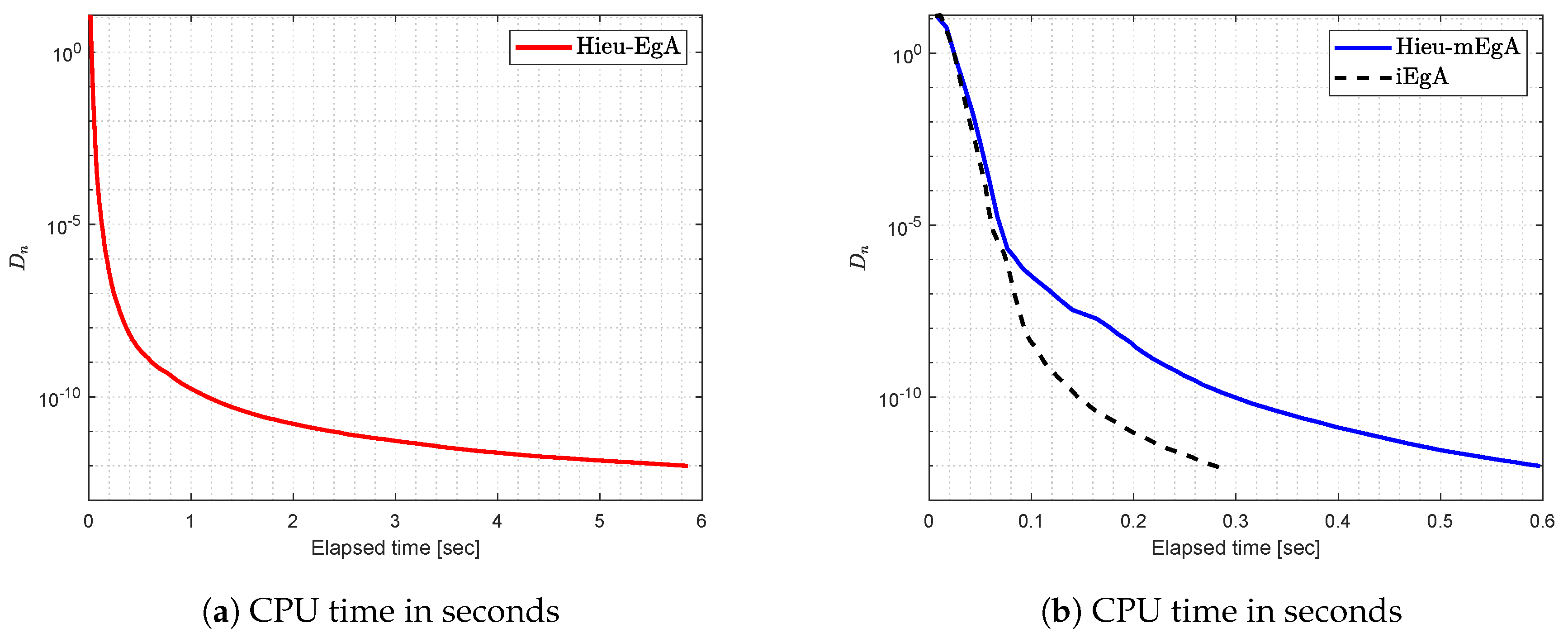
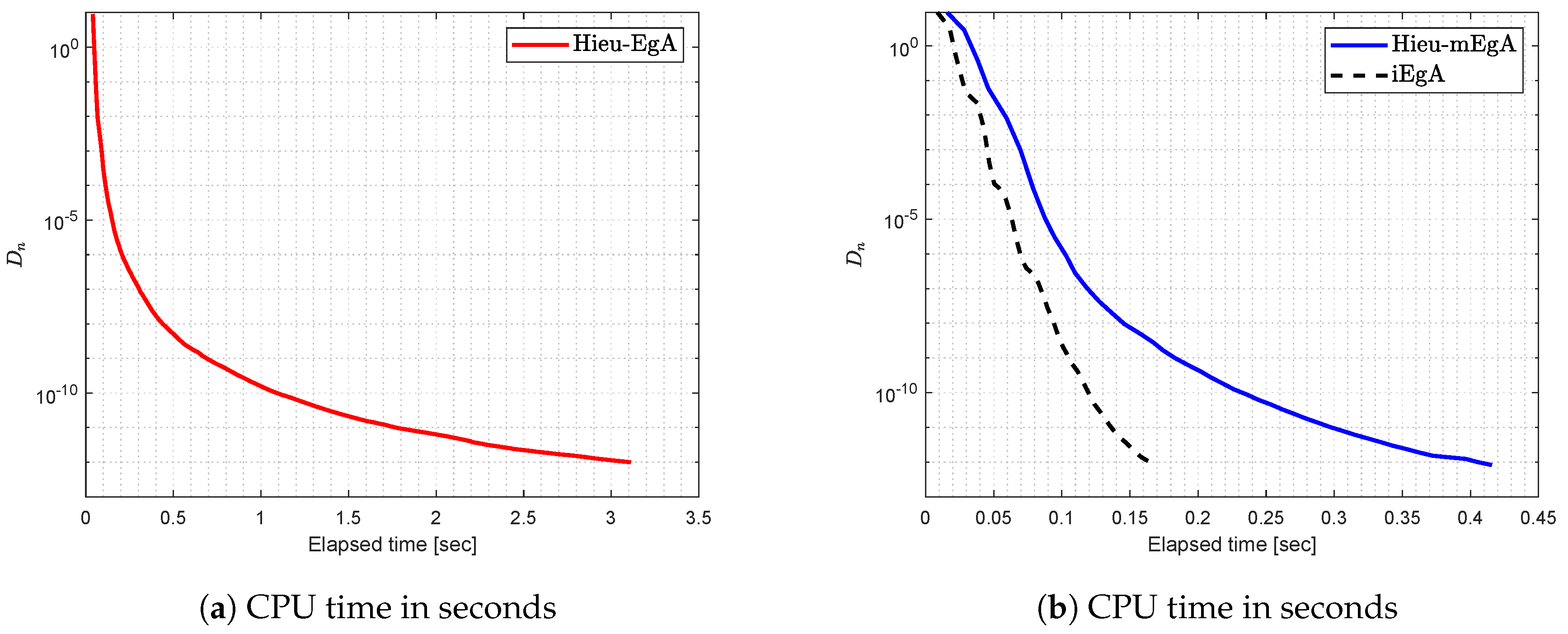
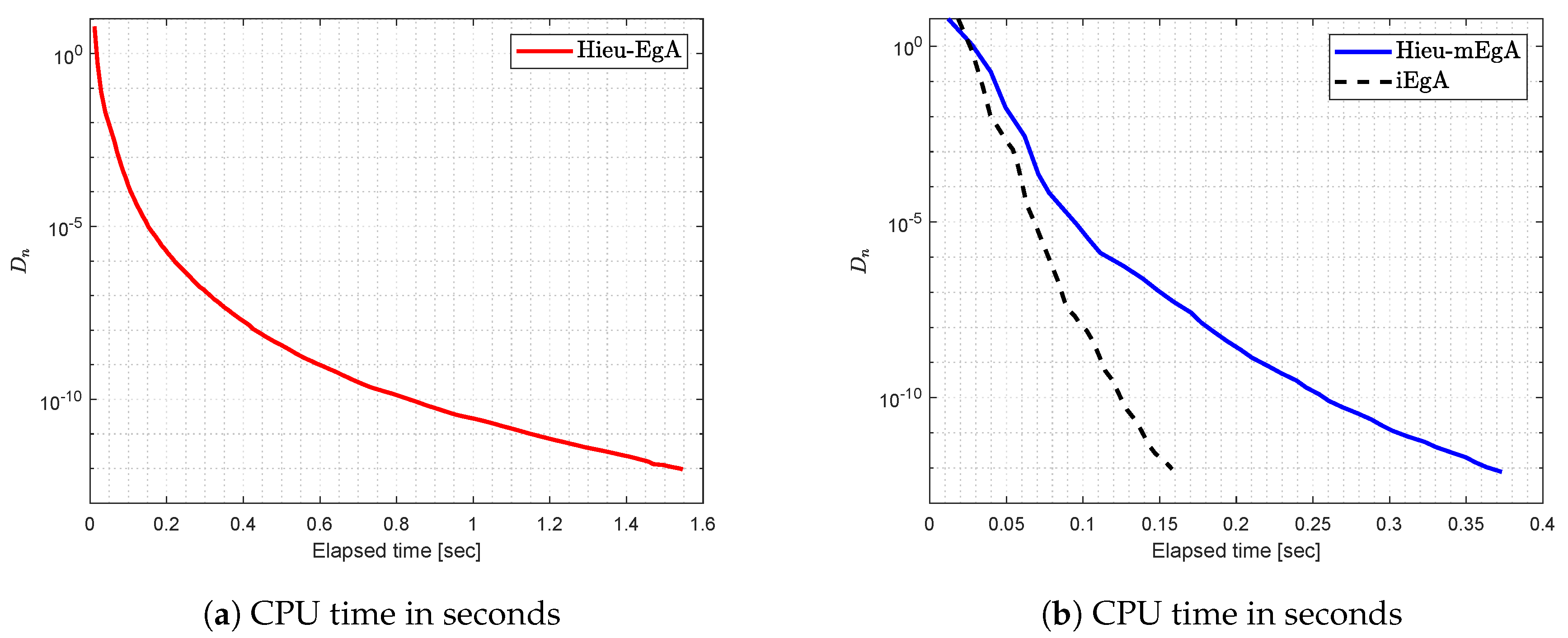
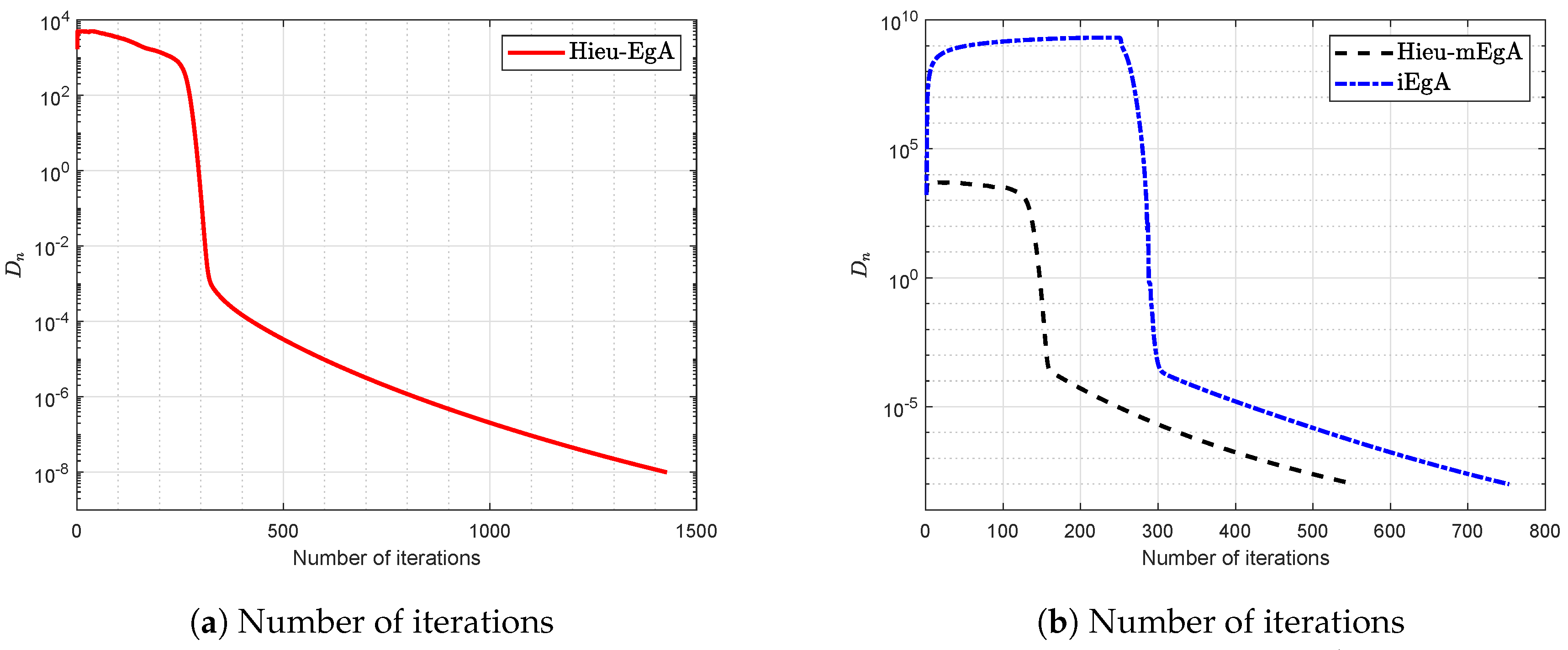
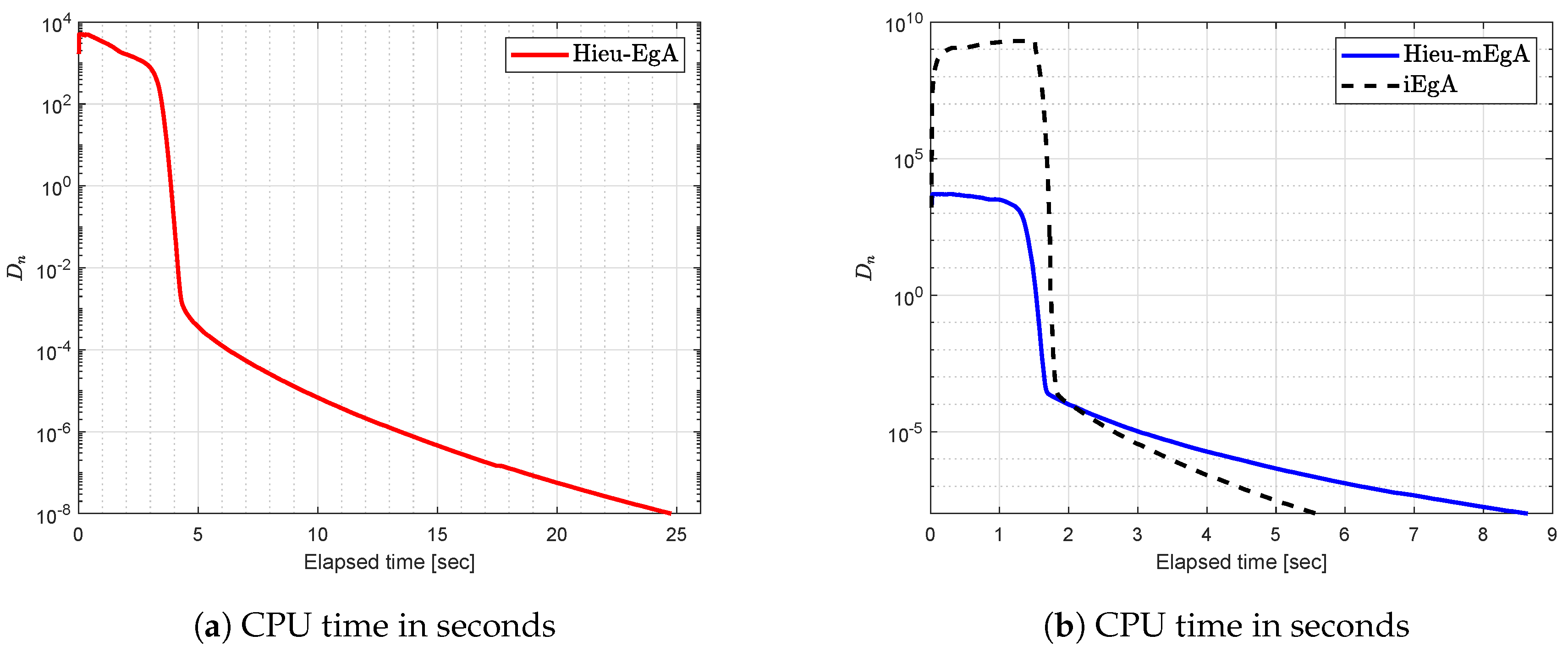
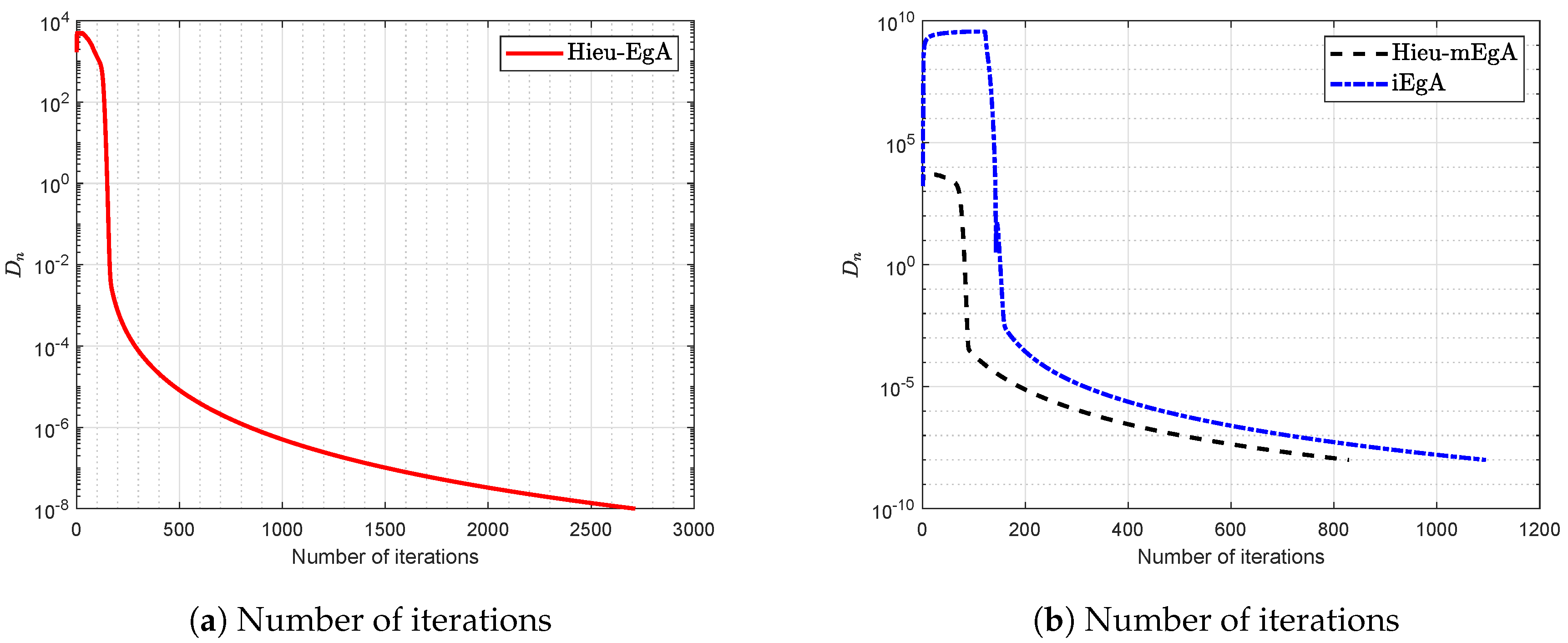
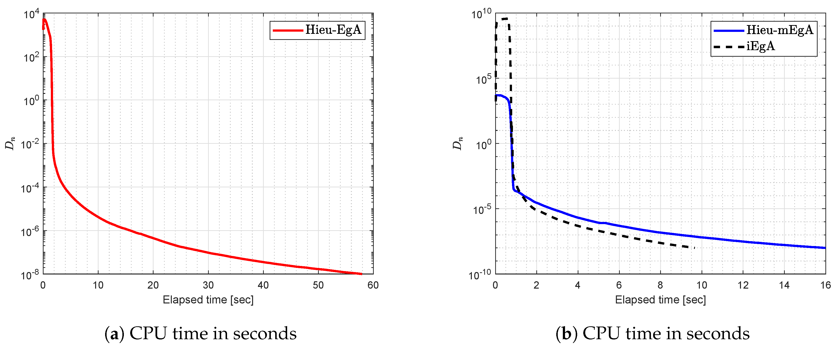
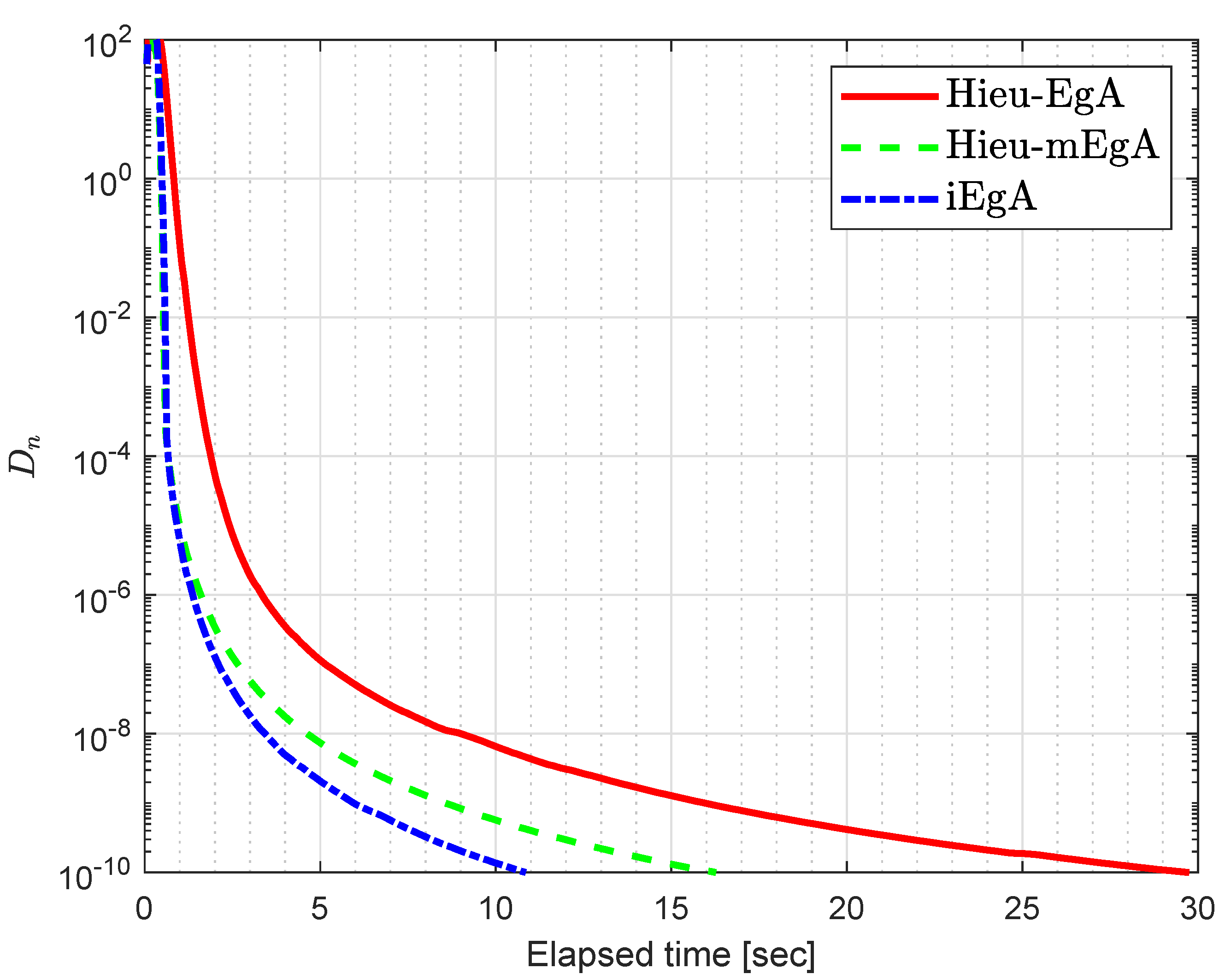
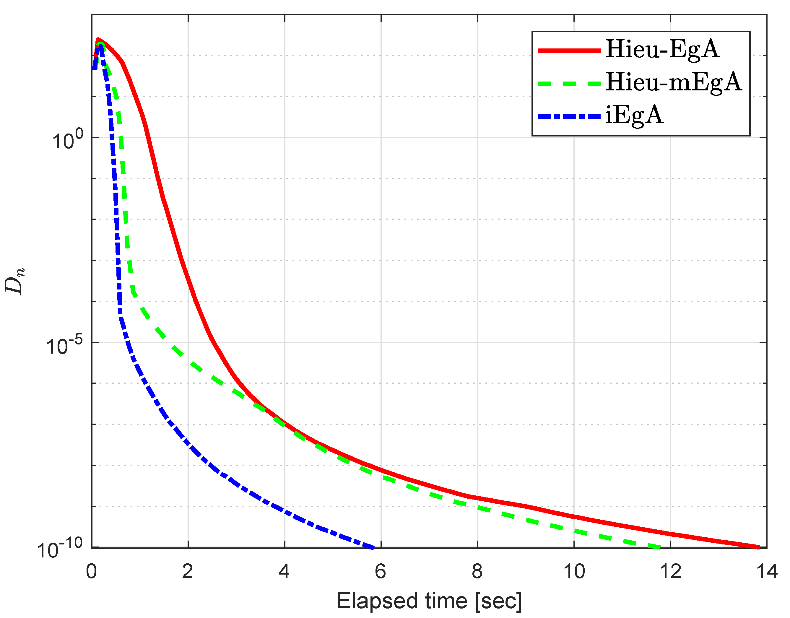
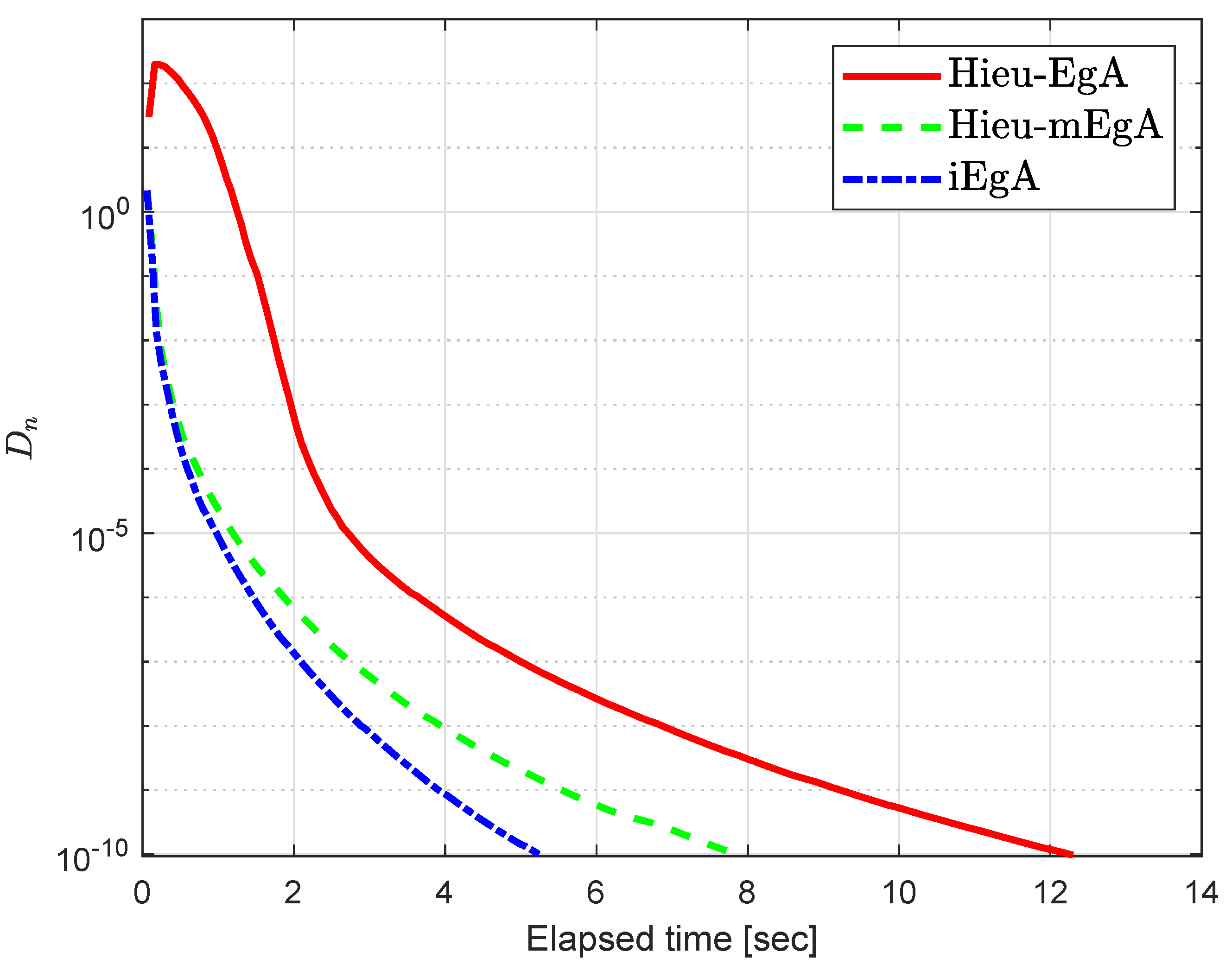
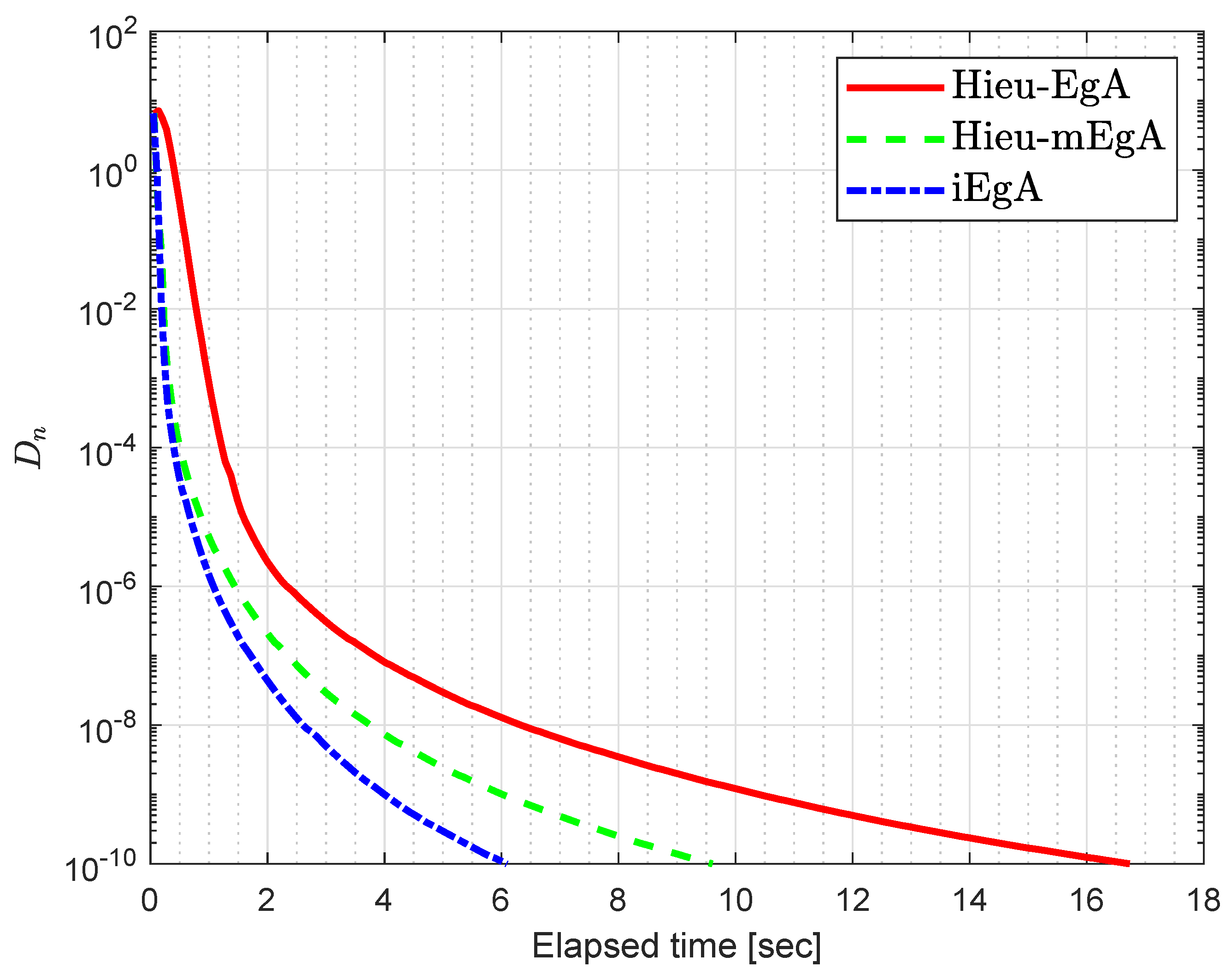
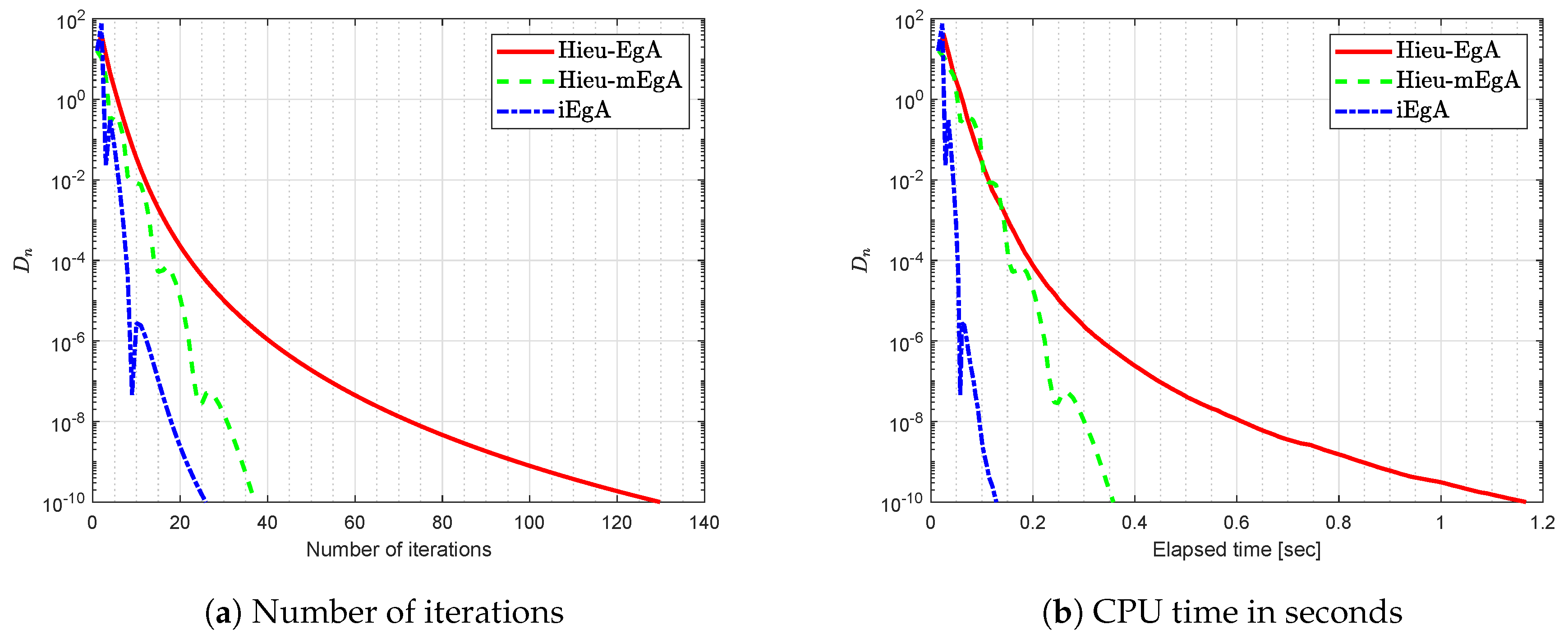
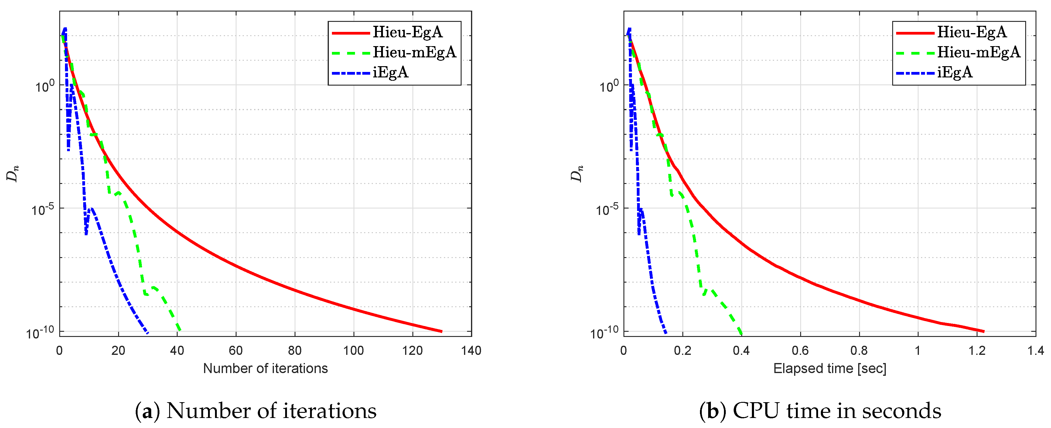
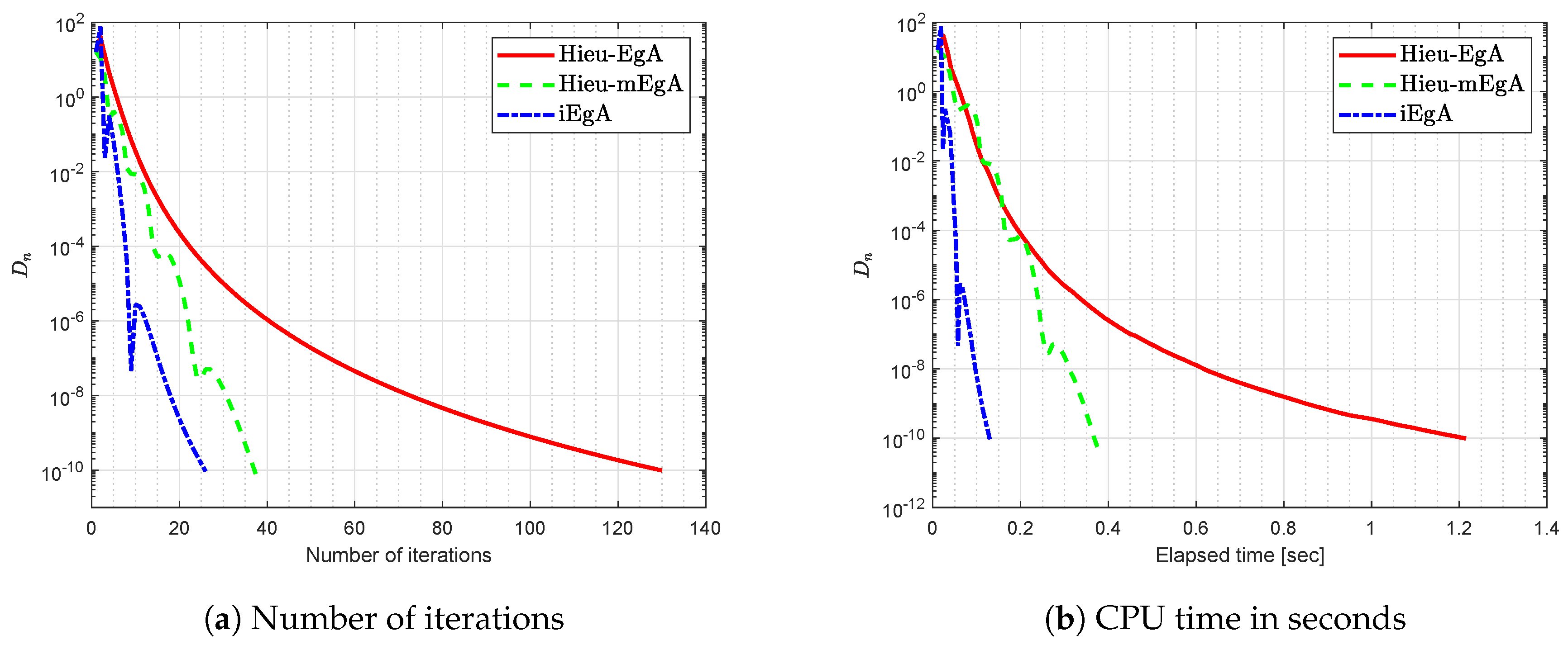
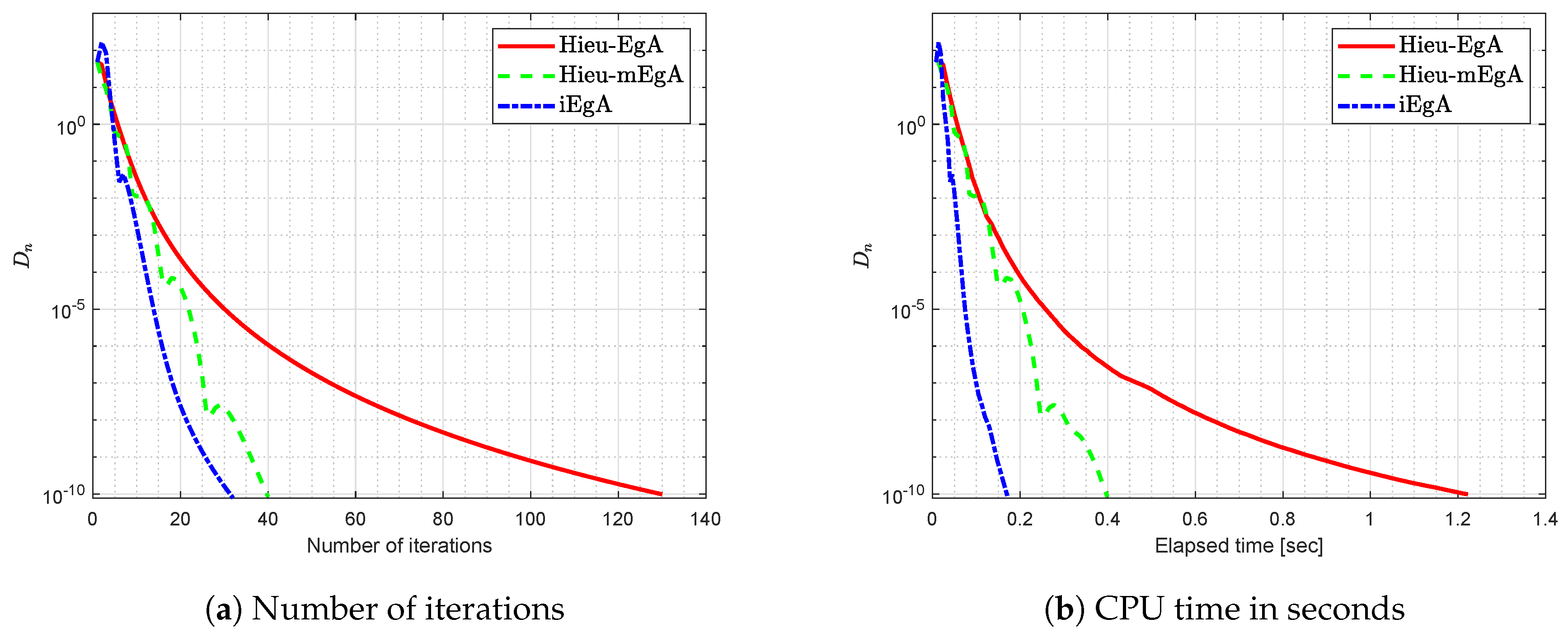
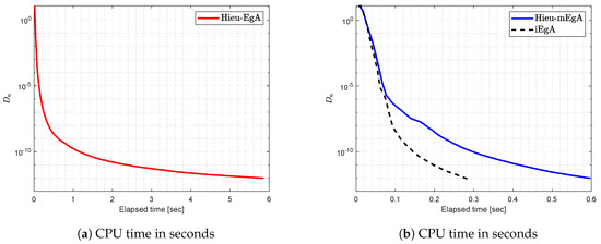
Numerical findings are summarized in this section to demonstrate the effectiveness of the proposed methods. The following control parameters are used in this section.

(1)

For Hieu et al. [26] (Hieu-EgA), we use $D_n={\parallel u_n-v_n\parallel }^2.$

(2)

For Hieu et al. [29] (Hieu-mEgA), we use $\theta =0.5$ and $D_n=max\{\parallel u_{n+1}-v_n{\parallel }^2,\parallel u_{n+1}-w_n{\parallel }^2\}.$

(3)

For Algorithm 1 (iEgA), we use ${\alpha }_n=0.50$, ${\beta }_n=0.80,$ and $D_n={\parallel w_n-v_n\parallel }^2.$

Example 1.

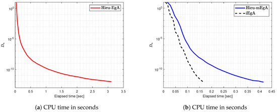
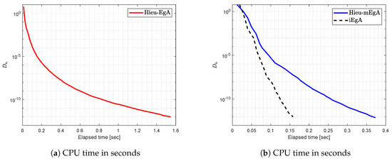
Let bifunction f have the following form

$$f(u,v)=⟨Au+Bv+c,v-u⟩$$

where $c\in {\mathbb{R}}^5$ and A and B are

$$A=\left(\begin{array}{ccccc}3.1& 2& 0& 0& 0\\ 2& 3.6& 0& 0& 0\\ 0& 0& 3.5& 2& 0\\ 0& 0& 2& 3.3& 0\\ 0& 0& 0& 0& 3\end{array}\right)B=\left(\begin{array}{ccccc}1.6& 1& 0& 0& 0\\ 1& 1.6& 0& 0& 0\\ 0& 0& 1.5& 1& 0\\ 0& 0& 1& 1.5& 0\\ 0& 0& 0& 0& 2\end{array}\right)$$

and

$$c=\left(\begin{array}{c}1\\ -2\\ -1\\ 2\\ -1\end{array}\right)$$

where Lipschitz parameters $L_1=L_2=\frac{1}{2}\parallel A-B\parallel$ [26]. The feasible set $\mathcal{K}\subset {\mathbb{R}}^5$ is

$$\mathcal{K}:=\{u\in {\mathbb{R}}^5:-5\le u_i\le 5\}.$$

Table 1 and Figure 1, Figure 2 and Figure 3 show the numerical results by $u_{-1}=u_0=v_0=(1,\cdots ,1)$, and $TOL={10}^{-12}.$

Table 1. Example 1: Numerical values for Figure 1, Figure 2 and Figure 3.

			Hieu-EgA [26]		Hieu-mEgA [29]		iEgA Algorithm 1
n	TOL	${\mathbf{\zeta }}_n$	Iter.	Time	Iter.	Time	Iter.	Time
5	${10}^{-12}$	$\frac{1}{log(n+3)(n+1)}$	320	5.8584	59	0.5979	64	0.2830
5	${10}^{-12}$	$\frac{1}{n+1}$	222	3.1116	43	0.4158	39	0.1696
5	${10}^{-12}$	$\frac{log(n+3)}{n+1}$	122	1.5466	40	0.3732	33	0.1581

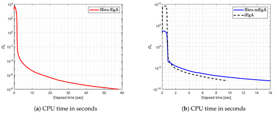
Figure 1. Example 1: Numerical comparison for Algorithm 1 while ${\zeta }_n=\frac{1}{(n+1)log(n+3)}.$

Figure 2. Example 1: Numerical comparison for Algorithm 1 while ${\zeta }_n=\frac{1}{n+1}.$

Figure 3. Example 1: Numerical comparison for Algorithm 1 while ${\zeta }_n=\frac{log(n+3)}{n+1}.$

Example 2.

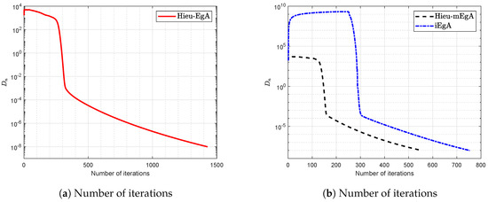
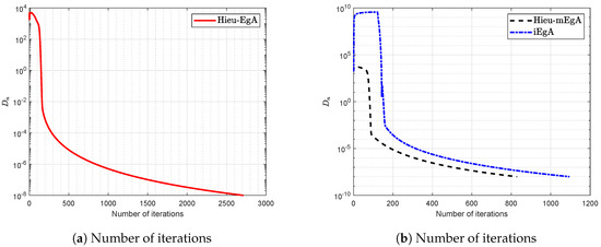
Let a bifunction f be defined on the convex set $\mathcal{K}$ as

$$f(u,v)=⟨(B{B}^T+S+D)u,v-u⟩,$$

where B is a $50\times 50$ matrix, S is a $50\times 50$ skew-symmetric matrix, and D is a $50\times 50$ diagonal matrix. The set $\mathcal{K}\subset {\mathbb{R}}^{50}$ is defined by

$$\mathcal{K}:=\{u\in {\mathbb{R}}^{50}:Au\le b\}$$

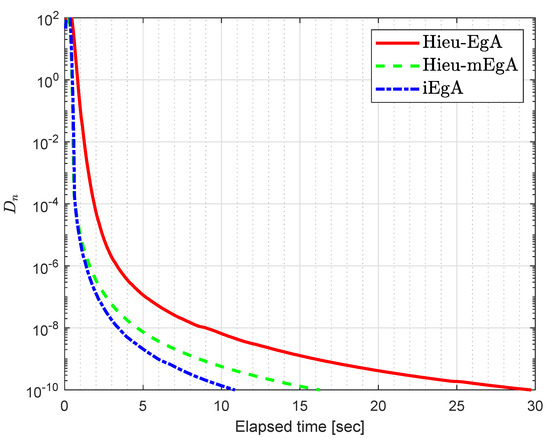
with matrix A as $100\times 50$ and vector b as a non-negative vector. Observe that f is monotone and Lipschitz-type constants are $c_1=c_2=\frac{\parallel B{B}^T+S+D\parallel }{2}.$ We generate random matrices in our case [$B=rand\left(n\right),$$C=rand\left(n\right),$$S=0.5C-0.5C^T,$$D=diag\left(rand\right(n,1\left)\right)$] and the numerical findings regarding Example 2 are shown in Figure 4, Figure 5, Figure 6 and Figure 7 with $u_{-1}=u_0=v_0=(1,\cdots ,1)$ and $TOL={10}^{-12}.$

Figure 4. Example 2: Numerical comparison for Algorithm 1 while ${\zeta }_n=\frac{1}{n+1}.$

Figure 5. Example 2: Numerical comparison for Algorithm 1 while ${\zeta }_n=\frac{1}{n+1}.$

Figure 6. Example 2: Numerical comparison for Algorithm 1 while ${\zeta }_n=\frac{log(n+3)}{n+1}.$

Figure 7. Example 2: Numerical comparison for Algorithm 1 while ${\zeta }_n=\frac{log(n+3)}{n+1}.$

Example 3.

Let $G:{\mathbb{R}}^5\to {\mathbb{R}}^5$ be defined by

$$G\left(u\right)=Au+B\left(u\right)+c,$$

where $n\times n$ symmetric semi-definite matrix A and $B\left(u\right)$ is the function depends on the proximal operator [43] through $h\left(u\right)=\frac{1}{4}{\parallel u\parallel }^4$ such that

$$B\left(u\right)=\underset{v\in {\mathbb{R}}^n}{argmin}\left\{\frac{{\parallel u\parallel }^4}{4}+\frac{1}{2}{\parallel v-u\parallel }^2\right\}.$$

The feasible set $\mathcal{K}$ is considered as

$$\mathcal{K}:=\{u\in {\mathbb{R}}^5:-2\le u_i\le 5\}.$$

The entries of A and c are taken as follows:

$$A=\left(\begin{array}{ccccc}3& 1& 0& 1& 2\\ 1& 5& -1& 0& 1\\ 0& 1& -4& 2& -2\\ 1& 0& 2& 6& -1\\ 2& 1& -2& -1& 4\end{array}\right)c=\left(\begin{array}{c}1\\ -2\\ -1\\ 2\\ -1\end{array}\right)$$

Figure 8, Figure 9, Figure 10 and Figure 11 and Table 2 show the numerical results by using $u_{-1}=u_0=v_0=(1,\cdots ,1)$ and $TOL={10}^{-12}.$

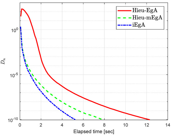
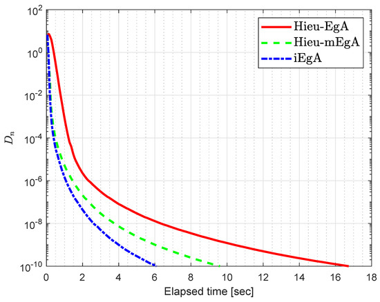
Figure 8. Example 3: Numerical comparison for Algorithm 1 while ${\zeta }_n=\frac{1}{(n+1)log(n+3)}.$

Figure 9. Example 3: Numerical comparison for Algorithm 1 while ${\zeta }_n=\frac{1}{n+1}.$

Figure 10. Example 3: Numerical comparison for Algorithm 1 while ${\zeta }_n=\frac{log(n+3)}{n+1}.$

Figure 11. Example 3: Numerical comparison for Algorithm 1 while ${\zeta }_n=\frac{1}{\sqrt{n+1}}.$

Table 2. Example 3: Numerical results for Figure 8, Figure 9, Figure 10 and Figure 11.

			Hieu-EgA [26]		Hieu-mEgA [29]		iEgA Algorithm 1
n	TOL	${\mathbf{\zeta }}_n$	Iter.	Time	Iter.	Time	Iter.	Time
5	${10}^{-10}$	$\frac{1}{(n+1)log(n+3)}$	440	29.7625	190	16.2712	247	10.8531
5	${10}^{-10}$	$\frac{1}{n+1}$	198	13.8482	104	11.8096	145	5.8483
5	${10}^{-10}$	$\frac{log(n+3)}{n+1}$	178	12.2979	98	7.8478	120	5.2870
5	${10}^{-10}$	$\frac{1}{\sqrt{n+1}}$	251	16.7337	110	9.6097	148	6.0004

Example 4.

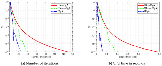
Suppose that $\mathcal{K}\subset G:{\mathbb{R}}^2\to {\mathbb{R}}^2$ is defined by

$$G\left(\begin{array}{c}{v}_1\\ v_2\end{array}\right)=\left(\begin{array}{c}{v}_1+v_2+sin\left(v_1\right)\\ -v_1+v_2+sin\left(v_2\right)\end{array}\right),forall(v_1,v_2)\in {\mathbb{R}}^2.$$

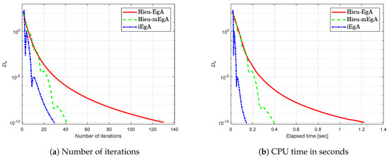
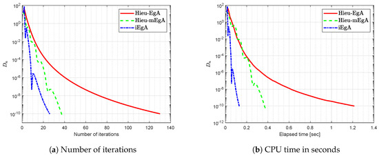
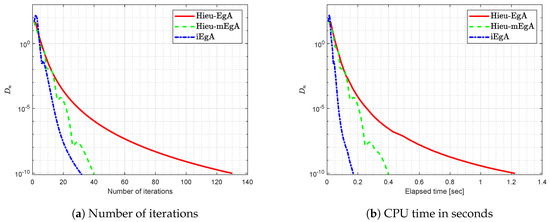
where $\mathcal{K}=[-5,5]\times [-5,5].$ It is easy that G is Lipschitz continuous and strongly pseudomonotone operator. Figure 12, Figure 13, Figure 14 and Figure 15 show the numerical results with $u_{-1}=u_0=v_0$ and $TOL={10}^{-10}.$

Figure 12. Example 4: Numerical comparison for Algorithm 1 while $u_0=(1,1)$ and ${\zeta }_n=\frac{1}{n+1}.$

Figure 13. Example 4: Numerical comparison for Algorithm 1 while $u_0=(4,4)$ and ${\zeta }_n=\frac{1}{n+1}.$

Figure 14. Example 4: Numerical comparison for Algorithm 1 while $u_0=(-1,-1)$ and ${\zeta }_n=\frac{1}{n+1}.$

Figure 15. Example 4: Numerical comparison for Algorithm 1 while $u_0=(-2,-2)$ and ${\zeta }_n=\frac{1}{n+1}.$

5. Conclusions

In this paper, we set up a new method by combining an inertial term with an extragradient method for solving a family of strongly pseudomonotone equilibrium problems. The introduced method involves a sequence of diminishing and non-summable step size rule and the method operates without previous information of the Lipschitz-type constants. Four numerical examples are described to show the computational performance of the proposed method in relation to other existing methods. Numerical experiments clearly point out that the method with an inertial term performs better than those without an inertial term.

References

- Blum, E. From optimization and variational inequalities to equilibrium problems. Math. Stud. 1994, 63, 123–145. [Google Scholar]
- Fan, K. A Minimax Inequality and Applications, Inequalities III; Shisha, O., Ed.; Academic Press: New York, NY, USA, 1972. [Google Scholar]
- Bianchi, M.; Schaible, S. Generalized monotone bifunctions and equilibrium problems. J. Optim. Theory Appl. 1996, 90, 31–43. [Google Scholar] [CrossRef]
- Bigi, G.; Castellani, M.; Pappalardo, M.; Passacantando, M. Existence and solution methods for equilibria. Eur. J. Oper. Res. 2013, 227, 1–11. [Google Scholar] [CrossRef]
- Muu, L.; Oettli, W. Convergence of an adaptive penalty scheme for finding constrained equilibria. Nonlinear Anal. Theory Methods Appl. 1992, 18, 1159–1166. [Google Scholar] [CrossRef]
- Combettes, P.L.; Hirstoaga, S.A. Equilibrium programming in Hilbert spaces. J. Nonlinear Convex Anal. 2005, 6, 117–136. [Google Scholar]
- Antipin, A. Equilibrium programming: Proximal methods. Comput. Math. Math. Phys. 1997, 37, 1285–1296. [Google Scholar]
- Giannessi, F.; Maugeri, A.; Pardalos, P.M. Equilibrium Problems: Nonsmooth Optimization and Variational Inequality Models; Springer Science & Business Media: Berlin/Heidelberg, Germany, 2006; Volume 58. [Google Scholar]
- Dafermos, S. Traffic Equilibrium and Variational Inequalities. Transp. Sci. 1980, 14, 42–54. [Google Scholar] [CrossRef]
- Todorčević, V. Harmonic Quasiconformal Mappings and Hyperbolic Type Metrics; Springer International Publishing: Berlin/Heidelberg, Germany, 2019. [Google Scholar] [CrossRef]
- ur Rehman, H.; Kumam, P.; Cho, Y.J.; Yordsorn, P. Weak convergence of explicit extragradient algorithms for solving equilibirum problems. J. Inequalities Appl. 2019, 2019. [Google Scholar] [CrossRef]
- ur Rehman, H.; Kumam, P.; Je Cho, Y.; Suleiman, Y.I.; Kumam, W. Modified Popov’s explicit iterative algorithms for solving pseudomonotone equilibrium problems. Optim. Methods Softw. 2020, 1–32. [Google Scholar] [CrossRef]
- Todorčević, V. Subharmonic behavior and quasiconformal mappings. Anal. Math. Phys. 2019, 9, 1211–1225. [Google Scholar] [CrossRef]
- Koskela, P.; Manojlović, V. Quasi-Nearly Subharmonic Functions and Quasiconformal Mappings. Potential Anal. 2011, 37, 187–196. [Google Scholar] [CrossRef]
- ur Rehman, H.; Kumam, P.; Abubakar, A.B.; Cho, Y.J. The extragradient algorithm with inertial effects extended to equilibrium problems. Comput. Appl. Math. 2020, 39. [Google Scholar] [CrossRef]
- Hammad, H.A.; ur Rehman, H.; la Sen, M.D. Advanced Algorithms and Common Solutions to Variational Inequalities. Symmetry 2020, 12, 1198. [Google Scholar] [CrossRef]
- Hieu, D.V.; Quy, P.K.; Vy, L.V. Explicit iterative algorithms for solving equilibrium problems. Calcolo 2019, 56. [Google Scholar] [CrossRef]
- Hieu, D.V. New inertial algorithm for a class of equilibrium problems. Numer. Algorithms 2018, 80, 1413–1436. [Google Scholar] [CrossRef]
- Anh, P.K.; Hai, T.N. Novel self-adaptive algorithms for non-Lipschitz equilibrium problems with applications. J. Glob. Optim. 2018, 73, 637–657. [Google Scholar] [CrossRef]
- Anh, P.N.; Anh, T.T.H.; Hien, N.D. Modified basic projection methods for a class of equilibrium problems. Numer. Algorithms 2017, 79, 139–152. [Google Scholar] [CrossRef]
- ur Rehman, H.; Kumam, P.; Kumam, W.; Shutaywi, M.; Jirakitpuwapat, W. The Inertial Sub-Gradient Extra-Gradient Method for a Class of Pseudo-Monotone Equilibrium Problems. Symmetry 2020, 12, 463. [Google Scholar] [CrossRef]
- ur Rehman, H.; Kumam, P.; Argyros, I.K.; Deebani, W.; Kumam, W. Inertial Extra-Gradient Method for Solving a Family of Strongly Pseudomonotone Equilibrium Problems in Real Hilbert Spaces with Application in Variational Inequality Problem. Symmetry 2020, 12, 503. [Google Scholar] [CrossRef]
- Flåm, S.D.; Antipin, A.S. Equilibrium programming using proximal-like algorithms. Math. Program. 1996, 78, 29–41. [Google Scholar] [CrossRef]
- Tran, D.Q.; Dung, M.L.; Nguyen, V.H. Extragradient algorithms extended to equilibrium problems. Optimization 2008, 57, 749–776. [Google Scholar] [CrossRef]
- Korpelevich, G. The extragradient method for finding saddle points and other problems. Matecon 1976, 12, 747–756. [Google Scholar]
- Hieu, D.V. New extragradient method for a class of equilibrium problems in Hilbert spaces. Appl. Anal. 2017, 97, 811–824. [Google Scholar] [CrossRef]
- Polyak, B. Some methods of speeding up the convergence of iteration methods. USSR Comput. Math. Math. Phys. 1964, 4, 1–17. [Google Scholar] [CrossRef]
- Beck, A.; Teboulle, M. A Fast Iterative Shrinkage-Thresholding Algorithm for Linear Inverse Problems. SIAM J. Imaging Sci. 2009, 2, 183–202. [Google Scholar] [CrossRef]
- Hieu, D.V.; Cho, Y.J.; bin Xiao, Y. Modified extragradient algorithms for solving equilibrium problems. Optimization 2018, 67, 2003–2029. [Google Scholar] [CrossRef]
- Rehman, H.U.; Kumam, P.; Dong, Q.L.; Peng, Y.; Deebani, W. A new Popov’s subgradient extragradient method for two classes of equilibrium programming in a real Hilbert space. Optimization 2020, 1–36. [Google Scholar] [CrossRef]
- Yordsorn, P.; Kumam, P.; ur Rehman, H.; Ibrahim, A.H. A Weak Convergence Self-Adaptive Method for Solving Pseudomonotone Equilibrium Problems in a Real Hilbert Space. Mathematics 2020, 8, 1165. [Google Scholar] [CrossRef]
- Yordsorn, P.; Kumam, P.; Rehman, H.U. Modified two-step extragradient method for solving the pseudomonotone equilibrium programming in a real Hilbert space. Carpathian J. Math. 2020, 36, 313–330. [Google Scholar]
- Fan, J.; Liu, L.; Qin, X. A subgradient extragradient algorithm with inertial effects for solving strongly pseudomonotone variational inequalities. Optimization 2019, 1–17. [Google Scholar] [CrossRef]
- Thong, D.V.; Hieu, D.V. Inertial extragradient algorithms for strongly pseudomonotone variational inequalities. J. Comput. Appl. Math. 2018, 341, 80–98. [Google Scholar] [CrossRef]
- Censor, Y.; Gibali, A.; Reich, S. The Subgradient Extragradient Method for Solving Variational Inequalities in Hilbert Space. J. Optim. Theory Appl. 2010, 148, 318–335. [Google Scholar] [CrossRef] [PubMed]
- ur Rehman, H.; Kumam, P.; Argyros, I.K.; Alreshidi, N.A.; Kumam, W.; Jirakitpuwapat, W. A Self-Adaptive Extra-Gradient Methods for a Family of Pseudomonotone Equilibrium Programming with Application in Different Classes of Variational Inequality Problems. Symmetry 2020, 12, 523. [Google Scholar] [CrossRef]
- ur Rehman, H.; Kumam, P.; Argyros, I.K.; Shutaywi, M.; Shah, Z. Optimization Based Methods for Solving the Equilibrium Problems with Applications in Variational Inequality Problems and Solution of Nash Equilibrium Models. Mathematics 2020, 8, 822. [Google Scholar] [CrossRef]
- ur Rehman, H.; Kumam, P.; Shutaywi, M.; Alreshidi, N.A.; Kumam, W. Inertial Optimization Based Two-Step Methods for Solving Equilibrium Problems with Applications in Variational Inequality Problems and Growth Control Equilibrium Models. Energies 2020, 13, 3292. [Google Scholar] [CrossRef]
- Attouch, F.A.H. An Inertial Proximal Method for Maximal Monotone Operators via Discretization of a Nonlinear Oscillator with Damping. Set-Valued Var. Anal. 2001, 9, 3–11. [Google Scholar] [CrossRef]
- Heinz, H.; Bauschke, P.L. Convex Analysis and Monotone Operator Theory in Hilbert Spaces, 2nd ed.; CMS Books in Mathematics; Springer International Publishing: Berlin/Heidelberg, Germany, 2017. [Google Scholar]
- Ofoedu, E. Strong convergence theorem for uniformly L-Lipschitzian asymptotically pseudocontractive mapping in real Banach space. J. Math. Anal. Appl. 2006, 321, 722–728. [Google Scholar] [CrossRef]
- Tiel, J.V. Convex Analysis: An Introductory Text, 1st ed.; Wiley: New York, NY, USA, 1984. [Google Scholar]
- Kreyszig, E. Introductory Functional Analysis with Applications, 1st ed.; Wiley: New York, NY, USA, 1978. [Google Scholar]
Publisher’s Note: MDPI stays neutral with regard to jurisdictional claims in published maps and institutional affiliations. |
© 2020 by the authors. Licensee MDPI, Basel, Switzerland. This article is an open access article distributed under the terms and conditions of the Creative Commons Attribution (CC BY) license (http://creativecommons.org/licenses/by/4.0/).