Article

Mathematical and Numerical Modeling of On-Threshold Modes of 2-D Microcavity Lasers with Piercing Holes

by
Alexander O. Spiridonov
1,*,
Evgenii M. Karchevskii
2 and
Alexander I. Nosich
3
1
Laboratory of Computational Technologies and Computer Modeling, Kazan Federal University, 18 Kremlevskaya st., 420008 Kazan, Russia
2
Department of Applied Mathematics, Kazan Federal University, 18 Kremlevskaya st., 420008 Kazan, Russia
3
Laboratory of Micro and Nano Optics, Institute of Radio-Physics and Electronics NASU, vul. Proskury 12, 61085 Kharkiv, Ukraine
*
Author to whom correspondence should be addressed.
Axioms 2019, 8(3), 101; https://doi.org/10.3390/axioms8030101
Submission received: 31 July 2019 / Revised: 18 August 2019 / Accepted: 19 August 2019 / Published: 1 September 2019

Abstract

:
This study considers the mathematical analysis framework aimed at the adequate description of the modes of lasers on the threshold of non-attenuated in time light emission. The lasers are viewed as open dielectric resonators equipped with active regions, filled in with gain material. We introduce a generalized complex-frequency eigenvalue problem for such cavities and prove important properties of the spectrum of its eigensolutions. This involves reduction of the problem to the set of the Muller boundary integral equations and their discretization with the Nystrom technique. Embedded into this general framework is the application-oriented lasing eigenvalue problem, where the real emission frequencies and the threshold gain values together form two-component eigenvalues. As an example of on-threshold mode study, we present numerical results related to the two-dimensional laser shaped as an active equilateral triangle with a round piercing hole. It is demonstrated that the threshold of lasing and the directivity of light emission, for each mode, can be efficiently manipulated with the aid of the size and, especially, the placement of the piercing hole, while the frequency of emission remains largely intact.

1. Introduction

Lasers are complicated photonic sources of light, and their understanding and design have been always closely tied to efficient and reliable modeling. Here, from the onset of research into lasers, it became clear that purely electromagnetic analysis of laser cavities is very useful. Therefore, it was also applied to the microcavity lasers, introduced in the 1990s, where the light is confined inside a transparent dielectric cavity of micrometer size. For arbitrary shapes, the mode analysis was performed usually with the aid of geometrical optics (see review papers [1,2,3,4,5] and references therein) and, for simple circular-disk shapes, with Maxwell equations (see reviews [6,7,8]). On the one hand, such analysis enabled one to explain the fact that the lasers emitted light on discrete frequencies, via the concept of natural modes of laser cavities, i.e., discrete eigenstates of the electromagnetic field as solutions to eigenvalue problems. This made the frequencies of lasing predictable, although the eigenfrequencies of open cavities are only complex-valued while lasers emit light that does not decay in time.
On the other hand, such analysis was still unable to explain another fundamental property of laser, namely, that each mode started lasing only above a certain threshold. This term reflects the fact that laser cavities differ from more conventional microwave cavities by the presence of so-called active regions. The latter is filled in with gain material, i.e., a material, which is able, at the microscopic level, to emit the light due to certain quantum-mechanical mechanisms. To enable such mechanisms to work, one has to provide an external influx of power called pumping, and the term threshold relates to the intensity of the pumping.
Therefore, to explain the threshold of lasing, the active region has to be introduced into the electromagnetic model of the laser. Then, immediately, it can be found that the eigenfrequencies of the open cavities equipped with active regions can obtain purely real values. Moreover, this happens when the gain index of the active region material takes a value, specific for each mode of the cavity. After that, it becomes evident that the classical electromagnetic eigenvalue problem should be modified to address the threshold of gain (proportional to pump power), together with the real-valued frequency, as two components of an eigenvalue. This idea nicely agrees with the experimentally observed fact that each mode of the laser cavity has a different threshold pump power, and its value is closely tied to the mode field structure.
Such observations lied in the core of the lasing eigenvalue problem (LEP) approach, suggested in [9,10,11] and applied to the on-threshold analysis of lasing modes of 2-D circular [10,11,12,13], and non-circular cavities: Limacon [14], ellipse [15], kite [16], square and other regular polygons [17]. As is easy to see, a presence of both active regions with gain material and lossy regions with absorptive material can be taken into account, in LEP, without any difficulty. Therefore, recently on-threshold mode analyses were published for the plasmonic nanolasers based on a silver strip in a quantum wire [18] and a silver tube in such a wire [19], assumed to be made of gain material. In today’s laser engineering, the direction of research associated with periodic arrays of metal or dielectric nanoparticles and nanowires, placed inside or on top of the quantum well (active layer) is very interesting and much promising. These configurations can be also treated with LEP approach. This was demonstrated by the analysis of modes of an infinite grating of circular quantum wires [20] and a binary grating made of pairs of silver and quantum wires [21]. In the latter case, it was found that the localized surface-plasmon modes have higher thresholds than the so-called lattice or grating modes, appearing thanks to periodicity. Still, from our point of view, the most impressive demonstration of the predictive power of LEP in the laser physics is the recent explanation of the mystery: Why elliptic or similar 2-D lasers emit light not on whispering-gallery modes but on bow-tie modes [15]. As we showed in that paper, the mystery is solved if one introduces a centrally located partial active region, mimicking realistic injection electrode, which better overlaps with the bow-tie mode fields than with the whispering-gallery ones.
Note that other LEP-like formulations exist [22,23,24,25,26]. They differ from what is presented by us in the way of introduction of the gain, for instance, as the imaginary part of not the refractive index but of the dielectric permittivity in active region, or a product of the imaginary part of the refractive index and the frequency.
Although the usefulness of LEP is quite obvious, its comprehensive mathematical theory has not been provided so far, however, certain efforts were presented in [27]. Development of such theory is actually the aim of our work. Here, the LEP grounding meets some difficulties. These difficulties are in the fact that the theory of operator-valued functions of a two-component vector parameter is not yet sufficiently developed. Therefore, to achieve our goal, we introduce a generalized complex-frequency eigenvalue problem (GCFEP) for the modes of open cavity with active region.
We prove the theorems on the properties of its spectrum, i.e., the set of complex eigenfrequencies, each of which depends continuously on the additional real parameter, the gain/loss index in the active/absorptive region. Then, we observe that the LEP is embedded in GCFEP as a particular case. Further, we discuss the reduction of GCFEP and LEP for 2-D lasers to the search of the spectrum of the coupled Muller boundary integral equations and discretization of the latter equations using the Nystrom algorithm. The convergence of that algorithm is proved. We illustrate the presented approach by computing the frequencies, the threshold gains, and the modal fields of the 2-D laser shaped as an active equilateral triangle with a round piercing hole. Note that the effect of piercing holes on the directionality of emission of laser was studied in [28], however, only with the aid of geometrical optics, which is sufficiently accurate only for huge-size cavities.

2. Analytical Regularization of the Generalized Complex-Frequency Eigenvalue Problem

In the beginning of this section, we consider the statement of GCFEP for 2-D optical resonators with piercing holes. The problem statement combines two physical models of mode emission from 2-D microcavities: Complex-frequency eigenvalue problem (CFEP) and LEP (see, e.g., [16,
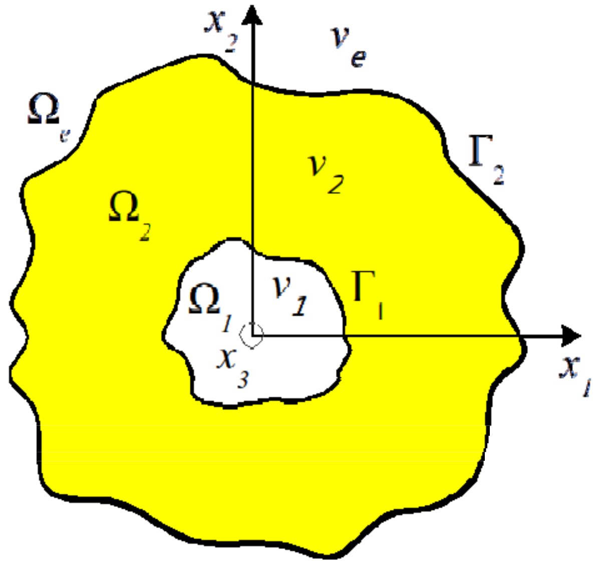
29], respectively). The geometry of investigated microcavity lasers is shown in Figure 1. Here, the domain Ω 1 is a hole in the cavity, the main body of the resonator is Ω 2 , and the unbounded domain Ω e is the environment of the resonator. These regions are separated by the boundaries Γ 1 and Γ 2 . We assume that they are twice continuously differentiable curves, and n is the outer normal unit vector ether to Γ 1 or Γ 2 , depending on the context.
We also assume that the refractive index ν e of the environment of the resonator is positive and coincides with the refractive index ν 1 of the piercing hole. This value is given, we write it as ν 1 = ν e = α e > 0 . The refractive index in the domain Ω 2 is complex-valued, ν 2 = α a i γ . Here, α a > 0 is the given real part of ν 2 , and γ is the real-valued parameter of GCFEP (the loss/gain index). If the cavity is passive and lossless, then γ = 0 . For lossy cavities, γ < 0 . If the region Ω 2 is filled in with a gain material, then γ > 0 .
Besides, we assume that the electromagnetic field does not depend on the variable x 3 and depends on time as ~ e x p ( i k c t ) . Here, as usual, c denotes the speed of light in vacuum. We suppose that the wavenumber k is complex-valued and unknown (it is the eigenvalue of GCFEP). Following [30], we are looking for k on the Riemann surface L of the function ln k . Since the electromagnetic field does not vary along the x 3 axis, all E- and H-components are represented in terms of a scalar eigenfunction of GCFEP, u U \ 0 , which is either the E 3 or H 3 component for E- and H-polarization, respectively. By the symbol U we denote the space of all complex-valued continuous on Ω ¯ 1 and Ω ¯ 2 and twice continuously differentiable on Ω 1 and Ω 2 functions.
For a given γ , an eigenfunction of GCFEP u U \ 0 together with a corresponding eigenvalue k L have to satisfy the Helmholtz equations,
Δ u + k e 2 u = 0 , x Ω 1 , e ,
Δ u + k a 2 u = 0 , x Ω 2 ,
the transmission conditions,
u = u + , η e u n = η a u + n , x Γ 1 ,
u = u + , η a u n = η e u + n , x Γ 2 ,
and the outgoing Reichardt radiation condition [30,31],
u ( r , φ ) = l = a l H l ( 1 ) k e r e i l φ , r R 0 .
Here, k a , e = k ν a , e is the wavenumber in the corresponding region. The coefficients in (3) and (4) depend on polarization, namely, η a , e = ν a , e 2 and b η a , e = 1 for the H-polarized and E-polarized fields, respectively. As usual, we denote the Hankel function of the first kind and index l by H l ( 1 ) ( z ) , and the polar coordinates of the point x by r and φ . The limit values of the function u U in boundary conditions (3) and (4) have the following definitions (see, e.g., [32], p. 68): The limits
u ± n ( x ) = lim h + 0 ( n ( x ) , grad u ( x ± h n ( x ) ) , x Γ 1 , 2 ,
are supposed to exist uniformly on Γ 1 , 2 . It is important to note that for any eigenfunction of GCFEP, the series in (5) converges uniformly and absolutely and is infinitely termwise differentiable [30].
Denote the principal sheet of L by L 0 and assume that it has a branch cut along the negative imaginary semi-axis. There are three types of eigenfunctions of GCFEP depending on the location of the corresponding eigenvalue k L 0 . If Im k = 0 , then (5) is equivalent to the usual Sommerfeld radiation condition,
r i k e u = o 1 r , r .
If Im k > 0 , then u decays exponentially as r , while, if Im k < 0 , then the eigenfunction u exponentially grows at infinity. For our consideration it is important that for any k L , γ , and u satisfying (5), the following equality is true [30,31]:
Γ R u ( y ) G e ( x , y ) n ( y ) d l ( y ) Γ R G e ( x , y ) u ( y ) n ( y ) d l ( y ) = 0 , x Ω e .
Here, G e = i 4 H 0 ( 1 ) ( k e | x y | ) and Γ R is a circle of sufficiently large radius R with the center at x. This fact permits us to investigate all the types of eigenfunctions in one framework.
The imaginary parts of the eigenvalues k L 0 depend on the parameter γ . If γ 0 , then the cavity is passive (lossless or lossy, as it was mentioned above), and the statement of GCFEP coincides exactly with the statement of conventional CFEP [29]. In this case, as follows from the complex Poynting theorem, Im k < 0 for all the eigenvalues k L 0 —see Equation (10) of [11]. If γ > 0 , then the cavity is active, and some of the eigenvalues k can have Im k < K , where K > 0 , i.e., the imaginary part of some k L 0 can be equal to or greater than zero. If there exits γ > 0 , such that the eigenvalue k of GCFEP is positive, then the pair k , γ and the corresponding eigenfunction u satisfy all the conditions of LEP [11,16,27]. Such values of γ are different for different eigenvalues k . They are the values of the threshold material gain that is needed to compensate for the radiation losses and provide not attenuating in the time field function for the corresponding k .
Theorem 1. 
For each γ the positive imaginary semi-axis Im + of L 0 is free of the eigenvalues k of GCFEP.
Proof of Theorem 1. 
We prove this theorem by direct calculations in the same way as the uniqueness theorem for the transmission problem for the Helmholtz equations is proved (see [32], p. 100). Namely, we assume that a triple γ , k Im + , u U satisfy (1)–(5) and apply Green’s theorem (see, e.g., [32], p. 68) to the function u and its complex conjugate in all the domains of the problem. Further, we use the transmission conditions (3), (4) and the condition at infinity (5). Here we note that for any k Im + the function u and all its derivatives exponentially decay at infinity, therefore, all the integrals on the domain Ω e exist. Finally, equating to zero the imaginary parts of both sides of the constructed equality and analyzing they signs, we conclude that the function u is zero on the plane. Thus, u is not an eigenfunction of GCFEP. □
To apply the method of analytical regularization [33,34] for GCFEP, we use the following integral representations of the eigenfunctions u :
u ( x ) = Γ 1 u ( y ) G e ( x , y ) n ( y ) d l ( y ) + Γ 1 G e ( x , y ) u ( y ) n ( y ) d l ( y ) , x Ω 1 ,
u ( x ) = Γ 1 u + ( y ) G e ( x , y ) n ( y ) d l ( y ) Γ 1 G e ( x , y ) u + ( y ) n ( y ) d l ( y ) Γ 2 u ( y ) G a ( x , y ) n ( y ) d l ( y ) + Γ 2 G a ( x , y ) u ( y ) n ( y ) d l ( y ) , x Ω 2 ,
u ( x ) = Γ 2 u + ( y ) G e ( x , y ) n ( y ) d l ( y ) Γ 2 G e ( x , y ) u + ( y ) n ( y ) d l ( y ) , x Ω e .
where G a = i 4 H 0 ( 1 ) ( k a | x y | ) . Equations (9) and (10) are well known (see, e.g., [32], p. 68). Equation (11) is also true since we have (8) for any k L and γ .
Let
u j ( x ) = u + ( x ) = u ( x ) , x Γ j , j = 1 , 2 .
v 1 = η a + η e 2 η e u + n = η a + η e 2 η a u n , x Γ 1 , v 2 = η e + η a 2 η a u + n = η e + η a 2 η e u n ,   x Γ 2 ,
and let C j = C ( Γ j ) be the Banach space of continuous functions on Γ j , j = 1 , 2 , supplied with the maximum norm, C = C 1 × C 2 , and W = C × C . Denote by I the identical operator in the space W. Then GCFEP (1)–(5) is equivalent to the following nonlinear eigenvalue problem [27] (see also [35]):
A ( k , γ ) w = ( I + B ( k , γ ) ) w = 0 .
Here,
B = B 1 1 , 1 B 1 1 , 2 B 1 1 , 3 B 1 1 , 4 B 1 2 , 1 B 1 2 , 2 B 1 2 , 3 B 1 2 , 4 B 2 3 , 1 B 2 3 , 2 B 2 3 , 3 B 2 3 , 4 B 2 4 , 1 B 2 4 , 2 B 2 4 , 3 B 2 4 , 4 , w = u 1 v 1 u 2 v 2 , B j q , s g ( x ) = Γ j K j q , s ( x , y ) g ( y ) d l ( y ) .
The function g denotes either u j or v j , j = 1 , 2 . The kernels have the form [27],
K 1 1 , 1 = K 2 3 , 3 = ( G e ( x , y ) G a ( x , y ) ) n ( y ) , K 1 1 , 2 = K 2 3 , 4 = 2 ( η e G a ( x , y ) η a G e ( x , y ) ) η a + η e ,
K 1 1 , 3 = K 2 3 , 1 = G a ( x , y ) n ( y ) , K 1 1 , 4 = 2 η e G a ( x , y ) η e + η a , K 1 2 , 1 = K 2 4 , 3 = 2 ( G e ( x , y ) G a ( x , y ) ) n ( x ) n ( y ) ,
K 1 2 , 2 = K 2 4 , 4 = 2 η e η a + η e G a ( x , y ) n ( x ) 2 η a η a + η e G e ( x , y ) n ( x ) , K 1 2 , 3 = K 2 4 , 1 = 2 G a ( x , y ) n ( x ) n ( y ) ,
K 1 2 , 4 = K 2 4 , 2 = 2 η e η e + η a G a ( x , y ) n ( x ) , K 2 3 , 2 = 2 η e G a ( x , y ) η a + η e ,
As proved in [27], some of the kernels K j q , s have the logarithmic singularities and all the others are continuous. Therefore, for each k L and γ the operator B ( k , γ ) is compact [27].
Theorem 2. 
The operator A ( k , γ ) has a bounded inverse operator for each γ and k I m + . For any given γ the set of all the eigenvalues k of the operator-valued function A ( k ) can be only a set of discrete points on L having finite algebraic multiplicities. Each eigenvalue k depends continuously on the parameter γ and can appear and disappear only at zero and at infinity on L .
Proof of Theorem 2. 
The first assertion of the theorem is derived directly from the Fredholm alternative (see, e.g. [36], p. 47), the compactness of the operator B ( k , γ ) , and Theorem 1. Arguing as in the proof of Lemmas 1–4 in [27] and following [37], we see that for any given γ the operator-valued function A ( k ) is holomorphic in k L . Therefore, the second assertion of the theorem follows from Proposition A. 8.4, p. 422, [38]. Following Proposition 6.1, p. 1148, [39], we prove that the operator-valued function A ( k , γ ) is jointly continuous at any point ( k , γ ) in L × . Thus, the last assertion of the theorem follows immediately from Theorem 4.3, [40]. □
If γ is less than or equal to zero, then the assertions of Theorem 2 correspond to CFEP, while the following corollary from Theorem 2 describes the set of all the eigenvalues of LEP.
Corollary 1. 
Assume that for some positive γ the intersection of the set of all the eigenvalues k of the operator-valued function A ( k ) and the positive real semi-axis of the principal shit of L is not empty. Then this intersection can be only a set of discrete eigenvalues of A ( k ) having finite algebraic multiplicities.

3. Nyström Method

Now, following [41], p. 69, we present the Nyström method for numerical solution of nonlinear eigenvalue problem (14). Note that this method was applied, in the simplest form, in [16] and then sophisticated in [17], to take full account of possible symmetry lines of a 2-D cavity. Assume that each contour Γ j has a parameterization r j ( t ) = ( r j 1 ( t ) , r j 2 ( t ) ) , where r j 1 ( t ) = f j ( t ) cos t , r j 2 ( t ) = f j ( t ) sin t , and t [ 0 , 2 π ] . We write
L ( t , τ ) = Q ( t , τ ) ln 4 sin 2 t τ 2 + P ( t , τ ) ,
where L = K j q , s , P = P j q , s , Q = Q j q , s , j = 1, 2, q , s = 1 , 2 , 3 , 4 . It is easy to see that all of the following functions are continuous:
Q 1 1 , 1 = Q 2 3 , 3 = ( x y ) n ( y ) | x y | × k e J 1 ( k e | x y | ) k a J 1 ( k a | x y | ) 4 π ,
Q 1 1 , 2 = Q 2 3 , 4 = η e J 0 ( k a | x y | ) η a J 0 ( k e | x y | ) 2 π ( η a + η e ) , Q 1 1 , 3 = Q 2 3 , 1 = k a J 1 ( k a | x y | ) ( x y ) n ( y ) 4 π | x y | ,
Q 1 1 , 4 = η e J 0 ( k a | x y | ) 2 π ( η e + η a ) , Q 2 3 , 2 = 2 η e J 0 ( k a | x y | ) 4 π ( η a + η e ) ,
Q 1 2 , 1 = Q 2 4 , 3 = ( ( x y ) n ( y ) ) ( ( x y ) n ( x ) ) | x y | 2 × k e 2 J 2 ( k e | x y | ) k a 2 J 2 ( k a | x y | ) 4 π k e J 1 ( k e | x y | ) k a J 1 ( k a | x y | ) 4 π × ( n ( x ) n ( y ) ) | x y | ,
Q 1 2 , 2 = Q 1 4 , 4 = ( x y ) n ( x ) | x y | × η e k a J 1 ( k a | x y | ) η a k e J 1 ( k e | x y | ) 2 π ( η a + η e ) ,
Q 1 2 , 3 = Q 2 4 , 1 = k a J 1 ( k a | x y | ) ( n ( x ) n ( y ) ) 4 π | x y | k a 2 J 2 ( k a | x y | ) ( ( x y ) n ( y ) ) ( ( x y ) n ( x ) ) 4 π | x y | 2 ,
Q 1 2 , 4 = Q 2 4 , 2 = η e k a J 1 ( k a | x y | ) ( x y ) n ( x ) 2 π ( η a + η e ) | x y | ,
P j q , s ( t , τ ) = K j q , s ( t , τ ) Q j ( q , s ) ( t , τ ) ln 4 sin 2 t τ 2 .
Let Ξ h = { t l , h } l = 0 2 n 1 be a uniform grid on [ 0 , 2 π ] with the mesh size h = π / n , i.e., t l = t l , h = l h . We approximate the integrals with continuous kernels using the quadrature formula of trapezoidal rule,
0 2 π g ( τ ) d τ h l = 0 2 n 1 g ( t l ) .
For the logarithmic parts of kernels, we use the quadrature formula for approximation of integrands by trigonometric polynomials,
0 2 π l n 4 sin 2 t τ 2 g ( τ ) d τ l = 0 2 n 1 R l ( h ) ( t ) g ( t l ) ,
where
R l ( h ) ( t ) = 2 h m = 1 n 1 1 m cos m ( t t l ) h n cos n ( t t l ) .
Let
K j ; l ( q , s ) ( t ) = R l ( h ) ( t ) Q j ( q , s ) ( t , t l , h ) + h P j ( q , s ) ( t , t l , h ) .
Then for the integral operators in (14) we have
K j q , s g j ( x ) = Γ j K j ( q , s ) ( x , y ) g j ( y ) d l ( y ) l = 0 2 n 1 K j ; l ( q , s ) ( t ) g j ( h ) ( t l , h ) | r j ( t l , h ) | ,
where q , s = 1 , 2 , 3 , 4 , and l = 0 , , 2 n 1 . Applying approximations (33) and equating both sides of the functional equality following from (14) on the mesh points Ξ h , we reduce (14) to the following finite-dimensional nonlinear eigenvalue problem:
A h ( k , γ ) w h = ( I + B h ( k , γ ) ) w h = 0 .
Here, w h is the vector with the entries w h , j ; i = w j ( h ) ( t i , h ) . Denote by σ ( A ) and σ ( A h ) the spectrum of A ( k ) and A h ( k ) , respectively.
Theorem 3. 
Let γ be given. Assume that an eigenvalue k 0 belongs to the spectrum σ ( A ) . Then there exists a sequence of eigenvalues { k h } h ( 0 , h ¯ ) , k h σ ( A h ) , such that k h k 0 as h 0 . On the other hand, if { k h } h ( 0 , h ¯ ) , k h σ ( A h ) , is a converging sequence of eigenvalues such that k h k 0 L as h 0 , then k 0 σ ( A ) . Moreover, if k h σ ( A h ) , A h ( k h ) w h = 0 , where w h = 1 , and k h k 0 L , w h w 0 as h 0 , then k 0 σ ( A ) and A ( k 0 ) w 0 = 0 , w 0 = 1 .
Proof of Theorem 3. 
All the assertions of the theorem are derived directly from Theorem 2, [42]. Indeed, as it follows from Theorem 2, for any given γ the operator-valued functions A ( k ) and A h ( k ) are holomorphic in k L . The first operator is Fredholm with zero index and has a bounded inverse operator for each γ and k Im + , the second operator is finite-dimensional. Therefore, to conclude the proof, we have to check that the sequence A h ( k ) h ( 0 , h ¯ ) regularly approximates A ( k ) on L in the sense of [42]. This is easy to verify using Theorems 12.8, 12.13, pp. 202, 209, [36]. □

4. Numerical Results for LEP for Pierced Equilateral Triangle Laser

In this section, we apply the formulation presented above to the analysis of the eigenvalues of electromagnetic-field problem associated with a 2-D dielectric resonator shaped as equilateral triangle with arbitrarily located round piercing hole. Triangular-shaped 2-D lasers attract attention as possible candidates for more directive emission. The classical CFEP for triangular dielectric cavities were studied in [43,44,45] using the geometrical optics and Muller integral equations. Discretization of the latter was performed with the aid of a different technique that entailed much larger orders of matrix truncation needed to achieve comparable accuracy.
Unlike [43,44,45], we approximate the smooth “triangular” boundary Γ 2 using the parametric representation, originally developed by Bickley [46],
r m ( t ) = a 3 4 f m ( t ) k = 1 K α k f m ( 3 k 1 ) t , m = 1 , 2 ,   α k = 3 k ( 3 k 1 ) k ! 1 j = 1 k ( 5 3 j ) ,
where t 0 , 2 π ,   f 1 ( z ) = cos z , and f 2 ( z ) = sin z . In computations, we take K = 5 and assume that the side of the equilateral triangle is a = 1 .
Being interested in the laser applications, we consider only the LEP for such a cavity, which is, at first, assumed uniformly active. That is, we are looking for the LEP eigenvalue pairs, ( k a , γ ) and numerically solve the obtained nonlinear spectral algebraic problem by the residual inverse iteration method. In computations, we assume that the microcavity material has refractive index α a = 2.63 , the environment is air with α e = 1 , and consider the H-polarized modes.
To validate our code, we have compared its results with those of [16] for a smooth “kite” contour, where a different discretization of the same integral equation was used. The coincidence of results was observed within an arbitrary number of digits, controlled by the order of the interpolation polynomials. Note that results of [16] were supported by the experimental measurements.
Besides of the frequency and threshold gain, another important characteristic of the mode emission is the far-field directivity, which is defined as (see [16,17]),
D = 2 π P 1 Φ ( φ max ) 2 ,
where
P = 0 2 π Φ ( φ ) 2 d φ ,
Φ ( φ ) = Γ 2 i k e n ( y ) ( cos φ , sin φ ) u 2 ( y ) + 2 η 2 η e + η 2 v 2 ( y ) e i k e y ( cos φ , sin φ ) d l ( y ) , φ [ 0 , 2 π ] ,
and φ max is the direction of the maximum intensity of radiation.
Note that for the modes with m = 0 of circular microcavities the directivity of emission is D = 1, and for all modes with m > 0 , D = 2 [16]. Effects of the small circular holes on the directivity of emission from microcavity lasers were previously considered in [28] for stadium-like and circular cavities, however, only on the basis of the geometrical optics technique.
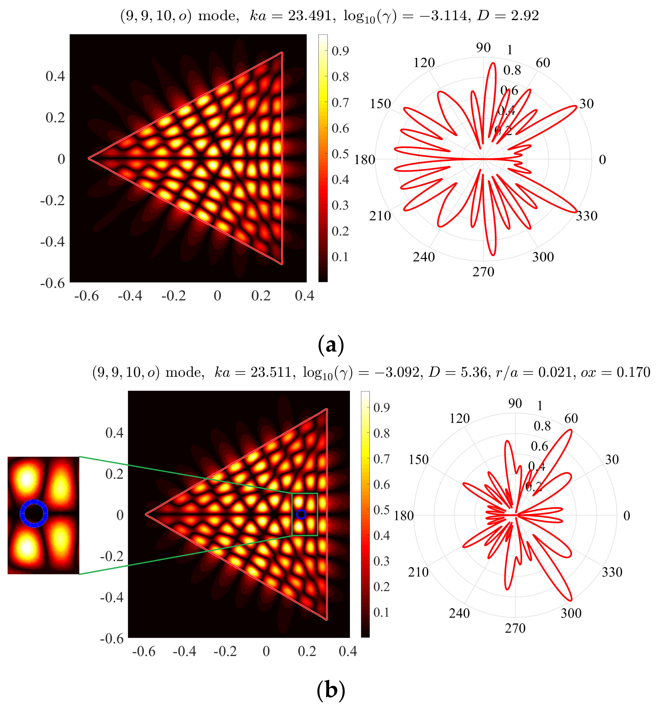
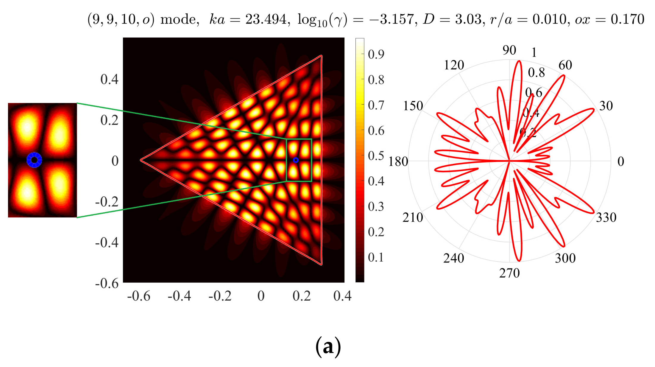
Figure 2a shows near and far fields (i.e., the absolute value of the magnetic field function) of the (9,9,10,o) mode normalized by the maximum value. Here, we use the notation (n1, n2, n3, e) for the even with respect to the x 1 -axis mode. The indices n1, n2, and n3 correspond to the numbers of maxima of the function |u/max(u)| along the upper left-hand side, the lower left-hand side, and the right-hand side of the equilateral triangle, respectively. This mode is one of the two modes, which have minimum thresholds and the normalized frequency of lasing, k a , laying in between 23.5 and 26.5.
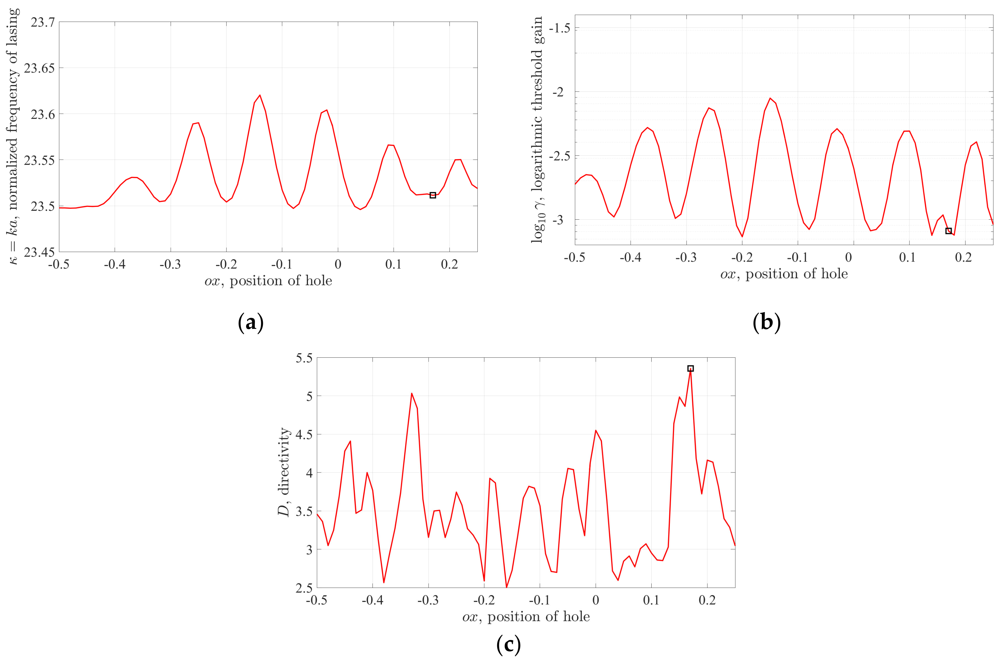
Consider now the same mode of the microcavity of the same shape but with a piercing hole bounded by the circle Γ 1 . At first, we fix the relative radius at r/a = 0.021 and vary the position of the center ( o x , 0 ) of the hole in finite interval, o x 0.5 , 0.25 . The plots of dependences of the frequency of lasing, and the threshold gain index, and the directivity of emission on o x are presented in Figure 3. These plots enable making elementary optimization of the hole position, for the given mode, with either the threshold gain index or the directivity as a target function.
Here, we indicate the values corresponding to the maximum directivity by the hollow squares. This happens at ox = 0.17. Note nearly periodic variations of the studied quantities, with the “period” close to the half-wavelength in the cavity material. Here, the minima (maxima) of the mode threshold gain correspond to the hole position at the nodes (hot spots) of the mode field without the hole. This is because the hole either does not affect or spoils, respectively, the overlap coefficient between the mode electric field and the active region [11].
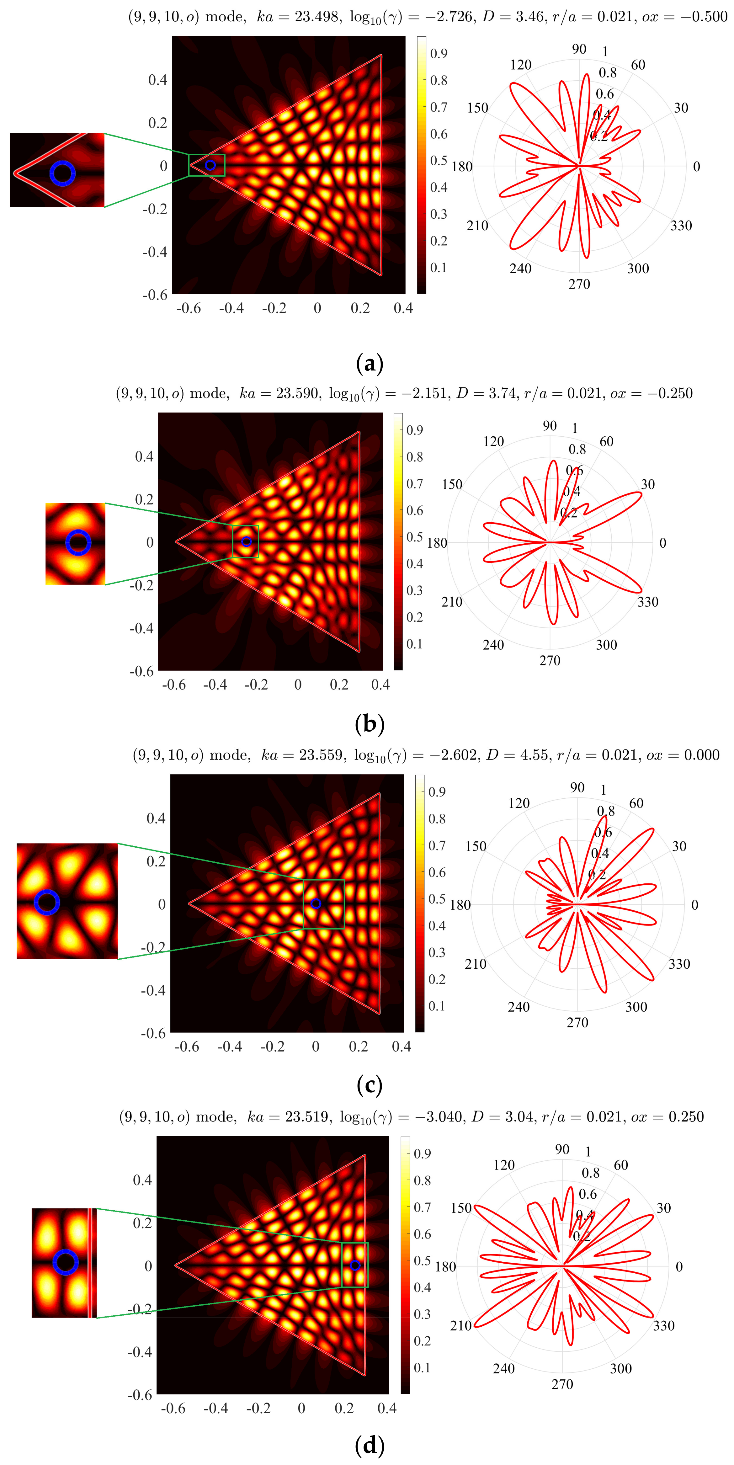
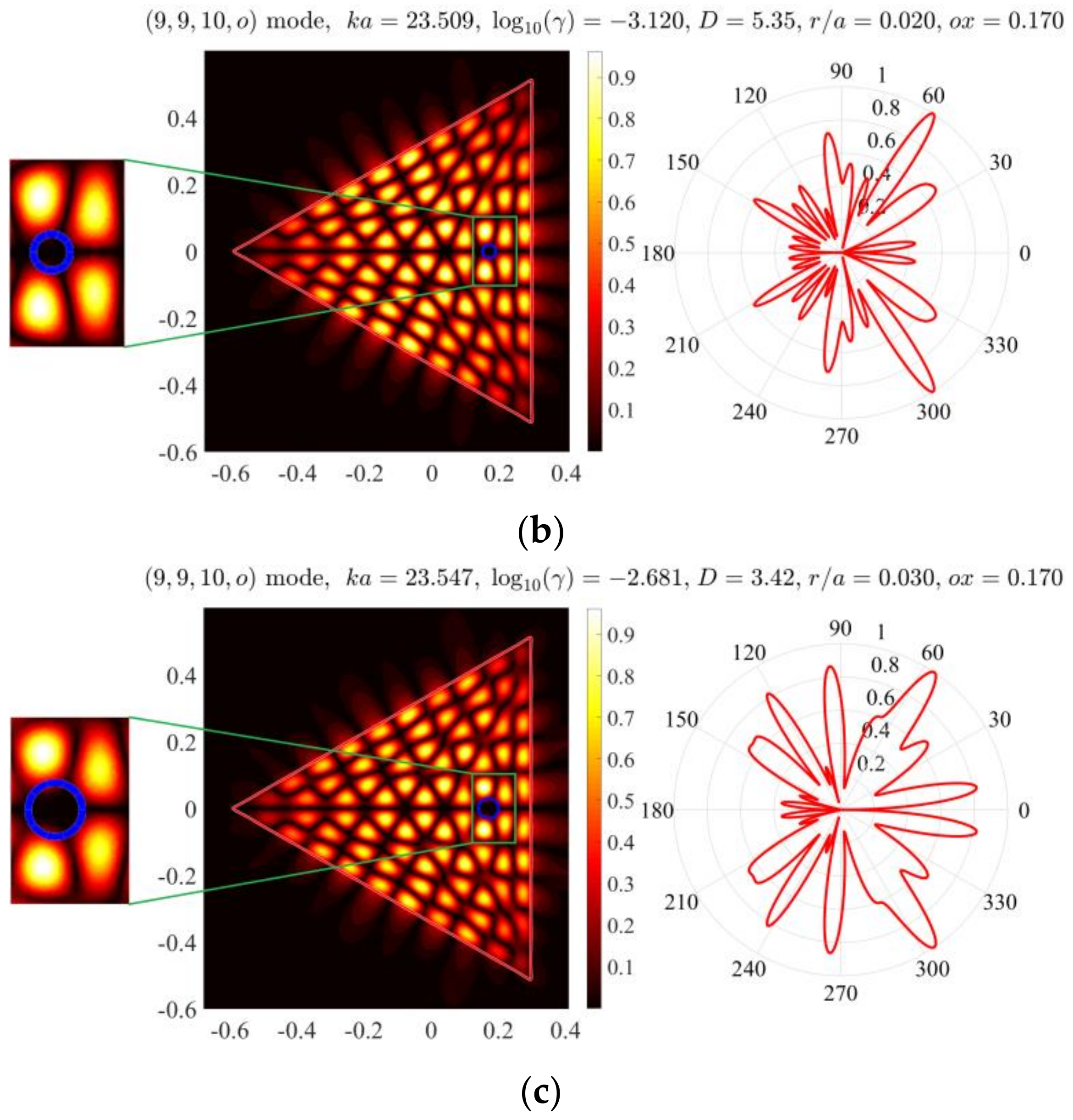
Figure 4 shows the near and far fields of the (9,9,10,o) mode for the same as above triangular microcavity with holes at four different positions on the x-axis.
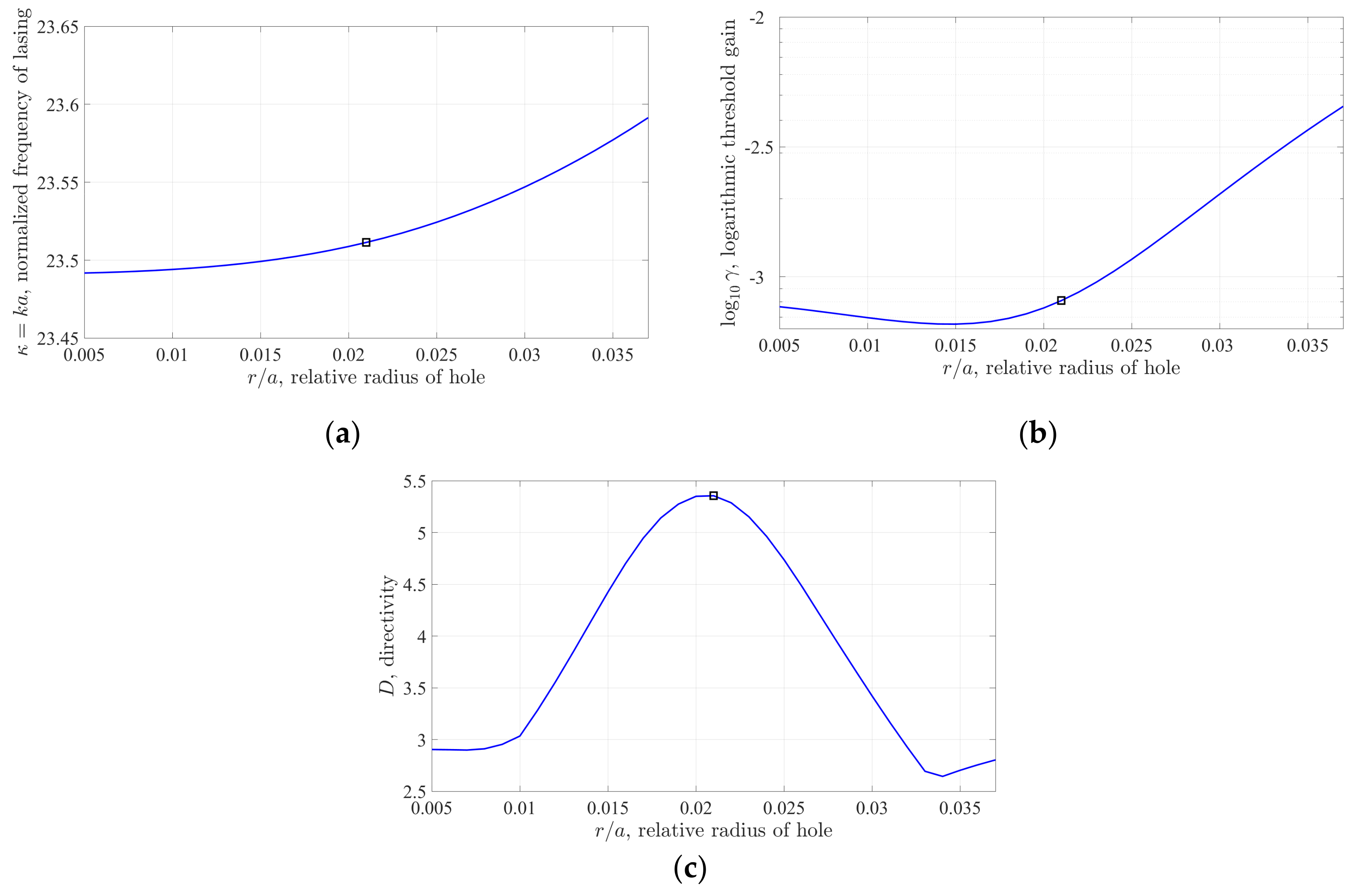
Consider now the same active triangle microcavity with a round hole, the center of which is fixed at the point with the Cartesian coordinates ( 0 , 0.17 ) and suppose that the relative radius of the hole r / a varies between 0.005 and 0.037. The curves in Figure 5 show that for a relatively small hole the emission frequency grows up monotonically (i.e., redshifts) with hole’s radius, in comparison with the frequency of the same mode of the cavity without a hole. The threshold gain index at first goes down slightly and reaches minimum value at r / a = 0.015 . However, if the hole gets larger, so that its diameter approaches half-lambda in the cavity material, then the threshold grows up catastrophically. The directivity D of emission of the analyzed mode varies significantly and reaches a maximum at r / a = 0.021 . In Figure 5, we indicate the values corresponding to this relative radius, by hollow squares. The near and far field patterns in Figure 2b correspond to the optimum hole radius r / a = 0.021 as well to the optimum hole position ox = 0.17. As known, the lasing modes with higher directivities can be useful in many applications.
Finally, for better understanding of the mode characteristics, Figure 6 presents near and far fields of the (9,9,10,o) mode for the triangular microcavity with holes of different radiuses.
As one can see, the hole radius can also be used as a tool of the manipulation of the mode threshold gain and the directivity of emission. Still, it is less efficient than the hole location. An explanation of this fact can be seen in the mode overlap coefficient dependence on these parameters. It is apparently more important to pierce a laser cavity at the proper location (either in the mode electric field minimum or maximum) than to tune it to a certain size. In general, the issue of optimization of mode emission characteristics should be addressed separately for each mode in each specific laser.

5. Conclusions

We have presented the general framework of GCFEP and the main results of its analysis with the aid of the theory of operator-valued functions depending on parameter applying the methods of analytical regularization. We have also linked it to LEP as a full-wave classical electromagnetic theory of laser modes on threshold. Additionally, we highlighted the main steps in the conversion of GFEP and LEP for a 2-D laser with a partial active region to a set of four coupled boundary integral equations of the Muller type. We have further explained the discretization of these equations with the Nystrom quadrature method and proved its convergence. Finally, we have precisely calculated the on-threshold characteristics of a typical lasing mode of a microcavity shaped as an equilateral triangle having a circular piercing hole. In the numerical experiments, we have varied the position of the piercing hole on the x1 axis in the cavity and the radius of the hole and measured the changes in the lasing frequencies, directionalities, and thresholds. Our numerical investigation has shown that a hole of a suitable radius and located at a certain place can lead to a notable growth of the directivity of lasing mode with the conservation of its low threshold. Hence, a small piercing hole’s radius and position in the 2-D equilateral triangular dielectric microcavity laser can be used as an engineering tool to control efficiently the directivity of emission.
We would like to emphasize that the laser model presented here possesses full mathematical rigor for the analysis of the on-threshold laser modes. This is its strength but also its limitation as it is not able to reveal time dynamics of lasing and does not account for the non-linear effects. A lesser limitation can be seen in the assumption that the material gain index in active region does not depend on the wavelength. Note that the way to overcome this limitation has been proposed in [13]. It is necessary to introduce a normalized spectral function of the gain and look for its amplitude coefficient as eigenvalue. This can be seen as a possible direction of future work. Besides, the cavity model can be refined. For instance, it is known that shaping the cavity with the aid of the molecular beam epitaxy results in the “bleaching” [15]. This can be accounted for by introducing a narrow passive region along the cavity rim and the hole rim.
Another direction of research should be the development of a numerical optimization code, based on extremely efficient code for numerical analysis, presented here. Here, a target function should be either the mode threshold gain or the directivity of its emission or a suitable combination of both. For optimization of the laser cavity shape and the active region shape, one can follow, for instance, the guidelines presented in the works [47,48].

Author Contributions

Conceptualization, A.I.N.; methodology, A.O.S., E.M.K. and A.I.N.; software, A.O.S.; validation, A.O.S., E.M.K. and A.I.N.; formal analysis, A.O.S. and E.M.K.; investigation, A.O.S.; writing—original draft preparation, A.O.S., E.M.K., and A.I.N.; writing—review and editing, A.O.S., E.M.K., and A.I.N.; visualization, A.O.S. and A.I.N.

Funding

In this work, A.O.S. was supported, in part, by RFBR via the research project No. 18-31-00026.

Conflicts of Interest

The authors declare no conflict of interest.

References

  1. Yokoyama, H.; Ujihara, K. (Eds.) Spontaneous Emission and Laser Oscillation in Microcavities; CRC Publ.: Roca Baton, FL, USA, 1995. [Google Scholar]
  2. Noeckel, J.U.; Chang, R.K. 2-D microcavities: Theory and experiments. In Cavity-Enhanced Spectroscopies; Van Zee, R.D., Looney, J.P., Eds.; Academic Press: San Diego, CA, USA, 2002. [Google Scholar]
  3. Tureci, H.E.; Stone, A.D. Mode competition and output power in regular and chaotic dielectric cavity lasers. Proc. SPIE 2005, 5708, 255–270. [Google Scholar]
  4. Lebental, M.; Bogomolny, E.; Zyss, J. Organic micro-lasers: A new avenue onto wave chaos physics. In Practical Applications of Microresonators in Optics and Photonics; Matsko, A.B., Ed.; CRC Press: Roca Baton, FL, USA, 2009; pp. 317–353. [Google Scholar]
  5. Cao, H.; Wiersig, J. Dielectric microcavities: Model systems for wave chaos and non-Hermitian physics. Rev. Mod. Phys. 2015, 87, 61–111. [Google Scholar] [CrossRef]
  6. He, L.; Ozdemir, S.K.; Yang, L. Whispering gallery microcavity lasers. Laser Photon. Rev. 2013, 7, 60–82. [Google Scholar] [CrossRef]
  7. Zhang, Y.; Zhang, X.; Li, K.H.; Cheung, Y.F.; Feng, C.; Cho, H.W. Advances in III-nitride semiconductor microdisk lasers. Phys. Status Solidi A 2015, 212, 960–973. [Google Scholar] [CrossRef]
  8. Yang, S.; Wang, Y.; Sun, H. Advances and prospects for whispering gallery mode microcavities. Adv. Opt. Mater. 2015, 3, 1136–1162. [Google Scholar] [CrossRef]
  9. Smotrova, E.I.; Nosich, A.I. Mathematical study of the two-dimensional lasing problem for the whispering-gallery modes in a circular dielectric microcavity. Opt. Quant. Electron. 2004, 36, 213–221. [Google Scholar] [CrossRef]
  10. Smotrova, E.I.; Nosich, A.I.; Benson, T.M.; Sewell, P. Cold-cavity thresholds of microdisks with uniform and non-uniform gain: Quasi-3D modeling with accurate 2D analysis. IEEE J. Sel. Top. Quant. Electron. 2005, 11, 1135–1142. [Google Scholar] [CrossRef]
  11. Smotrova, E.I.; Byelobrov, V.O.; Benson, T.M.; Ctyroky, J.; Sauleau, R.; Nosich, A.I. Optical theorem helps understand thresholds of lasing in microcavities with active regions. IEEE J. Quant. Electron. 2011, 47, 20–30. [Google Scholar] [CrossRef]
  12. Zolotukhina, A.S.; Spiridonov, A.O.; Karchevskii, E.M.; Nosich, A.I. Lasing modes of a microdisk with a ring gain area and of an active microring. Opt. Quant. Electron. 2015, 47, 3883–3891. [Google Scholar] [CrossRef]
  13. Zolotukhina, A.S.; Spiridonov, A.O.; Karchevskii, E.M.; Nosich, A.I. Electromagnetic analysis of optimal pumping of a microdisk laser with a ring electrode. Appl. Phys. B 2017, 123, 32. [Google Scholar] [CrossRef]
  14. Smotrova, E.I.; Nosich, A.I. Thresholds of lasing and modal patterns of a limacon cavity analysed with Muller’s integral equations. In Proceedings of the 11th International Conference on Laser and Fiber-Optical Networks Modeling (LFNM), Kharkov, Ukraine, 5–9 September 2011; pp. 1–3. [Google Scholar]
  15. Spiridonov, A.O.; Karchevskii, E.M.; Benson, T.M.; Nosich, A.I. Why elliptic microcavity lasers emit light on bow-tie-like modes instead of whispering-gallery-like modes. Opt. Commun. 2019, 439, 112–117. [Google Scholar] [CrossRef]
  16. Smotrova, E.I.; Tsvirkun, V.; Gozhyk, I.; Lafargue, C.; Ulysse, C.; Lebental, M.; Nosich, A.I. Spectra, thresholds, and modal fields of a kite-shaped microcavity laser. J. Opt. Soc. Am. B 2013, 30, 1732–1742. [Google Scholar] [CrossRef]
  17. Spiridonov, A.O.; Karchevskii, E.M.; Nosich, A.I. Symmetry accounting in the integral-equation analysis of the lasing eigenvalue problems for two-dimensional optical microcavities. J. Opt. Soc. Am. B 2017, 34, 1435–1443. [Google Scholar] [CrossRef]
  18. Shapoval, O.V.; Kobayashi, K.; Nosich, A.I. Electromagnetic engineering of a single-mode nanolaser on a metal plasmonic strip placed into a circular quantum wire. IEEE J. Sel. Top. Quant. Electron. 2017, 23, 1501609. [Google Scholar] [CrossRef]
  19. Natarov, D.M.; Benson, T.M.; Nosich, A.I. Electromagnetic analysis of the lasing thresholds of hybrid plasmon modes of a silver tube nanolaser with active core and active shell. Beilstein J. Nanotechnol. 2019, 10, 294–304. [Google Scholar] [CrossRef] [PubMed]
  20. Byelobrov, V.O.; Ctyroky, J.; Benson, T.; Sauleau, R.; Altintas, A.; Nosich, A.I. Low-threshold lasing eigenmodes of an infinite periodic chain of quantum wires. Opt. Lett. 2010, 35, 3634–3636. [Google Scholar] [CrossRef] [PubMed]
  21. Byelobrov, V.O.; Benson, T.M.; Nosich, A.I. Binary grating of subwavelength silver and quantum wires as a photonic-plasmonic lasing platform with nanoscale elements. IEEE J. Sel. Top. Quant. Electron. 2012, 18, 1839–1846. [Google Scholar] [CrossRef]
  22. Nezhad, M.P.; Simic, A.; Bondarenko, O.; Slutsky, B.; Mizrahi, A.; Feng, L.; Lomakin, V.; Fainman, Y. Room-temperature subwavelength metallo-dielectric lasers. Nat. Photon. 2010, 4, 395–399. [Google Scholar] [CrossRef]
  23. Mock, A. First principles derivation of microcavity semiconductor laser threshold condition and its application to FDTD active cavity modeling. J. Opt. Soc. Am. B 2010, 27, 2262–2272. [Google Scholar] [CrossRef]
  24. Chang, S.W. Confinement factors and modal volumes of micro- and nanocavities invariant to integration regions. IEEE J. Sel. Top. Quant. Electron. 2012, 18, 1771–1780. [Google Scholar] [CrossRef]
  25. Gagnon, D.; Dumont, J.; Deziel, J.-L.; Dube, L.J. Ab initio investigation of lasing thresholds in photonic molecules. J. Opt. Soc. Am. B 2014, 31, 1867–1873. [Google Scholar] [CrossRef] [Green Version]
  26. Huang, Y.; Lu, Y.Y. Efficient method for lasing eigenvalue problems of periodic structures. J. Mod. Opt. 2014, 61, 390–396. [Google Scholar] [CrossRef]
  27. Spiridonov, A.O.; Karchevskii, E.M.; Nosich, A.I. Rigorous formulation of the lasing eigenvalue problem as a spectral problem for a Fredholm operator function. Lobachevskii J. Math. 2018, 39, 1148–1157. [Google Scholar] [CrossRef]
  28. Djellali, N.; Gozhyk, I.; Owens, D.; Lozenko, S.; Lebental, M.; Lautru, J.; Ulysse, C.; Kippelen, B.; Zyss, J. Controlling the directional emission of holey organic microlasers. Appl. Phys. Lett. 2009, 95, 101108. [Google Scholar] [CrossRef]
  29. Heider, P. Computation of scattering resonances for dielectric resonators. Comput. Math. Appl. 2010, 60, 1620–1632. [Google Scholar] [CrossRef] [Green Version]
  30. Kartchevski, E.M.; Nosich, A.I.; Hanson, G.W. Mathematical analysis of the generalized natural modes of an inhomogeneous optical fiber. SIAM J. Appl. Math. 2005, 65, 2033–2048. [Google Scholar] [CrossRef]
  31. Reichardt, H. Ausstrahlungsbedingungen fur die wellengleihung. Abhandlungen aus dem Mathematischen Seminar der Universitat Hamburg 1960, 24, 41–53. [Google Scholar]
  32. Colton, D.; Kress, R. Integral Equation Methods in Scattering Theory; Society for Industrial and Applied Mathematics: Philadelphia, PA, USA, 2013. [Google Scholar]
  33. Karchevskii, E.; Nosich, A. Methods of analytical regularization in the spectral theory of open waveguides. In Proceedings of the International Conference on Mathematical Methods in Electromagnetic Theory (MMET*2014), Dnipro, Ukraine, 26–28 August 2014; pp. 39–45. [Google Scholar]
  34. Nosich, A.I. Method of analytical regularization in computational photonics. Radio Sci. 2016, 51, 1421–1430. [Google Scholar] [CrossRef]
  35. Muller, C. Mathematical Foundations of the Electromagnetic Waves; Springer: Berlin, Germany, 1969. [Google Scholar]
  36. Kress, R. Linear Integral Equations; Springer Monographs in Mathematics; Springer: New York, NY, USA, 1999. [Google Scholar]
  37. Seeley, R. Integral equations depending analytically on a parameter. Indag. Math. 1964, 24, 434–442. [Google Scholar]
  38. Kozlov, V.; Maz’ya, V. Differential Equations with Operator Coefficients; Springer Monographs in Mathematics; Springer: Berlin/Heidelberg, Germany, 1999. [Google Scholar]
  39. Bonnet-Ben Dhia, A.-S.; Durufle, M.; Joly, P.; Joubert, L. Stability of acoustic propagation in 2D duct flows: A low frequency approach. Math. Models Methods Appl. Sci. 2011, 21, 1121–1151. [Google Scholar] [CrossRef]
  40. Steinberg, S. Meromorphic families of compact operators. Arch. Ration. Mech. Anal. 1968, 31, 372–379. [Google Scholar] [CrossRef]
  41. Colton, D.; Kress, R. Inverse Acoustic and Electromagnetic Scattering Theory; Springer: Berlin/Heidelberg, Germany, 1998. [Google Scholar]
  42. Karma, O. Approximation in eigenvalue problems for holomorphic Fredholm operator functions i. Numer. Funct. Anal. Optim. 1996, 17, 365–387. [Google Scholar] [CrossRef]
  43. Yang, Y.-D.; Huang, Y.-Z.; Wang, S.-J. Mode analysis for equilateral-triangle-resonator microlasers with metal confinement layers. IEEE J. Quant. Electron. 2009, 45, 1529–1536. [Google Scholar] [CrossRef]
  44. Sukharevsky, I.O.; Nosich, A.I.; Altintas, A. Manipulation of backscattering from a dielectric cylinder of triangular cross-section using the interplay of GO-like ray effects and resonances. IEEE Trans. Antennas Propagat. 2015, 63, 2162–2169. [Google Scholar] [CrossRef]
  45. Sukharevsky, I.O.; Lebental, M.; Dietzc, B.; Lafargue, C.; Bittner, S. Dielectric equilateral triangle microresonators: Integral equations and semiclassical physics approaches. Proc. SPIE 2018, 10518, 105181U. [Google Scholar] [CrossRef]
  46. Bickley, W.G. Two-dimension potential problems concerning a single closed boundary. Phil. Trans. 1929, 228, 235–273. [Google Scholar] [CrossRef]
  47. Ning, J.; Liang, S.Y. Inverse identification of Johnson-Cook material constants based on modified chip formation model and iterative gradient search using temperature and force measurements. Int. J. Adv. Manuf. Technol. 2019, 102, 2865–2876. [Google Scholar] [CrossRef]
  48. Ning, J.; Nguyen, V.; Huang, Y.; Hartwig, K.T.; Liang, S.Y. Inverse determination of Johnson–Cook model constants of ultra-fine-grained titanium based on chip formation model and iterative gradient search. Int. J. Adv. Manuf. Technol. 2018, 99, 1131–1140. [Google Scholar] [CrossRef]
Figure 1. Geometry of a 2-D optical resonator with a piercing hole.
Axioms 08 00101 g001
Figure 2. Normalized near and far field patterns of the mode (9,9,10,o) of the fully active triangular microcavity laser (a). Panel (b) shows the near and far fields of the same mode with the hole position and the hole radius providing the maximum D. A zoom of the vicinity of the hole is also shown.
Axioms 08 00101 g002
Figure 3. Dependence of the normalized frequency (a), threshold gain index (b), and directivity of emission (c) of the mode (9,9,10,o) on the normalized position of the hole on the x-axis, x/a. Relative radius of the hole is r/a = 0.021.
Axioms 08 00101 g003
Figure 4. Near and far fields of the mode (9,9,10,o) of the cavity with the hole, r/a = 0.021 and ox = −0.5 (a), −0.25 (b), 0 (c), and 0.25 (d).
Axioms 08 00101 g004
Figure 5. Dependence of the normalized frequency (a), threshold gain index (b), and directivity of emission (c) of the mode (9,9,10,o) on the relative radius of the hole located at (0, 0.17).
Axioms 08 00101 g005
Figure 6. Normalized near and far fields of the mode (9,9,10,o) of the cavity with the hole, r/a = 0.01 (a), 0.02 (b), 0.03 (c), ox = 0.17.
Axioms 08 00101 g006aAxioms 08 00101 g006b

