An Efficient Class of Traub–Steffensen-Type Methods for Computing Multiple Zeros

Abstract

Numerous higher-order methods with derivative evaluations are accessible in the literature for computing multiple zeros. However, higher-order methods without derivatives are very rare for multiple zeros. Encouraged by this fact, we present a family of third-order derivative-free iterative methods for multiple zeros that require only evaluations of three functions per iteration. Convergence of the proposed class is demonstrated by means of using a graphical tool, namely basins of attraction. Applicability of the methods is demonstrated through numerical experimentation on different functions that illustrates the efficient behavior. Comparison of numerical results shows that the presented iterative methods are good competitors to the existing techniques.

1. Introduction

We consider derivative-free methods to discover a multiple root (say, $\alpha$) of multiplicity m, i.e., $f^{\left(r\right)}\left(\alpha \right)=0,r=0,1,2,\dots ,m-1$ and $f^{\left(m\right)}\left(\alpha \right)\ne 0$, of a nonlinear equation $f\left(x\right)=0$.

Many higher-order methods, either independent or based on the modified Newton’s method [1] with quadratically convergent

$$x_{n+1}=x_n-m\frac{f\left(x_n\right)}{f^{\prime }\left(x_n\right)},$$

(1)

have been proposed and verified in the literature; see, for example: [2,3,4,5,6,7,8,9,10,11,12,13,14,15] and references therein. Such methods require the evaluations of derivatives of either linear order or linear and second order, or both. However, higher-order derivative-free methods to handle the case of multiple roots are yet to be explored. The main reason for the non-availability of such methods is due to the difficulty in obtaining their order of convergence. The derivative-free methods are important in the conditions when derivative of the function f is difficult to compute or is expensive to obtain. One such method free from derivative is the classical Traub–Steffensen method [16] which actually replaces the derivative $f^{\prime }$ in the classical Newton method with appropriate approximation based on difference quotient,

$$f^{\prime }\left(x_n\right)\simeq \frac{f(x_n+\beta f\left(x_n\right))-f\left(x_n\right)}{\beta f\left(x_n\right)},\beta \in \mathbb{R}-\left\{0\right\},$$

or

$$f^{\prime }\left(x_n\right)\simeq f[x_n,w_n],$$

where $w_n=x_n+\beta f\left(x_n\right)$ and $f[x_n,w_n]=\frac{f\left(w_n\right)-f\left(x_n\right)}{w_n-x_n}$ is a first-order divided difference.

In this way the modified Newton method (1) becomes the modified Traub–Steffensen method

$$x_{n+1}=x_n-m\frac{f\left(x_n\right)}{f[x_n,w_n]}.$$

(2)

The modified Traub–Steffensen method (2) is a noteworthy improvement of Newton’s method, because it keeps quadratic convergence without using derivative.

In this work, we introduce a two-step family of third-order derivative-free methods for computing multiple zeros that require three evaluations of the function f per iteration. The iterative scheme uses the Traub–Steffensen iteration (2) in the first step and Traub–Steffensen-like iteration in the second step. The procedure is based on a simple approach of using weight factors in the iterative scheme. Many special methods of the family can be generated depending on the forms of weight factors. Efficacy of these methods is tested on various numerical problems of different natures. In the comparison with existing techniques that use derivative evaluations, the new derivative-free methods are computationally more efficient.

The rest of the paper is summarized as follows. In Section 2, the scheme of third-order methods is developed and its convergence is studied. Section 3 is divided into two parts: Section 3.1 and Section 3.2. In Section 3.1, an initial approach concerning the study of the dynamics of the methods with the help of basins of attraction is presented. To demonstrate applicability and efficacy of the new methods, some numerical experiments are performed in Section 3.2. A comparison of the methods with existing ones of the same order is also shown in this subsection. Concluding remarks are given in Section 4.

2. The Method

With a known multiplicity $m\ge 1$, we consider the following two-step scheme for multiple roots based on the Traub–Steffensen method (2)

$$\left\{\begin{array}{c}{y}_n=x_n-m\frac{f\left(x_n\right)}{f[x_n,w_n]},\hfill \\ x_{n+1}=y_n-H\left(u\right)\frac{f\left(x_n\right)}{f[x_n,w_n]},\hfill \end{array}\right.$$

(3)

where the function $H\left(u\right):\mathbb{C}\to \mathbb{C}$ is analytic in a neighborhood of ‘0’ with $u={\left(\frac{f\left(y_n\right)}{f\left(x_n\right)}\right)}^{\frac{1}{m}}$. The convergence order is obtained by the following theorem:

Theorem 1.

Let $f:\mathbb{C}\to \mathbb{C}$ be an analytic function in a region enclosing a multiple zero (say, α) with multiplicity m. Assume that initial approximation $x_0$ is sufficiently close to α, then the iteration scheme defined by (3) has attained third order of convergence, provided that $H\left(0\right)=0$ and $H^{\prime }\left(0\right)=m$.

Proof. 

Let the error at n-th iteration be $e_n=x_n-\alpha$. Using Taylor’s expansion of $f\left(x_n\right)$ about $\alpha$, we have that

$$f\left(x_n\right)=\frac{f^{\left(m\right)}\left(\alpha \right)}{m!}{e}_n^m\left(1+C_1{e}_n+C_2{e}_n^2+C_3{e}_n^3+O({\left(e_n\right)}^4)\right),$$

(4)

where $C_k=\frac{m!}{(m+k)!}\frac{f^{(m+k)}\left(\alpha \right)}{f^{\left(m\right)}\left(\alpha \right)}$ for $k\in \mathbb{N}$.

Also

$$\begin{array}{cc}\hfill w_n-\alpha =& x_n-\alpha +\beta f\left(x_n\right)\hfill \\ \hfill =& e_n(1+\frac{\beta f^{\left(m\right)}\left(\alpha \right)}{m!}{e}_n^{m-1})+\frac{\beta f^{\left(m\right)}\left(\alpha \right)}{m!}{e}_n^m\left(C_1{e}_n+C_2{e}_n^2+C_3{e}_n^3+O({\left(e_n\right)}^4)\right).\hfill \end{array}$$

Then Taylor’s expansion of $f\left(w_n\right)$ about $\alpha$ is given as

$$f\left(w_n\right)=\frac{f^{\left(m\right)}\left(\alpha \right)}{m!}{(w_n-\alpha )}^m\left(1+C_1(w_n-\alpha )+C_2(w_n-\alpha )+C_3(w_n-\alpha )+O({(w_n-\alpha )}^4)\right),$$

(5)

By using (4) and (5), then the first step of the scheme (3) yields

$$y_n-\alpha =\frac{C_1\beta }{m}{e}_n^2-\frac{{\beta }^2}{m^2}\left((m+1)C_1^2-2m{C}_2\right)e_n^3+O({\left(e_n\right)}^4)).$$

(6)

Expansion of $f\left(y_n\right)$ about $\alpha$ leads us to the expression

$$\begin{array}{cc}\hfill f\left(y_n\right)=& \frac{f^{\left(m\right)}\left(\alpha \right)}{m!}{\left(\frac{\beta C_1}{m}\right)}^m{e}_n^{2m}(1-\frac{\beta X_1}{C_1}{e}_n+\frac{\beta }{2m{C}_1^2}\left(\beta (m-1)X_1^2+2C_1^4\right)e_n^2\hfill \\ & -\frac{\beta X_1}{6m^2{C}_1^3}\left(6\beta C_1^4(m+1)+{\beta }^2(m-1)(m-2)X_1^2\right)e_n^3)+O\left(\left(e_n^4\right)\right),\hfill \end{array}$$

(7)

where $X_1=(m+1)C_1^2-2m{C}_2$.

Expanding $H\left(u\right)$ in the neighborhood of ‘0’, then using (4) and (7) in the expansion of $u={\left(\frac{f\left(y_n\right)}{f\left(x_n\right)}\right)}^{\frac{1}{m}}$, we have

$$\begin{array}{cc}\hfill H\left(u\right)=& H\left(0\right)+H^{\prime }\left(0\right)\left(\frac{C_1\beta }{m}{e}_n-\frac{\beta }{m^2}(\beta X_1+C_1^2)e_n^2+\frac{\beta C_1}{2m^3}\left((2\beta +1)X_1+2C_1^2\right)\right)e_n^3+O({\left(e_n\right)}^4).\hfill \end{array}$$

(8)

Using the above expressions in the last step of (3), it follows that

$$\begin{array}{cc}\hfill e_{n+1}=& -\frac{H\left(0\right)}{m}{e}_n+\frac{\beta C_1}{m^2}\left(m+H\left(0\right)-H^{\prime }\left(0\right)\right)e_n^2-\frac{1}{m^3}({\beta }^2\left((1+m)C_1^2+2C_2\right)\left(m+H\left(0\right)+H^{\prime }\left(0\right)\right)\hfill \\ & -2\beta C_1^2{H}^{\prime }\left(0\right))e_n^3+O({\left(e_n\right)}^4).\hfill \end{array}$$

(9)

It is clear that the third order of convergence is possible only if $H\left(0\right)=0,H^{\prime }\left(0\right)=m$. Then, the error Equation (9) becomes

$$e_{n+1}=\frac{2\beta C_1^2}{m^2}{e}_n^3+O({\left(e_n\right)}^4).$$

Thus, the theorem is proved. □

Some Concrete Forms of H(u)

We can obtain numerous methods of the family (3) based on the form of function $H\left(u\right)$ that satisfies the conditions of Theorem 1. but we will limit choices to consider the forms of low-order polynomials or simple functions. Accordingly, the following simple forms are chosen:

(1)

$H\left(u\right)=mu$,

(2)

$H\left(u\right)=\frac{mu}{1+u},$

(3)

$H\left(u\right)=\frac{mu}{1-u}$,

(4)

$H\left(u\right)=\frac{mu}{1+mu},$

(5)

$H\left(u\right)=mlog(u+1)$,

(6)

$H\left(u\right)=m(e^u-1).$

The corresponding method for each of the above forms can be expressed as:

• Method 1 (M1):

  $$x_{n+1}=y_n-mu\frac{f\left(x_n\right)}{f[x_n,w_n]}.$$
• Method 2 (M2):

  $$x_{n+1}=y_n-\frac{mu}{1+u}\frac{f\left(x_n\right)}{f[x_n,w_n]}.$$
• Method 3 (M3):

  $$x_{n+1}=y_n-\frac{mu}{1-u}\frac{f\left(x_n\right)}{f[x_n,w_n]}.$$
• Method 4 (M4):

  $$x_{n+1}=y_n-\frac{mu}{1+mu}\frac{f\left(x_n\right)}{f[x_n,w_n]}.$$
• Method 5 (M5):

  $$x_{n+1}=y_n-mlog(u+1)\frac{f\left(x_n\right)}{f[x_n,w_n]}.$$
• Method 6 (M6):

  $$x_{n+1}=y_n-m(e^u-1)\frac{f\left(x_n\right)}{f[x_n,w_n]}.$$

In the above each case $u={\left(\frac{f\left(y_n\right)}{f\left(x_n\right)}\right)}^{\frac{1}{m}}$ and $y_n=x_n-m\frac{f\left(x_n\right)}{f[x_n,w_n]}$.

Remark 1.

Computational competence of an iterative method is spanned by the efficiency index $E=s^{1/d}$ (see [17]), where s is the order of convergence and d is the computational cost measured as the number of new pieces of information needed by the method per iterative step. A “piece of information” typically is any calculation of the function f or one of its derivatives. The presented third-order methods require three function calculations per iteration, so the efficiency index of the methods is $E=\sqrt[3]{3}\approx 1.442$ which is equal to the efficiency index of existing third-order methods such as Dong [5], Halley [7], Chebyshev [7], Osada [12], and Victory and Neta [14]. Note, however, that these existing third-order methods require derivative evaluations in their computation which is not the case with the proposed methods. Also note that efficiency index of new methods is better than that of modified Newton’s method and derivative-free Traub–Steffensen’s method $(E=\sqrt{2}\approx 1.414)$.

3. Numerical Tests

In this section, first we plot the basins of attraction of the zeros of some polynomials when the proposed iterative methods are applied on the polynomials. Next, we verify the theoretical results by the applications of the methods on some nonlinear functions, including those which arise in practical problems.

3.1. Basins of Attraction

Analysis of the complex dynamical behavior gives important information about convergence and stability of an iterative scheme; see e.g., [2,3,18,19,20,21]. Here, we directly describe the dynamics of iterative methods M1–M6 by means of visual display of the basins of attraction of the zeros of a polynomial $P\left(z\right)\in \mathbb{C}$. The deep dynamical study of the proposed six methods, with a detailed stability analysis of the fixed points and their behavior, requires a separate article, and so such complete analysis is not a subject of discussion in the present work.

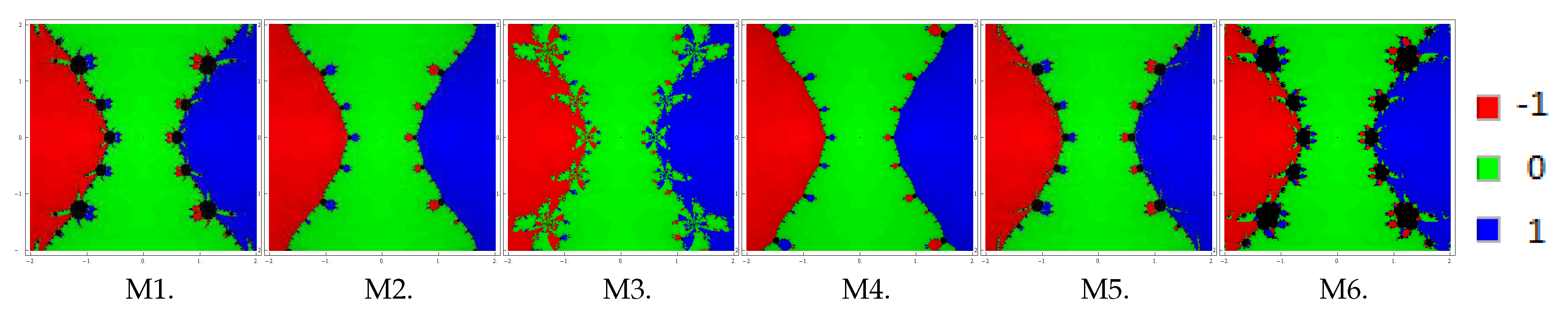
To start with, let us take the initial point $z_0$ in a rectangular region $R\in \mathbb{C}$ that contains all the zeros of a polynomial $P\left(z\right).$ The iterative method starts from point $z_0$ in a rectangle either converges to the zero $P\left(z\right)$ or eventually diverges. The stopping criterion for convergence is considered to be ${10}^{-3}$ up to a maximum of 25 iterations. If the required tolerance is not achieved in 25 iterations, we conclude that the method starting at point $z_0$ does not converge to any root. The strategy adopted is as follows: A color is allocated to each initial point $z_0$ in the basin of attraction of a zero. If the iteration initiating at $z_0$ converges, then it represents the attraction basin with that particular assigned color to it, otherwise if it fails to converge in 25 iterations, then it shows the black color.

We plot the basins of attraction of the methods M1–M6 (for the choices $\beta ={10}^{-2},{10}^{-4},{10}^{-6}$) on following three polynomials:

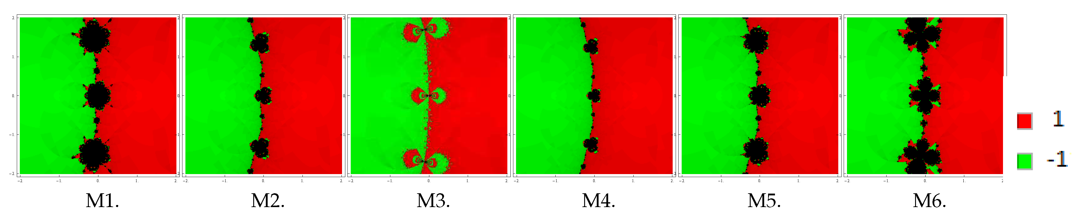
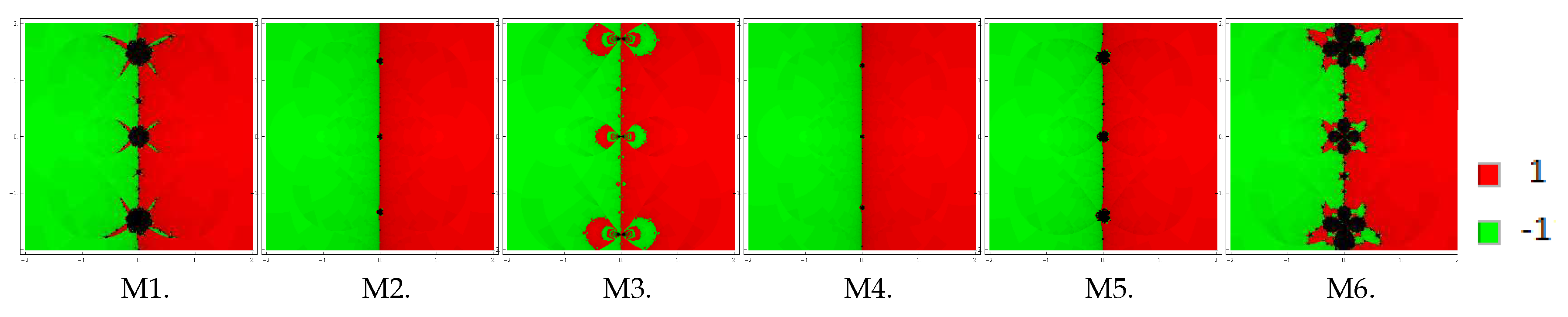
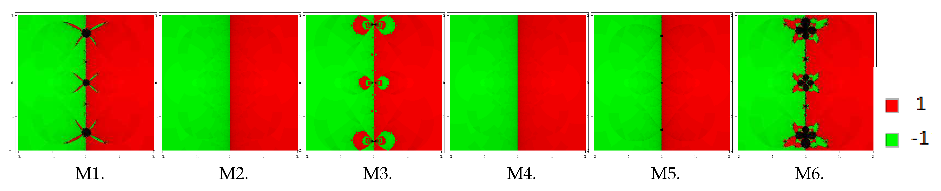
Problem 1.

In the first example, we look at the polynomial $P_1\left(z\right)={(z^2-1)}^2$ which has zeros $\{\pm 1\}$ with multiplicity 2. For making basins, we use a grid of $400\times 400$ points in a rectangle $D\in \mathbb{C}$ of size $[-2,2]\times [-2,2]$ and fix the color green to each initial point in the basin of attraction of zero ‘$-1$’ and the color red to each point in the basin of attraction of zero ‘1’. 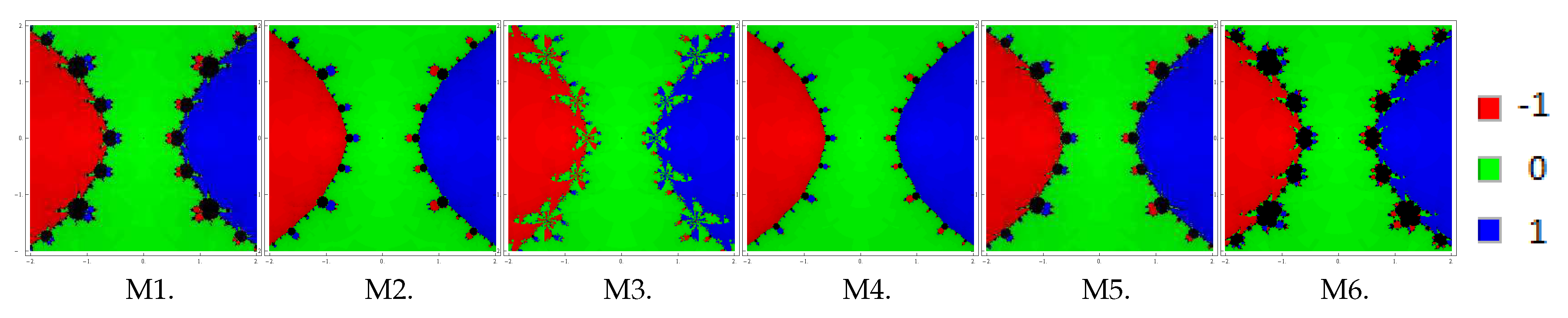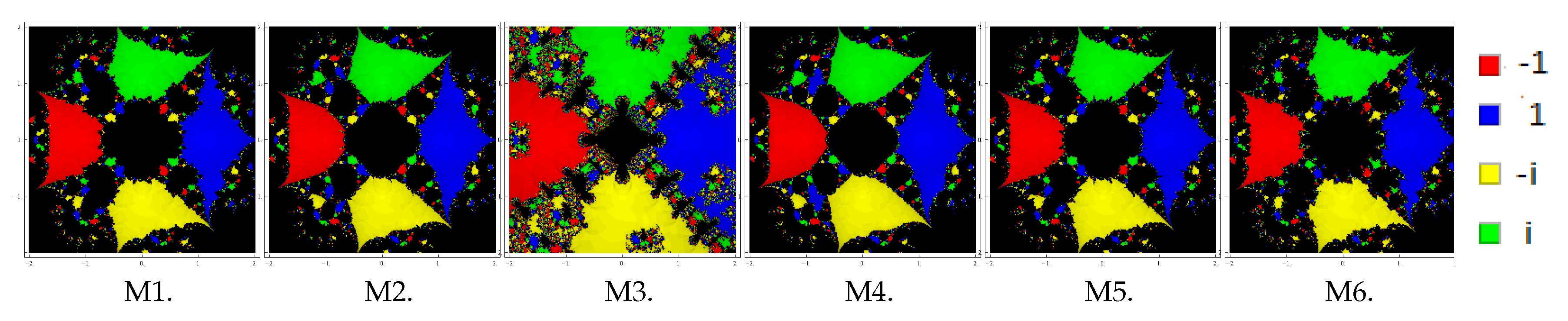Basins achieved for the methods M1–M6 are shown in Figure 1, Figure 2 and Figure 3 corresponding to $\beta ={10}^{-2},{10}^{-4},{10}^{-6}$. Looking at the behavior of the methods, we see that methods M2 and M4 possess fewest divergent points, followed by M3 and M5. On the contrary, the method M6 has the most divergent points, followed by M1. Notice that the basins are becoming better as parameter β assumes smaller values.

Problem 2.

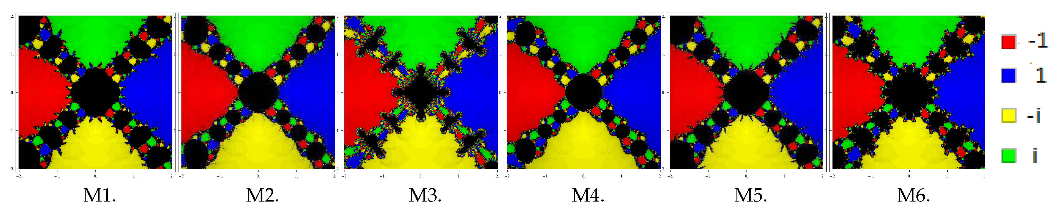
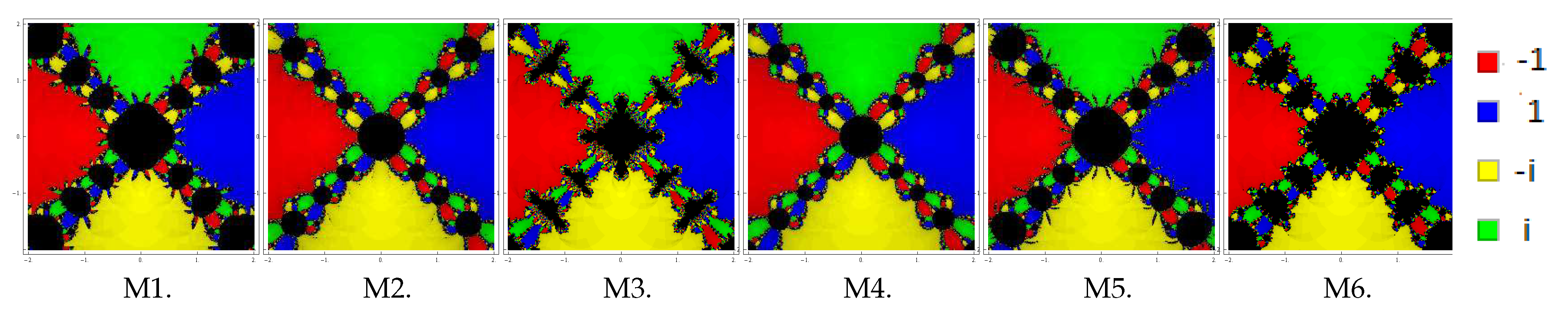
Let us consider the polynomial $P_2\left(z\right)={(z^3-z)}^3$ with zeros $\{0,\pm 1\}$ with multiplicity 3. To examine the dynamical view, we consider a rectangle $D=[-2,2]\times [-2,2]\in \mathbb{C}$ with $400\times 400$ grid points and allot the colors red, green, and blue to each point in the basin of attraction of $-1$, 0 and 1, respectively. Basins of this problem are shown in Figure 4, Figure 5 and Figure 6 corresponding to parameter choices $\beta ={10}^{-2},{10}^{-4},{10}^{-6}$ in the proposed methods. Observing the behavior of the methods, we see that methods M3, M2, and M4 have better convergence behavior since they have the least number of divergent points. On the other hand, M6 contains large black regions followed by M1 and M5, indicating that the methods do not converge in 25 iterations starting at those points. Also, observe that the basins are improving with the smaller values of β.

Problem 3.

Lastly, we consider the polynomial $P_3\left(z\right)={(z^4-1)}^2$ with zeros $\{\pm i,\pm 1\}$ with multiplicity 2. To see the dynamical view, we consider a rectangle $D=[-2,2]\times [-2,2]\in \mathbb{C}$ with $400\times 400$ grid points and allocate the colors red, blue, yellow, and green to each point in the basin of attraction of $-1$, 1, $-i$ and i, respectively. Basins for this problem are shown in Figure 7, Figure 8 and Figure 9 corresponding to parameter choices $\beta ={10}^{-2},{10}^{-4},{10}^{-6}$ in the proposed methods. Observing the behavior of the methods, we see that methods M3, M2, and M4 have better convergence behavior since they have fewest divergent points. On the other hand, M6 contains large black regions followed by M1 and M5 indicating that the methods do not converge in 25 iterations starting at those points. Also, observe that the basins are becoming larger with the smaller values of β.

From these graphics, one can easily evaluate the behavior and stability of any method. If we choose an initial point $z_0$ in a zone where distinct basins of attraction touch each other, it is impractical to predict which root is going to be attained by the iterative method that starts in $z_0$. Hence, the choice of $z_0$ in such a zone is not a good one. Both the black zones and the regions with different colors are not suitable to take the initial guess $z_0$ when we want to acquire a unique root. The most adorable pictures appear when we have very tricky frontiers between basins of attraction, and they correspond to the cases where the method is more demanding with respect to the initial point and its dynamic behavior is more unpredictable. We conclude this section with a remark that the convergence nature of proposed methods depends upon the value of parameter $\beta$. The smaller the value of $\beta$, the better the convergence of the method.

3.2. Applications

The above six methods M1–M6 of family (3) are applied to solve a few nonlinear equations, which not only depict the methods practically but also serve to verify the validity of theoretical results we have derived. To investigate the theoretical order of convergence, we obtain the computational order of convergence (COC) using the formula (see [22])

$$COC=\frac{ln|(x_{n+1}-\alpha )/(x_n-\alpha )|}{ln|(x_n-\alpha )/(x_{n-1}-\alpha )|}.$$

Performance is compared with some well-known third-order methods requiring derivative evaluations such as Dong [5], Halley [7], Chebyshev [7], Osada [12], and Victory and Neta [14]. These methods are expressed as:

• Dong’s method (DM):

  $$\left\{\begin{array}{c}{y}_n=x_n-\sqrt{m}\frac{f\left(x_n\right)}{f^{\prime }\left(x_n\right)},\hfill \\ x_{n+1}=y_n-m{\left(1-\frac{1}{\sqrt{m}}\right)}^{1-m}\frac{f\left(y_n\right)}{f^{\prime }\left(x_n\right)}.\hfill \end{array}\right.$$
• Halley’s method (HM):

  $$x_{n+1}=x_n-\frac{f\left(x_n\right)}{\frac{m+1}{2m}{f}^{\prime }\left(x_n\right)-\frac{f\left(x_n\right)f^{″}\left(x_n\right)}{2f^{\prime }\left(x_n\right)}}.$$
• Chebyshev’s method (CM):

  $$x_{n+1}=x_n-\frac{m(3-m)}{2}\frac{f\left(x_n\right)}{f^{\prime }\left(x_n\right)}-\frac{m^2}{2}\frac{f^2\left(x_n\right)f^{″}\left(x_n\right)}{f^{\prime 3}\left(x_n\right)}.$$
• Osada’s method (OM):

  $$x_{n+1}=x_n-\frac{1}{2}m(m+1)\frac{f\left(x_n\right)}{f^{\prime }(x_n}+\frac{1}{2}{(m-1)}^2\frac{f^{\prime }\left(x_n\right)}{f^{″}\left(x_n\right)}.$$
• Victory-Neta method (VNM):

  $$\left\{\begin{array}{c}{y}_n=x_n-\frac{f\left(x_n\right)}{f^{\prime }\left(x_n\right)},\hfill \\ x_{n+1}=y_n-\frac{f\left(y_n\right)}{f^{\prime }\left(x_n\right)}\frac{f\left(x_n\right)+Af\left(y_n\right)}{f\left(x_n\right)+Bf\left(y_n\right)},\hfill \end{array}\right.$$

  where

  $$A={\mu }^{2m}-{\mu }^{m+1},B=-\frac{{\mu }^m(m-2)(m-1)+1}{{(m-1)}^2}\mathrm{and}\mu =\frac{m}{m-1}.$$

All computations are determined in the programming package Mathematica using multiple-precision arithmetic. Performance of the new methods is tested by choosing value of the parameter $\beta =-0.01$. Numerical results displayed in

Table 1. Comparison of performance of methods for Example 1.

Methods	$|{\mathit{x}}_3-{\mathit{x}}_2|$	$|{\mathit{x}}_4-{\mathit{x}}_3|$	$|{\mathit{x}}_5-{\mathit{x}}_4|$	n	COC	CPU-Time
$\mathrm{DM}$	$9.90\times {10}^{-11}$	$1.52\times {10}^{-31}$	$5.49\times {10}^{-94}$	5	3.0000	0.01942
$\mathrm{HM}$	$5.84\times {10}^{-10}$	$4.61\times {10}^{-29}$	$2.24\times {10}^{-86}$	5	3.0000	0.01950
$\mathrm{CM}$	$9.54\times {10}^{-10}$	$2.47\times {10}^{-28}$	$4.30\times {10}^{-84}$	5	3.0000	0.01885
$\mathrm{OM}$	$1.26\times {10}^{-9}$	$6.52\times {10}^{-28}$	$8.94\times {10}^{-83}$	5	3.0000	0.01955
$\mathrm{VNM}$	$2.50\times {10}^{-10}$	$2.92\times {10}^{-30}$	$4.68\times {10}^{-90}$	5	3.0000	0.02250
$\mathrm{M}1$	$1.51\times {10}^{-12}$	$3.91\times {10}^{-37}$	0	4	3.0000	0.00775
$\mathrm{M}2$	$5.15\times {10}^{-12}$	$2.30\times {10}^{-35}$	0	4	3.0000	0.01165
$\mathrm{M}3$	$2.32\times {10}^{-13}$	$7.01\times {10}^{-40}$	0	4	3.0000	0.01175
$\mathrm{M}4$	$4.73\times {10}^{-11}$	$3.59\times {10}^{-32}$	$1.57\times {10}^{-95}$	5	3.0000	0.01285
$\mathrm{M}5$	$2.94\times {10}^{-12}$	$3.57\times {10}^{-36}$	0	4	3.0000	0.01775
$\mathrm{M}6$	$6.71\times {10}^{-13}$	$2.55\times {10}^{-38}$	0	4	3.0000	0.01115

,

Table 2. Comparison of performance of methods for Example 2.

Methods	$|{\mathit{x}}_3-{\mathit{x}}_2|$	$|{\mathit{x}}_4-{\mathit{x}}_3|$	$|{\mathit{x}}_5-{\mathit{x}}_4|$	n	COC	CPU-Time
$\mathrm{DM}$	$6.14\times {10}^{-9}$	$1.48\times {10}^{-26}$	$2.06\times {10}^{-79}$	5	3.0000	0.17575
$\mathrm{HM}$	$5.10\times {10}^{-8}$	$1.20\times {10}^{-23}$	$1.54\times {10}^{-70}$	5	3.0000	0.20354
$\mathrm{CM}$	$5.98\times {10}^{-8}$	$2.17\times {10}^{-23}$	$1.04\times {10}^{-69}$	5	3.0000	0.23560
$\mathrm{OM}$	$6.30\times {10}^{-8}$	$2.63\times {10}^{-23}$	$1.91\times {10}^{-69}$	5	3.0000	0.23225
$\mathrm{VNM}$	$2.45\times {10}^{-8}$	$1.17\times {10}^{-24}$	$1.28\times {10}^{-73}$	5	3.0000	0.24875
$\mathrm{M}1$	$1.28\times {10}^{-15}$	$4.70\times {10}^{-47}$	0	4	3.0000	0.11121
$\mathrm{M}2$	$2.95\times {10}^{-15}$	$8.62\times {10}^{-46}$	0	4	3.0000	0.12100
$\mathrm{M}3$	$3.86\times {10}^{-16}$	$6.45\times {10}^{-49}$	0	4	3.0000	0.10925
$\mathrm{M}4$	$4.96\times {10}^{-14}$	$1.23\times {10}^{-41}$	0	4	3.0000	0.11725
$\mathrm{M}5$	$2.00\times {10}^{-15}$	$2.24\times {10}^{-46}$	0	4	3.0000	0.12125
$\mathrm{M}6$	$7.54\times {10}^{-16}$	$7.21\times {10}^{-48}$	0	4	3.0000	0.12525

,

Table 3. Comparison of performance of methods for Example 3.

Methods	$|{\mathit{x}}_3-{\mathit{x}}_2|$	$|{\mathit{x}}_4-{\mathit{x}}_3|$	$|{\mathit{x}}_5-{\mathit{x}}_4|$	n	COC	CPU-Time
$\mathrm{DM}$	$1.02\times {10}^{-9}$	$3.43\times {10}^{-29}$	$1.31\times {10}^{-87}$	5	3.0000	0.12925
$\mathrm{HM}$	$2.58\times {10}^{-8}$	$1.09\times {10}^{-24}$	$8.36\times {10}^{-74}$	5	3.0000	0.14450
$\mathrm{CM}$	$2.85\times {10}^{-8}$	$1.65\times {10}^{-24}$	$3.16\times {10}^{-73}$	5	3.0000	0.13275
$\mathrm{OM}$	$3.13\times {10}^{-8}$	$2.39\times {10}^{-24}$	$1.06\times {10}^{-72}$	5	3.0000	0.12500
$\mathrm{VNM}$	$5.37\times {10}^{-8}$	$7.00\times {10}^{-27}$	$1.56\times {10}^{-80}$	5	3.0000	0.21355
$\mathrm{M}1$	$1.88\times {10}^{-13}$	$9.27\times {10}^{-41}$	0	4	3.0000	0.05475
$\mathrm{M}2$	$6.24\times {10}^{-13}$	$5.05\times {10}^{-39}$	0	4	3.0000	0.05852
$\mathrm{M}3$	$3.10\times {10}^{-14}$	$2.06\times {10}^{-43}$	0	4	3.0000	0.05075
$\mathrm{M}4$	$3.15\times {10}^{-12}$	$1.09\times {10}^{-36}$	0	4	3.0000	0.05475
$\mathrm{M}5$	$3.60\times {10}^{-13}$	$8.07\times {10}^{-40}$	0	4	3.0000	0.05475
$\mathrm{M}6$	$8.56\times {10}^{-14}$	$6.54\times {10}^{-42}$	0	4	3.0000	0.06253

and

Table 4. Comparison of performance of methods for Example 4.

Methods	$|{\mathit{x}}_3-{\mathit{x}}_2|$	$|{\mathit{x}}_4-{\mathit{x}}_3|$	$|{\mathit{x}}_5-{\mathit{x}}_4|$	n	COC	CPU-Time
$\mathrm{DM}$	$7.61\times {10}^{-9}$	$1.42\times {10}^{-25}$	$9.14\times {10}^{-76}$	5	3.0000	1.047
$\mathrm{HM}$	$6.17\times {10}^{-8}$	$1.12\times {10}^{-22}$	$6.66\times {10}^{-67}$	5	3.0000	2.141
$\mathrm{CM}$	$7.82\times {10}^{-8}$	$2.81\times {10}^{-22}$	$1.31\times {10}^{-65}$	5	3.0000	1.985
$\mathrm{OM}$	$8.97\times {10}^{-8}$	$4.78\times {10}^{-22}$	$7.22\times {10}^{-65}$	5	3.0000	1.906
$\mathrm{VNM}$	$2.42\times {10}^{-8}$	$5.53\times {10}^{-24}$	$6.59\times {10}^{-71}$	5	3.0000	1.219
$\mathrm{M}1$	$7.10\times {10}^{-12}$	$7.96\times {10}^{-35}$	0	4	3.0000	0.390
$\mathrm{M}2$	$1.88\times {10}^{-11}$	$2.20\times {10}^{-33}$	$3.54\times {10}^{-99}$	5	3.0000	0.516
$\mathrm{M}3$	$1.72\times {10}^{-12}$	$5.66\times {10}^{-37}$	0	4	3.0000	0.500
$\mathrm{M}4$	$1.22\times {10}^{-10}$	$1.22\times {10}^{-30}$	$1.21\times {10}^{-90}$	5	3.0000	0.578
$\mathrm{M}5$	$1.20\times {10}^{-11}$	$4.74\times {10}^{-34}$	0	4	3.0000	0.359
$\mathrm{M}6$	$3.80\times {10}^{-12}$	$9.18\times {10}^{-36}$	0	4	3.0000	0.313

include: (i) values of last three consecutive errors $|x_{n+1}-x_n|$; (ii) number of iterations $\left(n\right)$ required to converge to the solution such that $|x_{n+1}-x_n|+|f\left(x_n\right)|<{10}^{-100}$; (iii) COC; and (iv) the elapsed CPU time (CPU-time) in seconds.

The following examples are chosen for numerical tests:

Example 1 (Eigenvalue problem).

Finding eigenvalues of a large sparse matrix is one of the most challenging tasks in applied mathematics and engineering. Furthermore, calculating the zeros of a characteristic equation of square matrix greater than 4 is another big challenge. Therefore, we consider the following 9 × 9 matrix

$$M=\frac{1}{8}\left[\begin{array}{ccccccccc}-12& 0& 0& 19& -19& 76& -19& 18& 437\\ -64& 24& 0& -24& 24& 64& -8& 32& 376\\ -16& 0& 24& 4& -4& 16& -4& 8& 92\\ -40& 0& 0& -10& 50& 40& 2& 20& 242\\ -4& 0& 0& -1& 41& 4& 1& 2& 25\\ -40& 0& 0& 18& -18& 104& -18& 20& 462\\ -84& 0& 0& -29& 29& 84& 21& 42& 501\\ 16& 0& 0& -4& 4& -16& 4& 16& -92\\ 0& 0& 0& 0& 0& 0& 0& 0& 24\end{array}\right].$$

The characteristic polynomial of the matrix (M) is given as

$$\begin{array}{cc}\hfill f_1\left(x\right)=x^9& -29x^8+349x^7-2261x^6+8455x^5-17663x^4+15927x^3\hfill \\ & +6993x^2-24732x+12960.\hfill \end{array}$$

This function has one multiple zero at $\alpha =3$ of multiplicity 4. We find this zero with initial approximation $x_0=2.8$. Numerical results are shown in Table 1.

Example 2 (Manning equation).

Consider isentropic supersonic flow along a sharp expansion corner. The relationship between the Mach number before the corner (i.e., $M_1$) and after the corner (i.e., $M_2$) is given by (see [23])

$$\begin{array}{cc}\hfill \delta =b^{1/2}({tan}^{-1}{(\frac{M_2^2-1}{b})}^{1/2}-& {tan}^{-1}{(\frac{M_1^2-1}{b})}^{1/2})-({tan}^{-1}{(M_2^2-1)}^{1/2}\hfill \\ & -{tan}^{-1}{(M_1^2-1)}^{1/2}),\hfill \end{array}$$

where $b=\frac{\gamma +1}{\gamma -1}$ and γ is the specific heat ratio of the gas.

For a special case study, we solve the equation for $M_2$ given that $M_1=1.5$, $\gamma =1.4$ and $\delta ={10}^0$. In this case, we have

$${tan}^{-1}\left(\frac{\sqrt{5}}{2}\right)-{tan}^{-1}\left(\sqrt{x^2-1}\right)+\sqrt{6}\left({tan}^{-1}\left(\sqrt{\frac{x^2-1}{6}}\right)-{tan}^{-1}\left(\frac{1}{2}\sqrt{\frac{5}{6}}\right)\right)-\frac{11}{63}=0,$$

where $x=M_2$.

We consider this case for seven times and obtained the required nonlinear function

$$\begin{array}{cc}\hfill f_2\left(x\right)=[{tan}^{-1}\left(\frac{\sqrt{5}}{2}\right)-& {tan}^{-1}\left(\sqrt{x^2-1}\right)+\sqrt{6}({tan}^{-1}\left(\sqrt{\frac{x^2-1}{6}}\right)\hfill \\ & -{tan}^{-1}\left(\frac{1}{2}\sqrt{\frac{5}{6}}\right))-\frac{11}{63}{]}^7.\hfill \end{array}$$

The above function has zero at $\alpha =1.8411027704926161\dots$ with multiplicity 7. The required zero is determined by using initial approximation $x_0=1.5$. Numerical results are shown in Table 2.

Example 3.

Next, we assume a standard nonlinear test function defined by

$$f_3\left(x\right)=-\frac{x^4}{12}+\frac{x^2}{2}+x+e^x(x-3)+sinx+3.$$

The function $f_3$ has multiple zero at $\alpha =0$ of multiplicity 3. We choose the initial approximation $x_0=0.5$ for obtaining the zero of the function. Numerical results are displayed in Table 3.

Example 4.

Lastly, we assume a standard nonlinear test function defined by

$$f_4\left(x\right)=2(x^2+1)(2x{e}^{x^2+1}+x^3-x){cosh}^2\left(\frac{\pi x}{2}\right).$$

The function $f_4$ has complex zero at $\alpha =i$ of multiplicity 4. We choose the initial approximation $x_0=1.25i$ for obtaining the zero of the function. Numerical results are displayed in Table 4.

From the numerical results we examine that the accuracy in the values of successive approximations rises, which shows the stable nature of the methods. Also, as with the existing methods, the present methods show consistent convergence behavior. We display the value ‘0’ of $|x_{n+1}-x_n|$ in the iteration at which $|x_{n+1}-x_n|+|F\left(x_n\right)|<{10}^{-100}$. From the calculation of computational order of convergence, it is also confirmed that the order of convergence of the methods is preserved. The efficient nature of proposed methods can be observed by the fact that the amount of CPU time consumed by the methods is less than that of the time taken by existing methods. In addition, the new methods are more accurate because error becomes much smaller with increasing n as compared to the error of existing techniques. The main purpose of developing the new derivative-free methods for different types of nonlinear equations is purely to illustrate the exactness of the approximate solution and the stability of the convergence to the required solution. Similarly, numerical experimentations, carried out for several problems of different type, proved the above conclusions to a large extent.

4. Conclusions

In this study, we have suggested a class of third-order derivative-free methods for solving nonlinear equations with multiple roots, with known multiplicity. Analysis of the convergence has shown the third-order convergence under basic assumptions regarding the nonlinear function whose zeros we are searching for. Some special cases of the class are presented. These are employed to solve some nonlinear equations and compared with existing techniques. Testing of the numerical results shows that the presented derivative-free methods are good competitors to the existing third-order techniques that require derivative evaluations in their algorithm.

References

1. Schröder, E. Über unendlich viele Algorithmen zur Auflösung der Gleichungen. Math. Ann. 1870, 2, 317–365. [Google Scholar] [CrossRef]
2. Behl, R.; Cordero, A.; Motsa, S.S.; Torregrosa, J.R. On developing fourth-order optimal families of methods for multiple roots and their dynamics. Appl. Math. Comput. 2015, 265, 520–532. [Google Scholar] [CrossRef] [Green Version]
3. Behl, R.; Cordero, A.; Motsa, S.S.; Torregrosa, J.R.; Kanwar, V. An optimal fourth-order family of methods for multiple roots and its dynamics. Numer. Algor. 2016, 71, 775–796. [Google Scholar] [CrossRef]
4. Behl, R.; Zafar, F.; Alshormani, A.S.; Junjua, M.U.D.; Yasmin, N. An optimal eighth-order scheme for multiple zeros of unvariate functions. Int. J. Comput. Meth. 2018, 15. [Google Scholar] [CrossRef]
5. Dong, C. A basic theorem of constructing an iterative formula of the higher order for computing multiple roots of an equation. Math. Numer. Sin. 1982, 11, 445–450. [Google Scholar]
6. Geum, Y.H.; Kim, Y.I.; Neta, B. A class of two-point sixth-order multiple-zero finders of modified double-Newton type and their dynamics. Appl. Math. Comput. 2015, 270, 387–400. [Google Scholar] [CrossRef] [Green Version]
7. Hansen, E.; Patrick, M. A family of root finding methods. Numer. Math. 1977, 27, 257–269. [Google Scholar] [CrossRef]
8. Kansal, M.; Kanwar, V.; Bhatia, S. On some optimal multiple root-finding methods and their dynamics. Appl. Appl. Math. 2015, 10, 349–367. [Google Scholar]
9. Li, S.G.; Cheng, L.Z.; Neta, B. Some fourth-order nonlinear solvers with closed formulae for multiple roots. Comput. Math. Appl. 2010, 59, 126–135. [Google Scholar] [CrossRef] [Green Version]
10. Li, S.; Liao, X.; Cheng, L. A new fourth-order iterative method for finding multiple roots of nonlinear equations. Appl. Math. Comput. 2009, 215, 1288–1292. [Google Scholar]
11. Neta, B. New third order nonlinear solvers for multiple roots. Appl. Math. Comput. 2008, 202, 162–170. [Google Scholar] [CrossRef] [Green Version]
12. Osada, N. An optimal multiple root-finding method of order three. J. Comput. Appl. Math. 1994, 51, 131–133. [Google Scholar] [CrossRef] [Green Version]
13. Sharma, J.R.; Sharma, R. Modified Jarratt method for computing multiple roots. Appl. Math. Comput. 2010, 217, 878–881. [Google Scholar] [CrossRef]
14. Victory, H.D.; Neta, B. A higher order method for multiple zeros of nonlinear functions. Int. J. Comput. Math. 1983, 12, 329–335. [Google Scholar] [CrossRef]
15. Zhou, X.; Chen, X.; Song, Y. Constructing higher-order methods for obtaining the muliplte roots of nonlinear equations. J. Comput. Appl. Math. 2011, 235, 4199–4206. [Google Scholar] [CrossRef]
16. Traub, J.F. Iterative Methods for the Solution of Equations; Chelsea Publishing Company: New York, NY, USA, 1982. [Google Scholar]
17. Ostrowski, A.M. Solution of Equations and Systems of Equations; Academic Press: New York, NY, USA, 1966. [Google Scholar]
18. Vrscay, E.R.; Gilbert, W.J. Extraneous fixed points, basin boundaries and chaotic dynamics for Schröder and König rational iteration functions. Numer. Math. 1988, 52, 1–16. [Google Scholar] [CrossRef]
19. Varona, J.L. Graphic and numerical comparison between iterative methods. Math. Intell. 2002, 24, 37–46. [Google Scholar] [CrossRef]
20. Scott, M.; Neta, B.; Chun, C. Basin attractors for various methods. Appl. Math. Comput. 2011, 218, 2584–2599. [Google Scholar] [CrossRef]
21. Lotfi, T.; Sharifi, S.; Salimi, M.; Siegmund, S. A new class of three-point methods with optimal convergence order eight and its dynamics. Numer. Algor. 2015, 68, 261–288. [Google Scholar] [CrossRef]
22. Weerakoon, S.; Fernando, T.G.I. A variant of Newton’s method with accelerated third-order convergence. Appl. Math. Lett. 2000, 13, 87–93. [Google Scholar] [CrossRef]
23. Hoffman, J.D. Numerical Methods for Engineers and Scientists; McGraw-Hill Book Company: New York, NY, USA, 1992. [Google Scholar]
Figure 1. Basins of attraction for polynomial P 1 ( z ) for β = 10 2 .
Axioms 08 00065 g001
Figure 2. Basins of attraction for polynomial P 1 ( z ) for β = 10 4 .
Axioms 08 00065 g002
Figure 3. Basins of attraction for polynomial P 1 ( z ) for β = 10 6 .
Axioms 08 00065 g003
Figure 4. Basins of attraction for polynomial P 2 ( z ) for β = 10 2 .
Axioms 08 00065 g004
Figure 5. Basins of attraction for polynomial P 2 ( z ) for β = 10 4 .
Axioms 08 00065 g005
Figure 6. Basins of attraction for polynomial P 2 ( z ) for β = 10 6 .
Axioms 08 00065 g006
Figure 7. Basins of attraction for polynomial P 3 ( z ) for β = 10 2 .
Axioms 08 00065 g007
Figure 8. Basins of attraction for polynomial P 3 ( z ) for β = 10 4 .
Axioms 08 00065 g008
Figure 9. Basins of attraction for polynomial P 3 ( z ) for β = 10 6 .
Axioms 08 00065 g009