A New Efficient Method for the Numerical Solution of Linear Time-Dependent Partial Differential Equations


Abstract
:1. Introduction
2. Basic Properties of Legendre Wavelets
3. Three-Step Wavelet Collocation Method
3.1. Time Discretization
3.2. Spatial Discretization
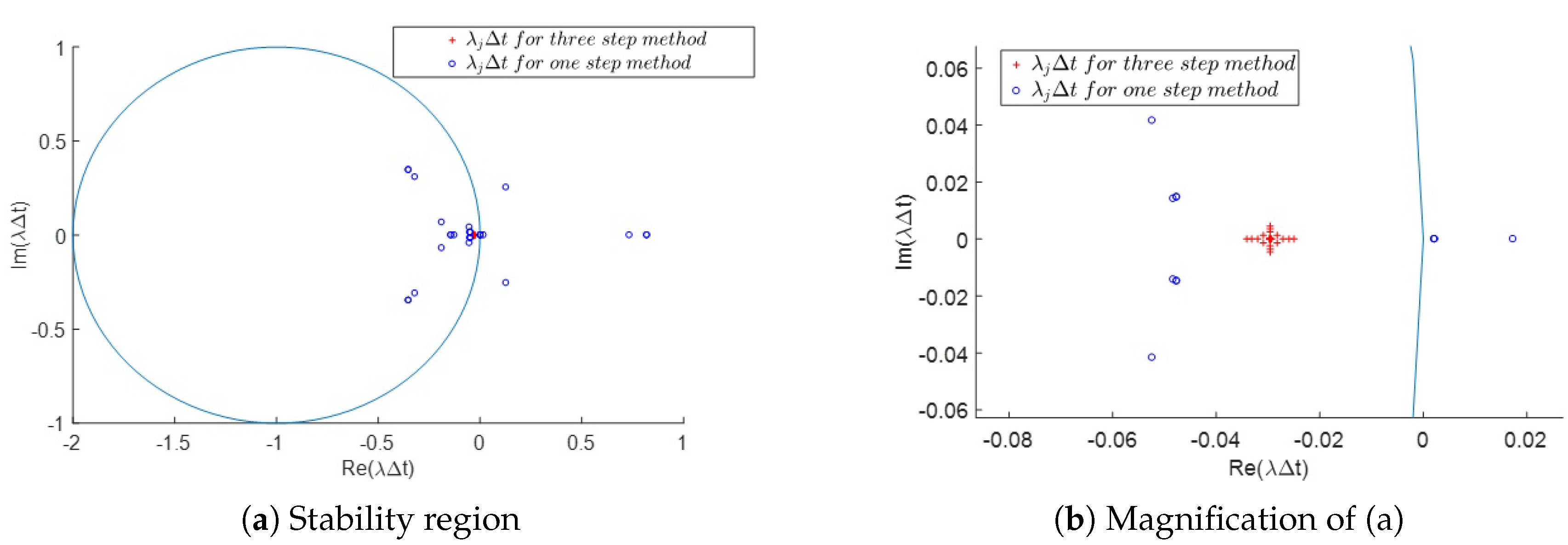
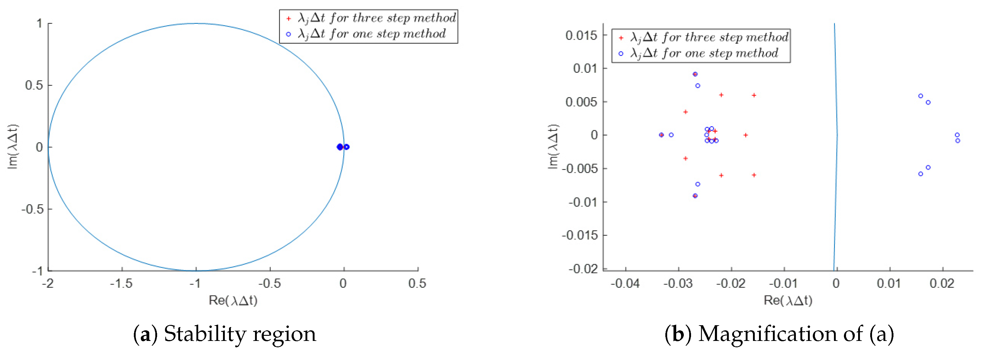
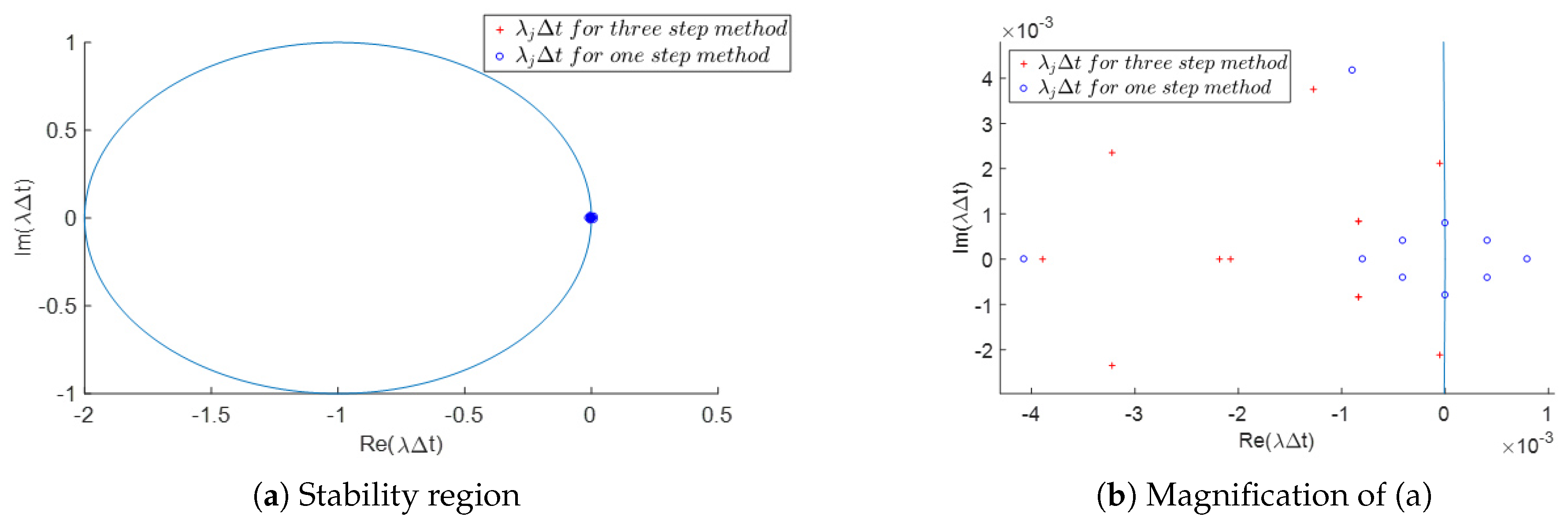
4. Stability Analysis
- 1.
- An absolutely stable method is one that generates a solution that tends to zero as tends to infinity,
- 2.
- A method is said to be A-stable, if it is absolutely stable for any possible choice of the time-step, , otherwise a method is called conditionally stable.
- 3.
- Absolutely stable methods keep the perturbation controlled,
- 4.
- The analysis of absolute stability for the linear model problem can be exploited to find stability conditions on the time step when considering some nonlinear problems.
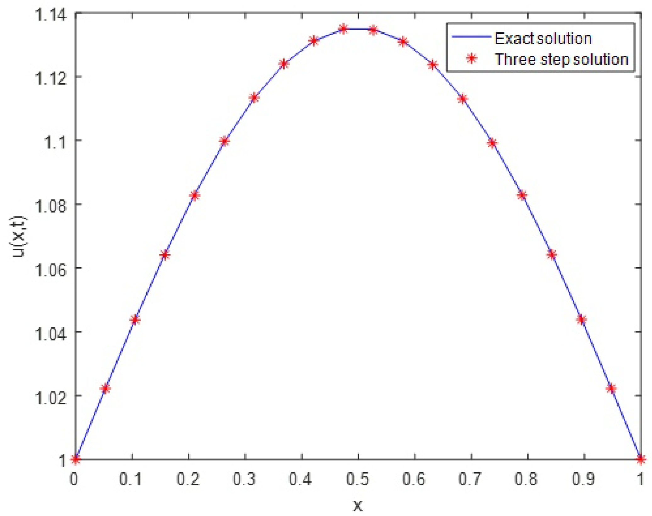
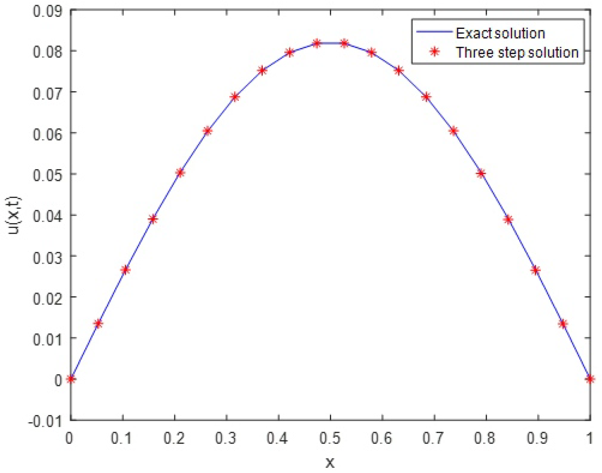
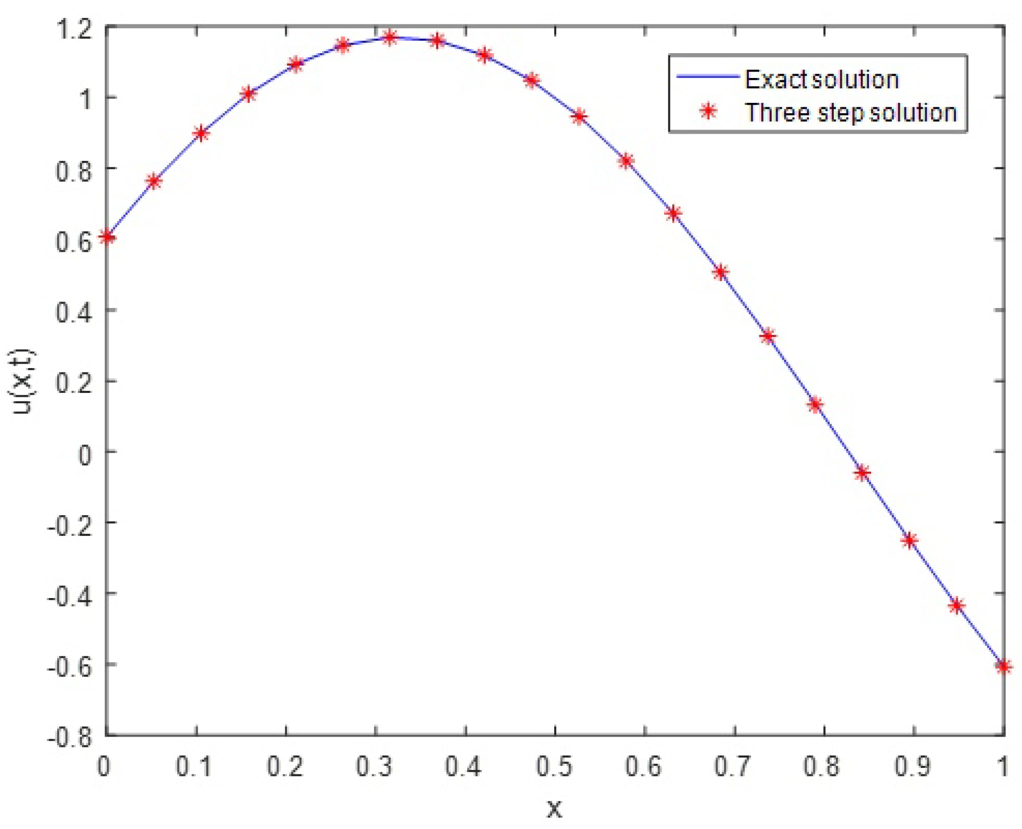
5. Numerical Examples
6. Conclusions
Author Contributions
Funding
Acknowledgments
Conflicts of Interest
References
- Nouria, K.; Siavashani, N.B. Application of Shannon wavelet for solving boundary value problems of fractional differential equations. Wavelet Linear Algebra 2014, 1, 33–42. [Google Scholar]
- Kumar, B.V.R.; Mehra, M. A three-step wavelet Galerkin method for parabolic and hyperbolic partial differential equations. Int. J. Comput. Math. 2006, 83, 143–157. [Google Scholar] [CrossRef]
- Iqbal, M.A.; Ali, A.; Din, S.T.M. Chebyshev wavelets method for heat equations. Int. J. Mod. Appl. Phys. 2014, 4, 21–30. [Google Scholar]
- Zhou, F.; Xu, X. Numerical solution of the convection diffusion equations by the second kind Chebyshev wavelets. Appl. Math. Comput. 2014, 247, 353–367. [Google Scholar] [CrossRef]
- Mohammadi, F.; Hosseini, M.M. A new Legendre wavelet operational matrix of derivative and its applications in solving the singular ordinary differential equations. J. Frankl. Inst. 2011, 348, 1787–1796. [Google Scholar] [CrossRef]
- Maleknejad, K.; Sohrabi, S. Numerical solution of Fredholm integral equations of the first kind by using Legendre wavelets. J. Appl. Math. Comput. 2007, 186, 836–843. [Google Scholar] [CrossRef]
- Sahu, P.K.; Ray, S.S. Legendre wavelets operational method for the numerical solutions of nonlinear Volterra integro-differential equations system. Appl. Math. Comput. 2015, 256, 715–723. [Google Scholar] [CrossRef]
- Chena, Y.M.; Weia, Y.Q.; Liub, D.Y.; Yu, H. Numerical solution for a class of nonlinear variable order fractional differential equations with Legendre wavelets. Appl. Math. Lett. 2015, 43, 83–88. [Google Scholar] [CrossRef]
- Heydari, M.H.; Maalek Ghaini, F.M.; Hooshmandasl, M.R. Legendre wavelets method for numerical solution of time-fractional heat equation. Wavelet Linear Algebra 2014, 1, 15–24. [Google Scholar]
- Islam, S.U.; Aziz, I.; Al-Fhaid, A.S.; Shah, A. A numerical assessment of parabolic partial differential equations using Haar and Legendre wavelets. Appl. Math. Model. 2013, 37, 9455–9481. [Google Scholar] [CrossRef]
- Yin, F.; Tian, T.; Song, J.; Zhu, M. Spectral methods using Legendre wavelets for nonlinear Klein\Sine-Gordon equations. J. Comput. Appl. Math. 2015, 275, 321–324. [Google Scholar] [CrossRef]
- Luo, W.H.; Huang, T.Z.; Gu, X.M.; Liu, Y. Barycentric rational collocation methods for a class of nonlinear parabolic partial differential equations. Appl. Math. Lett. 2017, 68, 13–19. [Google Scholar] [CrossRef]
- Luo, W.H.; Huang, T.Z.; Wu, G.C.; Gu, X.M. Quadratic spline collocation method for the time fractional subdiffusion equation. Appl. Math. Comput. 2016, 276, 252–265. [Google Scholar] [CrossRef]
- Jiang, C.B.; Kawahara, M. A three-step finite element method for unstesdy incompressible flows. Comput. Mech. 1993, 11, 355–370. [Google Scholar] [CrossRef]
- Kashiyama, K.; Ito, H.; Behr, M.; Tezduyar, T. Three-step explicit finite element computation of shallow water flows on a massively parallel. Int. J. Numer. Meth. Fluids 1995, 21, 885–900. [Google Scholar] [CrossRef]
- Quartapelle, L. Numerical Solution of the Incompressible Navier-Stokes Equations; Springer Basel AG: Basel, Switzerland, 1993. [Google Scholar]
- Kumar, B.V.R.; Sangwan, V.; Murthy, S.V.S.S.N.V.G.K.; Nigam, M. A numerical study of singularly perturbed generalized Burgers-Huxley equation using three-step Taylor-Galerkin method. Comput. Math. Appl. 2011, 62, 776–786. [Google Scholar] [CrossRef]
- Ford, W. Numerical Linear Algebra with Applications Using MATLAB; Elsevier: Waltham, MA, USA, 2015. [Google Scholar]
- Toledo, S. Locality of reference in LU decomposition with partial pivoting. SIAM J. Matrix. Anal. Appl. 1997, 18, 1065–1081. [Google Scholar] [CrossRef]
- Canuto, C.; Quarteroni, A.; Hussaini, M.Y.; Zang, T.A. Spectral Methods in Fluid Dynamics; Springer: Berlin, Germany, 1988. [Google Scholar]
- Quarteroni, A.; Saleri, F. Scientific Computing with MATLAB and Octave; Springer: Berlin/Heidelberg, Germany, 2006. [Google Scholar]
- Kumar, B.V.R.; Mehra, M. A wavelet-taylor galerkin method for parabolic and hyperbolic partial differential equations. Int. J. Comput. Meth. 2005, 2, 75–97. [Google Scholar] [CrossRef]
- Lambert, J.D. Numerical Methods For Ordinary Differential Systems; John Wiley & Sons Ltd.: Hoboken, NJ, USA, 1991. [Google Scholar]


| k | Method in [17] | One-Step Method | Three-Step Method | |
|---|---|---|---|---|
| 2 | 2.1847 | 1.8061 | ||
| 2 | unstable | unstable | ||
| 3 | ||||
| 3 | unstable | unstable |
| k | Method in [17] | One-Step Method | Three-Step Method | |
|---|---|---|---|---|
| 1 | ||||
| 1 | unstable | |||
| 2 | ||||
| 2 | unstable |
| k | Method in [17] | One-Step Method | Three-Step Method | |
|---|---|---|---|---|
| 1 | ||||
| 1 | unstable | |||
| 2 | ||||
| 2 | unstable |
| k | Method in [17] | One-Step Method | Three-Step Method | |
|---|---|---|---|---|
| 1 | ||||
| 1 | unstable | |||
| 2 | ||||
| 2 | unstable |
© 2018 by the authors. Licensee MDPI, Basel, Switzerland. This article is an open access article distributed under the terms and conditions of the Creative Commons Attribution (CC BY) license (http://creativecommons.org/licenses/by/4.0/).
Share and Cite
Torabi, M.; Hosseini, M.-M. A New Efficient Method for the Numerical Solution of Linear Time-Dependent Partial Differential Equations. Axioms 2018, 7, 70. https://doi.org/10.3390/axioms7040070
Torabi M, Hosseini M-M. A New Efficient Method for the Numerical Solution of Linear Time-Dependent Partial Differential Equations. Axioms. 2018; 7(4):70. https://doi.org/10.3390/axioms7040070
Chicago/Turabian StyleTorabi, Mina, and Mohammad-Mehdi Hosseini. 2018. "A New Efficient Method for the Numerical Solution of Linear Time-Dependent Partial Differential Equations" Axioms 7, no. 4: 70. https://doi.org/10.3390/axioms7040070
APA StyleTorabi, M., & Hosseini, M.-M. (2018). A New Efficient Method for the Numerical Solution of Linear Time-Dependent Partial Differential Equations. Axioms, 7(4), 70. https://doi.org/10.3390/axioms7040070