Article

Scalable and Fully Distributed Localization in Large-Scale Sensor Networks

1
The Center for Advanced Computer Studies, University of Louisiana, Lafayette, LA 70504, USA
2
Cisco Systems, Milpitas, CA 95035, USA
3
The Center for Cybersecurity, Old Dominion University, Norfolk, VA 23529, USA
4
Department of Computer Science, Stony Brook University, Stony Brook, NY 11790, USA
*
Author to whom correspondence should be addressed.
Axioms 2017, 6(2), 15; https://doi.org/10.3390/axioms6020015
Submission received: 30 March 2017 / Revised: 23 May 2017 / Accepted: 8 June 2017 / Published: 15 June 2017
(This article belongs to the Special Issue Discrete Geometry and its Applications)

Abstract

:
This work proposes a novel connectivity-based localization algorithm, well suitable for large-scale sensor networks with complex shapes and a non-uniform nodal distribution. In contrast to current state-of-the-art connectivity-based localization methods, the proposed algorithm is highly scalable with linear computation and communication costs with respect to the size of the network; and fully distributed where each node only needs the information of its neighbors without cumbersome partitioning and merging process. The algorithm is theoretically guaranteed and numerically stable. Moreover, the algorithm can be readily extended to the localization of networks with a one-hop transmission range distance measurement, and the propagation of the measurement error at one sensor node is limited within a small area of the network around the node. Extensive simulations and comparison with other methods under various representative network settings are carried out, showing the superior performance of the proposed algorithm.

1. Introduction

Geographic location information is imperative to a variety of applications in wireless sensor networks, ranging from position-aware sensing to distributed data storage and processing, geographic routing and nodal deployment. While global navigation satellite systems (such as GPS) have been widely employed for localization, integrating a GPS receiver in every sensor of an entire large-scale sensor network is unrealistic. Moreover, some application scenarios prohibit the reception of satellite signals by part or all of the sensors, rendering it impossible to solely rely on global navigation systems.
Even for those ranging information-based localization schemes, extra equipment installed to measure the distance or the angle between nodes can also lead to a dramatic increase of network cost. To this end, many interesting approaches have been proposed for localization with mere connectivity information. Each node only knows which nodes are nearby within its one-hop communication radio range, but does not know how far away and in what direction its neighbors are.

1.1. Challenges of Previous Approaches

Previous localization methods with mere connectivity have mainly focused on dimension reduction of multidimensional datasets based on the input distance matrix, which is approximated by hop counts between each possible pair of nodes. The two major methods, multi-dimensional scaling (MDS) based [1,2,3] and neural network based [4,5], achieve the highest localization accuracy and yield coordinates of sensor nodes that preserve the distance matrix between the data points of the input space and the output space (i.e., a 2D plane) as much as possible.
One of the major problems for MDS-based methods is their low scalability. The time complexity for obtaining the distance matrix is O ( n m ) where n and m are the number of vertices and edges, respectively. The time complexity to compute the two largest eigenvalues and the corresponding eigenvectors is O ( n 2 ) . With the increase of a network size n, the computational cost is prohibitive. Another issue is that they are inherently centralized. As a sensor network grows large in size, centralized computation has a fundamental bottleneck at nodes near the sink as each sensor node has a limited power and computation capability. Therefore, a distributed algorithm is highly preferred especially for a large-scale network. Different algorithms have been proposed to overcome these disadvantages. A basic approach is to partition the network into many subnetworks and compute the localization of each subnetwork, then merge these subnetworks together. This method requires delicate strategies and great caution in the merging stage.
For neural network-based methods, stability is their major problem due to the non-convex shape of their minimized energy. Although several approaches have been proposed to increase the possibility to escape from local minima of the minimized energy, the selection of initial values is still crucial for the final localization results [5].

1.2. Our Approach

We propose a novel localization algorithm that overcomes the major difficulties of conventional MDS and neural network-based methods. We first explain the basic idea using a smooth and planar surface and then transform it to sensor network localization.
Let us consider a smooth and planar surface. It is flat everywhere, so the Gaussian curvature, which measures how much a surface is curved and can be computed based on local distance information, equals zero at every point of the surface. Assume we only have approximated distance information instead of the exact one of the surface. Such approximated distance generates non-zero Gaussian curvatures, which induce a curved surface instead of a planar one. We can distort the approximated distance such that the deformed one generates zero Gaussian curvatures for every point, which guarantees that a surface can be embedded in plane. The tool we apply to distort the approximated distance is Ricci flow [6].
Given a large-scale sensor network deployed on a plane, we can extract a triangular mesh structure from the connectivity graph of the network such that the mesh structure approximates well the geographic structure of the sensor network. Specifically, we uniformly select a set of landmark nodes such that any two neighboring landmarks are a fixed Khops away. Landmarks initiate local flooding to build a landmark-based Voronoi diagram of the network such that any non-landmark node is within k hops of some landmark. We can build a triangulation based on the dual of the landmark-based Voronoi diagram. Each vertex of the triangulation is a landmark node. Each edge connecting two neighboring vertices is the shortest path between the two neighboring landmark nodes.
We can consider the triangular mesh as a discrete approximation of a smooth and planar surface. The local distance information of the mesh is discrete and represented by the approximated edge lengths (i.e., a fixed K-hop). The Gaussian curvature of the mesh is also discrete and can be computed based on the approximated edge lengths. Discrete Ricci flow deforms the length of each edge such that the deformed edge lengths induce zero Gaussian curvature at each vertex of the mesh. The deformed edge lengths guarantee that the triangular mesh can be embedded in the plane. We call such edge lengths a flat metric. However, there exists an infinite number of flat metrics. Each one of them can isometrically embed the triangular network into the plane. The key is which one of those flat metrics introduces the minimal deformation to the initially approximated edge length (i.e., achieves the minimal localization error). We prove that we can obtain an optimal flat metric with the least deformation from an initially non-flat one by controlling the condition of boundary vertices. The theorem is the foundation of our paper. Computing the optimal flat metric is the key step of our algorithms. Based on the computed optimal flat metric, localization (i.e., isometric embedding of the network to plane) is straightforward.
In our algorithm, all of the involved computations for each node only require information from nodes within its one-hop transmission range; therefore, it is fully distributed without cumbersome cutting and merging process. The proposed method is numerically stable, free of the choice of initial values and local minima with a theoretical guarantee. The computational cost and communication cost are both linear to the size of the network, so the method is scalable, suitable for large ad hoc networks with thousands of highly resource-constrained sensor nodes (processor, memory and power) that have a limited communication radio range.
Although accurate distance measurement is too expensive, or even impossible for a network with thousands or even millions of sensors, it is possible for a node to approximate its distance to nearby nodes within the one-hop transmission range in practice. If the range distance information is available, even with unavoidable measurement errors, our algorithm can incorporate the approximated one-hop distance information to further improve the localization accuracy. The impact of the measurement error at one node on the localization of other nodes of the network decreases dramatically in terms of the distance between them. This limited error propagation also contributes to the high scalability and localization accuracy of our proposed algorithms.
The rest of this paper is organized as follows. Section 2 gives a brief review of related works. Section 3 introduces the theoretical background of the proposed optimal flat metric-based localization algorithms. Section 4 describes the localization algorithm with mere connectivity information step by step. Section 5 discusses the localization algorithm with one-hop distance measurement. Section 6 presents the simulation results under various scenarios and different network topologies. Extensive comparisons of the proposed localization algorithm with previous methods are also conducted in Section 6. Section 7 concludes the paper and gives future directions.

2. Related Works

With mere connectivity information available, three major techniques are employed in current state-of-the-art localization schemes: multi-dimensional scaling (MDS), neural networks and graph embedding.
MDS is a non-linear dimension reduction and data projection technique that transforms the distance matrix into a geometric embedding (e.g., a planar embedding for 2D sensor network localization). MDS-based localization was originally proposed in [1]. It constructs a proximity matrix based on the shortest path distance (approximated by hop counts) between all pairs of nodes in the network. The singular value decomposition (SVD) is employed to produce the coordinates matrix that minimizes the least square distance error. Finally, it retains the first two (or three) largest eigenvalues and eigenvectors as 2D (or 3D) coordinates. Subsequent improvements on MDS are made by dividing the graph into patches to enable distributed calculation [2,3]. In addition, [7] proposes to apply SVD to the matrix based on a set of beacon nodes only and, thus, reduces complexity. A similar idea is adopted in [8], with the simplex method (instead of SVD) for error minimization.
The second method is based on neural networks [4,5], where non-linear mapping techniques and neural network models such as self-organizing map (SOM) are employed for dimension reduction of multidimensional datasets, yielding coordinates of sensor nodes that preserve the distances (also approximated by hop counts) between the data points of the input space and the output space (i.e., a 2D plane) as much as possible.
The localization algorithms based on rigid graph embedding theory [9,11,10] aim to create a well-spread and fold-free graph that resembles the given network. They focus on finding a globally rigid graph, which can be embedded without ambiguity in the plane. While with the mere globally rigid structure, like a topological disk triangulation in [9], there exist an infinite number of flat metrics that induce different planar embedding as long as the total Gaussian curvatures satisfy the discrete Gauss–Bonnet theorem as discussed in Section 3. A brute-force way is applied to find one planar embedding of the extracted global structure, which in general can not be easily guaranteed. Therefore, compared with MDS and neural network-based approaches, the graph rigidity-based methods exhibit lower localization accuracy in general.
A special graph embedding problem is unit disk graph embedding. Assuming the transmission model of a sensor network is unit disk graph (UDG) model with transmission range one, there exists an edge between two nodes in the connectivity graph of the network if and only if the Euclidean distance between the two nodes is no more than one. Embedding such a unit disk graph into the plane is NP-hard. Kuhn et al. in [12] proved a non-approximability result for the problem of embedding a given unit disk graph. Later, Moscibroda et al. in [13] introduced a polynomial algorithm to embed a unit disk graph into plane. The quality of the embedding, measured as the ratio of the maximum edge length to the minimum distance between two non-neighboring nodes, is O ( log 2.5 n log log n ) with n the size of the network. Note that the unit disk graph embedding achieves a different goal compared with the discussed localization algorithms. Given a network modeled by UDG, a unit disk graph embedding minimizes the violation of the unit disk constraints, but not necessarily the localization error that is in general measured as the ratio of the average node distance error and the average one-hop communication radio range.
Localization with noisy distance and angle information is discussed and distributed localization methods are proposed in [14]. If only distance measurement information is available, both the multi-dimensional scaling (MDS) and neural network-based methods are flexible to incorporate distance information to improve localization accuracy. Previous research assumes a given network has not only a small fraction of sensors with a priori coordinate knowledge, but also distance measurement between pairs of nodes with long distances. One representative work is the distributed weighted-multidimensional scaling (dwMDS) algorithm proposed to give more weight to range measurements that are believed to be more accurate and select neighbors adaptively [15]. Meanwhile, in this paper, we limit the discussion to localization based on distance measurement within the one-hop communication radio range to limit the communication cost of a large-scale sensor network.

3. Optimal Flat Metric

Before giving the details of the proposed optimal flat metric-based localization algorithms in Section 4 and Section 5, we introduce briefly the concepts of metric and Gaussian curvature in Section 3.1, which provide the necessary background knowledge of the algorithms. Specifically, we introduce discrete surface Ricci flow in Section 3.2, a tool we apply to compute the optimal flat metric that induces a planar localization of a given sensor network with a minimal localization error. We then discuss the condition to find the optimal flat metric and give the optimal flat metric theorem, which serves as the foundation of the proposed algorithms in Section 3.3. Table 1 summaries the symbols we use in the paper.

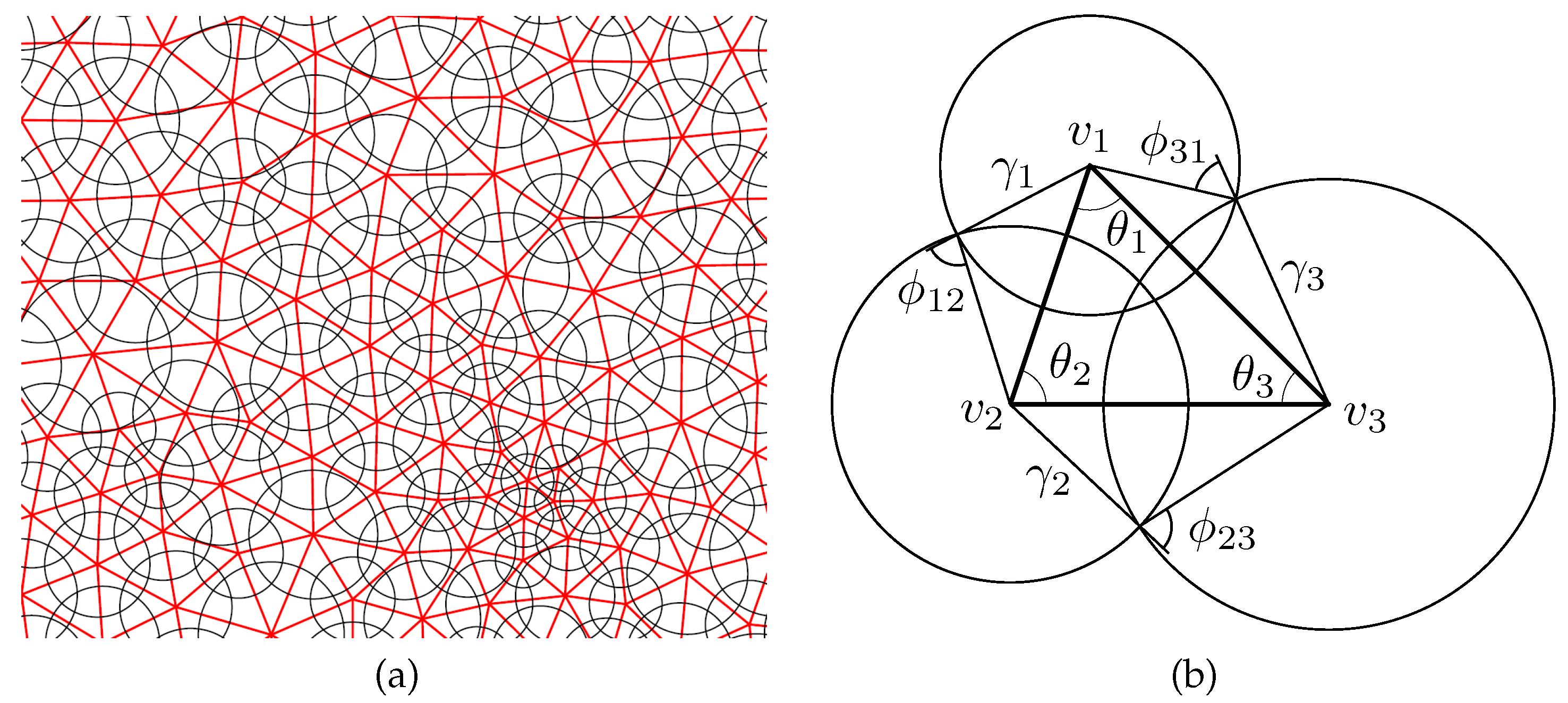
3.1. Discrete Metric and Gaussian Curvature

In the discrete setting, we denote M = ( V , E , F ) a triangulated surface (or mesh in short) embedded in R 3 , consisting of vertices (V), edges (E) and triangle faces (F). Specifically, we denote v i V a vertex with id i; e i j E an edge with two ending vertices v i and v j ; f i j k F a triangle face with vertices v i , v j and v k .
Definition 1 (Discrete metric).
A discrete metric on M is a function l : E R + on the set of edges, assigning to each edge e i j E a positive number l i j , such that all triangles satisfy the triangle inequalities f i j k F : l i j + l j k > l k i .
Edge lengths of M define a discrete metric. If M can be embedded in the Euclidean plane R 2 , we call its metric a flat metric.
Definition 2 (Discrete Gaussian curvature).
Denote θ i j k the corner angle attached to vertex v i in face f i j k and M the boundary of M; the discrete Gaussian curvature K i on v i V is defined as the angle deficit at v i :
K i = 2 π f i j k F θ i i j , v i M , π f i j k F θ i j k , v i M .
We can compute corner angles directly from edge lengths, so the discrete metric solely determines the discrete Gaussian curvature of M. If M can be embedded in the plane, it is intuitive and also obvious from Equation (1) that the flat metric induces zero Gaussian curvatures for all non-boundary vertices.
The well-known Gauss–Bonnet theorem says that the total Gaussian curvature of M is solely determined by its topology:
Theorem 1 (Discrete Gauss–Bonnet theorem).
Denote b the number of boundaries. Denote χ ( M ) the Euler characteristic number of M and χ ( M ) = 2 b . The total Gaussian curvature of M is a topological invariant. It holds as follows:
v i V K i = 2 π χ ( M ) .

3.2. Discrete Surface Ricci Flow

Ricci flow was first introduced by Richard Hamilton in his seminal work [6] in 1982. Suppose S is a smooth surface with a Riemannian metric g . The Ricci flow deforms the metric g ( t ) according to the Gaussian curvature K ( t ) (induced by itself), where t is the time parameter:
d g i j ( t ) d t = 2 K ( t ) g i j ( t ) .
If we replace the metric in Equation (3) with g ( t ) = e 2 u ( t ) g ( 0 ) , then the Ricci flow can be simplified as:
d u ( t ) d t = 2 K ( t ) ,
which states that the metric should change according to the curvature.
The Ricci flow can be easily modified to compute a metric with a user-defined curvature K ¯ as the following,
d u ( t ) d t = 2 ( K ¯ K ) .
With this modification, the solution metric g ( ) can be computed, which induces the curvature K ¯ .
Conformal metric deformation preserves infinitesimal circles and the intersection angles among them. Ricci flow defined in Equation (3) is proven in [16,17] to be convergent. The final metric is conformal to the original one. Moreover, at any time t, the metric g ( t ) is conformal to the original one g ( 0 ) .
Later, Chow and Luo [18] proved a general existence and convergence theorem for discrete Ricci flow on surfaces.
To briefly introduce the concept of discrete surface Ricci flow, we start from the concept of the circle packing metric given by Thurston in [19] as shown in Figure 1. We assign each v i a circle and denote γ i its radius. The radius function is Γ : V R + . The two circles at v i and v j of edge e i j intersect with an acute angle, denoted as ϕ i j and called the weight of e i j . The edge weight function is then Φ : E [ 0 , π 2 ] .
The length l i j of e i j can be computed from the circle radii of its two ending vertices γ i , γ j and its weight ϕ i j from the cosine law:
l i j 2 = γ i 2 + γ j 2 + 2 γ i γ j cos ϕ i j .
Definition 3 (Circle packing metric).
A circle packing metric of a mesh M includes the circle radius function and the edge weight function.
Given a discrete surface, we use circles with finite radii to approximate the infinitesimal circles; conformal deformation of a circle packing metric to approximate continuous metric deformation. Since two circle packing metrics ( Γ 1 , Φ 1 ) and ( Γ 2 , Φ 2 ) on the same mesh are conformally equivalent if Φ 1 Φ 2 , a conformal deformation of a circle packing metric only modifies the vertex radii and preserves the intersection angles on the edges.
Denote u i = log γ i , K ¯ i and K i the target and current Gaussian curvatures of v i , respectively, and t the time. The discrete Ricci flow is defined as follows:
d u i ( t ) d t = ( K ¯ i K i ( t ) ) .
Discrete Ricci flow continuously deforms the circle packing metric according to the difference between the current and target Gaussian curvatures in a heat-like diffusion process. Convergence of discrete surface Ricci flow is proven in [18]. The final circle packing metric induces the one that satisfies the target Gaussian curvatures.
Discrete Ricci flow can be formulated in a variational setting, namely it is a negative gradient flow of a special energy form. We define a mesh M with edge weight Φ a weighted mesh, denoted as ( M , Φ ) . We represent a circle packing metric on ( M , Φ ) by a vector u = ( u 1 , u 2 , , u n ) T and Gaussian curvatures at vertices by the curvature vector K = ( K 1 , K 2 , , K n ) T , where n is the number of vertices. For two arbitrary vertices v i and v j , the following symmetric relation holds:
K i u j = K j u i .
Let ω = i = 1 n K i d u i be a differential one-form [20]. The symmetric relation guarantees that the one-form is closed (curl free) in the metric space.
d ω = i , j ( K i u j K j u i ) d u i d u j = 0 .
By Stokes theorem, the following integration is path independent and called discrete Ricci energy.
f ( u ) = u 0 u i = 1 n ( K i ¯ K i ) d u i ,
where u 0 is an initial circle packing metric that induces the surface original metric. The discrete Ricci energy has been proven to be strictly convex in [18]. The global minimum uniquely exists, corresponding to the desired metric u ¯ that induces user-defined curvature k ¯ . The discrete Ricci flow is a negative gradient flow of the discrete Ricci energy, converging to the global minimum.
Furthermore, the speed of convergence can be estimated by the following formula [18]:
| K i ( t ) K ¯ i | < c 1 e c 2 t , c 1 , c 2 > 0 ,
where c 1 and c 2 are constant; namely, the convergence is exponentially fast.

3.3. Optimal Flat Metric

Analytically, the distortion of the metric at each vertex is given by u i . This motivates us to define the total distortion energy as:
E ( K ) = K 0 K ¯ i = 1 n u i d K i ,
where K ¯ and K 0 represent the set of target and initial vertex Gaussian curvatures, respectively. The integration is along an arbitrary path from K 0 to the target curvature K ¯ . This energy is the Legendre dual to the Ricci energy given in Equation (8). Therefore, it is also convex, and it has a unique global minimum for a given K ¯ .
All of the possible u ’s form the admissible metric space, and all of the possible K ’s form the admissible curvature space. According to the Gauss–Bonnet theory (Equation (2)), the total Gaussian curvatures of M must be 2 π χ ( M ) . A curvature vector K is admissible if there exists a metric vector u on M, which induces K .
Define:
Ω = { K i = 1 n K i = 2 π χ ( M ) and K i = 0 v i M }
the set of K ’s such that the sum of Gaussian curvatures of vertices satisfies the Gauss–Bonnet theorem, and the Gaussian curvature of all interior vertices is zero. Ω induces the set of all possible flat metrics of M.
We formulate our problem as:
min K Ω E ( K ) .
Among all possible flat metrics of M induced from the set of K ’s, we want to find the one introducing the least distortion from the initially estimated curved metric of M.
Theorem 2 (Optimal flat metric theorem).
The solution to the optimization problem (9) is unique and satisfies:
u j = c o n s t , v j M .
Proof. 
The distortion energy E ( K ) is convex. The domain Ω is a linear subspace of the original domain { K | i K i = 2 π χ ( M ) } . Therefore, the restriction of E ( K ) on Ω is still convex; it has a unique global optimum at an interior point. The gradient of the energy is E ( K ) = ( u 1 , u 2 , , u n ) . At the optimal point, the gradient is orthogonal to Ω . Assume v i M , 1 i m , then the normal vector to Ω is given by ( 1 , 1 , 1 , 0 , , 0 ) . Therefore, the gradient is along the normal vector. Therefore, Equation (10) holds. ☐
We set the constant in Equation (10) as one. We also set the following two conditions for the target metric of discrete Ricci flow: set the target Gaussian curvatures of all interior vertices to zero so that the final metric is a flat one; deform only the metrics of interior vertices during the process of deforming the estimated metric so that the final flat metric is an optimal flat one. We apply discrete Ricci flow to find the target metric. Since discrete Ricci flow is proven in [18] as a negative gradient flow of a convex shape energy, it is guaranteed to find the optimal flat metric regardless of the step length or initial values.

4. Localization with Mere Connectivity

We explain the proposed localization algorithm with mere network connectivity in this section. Specifically, the input of the algorithm is a connectivity graph of a network. Vertices represent the sensor nodes. Edges represent the communication links. Each sensor node knows a set of neighboring nodes within its one-hop communication range without the knowledge of distance or angle. The output of the algorithm is a set of planar coordinates of the whole of the network nodes that may differ in the set of GPS positions of the network a scaling, translation and rotation. We first extract a triangular mesh from the connectivity graph and then apply discrete surface Ricci flow to compute an optimal flat metric as introduced in Section 4.1. We then isometrically embed the network into 2D plane based on the computed flat metric in Section 4.2. We analyze the time complexity and communication cost of the algorithm in Section 4.3 and provide discussions in Section 4.4.

4.1. Computing Optimal Flat Metric with Mere Connectivity

Given a large-scale sensor network with mere connectivity, we apply a simple distributed scheme as discussed in [22,23,21] to uniformly select a set of landmark nodes. Any two neighboring landmarks are a fixed k hops away ( k = 4 in our tests) in the connectivity graph of the network. Landmarks initiate local flooding to build a landmark-based Voronoi diagram of the network such that any non-landmark node is within k hops of some landmark. The adjacency of these Voronoi cells gives rise to a dual combinatorial Delaunay complex (CDC). CDC is not necessarily planar because there may exist some crossing edges. We then apply the method introduced in [23] to remove crossing edges from the CDC. Vertices of the resulting planar graph are the set of landmarks. An edge connecting two neighboring vertices is the shortest path between the two landmarks in the network. A face of the planar graph is an n-polygon with n 3 . We can simply consider all n-polygons with n > 3 as inner holes of the network. In practice, we add one virtual edge (i.e., a shortest path) connecting a pair of non-neighboring vertices of a four-polygon. A four-polygon is then split into two triangles.
A landmark node-based graph may have dangling vertices or edges as shown in Figure 2. A dangling vertex is a vertex belonging to more than one boundary. We remove dangling vertices by vertex split operation. As shown in Figure 2a, v 1 is connected with boundary vertices v 2 , v 4 , v 5 and v 7 that belong to two disconnected boundaries with boundary edges marked with red color. We find a sensor node closest to v 1 and mark it as a landmark node, as well. Denote the newly-added landmark as v 1 . v 1 is connected with v 5 and v 7 , and v 1 is connected with v 2 and v 4 . The previously disconnected boundaries are merged into one. Similarly, a dangling edge is an edge belonging to more than one boundary. We remove dangling edges by the edge removal operation. As shown in Figure 2b, e 01 belongs to two disconnected boundaries. We remove this edge such that the previously disconnected boundaries are merged into one. The graph now is a triangular mesh with each face a triangle, a boundary vertex or edge belonging to exactly one boundary.
Denote the constructed triangular mesh M; we assume each edge of M with unit edge length. We then construct an initial circle packing metric ( Γ 0 , Φ ) of M. We assign each vertex v i a circle with initial circle radius γ i = 1 , so initially, u i = log γ i = 0 . The intersection angle of the two unit circles at v i and v j is the edge weight of e i j . Since a boundary edge of M is adjacent with only one triangle face, we can easily detect them and then mark their vertices. For those non-marked vertices (i.e., non-boundary vertices), we set their target Gaussian curvatures K ¯ to zero.
In each iteration of discrete Ricci flow, only non-marked vertices are involved. Specifically, each non-marked v i collects the u values from its direct neighbors and updates its adjacent edge length with l i j = e ( u i + u j ) . For each triangle f i j k adjacent with v i , v i can easily compute the corner angle θ i j k based on the inverse cos law:
θ i j k = cos 1 l k i 2 + l i j 2 l j k 2 2 l k i 2 l i j 2 .
Then, v i computes its current discrete Gaussian curvature K i as the excess of the total angle sum at v i as Equation (1). If for every non-marked v i , the difference between its target Gaussian curvature K ¯ i that is set to zero and current Gaussian curvature K i is less than a threshold (we set it to 1 × 10 5 in our tests), the discrete Ricci flow converges. Otherwise, each non-marked v i updates its u i : u i = u i + δ ( K ¯ i K i ) , where δ is the step length (we set it to 0.1 in our tests).
When the algorithm stops, all of the interior vertices have zero Gaussian curvature, which induces a flat metric of M. Since in each step of the algorithm, there is always no deformation of circle radii for boundary vertices (e.g., u i u i 0 = 0 , v i M ), according to Theorem 1, the computed flat metric introduces the least distortion to the initially estimated metric.

4.2. Isometric Embedding

Isometric embedding is a propagation process, starting from one vertex, embedding the whole triangular mesh into plane with the computed optimal flat metric (i.e., edge length) preserved. For simplicity, we let the vertex with the smallest ID (denoted as v 1 ) initiate the embedding process. Its planar coordinates are set to ( 0 , 0 ) , denoted as u v ( v 1 ) . Then, it arbitrarily selects one of its direct neighbors, e.g., v j , and sets the coordinates of v j to ( 0 , l i j ) . For vertex v k , adjacent to both v i and v j , it calculates the intersection points of the two circles with centers at v i and v j and the radii of l i k and l j k , respectively. Then, v j chooses one of the intersection points that satisfies ( u v ( v j ) u v ( v i ) ) × ( u v ( v k ) u v ( v i ) ) > 0 as the coordinates of v k . The procedure continues until all vertices of M have their planar coordinates.
If a triangular network has multiple boundaries (e.g., inner holes), we need to slice holes open to change the topology of the triangular network to a disk before embedding. For each boundary, an initiator with the smallest ID is elected. Since a boundary forms a closed loop, a boundary node always has exactly two boundary neighbors. The initiator will send out a message to a randomly chosen one of its boundary neighbors. The message contains a counter recording the size of the boundary that is initialized to one. When the neighbor receives the message, it will increase the counter by one and then forward the message to its boundary neighbor that is not the sender of the message. Eventually, the message will come back to the initiator. The initiator will then advertise the size of the boundary via a simple flooding on the triangular network. As a result, each initiator learns the sizes of boundaries of the network. Denote B i a boundary and B 0 the longest one. For each B i ( i > 0 ), through a local flooding, its initiator finds a shortest path L i to B 0 . Then, holes are “sliced” open along the set of shortest paths ( L 1 , L 2 , . . . ) , where each vertex on L i is split into two virtual vertices with one on each side. Such spliced vertex will have two sets of coordinates after embedding, and it will use the average as its planar coordinates.
For planar embedding of non-landmark nodes, each node n i finds its three nearest landmarks, denoted as v 1 , v 2 , v 3 with planar coordinates ( x 1 , y 1 ) , ( x 2 , y 2 ) and ( x 3 , y 3 ) , respectively. Let d 1 , d 2 and d 3 be the shortest distances (hop counts) of n i to v 1 , v 2 , v 3 , respectively. Then, n i computes its planar coordinates ( x i , y i ) simply by minimizing the mean square error among the distances:
j = 1 3 ( ( x i x j ) 2 + ( y i y j ) 2 d j ) 2 .
It is worth noting that the step of the isometric embedding of the proposed approach is fundamentally different from graph rigidity-based localization methods [9]. For an extracted global planar structure, our algorithm computes first the optimal flat metric with discrete Gaussian curvature equal to zero for all interior vertices, which guarantees that the embedding process can be determined at each step for every single edge; while in [9], the extracted structure is embedded into plane by minimizing a least square energy which cannot guarantee a global planar embedding, and the embedded network can still curve around and self-intersect.

4.3. Time Complexity and Communication Cost

The algorithm of extracting a triangular structure M from a network is completely local, so both its time complexity and communication cost are linear to the size of the network, denoted as n (the number of sensor nodes).
We then apply discrete Ricci flow to compute the optimal flat metric of M. The time complexity (the number of iterations) of discrete Ricci flow is given by C l o g ϵ δ , where C is a constant, ϵ is a threshold of curvature error and δ is the step length of each iteration [18]. Denote m the size of M. Since each vertex only needs to exchange u values with its direct neighbors, the communication cost is given by O ( C l o g ϵ δ g m ) , where g is the average vertex degree of M. Note that m < < n for a general network, and g is six for a triangular mesh.
During the isometric embedding step, two rounds of flooding are involved in slice holes of M open with communication cost O ( m ) . The embedding of M is a propagation process, with both the time complexity and communication cost O ( m ) .

4.4. Discussions

As indicated in [23], a large k to select landmarks decreases the number of crossing edges of a CDC. In practice, we prefer a small k such that the extracted planar graph can resemble the geometry of the underlying domain of a network better. In our simulations, k = 4 introduces only very few crossing edges on the CDCs of the testing networks. For the resulting non-triangular face of a planar graph with the removal of the detected crossing edges, we add virtual edges (i.e., shortest paths) connecting the pair of non-neighboring vertices of a non-triangular face to split it into triangle faces.
We apply the method introduced in [23] to remove crossing edges of a CDC. The method is proven to produce a planar graph if the transmission model of a given network is either the unit disk graph (UDG) or the quasi-unit disk graph (Quasi-UDG). In Section 6.2, we apply the same network to evaluate the performance of the proposed localization method with mere connectivity under different transmission models including the UDG model, Quasi-UDG model, log-norm model and the probability model. We assume sensor nodes of the network have identical transmission ranges. Legal triangular meshes can still be generated for the network with different transmission models, although the localization accuracy is lower for the network with the log-norm model or probability model.

5. Localization with Distance Measurement

It is possible for some networks to estimate the Euclidean distance between adjacent sensor nodes that are within the one-hop transmission range of each other. Two basic approaches are received signal strength (RSS) and time-differential-of-arrival (TDoA). RSS measures the power of the signal at the receiver and calculates the distance according to the propagation loss model. TDoA measures the differential propagation time of the received signal to determine the distance. Multiple measurements can be averaged to obtain more accurate results. RSS is easier to implement, while TDoA may achieve higher accuracy, but in general, measurement error is unavoidable. In our previous experiments [24], we let each sensor periodically broadcast a beacon message containing its node ID to its neighbors in a sensor network formed with crossbow motes. Based on received beacon messages, a node builds a neighbor list with the RSSI (received signal strength indicator) of corresponding links. The node applies RSSI to estimate the length of links by looking up an RSSI-distance table established by experimental training data. Our preliminary tests show that, under low transmission power, such estimation has an error rate around 20 % .
When distance information is available, we extend the proposed localization algorithm to incorporate it to achieve higher localization accuracy than with mere network connectivity. We give the implementation details of the algorithm in Section 5.1 and Section 5.2. We then discuss the time complexity and communication cost of the algorithm in Section 5.3. In Section 5.4, we show how distance measurement error at a single node of a network affects the localization performance of the whole network.

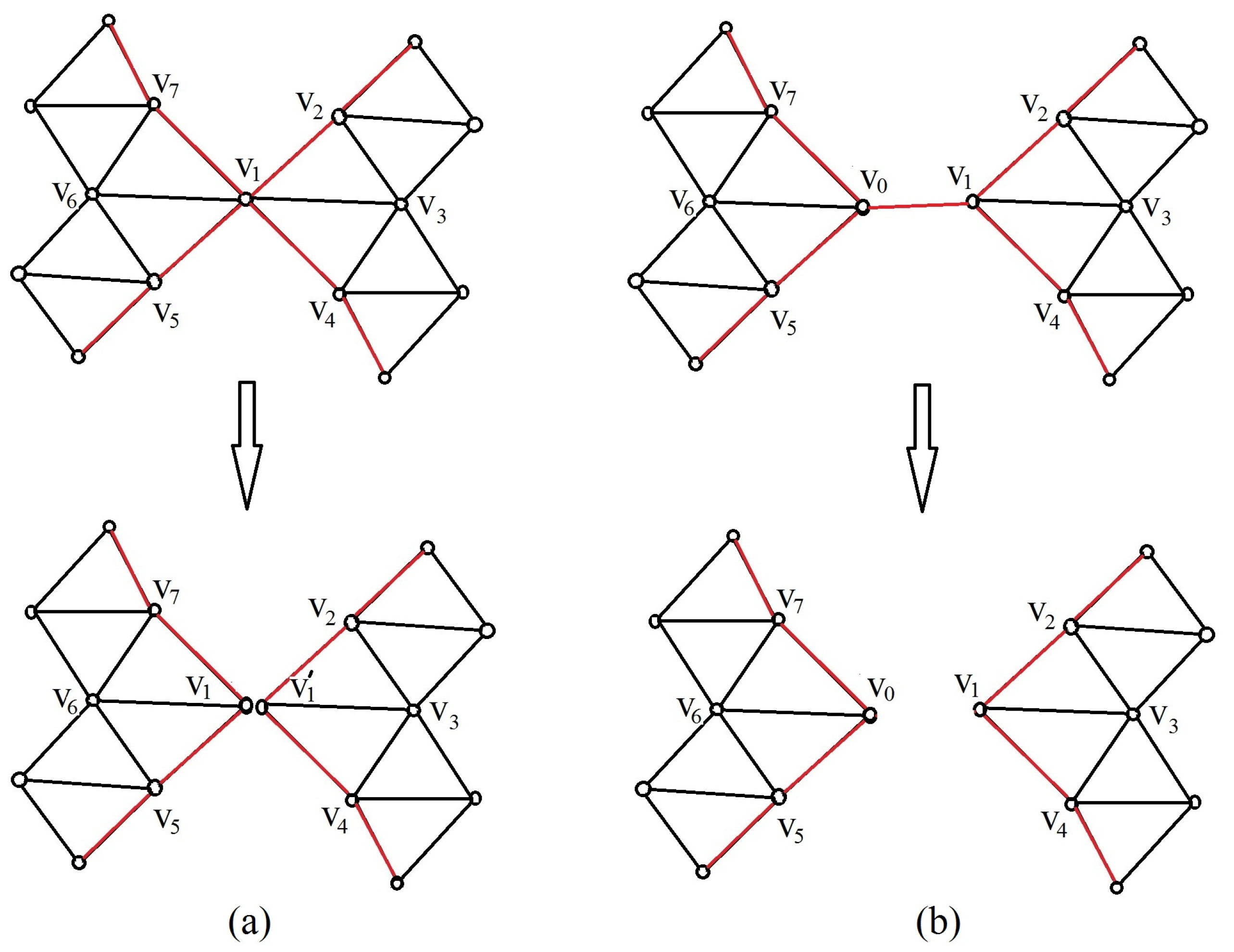
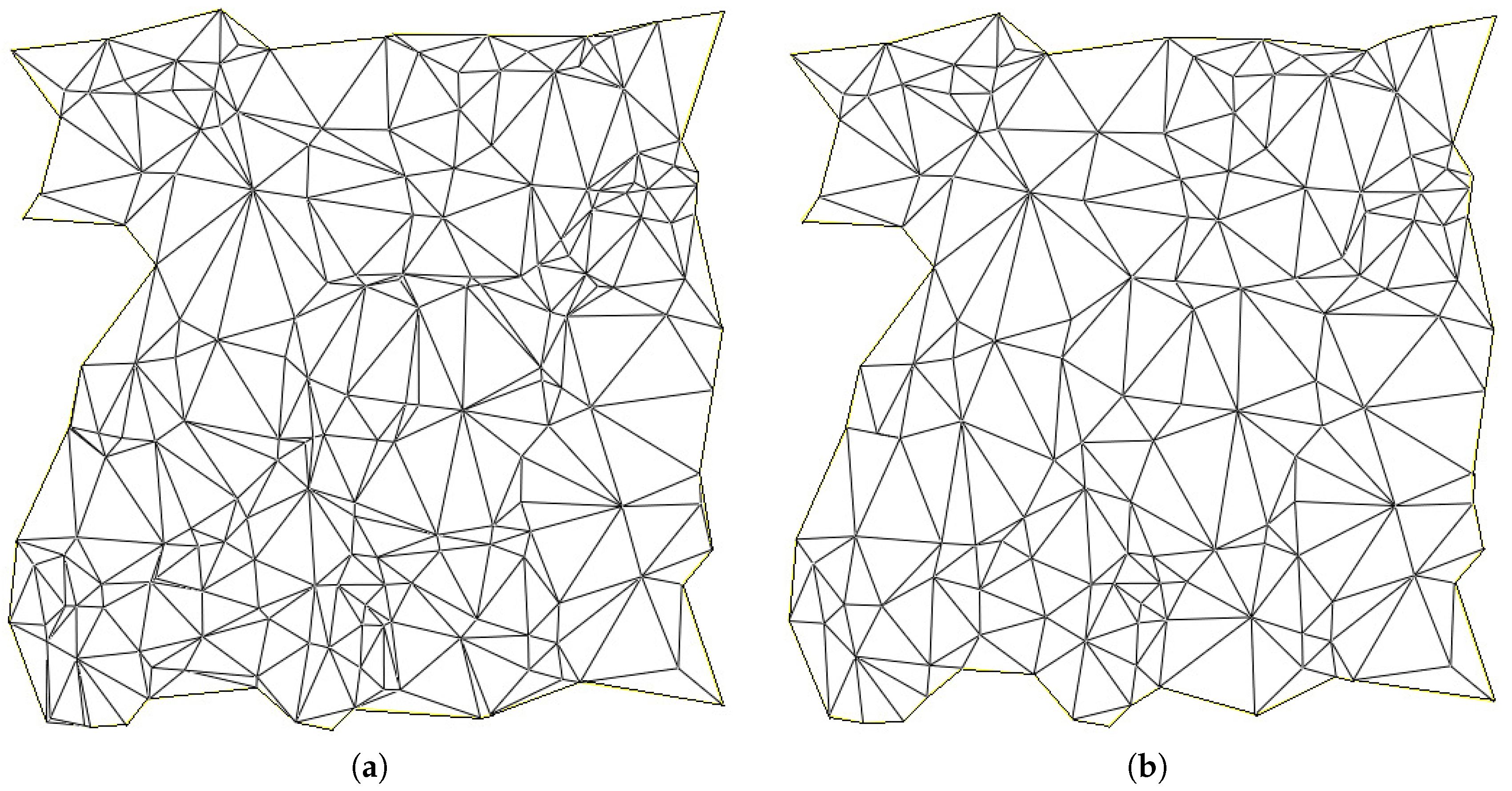
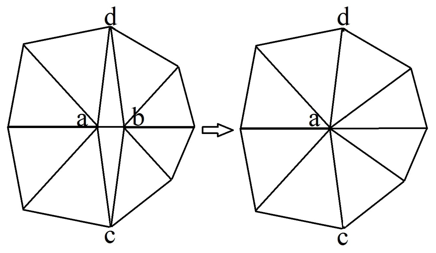
5.1. Constructing Triangulation

Given a sensor network with distance measurement within one-hop transmission range, we apply our previously-proposed algorithm [25] to generate a refined triangular mesh M such that vertices of M are the set of sensor nodes. An edge between two neighboring vertices indicates the communication link between the two sensors, and the edge length is the measured distance. The triangulation algorithm is distributed with no constraints on the communication model.
However, such a triangular mesh may have unavoidable skinny triangles especially when the node distribution is non-uniform. Note that a triangular mesh constructed based on mere network connectivity has all equilateral triangles because we assume a unit edge length for each edge, and the assumption is independent of the node density and distribution. As discussed in our previous work [26], solving discrete surface Ricci flow can be considered as solving a linear equation of the discrete Laplace–Beltrami operator defined on a triangular mesh. Skinny triangles increase the condition number of the linear equation, so a triangular mesh M with many skinny triangles may affect the numerical stability and the convergence speed of surface Ricci flow. Therefore, we need the following post-processing on a constructed triangular mesh with skinny triangles.
For each f i j k , we compute a ratio between the longest and shortest edge lengths of f i j k and denote it as r f i j k . Triangles with extremely high r f represent those skinny ones. To remove them, we define one operation, called short edge collapse, as illustrated in Figure 3. f a b c and f a b d have very high r f values. Both share the short edge e a b . The short edge collapse operation combines the two vertices v a and v b into one of them and removes faces f a b c and f a b d . In practice, we choose the vertex that results in smaller r f values than the other one after short edge collapse. As in the example shown in Figure 3, v a is chosen as the combined vertex. If the operation of one short edge collapse generates a larger r f than previous ones, we will not collapse the edge.
We first set a threshold of r f . The algorithm computes the r f value for each triangle and then sorts these r f values and puts them into a queue. Each time, the algorithm picks one triangle with currently the highest r f value and applies the short edge collapse operation. The algorithm stops when the highest r f value is below the threshold. Figure 4 gives one example. A triangular mesh constructed from a network with an extremely non-uniform node distribution has a maximal r f value close to 27, as shown in Figure 4a. After a series of short edge collapse operations, its maximal r f value is below four, as shown in Figure 4b.

5.2. Computing the Optimal Flat Metric with Distance Measurement

We construct an initial circle packing metric ( Γ 0 , Φ ) of M from provided distance measurements with the following procedures:
  • For each corner θ i j k attached to vertex v i in face f i j k , we compute a corner radius γ i j k for v i with respect to f i j k :
    γ i j k = l k i + l i j l j k 2 ,
    where l i j , l j k , l k i represent the distance measurements of edges e i j , e j k , e k i , respectively.
  • For each v i , we compute its initial circle radius γ i by averaging its attached corner radii computed from the previous step:
    γ i = 1 m f i j k F γ i j k ,
    where m is the number of the adjacent faces to v i (i.e., the vertex degree of v i ).
  • For each edge e i j , we compute its edge weight ϕ i j (the intersection angle of the two circles centered at v i and v j ) based on the Euclidean cosine law:
    cos ϕ i j = γ i 2 + γ j 2 l i j 2 2 γ i γ j .
With the constructed initial circle packing metric ( Γ 0 , Φ ) , we apply the algorithm introduced in Section 4.1 to compute the optimal flat metric and then the isometric embedding algorithm introduced in Section 4.2 to embed the given network into a plane.

5.3. Time Complexity and Communication Cost

To incorporate distance information into the localization algorithm introduced in Section 4, we need to incur some extra costs.
The method to initialize the circle packing metric is local. The time complexity and communication cost are both linear to the size of the network n, the number of sensor nodes.
The algorithm to extract a triangulation from the network connectivity graph based on distance measurement is also local and fully distributed. Both the time complexity and communication cost are linear to n [25].
The time complexity and communication cost of post-processing a triangulation are bounded by the number of edges of the triangular mesh. Denote v n the number of vertices, e n the number of edges and f n the number of triangle faces of a triangular mesh M; the well-known Euler–Poincaré theorem relates v n , e n and f n [27].
Theorem 3 (Euler-Poincaré Theorem).
Denote b the number of boundaries of a triangular mesh M. The following equation holds assuming M with zero number of handles:
v n e n + f n = 2 b .
Based on the Euler–Poincaré theorem, the following theorem shows that e n 3 v n .
Theorem 4.
Denote b the number of boundaries of a triangular mesh M, v n the number of vertices and e n the number of edges. The following equation holds:
e n = 3 v n + ( 3 b 6 ) .
Proof. 
Denote f n the number of triangle faces of M, e M the number of non-boundary edges and e M the number of boundary edges. Considering the two facts that each non-boundary edge is shared by two triangle faces and each triangle face has three edges, the following equation holds:
2 e M + e M = 3 f n ,
which gives:
f n = 2 3 e n ,
by ignoring boundary edges if:
e M < < e M .
According to Euler–Poincaré Theorem 12, the following equation also holds:
v n e n + f n = 2 b .
Plug Equation (14) into (15); we have:
v n e n + 2 3 e n = 2 b .
Then, we have:
e n = 3 v n + ( 3 b 6 ) .
Therefore, the time complexity and communication cost of post-processing a triangulation are O ( n ) .

5.4. Error Propagation

If the distance measurement error is introduced only by one single node, we show that the error propagation of the proposed localization algorithms decreases with the distance to the node.
According to the discrete Ricci curvature theory, the differential discrete curvature d K and discrete scaling factor d u satisfy the discrete Poisson equation:
d K = Δ d u ,
where Δ is the discrete Laplace–Beltrami operator.
Specifically, suppose v i is an interior vertex and v j is one of its neighboring vertices. f i j k and f j i l are the two faces adjacent to e i j . The power circle of f i j k is defined as a circle orthogonal to all three circles centered at v i , v j and v k with radii γ i , γ j and γ k respectively. Similarly, one can define the power circle of f j i l . Denote d i j the distance between the two power circles, l i j the length of e i j . For each e i j , we define a weight:
w i j = d i j l i j .
Then, we have:
d K i = j = 1 g w i j ( d u j d u i ) ,
where g is the vertex degree of v i .
Suppose a small perturbation of the curvature happens at v i , modeled as δ ( v v i ) . Such a perturbation is due to the measurement error of neighboring distances around v i . Then, the influence of the perturbation to the entire network can be estimated by Green’s function, G ( v , v i ) , such that Δ G ( v , v i ) = δ ( v v i ) . Roughly speaking, Green’s function on the plane is 1 2 π log 1 | v v i | . Therefore, the influence of the perturbation at one node is sublinear to others. The influence of the wrong measurements at one node on others decreases proportionally with their distances.

6. Simulations and Comparison

We carry out extensive simulations under various scenarios to evaluate the performance of our algorithm on networks with different topologies and how the performance is affected by different factors such as node density, the communication model (UDG, quasi-UDG, log-norm model and probability model) and a non-uniform node distribution. We compare our algorithm with those state-of-the-art localization methods, including the centralized MDS approach (MDS-MAP) [1], the distributed MDS approach (MDS-MAP(P)) [2], the centralized (C-CCA) neural network, and the distributed (D-CCA) neural network approaches [5].
We apply the proposed optimal flat metric-based method to localize the landmark nodes (points marked with red in Figure 5, Figure 6, Figure 7 and Figure 8). Those non-landmark nodes (points marked with grey in Figure 5, Figure 6, Figure 7 and Figure 8) in the network find their three nearest landmarks and compute their own coordinates. We then compute the difference of each node-pair’s distances in the original and localized networks. We calculate the localization error as the ratio of the average difference of node-pair distances and the one-hop communication radio range.

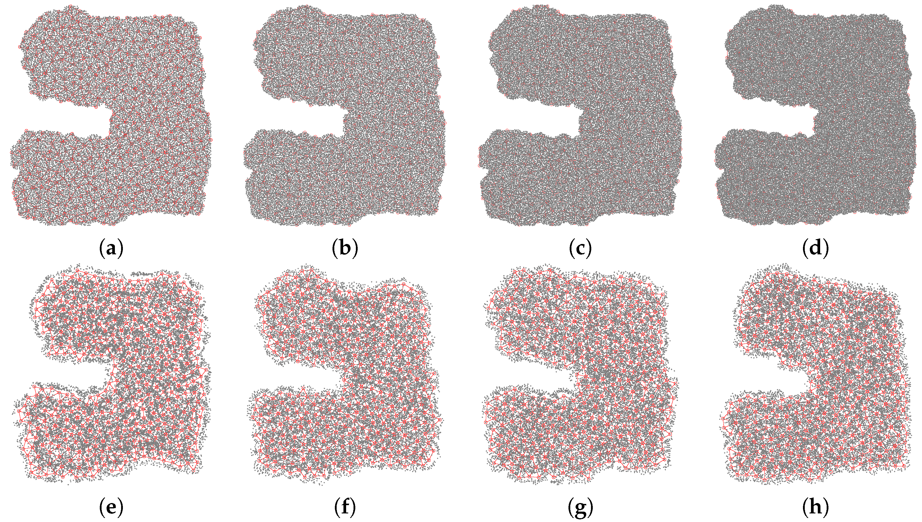
6.1. Networks with Variant Nodal Densities

In general, connectivity-based localization methods favor high nodal density, because hop counts approximate well the true shortest distance. Figure 5a–d gives a series of reversed C-shaped networks with mere connectivity information. All of the networks have the same communication radio range and are under the same transmission model, but the average nodal degree increases from 9–18. Figure 5e–h shows the localization results correspondingly. The localization error decreases from 0.514 0.246 . The trend is clear that the localization error decreases with the increase of nodal density.

6.2. Networks with Different Transmission Models

We still apply the same reversed C-shaped network to evaluate the performance of the proposed localization algorithm with mere connectivity under different transmission models, with average nodal degree d = 16.5 (under the UDG model). For a network with an identical communication radio range of sensor nodes, different transmission models induce different sets of landmarks because each node has different neighborhoods. We generate different triangular meshes accordingly. In our simulations, the transmission range of a UDG model is one. Two nodes are definitely connected when their distance is less than one. Under the Quasi-UDG model, two nodes are definitely connected when their distance is less than α = 0.75 , definitely not connected when their distance is larger than 1, while they have a probability of ρ = 0.5 to be connected when the distance is between α and one. Under the log-norm model [28], since the receiving power is log-normally distributed, we simplify it as: when the distance between two nodes is larger than one, they are not connected; when the distance is less than one, they have a probability P ( d ) to be connected, where d is the distance, and P ( d ) satisfies the log-normal distribution with α = 2 and σ = 4 . Under the probability model, when the distance of two nodes is less then one, they have a probability equal to a constant set to 0.65 to be connected. Figure 6 shows the localization results of the reversed C-shaped network with mere connectivity under different transmission models.
Among all of the transmission models, UDG model achieves the smallest localization error.

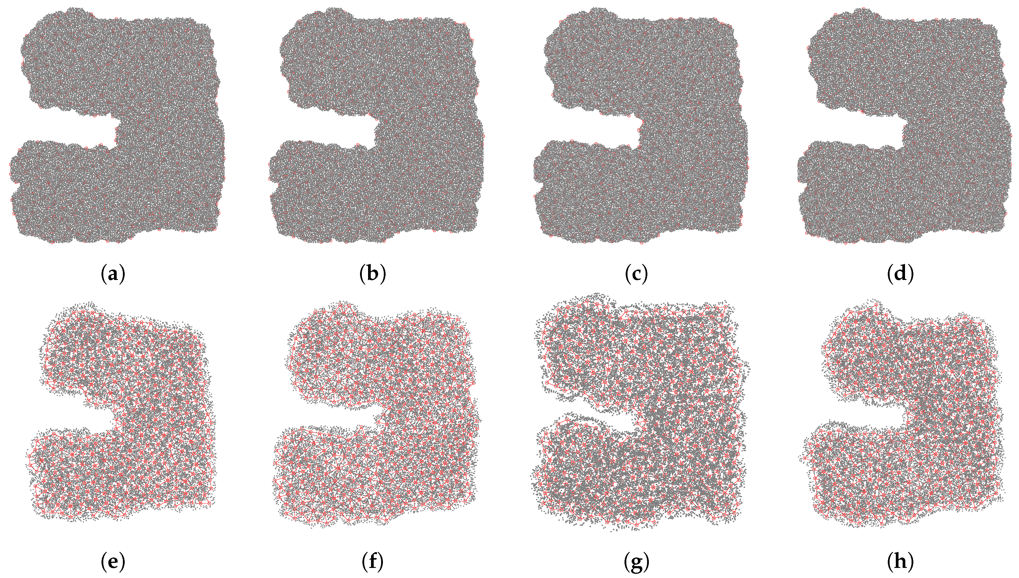
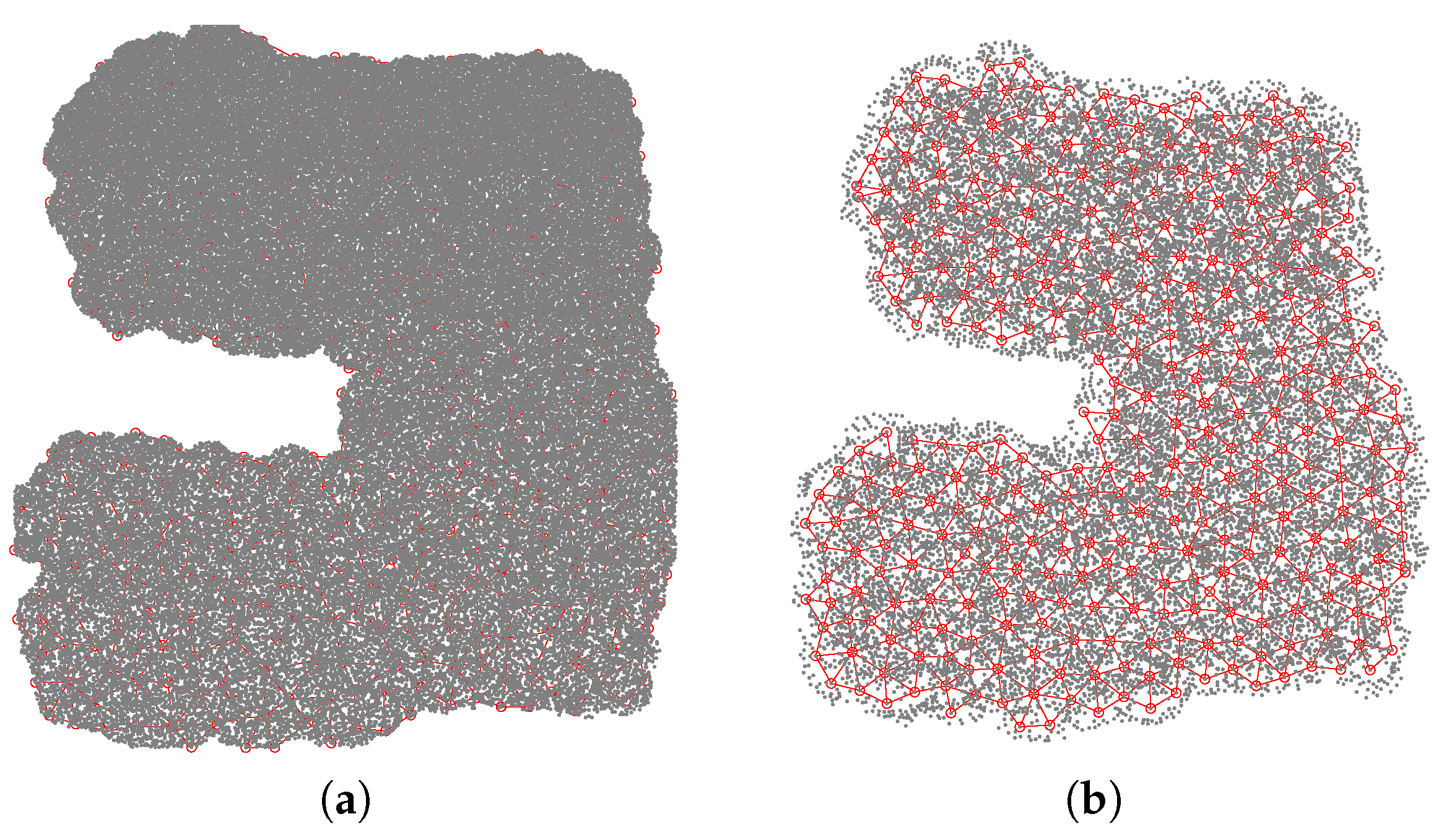
6.3. Networks with Non-Uniform Nodal Distribution

We also test the proposed optimal flat metric-based method with mere connectivity on a network with a non-uniform node distribution. The nodal density of the reversed C-shaped network shown in Figure 7a increases from the bottom to the top. Specifically, the nodal degree increases from 11.3 18.7 . Figure 7b shows the localization result with a slightly higher localization error 0.46 . The proposed algorithm can tolerate networks with a moderately non-uniform nodal distribution.

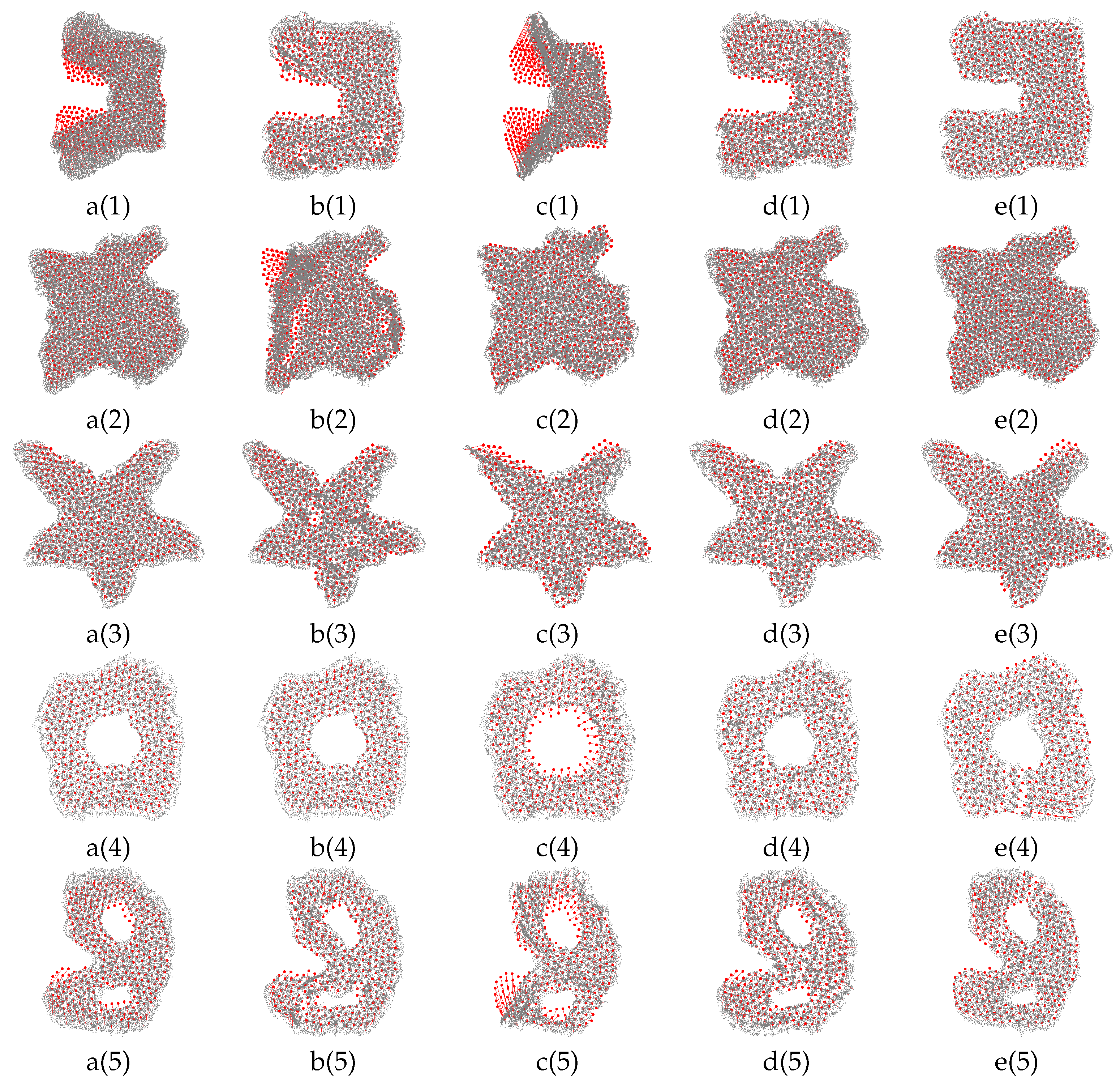
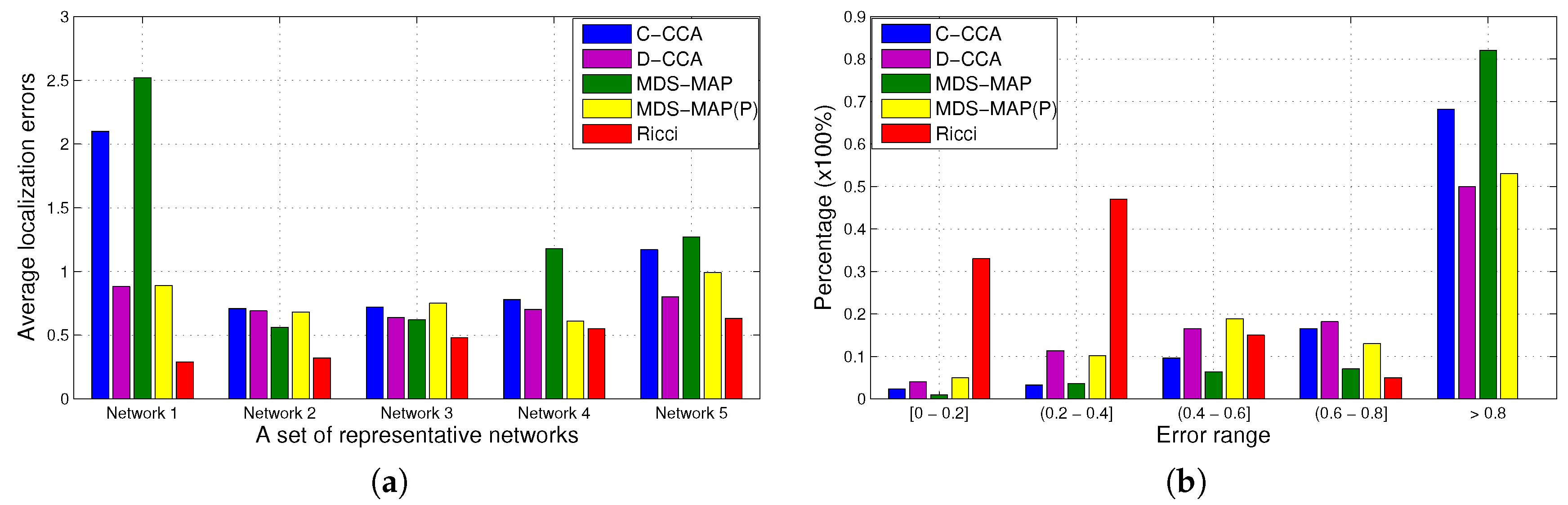
6.4. Comparison with Other Methods on Networks with Mere Connectivity

Figure 8 lists a set of representative networks with various shapes and different topologies. These networks have only connectivity information available. For these networks, we only show the original coordinates of landmark nodes marked with red color. Grey points represent the computed coordinates of sensor nodes of the networks, including landmark and non-landmark nodes, after a least square alignment with the original networks. We associate each landmark node with a red line segment, starting from its original coordinates marked with red and ending at the computed coordinates marked with grey. Clearly, the length of the line segment indicates the localization error of that node. Overall, the more and the longer the red lines are, the worse the localization performance is.
As can be observed in Figure 8a(1),c(1), C-CCA and MDS-MAP both yield large distortions for nodes on the two branches. This is because the approximated distances based on hop counts among those nodes are much longer than their actual Euclidean distances due to the reversed C shape. On the contrary, MDS-MAP(P) and D-CCA compute local maps first and then merge them into a global map. Since local maps are “smooth” and do not have large “tentacles” in general, the shortest paths are free of significant distortions. Therefore, both methods achieve better performance (i.e., less distortion and lower errors) than the centralized approaches for networks with irregular boundary conditions. This can be clearly seen in Figure 8b(1),d(1). However, if a network has a smooth boundary (e.g., Figure 8a(2)–e(2)), the shortest paths are not seriously distorted, and thus, the centralized schemes perform better since they utilize more constraints to localize the network nodes.
For networks with holes, similarly as the reversed C-shaped network, MDS-MAP(P) and D-CCA perform better (shown in Figure 8b(4),b(5),d(4),d(5)) compared with their centralized counterparts MDS-MAP and C-CCA (shown in Figure 8a(4),a(5),c(4),c(5)). However, they have to pay the cost to merge different subnetworks together.
The proposed optimal flat metric-based approach, on the contrary, achieves the least overall localization errors in all simulated scenarios as demonstrated in Figure 8e(1)–e(5). Figure 9a summarizes the average localization errors with different approaches on the models shown in Figure 8.
Figure 9b illustrates the distribution of localization errors on the reversed C-shaped network with different localization approaches. Since the results under other networks show similar statistics, we omitted them here. As can be seen, the localization errors of the optimal flat metric-based approach are nicely distributed at the lower range.

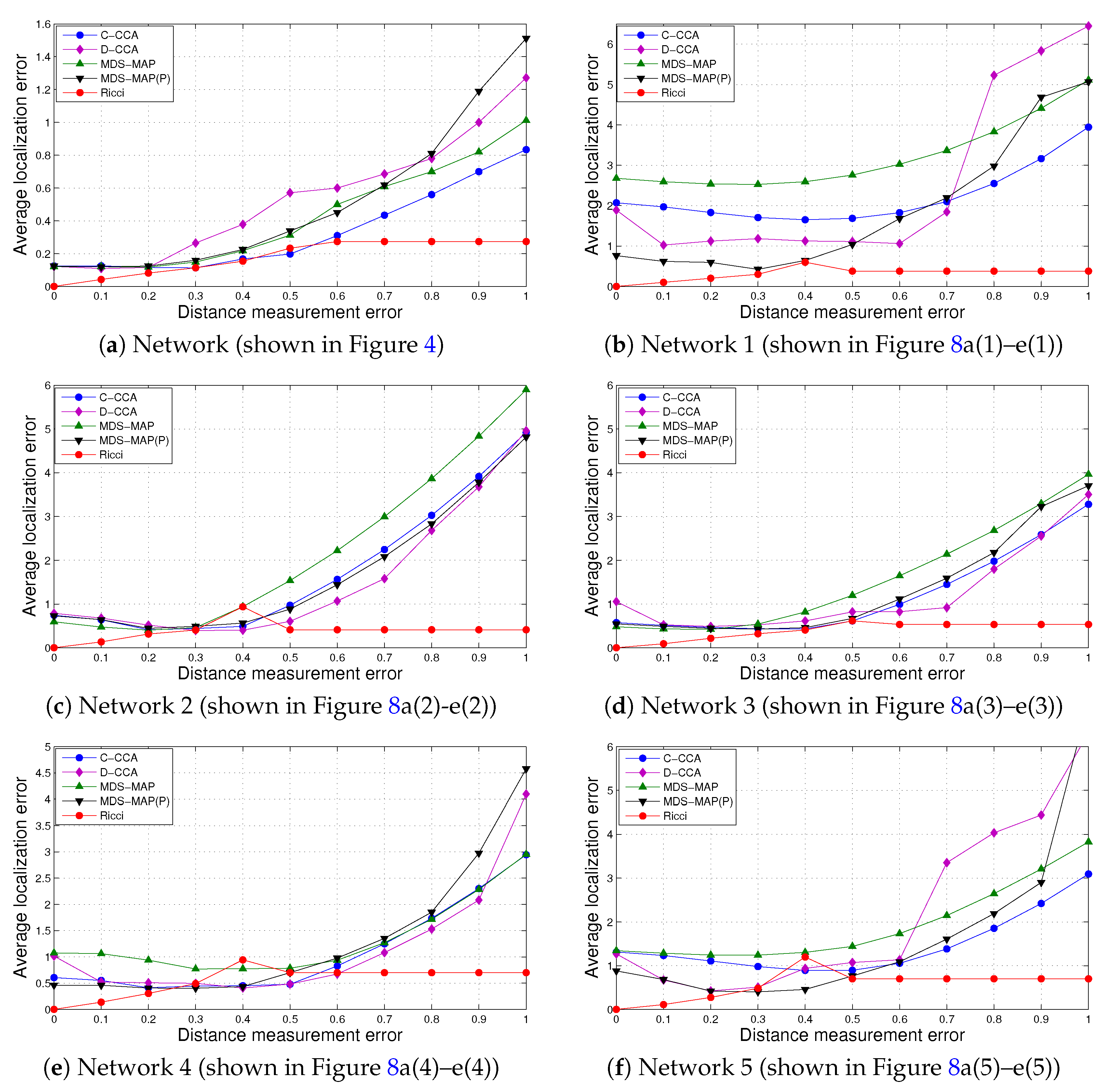
6.5. Comparison with Other Methods on Networks with Range Distance Measurements

Figure 10 summarizes the average localization errors of the proposed optimal flat metric-based approach and other methods on the networks shown in Figure 4 and Figure 8 with one-hop communication radio range distance information. Specifically, the one-hop communication radio range distance measurement error increases from 0– 100 % of the actual distance.
Figure 10 shows that when the measurement error is less than 10 % , a localized network based on the proposed algorithm is very close to the original one. When the measurement error is less than 40 % shown in Figure 10b,d, 30 % shown in Figure 10a,c and 25 % shown in Figure 10e,f, the proposed algorithm achieves the highest localization accuracy compared with other methods. However, from the other side, the proposed algorithm is more sensitive to measurement error than other localization methods. Its performance decreases with the increase of the measurement error. When the measurement error is more than 50 % , many triangles formed by three sensor nodes within their mutual communication radio range degenerate, and the measured one-hop communication radio range distances even do not satisfy the triangle inequality. We cannot take the measured distances as a legal and initial metric of the constructed mesh any more, so we have to take an average of the measured one-hop communication radio range distance as an initial metric of the mesh, which means each edge is assigned a uniform length. Such averaged distance is robust to random errors, which explaining that the performance of the proposed algorithms keeps stable when the measurement error is more than 50 % .
C-CCA and MDS-MAP, the centralized neural network-based and MDS-based approaches, on the contrary, are least sensitive to measurement error. Such random error directly affects the measured distances of pairs of nodes within the one-hop communication radio range, which is only a small portion of the distance matrix of a network. However, for a pair of nodes not within one-hop communication radio range, the longer their distance is, the smaller the random error accumulated along their path is. Therefore, we do not observe noticeable performance decline of C-CCA when the measurement error is small. The performance of C-CCA starts to decrease when the measurement error is over 40 % shown in Figure 10c,d, 50 % shown in Figure 10a,e and 70 % shown in Figure 10b,f. Similar to C-CCA, there is no noticeable performance decline of MDS-MAP when the measurement error is small. The performance of MDS-MAP starts to decrease when the measurement error is over 30 % shown in Figure 10a,c,d, 50 % shown in Figure 10b,f and 60 % shown in Figure 10e.
D-CCA and MDS-MAP(P), the distributed neural network-based and MDS-based approaches, can achieve a higher localization accuracy than their centralized counterparts when the measurement error is small. However, they are also more sensitive to measurement error than their centralized counterparts.
Combining Figure 8 and Figure 10, it is obvious that when the measurement error is more than 50 % of the actual distance, such measured one-hop communication radio range distance will not help improve localization accuracy for any of the compared localization methods including the one proposed in this paper.

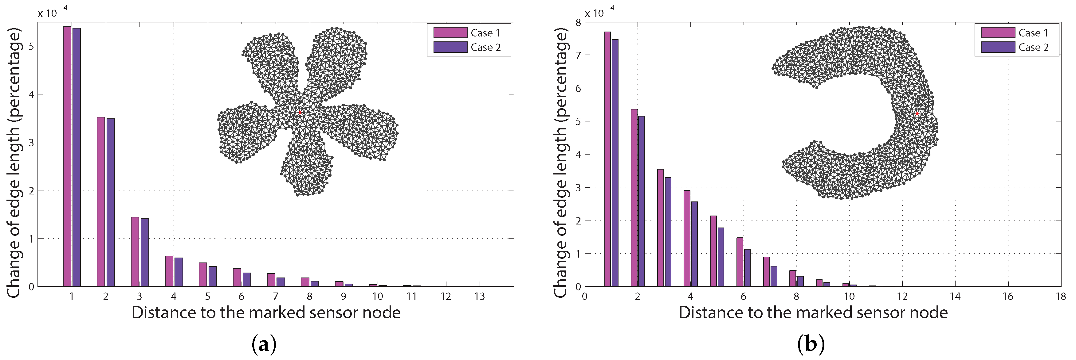
6.6. Error Propagation on Networks with One-Hop Communication Radio Range Distance Measurements
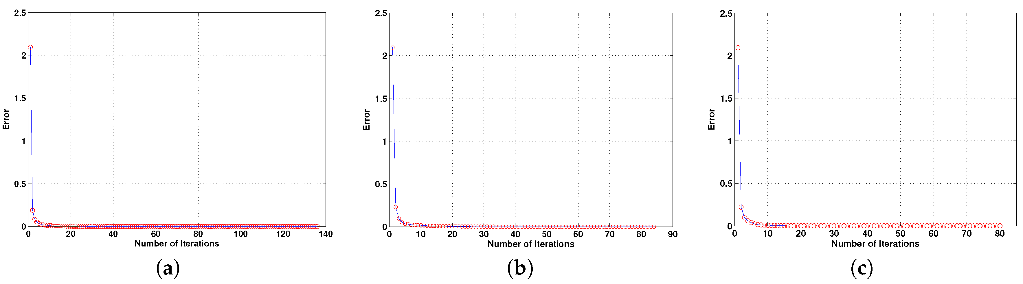
We conduct the following experiments to test the propagation rate of the measurement error resulting from bad estimation or the wrong measurement. Two networks with a constructed triangular mesh structure are shown in the top right of Figure 11a,b. If the given one-hop communication radio range distance is free of measurement error, the discrete Ricci flow-based method localizes the two networks with localization errors 1.4 × 10 5 and 1.5 × 10 5 , respectively; while if the distance measurement around one node is wrong, for example, a much slower response of a node to its neighboring nodes’ signals will result in a much longer distance approximation. The measurement error around the node will affect not just localization of this node, but also other nodes in the network (e.g., error will propagate). We introduce such measurement error at one selected node (marked with red in the two triangular networks shown in Figure 11a,b) by multiplying some constant K ( K = 2.0 for Case 1, K = 1.5 for Case 2) with the lengths of its neighboring edges, such that the node is no longer planar based on the wrong measurement. We measure the effect of the “one node measurement error” by comparing the change of the computed flat metric (edge length) with the original one. Figure 11a,b shows the distribution of the average errors of edge lengths of the two testing networks with respect to the distance to the selected node, respectively. The closer the two ending nodes of one edge are to the selected node, the bigger the distortion of the computed edge length is. It is obvious that the error propagation decreases dramatically with the increase of the distance to the distorted node. The localization errors of the two networks with distorted vertices are 0.0018 and 0.0020, respectively.

6.7. Computing Time

In our experiments, we set the step length of running discrete Ricci flow to 0.1 and the error threshold to 1 × 10 5 . Figure 12 gives the convergence rate and time using discrete Ricci flow to compute optimal flat metric for part of our simulation networks. Specifically, for the reversed C-shaped network with 3 k sensor nodes and 424 landmarks chosen, the convergence time of discrete Ricci slow is 2 s. The curvature error is less than 0.1 and 0.0004 after five and 82 iterations, respectively. For the network with one hole and 2 k sensor nodes and 283 landmarks chosen, the convergence time is 1 s. The curvature error is less than 0.1 and 0.0004 after four and 55 iterations, respectively. For the network with two holes and 2 k sensor nodes and 297 landmarks chosen, the convergence time is 1 s. The curvature error is less than 0.1 and 0.0004 after four and 48 iterations, respectively. The time of the isometric embedding of each network is no more than a few seconds. Therefore, the total computing time of a network including choosing the landmark nodes, building a triangular structure, computing the optimal flat metric and isometric embedding the network is no more than 10 s on a Dell Latitude e6420 laptop. Note that the computation is fully distributed such that each vertex node computes and exchanges information with only its neighboring vertex nodes.
We can also apply a centralized method to compute the optimal flat metric using discrete Ricci flow. Each vertex node sends its connectivity information and distance measurement within the one-hop transmission range if available to a central server. The central server can apply Newton’s method as discussed in our previous paper [29] to compute the optimal flat metric with discrete Ricci flow. Compared with the distributed method introduced in this paper, the centralized method converges in less than five iterations with the total computing time of less than 1 s for all of the testing networks.

7. Conclusions

This work proposes a novel optimal flat metric-based localization method suitable for large-scale sensor networks. The method can be proven to generate an optimal flat metric that introduces the least distortion from the initially estimated edge length. The computation is fully distributed and highly scalable with its computation time and communication cost linear to the size of the network. Extensive simulations and comparisons with other methods under various representative network settings are carried out, showing the superior performance of the proposed algorithms.

Acknowledgments

Miao Jin is partially supported by NSF CCF-1054996 and CNS-1320931. Hongyi Wu is partially supported by NSF CNS-1320931.

Author Contributions

Miao Jin designed the algorithm and wrote the paper. Su Xia did the simulations and wrote the paper. Hongyi Wu and Xianfeng David Gu analyzed the algorithm.

Conflicts of Interest

The authors declare no conflict of interest.

References

  1. Shang, Y.; Ruml, W.; Zhang, Y.; Fromherz, M.P. Localization from Mere Connectivity. In Proceedings of the 4th ACM International Symposium on Mobile ad Hoc Networking and Computing, Annapolis, MD, USA, 1–3 June 2003; pp. 201–212. [Google Scholar]
  2. Shang, Y.; Ruml, W. Improved MDS-based Localization. In Proceedings of the Twenty-Third Annual Joint Conference of the IEEE Computer and Communications Societies, Hong Kong, China, 7–11 March 2004; pp. 2640–2651. [Google Scholar]
  3. Vivekanandan, V.; Wong, V.W. Ordinal MDS-based Localization for Wireless Sensor Networks. Int. J. Sens. Netw. 2006, 1, 169–178. [Google Scholar] [CrossRef]
  4. Giorgetti, G.; Gupta, S.; Manes, G. Wireless Localization Using Self-Organizing Maps. In Proceedings of the 6th ACM International Conference on Information Processing in Sensor Networks, Cambridge, MA, USA, 25–27 April 2007; pp. 293–302. [Google Scholar]
  5. Li, L.; Kunz, T. Localization Applying An Efficient Neural Network Mapping. In Proceedings of the 1st International Conference on Autonomic Computing and Communication Systems, Rome, Italy, 28–30 October 2007; pp. 1–9. [Google Scholar]
  6. Hamilton, R.S. Three Manifolds with Positive Ricci Curvature. J. Differ. Geom. 1982, 17, 255–306. [Google Scholar] [CrossRef]
  7. Lim, H.; Hou, J. Distributed Localization for Anisotropic Sensor Networks. ACM Trans. Sens. Netw. 2009, 5, 11–37. [Google Scholar] [CrossRef]
  8. Wu, H.; Wang, C.; Tzeng, N.F. Novel Self-Configurable Positioning Technique for Multi-hop Wireless Networks. IEEE/ACM Trans. Netw. 2005, 13, 609–621. [Google Scholar]
  9. Wang, Y.; Lederer, S.; Gao, J. Connectivity-based Sensor Network Localization with Incremental Delaunay Refinement Method. In Proceedings of the IEEE INFOCOM Conference, Rio de Janeiro, Brazil, 19–25 April 2009; pp. 2401–2409. [Google Scholar]
  10. Biswas, P.; Ye, Y. Semidefinite programming for ad hoc wireless sensor network localization. In Proceedings of the 3rd ACM International Symposium on Information Processing in Sensor Networks, Berkeley, CA, USA, 26–27 April 2004; pp. 46–54. [Google Scholar]
  11. So, A.M.C.; Ye, Y. Theory of semidefinite programming for sensor network localization. In Proceedings of the Sixteenth Annual ACM-SIAM Symposium on Discrete Algorithms, Society for Industrial and Applied Mathematics, Vancouver, BC, Canada, 23–25 January 2005; pp. 405–414. [Google Scholar]
  12. Kuhn, F.; Moscibroda, T.; Wattenhofer, R. Unit disk graph approximation. In Proceedings of the 2004 ACM Joint Workshop on Foundations of Mobile Computing, Philadelphia, PA, USA, 1 October 2004; pp. 17–23. [Google Scholar]
  13. Moscibroda, T.; O’Dell, R.; Wattenhofer, M.; Wattenhofer, R. Virtual coordinates for ad hoc and sensor networks. In Proceedings of the 2004 ACM Joint Workshop on Foundations of Mobile Computing, Philadelphia, PA, USA, 1 October 2004; pp. 8–16. [Google Scholar]
  14. Basu, A.; Gao, J.; Mitchell, J.S.; Sabhnani, G. Distributed localization using noisy distance and angle information. In Proceedings of the 7th ACM International Symposium on Mobile ad Hoc Networking and Computing, Florence, Italy, 22–25 May 2006; pp. 262–273. [Google Scholar]
  15. Costa, J.A.; Patwari, N.; Hero, A.O., III. Distributed weighted-multidimensional scaling for node localization in sensor networks. ACM Trans. Sens. Netw. 2006, 2, 39–64. [Google Scholar] [CrossRef]
  16. Hamilton, R.S. The Ricci flow on surfaces. Contemp. Math. 1988, 71, 237–261. [Google Scholar]
  17. Chow, B. The Ricci flow on the 2-sphere. J. Differ. Geom. 1991, 33, 325–334. [Google Scholar] [CrossRef]
  18. Chow, B.; Luo, F. Combinatorial Ricci Flows on Surfaces. J. Differ. Geom. 2003, 63, 97–129. [Google Scholar] [CrossRef]
  19. Thurston, W.P. Geometry and Topology of Three-Manifolds. Princet. Lect. Notes 1976, 17, 1877–1954. [Google Scholar]
  20. Weintraub, S.H. Differential Forms: A Complement to Vector Calculus; Academic Press: San Diego, CA, USA, 2007. [Google Scholar]
  21. Sarkar, R.; Yin, X.; Gao, J.; Luo, F.; Gu, X.D. Greedy Routing with Guaranteed Delivery Using Ricci Flows. In Proceedings of the IEEE International Conference on Information in Sensor Networks, San Francisco, CA, USA, 13–16 April 2009; pp. 121–132. [Google Scholar]
  22. Funke, S.; Milosavljevic, N. Guaranteed-Delivery Geographic Routing Under Uncertain Node Locations. In Proceedings of the 26th IEEE International Conference on Computer Communications, Anchorage, AK, USA, 6–12 May 2007; pp. 1244–1252. [Google Scholar]
  23. Funke, S.; Milosavljevic, N. How Much Geometry Hides in Connectivity–Part II. In Proceedings of the Eighteenth Annual ACM-SIAM Symposium on Discrete Algorithms, New Orleans, LA, USA, 7–9 January 2007; pp. 958–967. [Google Scholar]
  24. Zhao, Y.; Wu, H.; Jin, M.; Xia, S. Localization in 3D Surface Sensor Networks: Challenges and Solutions. In Proceedings of the 31st Annual IEEE International Conference on Computer Communications, Orlando, FL, USA, 25–30 March 2012; pp. 55–63. [Google Scholar]
  25. Zhou, H.; Wu, H.; Xia, S.; Jin, M.; Ding, N. A Distributed Triangulation Algorithm for Wireless Sensor Networks on 2D and 3D Surface. In Proceedings of the 30th IEEE International Conference on Computer Communications, Shanghai, China, 10–15 April 2011; pp. 1053–1061. [Google Scholar]
  26. Jin, M.; Kim, J.; Gu, X. Discrete Surface Ricci Flow: Theory and Applications. Math. Surf. 2007, 4647, 209–232. [Google Scholar]
  27. Henle, M. A Combinatorial Introduction to Topology; Dover Publications: New York, NY, USA, 1994. [Google Scholar]
  28. Bettstetter, C.; Hartmann, C. Connectivity of wireless multihop networks in a shadow fading environment. Wirel. Netw. 2005, 11, 571–579. [Google Scholar] [CrossRef]
  29. Jin, M.; Kim, J.; Luo, F.; Gu, X. Discrete Surface Ricci Flow. IEEE Trans. Vis. Comput. Graph. 2008, 14, 1030–1043. [Google Scholar] [CrossRef] [PubMed]
Figure 1. Circle packing metric. (a) Flat circle packing metric on a triangular mesh; (b) circle packing metric on a triangle.
Axioms 06 00015 g001
Figure 2. (a) Dangling vertex: Vertex v 1 belongs to two disconnected boundaries with boundary edges marked with red color. After vertex split, the two boundaries are merged into one. Now, a boundary vertex belongs to one boundary only. (b) Dangling edge: Edge e 01 belongs to two disconnected boundaries with boundary edges marked with red color. After edge removal, the two boundaries are merged into one. Now, a boundary edge belongs to one boundary and is adjacent with one triangle.
Axioms 06 00015 g002
Figure 3. Short edge collapse: the operation of short edge collapse combines v a and v b to v a and removes faces f a b c and f a b d .
Axioms 06 00015 g003
Figure 4. (a) A triangular mesh with too many skinny triangles is constructed from a network based on the algorithm proposed in [25]. Its maximal r f value is close to 27. (b) After a series of short edge collapse operations, the maximal r f value of the triangular mesh is less than four.
Axioms 06 00015 g004
Figure 5. Networks with variant nodal density: (ad) The original network with increased nodal density; (eh) the localization results of our algorithm. All of the networks share the same communication radio range and are under the same transmission model. We compute the difference of each node-pair’s distances in the original and localized networks. Then, we calculate the localization error as the ratio of the average difference of node-pair’s distances and the one-hop communication radio range. Specifically, the average nodal degrees for networks shown in (ad) increase with d = 9.4 , d = 12.6 , d = 15.2 , d = 18.5 , respectively. The localization errors of networks shown in (ad) decrease with 0.514 , 0.322 , 0.28 , 0.246 , respectively. (eh) show the corresponding localization results. The localization error decreases with the increase of nodal density.
Axioms 06 00015 g005
Figure 6. Networks with different transmission models: (ad) the original networks with different transmission models that result in different nodal degrees and constructed triangular meshes; (eh) the embedding results of our algorithm. All of the networks have the same number of nodes and the same communication range. (a) Unit disk graph (UDG) model with transmission range of one and localization error 0.25 in (e); (b) Quasi-UDG model with α = 0.75 and ρ = 0.5 and localization error 0.34 in (f); (c) log norm model with μ = 0.5 and ρ = 4 and localization error 0.42 in (g); (d) probability model with p = 0.65 and localization error 0.43 in (h).
Axioms 06 00015 g006
Figure 7. Network with non-uniform node distribution: (a) The original network with non-uniform node distribution. The nodal degrees range from 11.3 18.7 . (b) The localization result of our algorithm with the localization error 0.46 .
Axioms 06 00015 g007
Figure 8. Comparison with other methods on networks with mere connectivity. (a(1)a(5)) C-CCAscheme; (b(1)b(5)): D-CCA scheme; (c(1)c(5)) multi-dimensional scaling (MDS)-MAPscheme; (d(1)d(5)) MDS-MAP(P) scheme; (e(1)e(5)) Ricci scheme. A red line segment is drawn for each node, starting from the real coordinates marked with red and ending at the computed coordinates marked with grey.
Axioms 06 00015 g008
Figure 9. (a) Comparison of the average localization errors of different methods on the networks shown in Figure 8 with mere connectivity information: Network 1 shown in Figure 8a(1)–e(1), Network 2 shown in Figure 8a(2)–e(2), Network 3 shown in Figure 8a(3)–e(3), Network 4 shown in Figure 8a(4)–e(4) and Network 5 shown in Figure 8a(5)–e(5). (b) The distribution of connectivity-based localization errors on the reversed C-shaped network with different approaches: C-CCA, D-CCA, MDS-MAP, MDS-MAP(P) and Ricci.
Axioms 06 00015 g009
Figure 10. Comparison of average localization errors of different methods on networks shown in Figure 4 and Figure 8 with one-hop communication radio range distance measurement errors increased from 0– 100 % .
Axioms 06 00015 g010
Figure 11. The error of the computed edge length decreases dramatically with its distance to the distorted node marked with red.
Axioms 06 00015 g011
Figure 12. Convergence rate of discrete surface Ricci flow applied to compute the optimal flat metric of networks, with step length 0.1 and error threshold 1 × 10 5 . (a) A reversed C-shaped network with 424 landmarks: the convergence time is 2 s. (b) A network with one hole and 283 landmarks: the convergence time is 1 s. (c) A network with two holes and 297 landmarks: the convergence time is 1 s.
Axioms 06 00015 g012
Table 1. Table of notation.
SymbolExplanation
B 0 the longest boundary of M
B i the i-th boundary of M
bthe number of boundaries of M
Eedges of M
e i j an edge belonging to E with two ending vertices v i and v j
e n the number of edges of M
Ftriangle faces of M
f i j k a triangle face belonging to F with vertices v i , v j , and v k
f n the number of triangle faces of M
K i the discrete Gaussian curvature of v i V
K ¯ i the target Gaussian curvature of v i V
L i a shortest path between the initiator of B i and B 0
l i j the length of e i j
Ma triangulated surface (or mesh in short) embedded in R 3
M the boundary of M
r f i j k a ratio between the longest and shortest edge lengths of f i j k
tthe time
u i the logarithm of γ i of v i
Vvertices of M
v n the number of vertices of M
v i a vertex belonging to V with id i
θ i j k the corner angle attached to vertex v i in face f i j k
γ i the radius of a circle associated with v i
Γ the radius function assigned at M
ϕ i j weight of e i j (the intersection angle of two circles centered at v i and v j )
Φ the weight function assigned at M
( Γ , Φ ) circle packing metric of M
χ ( M ) the Euler characteristic number of M
δ the step length computing optimal flat metric
ϵ the threshold of curvature error computing optimal flat metric

