Risk-Controlling Predictive Sets for Time-Series Events Under Selective Observation with Finite-Sample Guarantees

Abstract

Selective labels create a support failure for prediction along dependent stochastic processes: alert-triggered events are observed, whereas silent periods are usually unlabeled. We model this mechanism as predictable inclusion on a filtered probability space and show that population risk is non-identifiable when any silent region has zero labeling probability. Selective-observation weighted risk control (SOWRC) combines alert labels with randomized audits through Horvitz–Thompson losses and a martingale-mixture boundary. It provides finite-sample calibration-population control under arbitrary temporal dependence subject to predictable design choices, conditional ignorability, positivity, bounded losses, and deterministic design envelopes, together with a prospective guarantee under an externally certified deployment-drift envelope and explicit error allocation. Extensions cover anytime monitoring, multiple losses, adaptive budgets, and estimated propensities. Synthetic maintenance and financial studies, a complete-log replay on a real dependent sensor series with 100 audit-mask replications, and 4000 selection-level validation runs demonstrate support recovery and conservative probabilistic risk control on deterministic threshold grids.

1. Introduction

Set-valued forecasts are increasingly used when a single point prediction is not sufficiently reliable for an operational decision. A maintenance platform may need a set of plausible fault classes before dispatching a technician, while a financial surveillance system may need a set of possible risk states before escalating an alert. From a probability-theoretic viewpoint, these systems generate dependent stochastic processes observed through a history-dependent labeling mechanism. Conformal risk control supplies a model-agnostic route from scores to sets whose loss is controlled at a user-specified level [1]. A complementary stochastic-process perspective studies updating when information is restricted [2], while online selective conformal procedures control false coverage statements after data-dependent reporting [3]. Yet most existing guarantees presume that the calibration labels represent the population on which risk will be evaluated.

Thresholded event systems violate this premise in a particularly severe way. Labels are typically collected after an alarm score crosses a prescribed level, whereas the much larger collection of sub-threshold periods remains unannotated. The resulting sample is not merely imbalanced; it is selected by a history-dependent mechanism that can be correlated with both the prediction score and the future event. Online conformal methods adapt to distribution shift [4], and multivariate time-series sets account for structured forecast errors [5], but neither contribution alone identifies the population risk hidden in the silent region. Stochastic-process diagnostics in Axioms likewise illustrate that inferential conclusions depend on which trajectory functionals are observed [6].

Dependence creates a second difficulty. Time-series events may be driven by latent regimes, persistent covariates, or feedback from past alerts. Non-exchangeable conformal methods quantify penalties caused by dependence [7], while Markov-specific analyses connect coverage gaps with mixing times [8]. Multi-horizon procedures exploit structured residuals [9]. These developments are important, but they usually assume that all calibration responses, or an exchangeability-preserving subset, are observed. In the present problem, temporal dependence and missing labels interact: the same history that raises the alert probability also changes the conditional event risk.

A natural remedy is to supplement alert-triggered labels with an auxiliary unselected stream. Examples include a small random audit of silent periods, complete historical sensor logs available for an earlier machine fleet, or a retrospective database in which outcomes were recorded independently of the alert rule. Partially observed point-process models illustrate how an auxiliary observation phase can restore information about hidden events [10]. However, the statistical role of such a stream in finite-sample predictive risk control has not been characterized. In particular, it is unclear which support condition is indispensable, how the two streams should be combined, and which guarantee survives arbitrary temporal dependence.

Recent time-series conformal methods provide complementary ingredients. Adaptive bands can track heterogeneous trajectories [11]; decomposition can separate components with different exchangeability properties [12]; and multi-step online calibration can regulate aggregate error [13]. Stochastic models with mean reversion further show how persistent latent dynamics alter stationary behavior [14]. These methods motivate history-sensitive weighting, but they do not address a selection probability that may be exactly zero below an operational threshold. That zero-probability region is the central identification obstacle studied here.

The proposed framework, called selective-observation weighted risk control (SOWRC), treats alert and audit labels as one predictable inclusion process on a filtered probability space. It estimates candidate losses by a Horvitz–Thompson transform and calibrates a nested predictive set with a simultaneous martingale-mixture upper boundary. The resulting probability guarantee is driven by conditional unbiasedness and supermartingale concentration rather than exchangeability, so the construction accommodates arbitrary temporal dependence within the observed trajectory. It connects with automatically adaptive risk control [15], label-robust conformal inference [16], and recent distribution-generalization theory under hidden confounding [17]. Its sequential layer follows modern confidence-sequence and e-value principles [18,19]. Covariate-shift systems [20] motivate explicit treatment of support, while recent probabilistic studies of hydrological risk [21] and Gaussian-product extremes [22] emphasize the importance of calibrated tail decisions.

Our first contribution is a probability-theoretic impossibility result: if a silent region has zero inclusion probability, observationally equivalent stochastic laws can have different population risks. Our second contribution is a finite-sample calibration theorem on a threshold grid fixed before labels are inspected. It separates the pointwise validity of any bounded loss from the additional monotonicity and safe-terminal conditions required for data-dependent nested-set selection. Our third contribution is a prospective theorem with explicit error accounting: future-horizon risk is controlled when an external deployment-drift certificate links the future population to the certified calibration population, and the certificate’s own failure probability is added to the calibration error. Further results cover multiple losses, adaptive budgets, estimated propensities, and oracle efficiency. The framework complements application-oriented risk control [23] and transfer conformal inference [24].

The paper also clarifies the scope of its guarantees. Covariate-shift procedures require source–target support overlap [20]; beyond-exchangeability methods reweight complete calibration samples [25]; and adaptive conformal prediction tracks errors as labels arrive [26]. Recent theory explains when split conformal inference can remain effective under temporal dependence [27], while post-training adaptive conformal prediction addresses structured missingness in incomplete time series [28]. Distribution-free risk-controlling sets [29] and modern conformal tutorials [30] provide the broader baseline. SOWRC addresses the different obstacle of zero observation support. Its arbitrary-dependence theorem certifies the weighted calibration population; prospective use additionally requires a certified drift envelope and its own error budget, which cannot be removed without further temporal structure.

The identification layer is also connected to classical unequal-probability sampling and missing-data theory. Horvitz–Thompson weighting recovers population means when inclusion probabilities are positive and known [31], and inverse-probability methods formalize the same positivity/ignorability requirements under missingness [32]. The contribution here is not a new claim that inverse weighting needs positivity. Rather, we embed that requirement in a history-adapted time-series prediction-set problem, prove an explicit zero-support impossibility result for the predictive risk target, and combine the recovered losses with a finite-sample martingale certificate that remains valid without exchangeability or mixing-rate assumptions, subject to the stated predictability and ignorability conditions.

The remainder is organized as follows. Section 2 formulates selective observation and proves non-identifiability without support. Section 3 develops SOWRC and establishes the core finite-sample theorem. Section 4 treats time-uniform control, multiple losses, and adaptive budgets. Section 5 studies robustness and efficiency. Section 6 gives numerical implementation and reproducibility details. Section 7 reports synthetic and complete-log experiments. Section 8 concludes and presents three future directions.

Table 1. Main symbols and definitions.

Symbol	Definition
t	The time index.
n	The fixed calibration horizon.
H	The prospective deployment horizon.
$X_t$	The observed covariate vector at time t.
$Y_t$	The event label at time t.
${\mathcal{F}}_t$	The post-label information available after time t.
${\mathcal{H}}_t$	The pre-label history $\sigma ({\mathcal{F}}_{t-1},X_t)$.
$S_t$	The alert-selection indicator.
$A_t$	The auxiliary-audit indicator.
$I_t$	The label-inclusion indicator.
$q_t$	The conditional probability that the label is included.
$\mathcal{Y}$	The finite label space.
$C_{t,\lambda }\left(x\right)$	The nested predictive set at threshold $\lambda$.
$\lambda$	The threshold controlling prediction-set size.
$L_t\left(\lambda \right)$	The bounded predictive loss.
$R_t\left(\lambda \right)$	The conditional population risk.
$a_{t,n}$	A horizon-indexed fixed-horizon weight, such as Equation (14).
$a_t$	A single predictable weight sequence used in the anytime setting.
$c_n,b_n$	Deterministic design envelopes for a fixed terminal horizon.
$c,b$	Global design envelopes used for time-uniform validity.
$Z_t\left(\lambda \right)$	The inverse-inclusion weighted observed loss.
$A_n$	The cumulative history weight.
$U_n(\lambda ;\delta )$	The finite-sample upper risk boundary.
${\alpha }_t$	The predictable risk budget.
$\Lambda$	The threshold grid fixed before labels are inspected.
${\widehat{\Delta }}_{n,H}$	The certified calibration-to-deployment drift envelope.
${\delta }_{\mathrm{dep}}$	The failure probability of the drift certificate.
${\rho }_t$	The auxiliary-audit probability.
$q_{\min }$	The deterministic lower bound on label-inclusion probability.

summarizes the notation used throughout the paper.

2. Problem Formulation and Identification

2.1. Time-Series Prediction Under Selective Labels

Let $(\Omega ,\mathcal{A},\mathbb{P})$ carry a filtered process ${\left\{(X_t,Y_t)\right\}}_{t\ge 1}$, where $X_t\in \mathcal{X}$ and $Y_t\in \mathcal{Y}=\{1,\dots ,m\}$. The post-label filtration and pre-label history are

$${\mathcal{F}}_t=\sigma \left({\mathcal{F}}_{t-1},X_t,S_t,A_t,I_t,I_t{Y}_t\right),$$

(1)

$${\mathcal{H}}_t=\sigma ({\mathcal{F}}_{t-1},X_t).$$

(2)

A black-box predictor produces ${\mathcal{H}}_t$-measurable class probabilities $p_t(y\mid X_t)$ and a nonconformity score

$$r_t(x,y)=1-p_t(y\mid x).$$

(3)

For a threshold $\lambda \in [0,1]$, define the nested set

$$C_{t,\lambda }\left(x\right)=\{y\in \mathcal{Y}:r_t(x,y)\le \lambda \}.$$

(4)

Nestedness gives

$${\lambda }_1\le {\lambda }_2⟹C_{t,{\lambda }_1}\left(x\right)\subseteq C_{t,{\lambda }_2}\left(x\right).$$

(5)

The principal loss is event miscoverage,

$$L_t\left(\lambda \right)=\mathbf{1}\{Y_t\notin C_{t,\lambda }\left(X_t\right)\}=\mathbf{1}\{r_t(X_t,Y_t)>\lambda \}.$$

(6)

The pointwise concentration analysis also permits any ${\mathcal{H}}_t\vee \sigma \left(Y_t\right)$-measurable loss satisfying

$$0\le L_t^{\left(k\right)}\left(\lambda \right)\le 1,k=1,\dots ,K.$$

(7)

Data-dependent selection over a nested family additionally requires monotonicity and a certified safe terminal action, stated in Assumption 3.

The operational alert rule is represented by $S_t\in \{0,1\}$. Its conditional probability may depend on the full observed history,

$${\pi }_t=\mathbb{P}(S_t=1\mid {\mathcal{H}}_t).$$

(8)

An auxiliary audit independently requests a label with conditional probability

$${\rho }_t=\mathbb{P}(A_t=1\mid {\mathcal{H}}_t).$$

(9)

A label is observed when either channel fires:

$$I_t=1-(1-S_t)(1-A_t).$$

(10)

Under conditional independence of $S_t$ and $A_t$ given ${\mathcal{H}}_t$, the inclusion propensity is

$$q_t=\mathbb{P}(I_t=1\mid {\mathcal{H}}_t)={\pi }_t+{\rho }_t-{\pi }_t{\rho }_t.$$

(11)

The target is not alert-conditional risk. It is the weighted population risk over all periods,

$${\overline{R}}_n\left(\lambda \right)={\displaystyle \frac{1}{A_n}}{\sum }_{t=1}^n{a}_t{R}_t\left(\lambda \right),A_n={\sum }_{t=1}^n{a}_t,$$

(12)

where $a_t>0$ is ${\mathcal{H}}_t$-measurable and

$$R_t\left(\lambda \right)=\mathbb{E}[L_t\left(\lambda \right)\mid {\mathcal{H}}_t].$$

(13)

For a fixed terminal horizon, exponential forgetting is obtained with

$$a_{t,n}\left(\gamma \right)=exp\{-\gamma (n-t)\},\gamma \ge 0.$$

(14)

The second index emphasizes that these weights are redefined for a fixed-horizon target; the anytime result in Section 4.1 instead uses one predictable weight sequence satisfying global design bounds.

Four risk objects are kept distinct throughout the revision. The one-step conditional risk $R_t\left(\lambda \right)$ is a history-specific conditional expectation. The calibration-population risk ${\overline{R}}_n\left(\lambda \right)$ is the weighted finite-horizon target certified by Theorem 2. The complete-label test risk used in Section 7 is an empirical diagnostic on a held-out, fully revealed segment and is not itself a theorem target. Finally, the operational or deployment risk ${\overline{R}}_{n,H}^{\mathrm{dep}}\left(\lambda \right)$ concerns future periods and is covered only after the additional drift condition in Assumption 4.

Table 2. Risk quantities used in the manuscript and their logical status.

Quantity	Definition/Location	Interpretation
Conditional risk $R_t\left(\lambda \right)$	Equation (13)	History-specific risk before the current label is revealed.
Calibration-population risk ${\overline{R}}_n\left(\lambda \right)$	Equation (12)	Finite-horizon weighted population target controlled by Theorem 2.
Complete-label test risk	Section 7	Empirical diagnostic computed only because the experimental test segment is fully revealed.
Deployment risk ${\overline{R}}_{n,H}^{\mathrm{dep}}\left(\lambda \right)$	Equation (56)	Future operational target; controlled only with a certified drift envelope.

summarizes these four risk quantities and their logical status.

2.2. Assumptions and an Impossibility Boundary

Assumption 1

(Conditional ignorability). For every t, inclusion is conditionally independent of the label given the pre-label history:

$$I_t\perp Y_t\mid {\mathcal{H}}_t.$$

(15)

Equivalently,

$$\mathbb{P}(I_t=1\mid {\mathcal{H}}_t,Y_t)=q_t.$$

(16)

Assumption 2

(Audit positivity). There exists $q_{\min }>0$ such that

$$q_t\ge q_{\min }almostsurelyforallt.$$

(17)

Assumption 1 allows arbitrary temporal dependence and selection based on observed history. It excludes label-dependent annotation after conditioning on that history. Assumption 2 is supplied by the audit stream; for a deterministic threshold alert, it is enough to choose ${\rho }_t\ge {\rho }_{\min }>0$.

The phrase “arbitrary temporal dependence” refers only to the absence of an exchangeability, independence, or mixing-rate requirement for the observed trajectory. It does not remove the structural conditions used by the proof: the alert/audit decision and any history weights must be predictable, inclusion must satisfy conditional ignorability, losses must be bounded, and a positive inclusion floor is required. Conditional ignorability is not nonparametrically testable from selectively observed labels alone. In practice, the most defensible design is to generate the audit request by external randomization before the current outcome is known. If an alerting or annotation system uses latent same-period information that is not recorded in ${\mathcal{H}}_t$, the assumption can fail and the theorem should not be invoked without enlarging the recorded history or performing a sensitivity analysis.

Table 3. Core assumptions, associated guarantees, and empirical assessability.

Assumption/Design Condition	Role	Main Result	Assessability
Predictability of $S_t,A_t,a_t$	Choices are made before the current hidden label is revealed.	Lemma 1, Theorems 2 and 3	Checkable from system timing and logs.
Conditional ignorability	Makes inverse-inclusion loss conditionally unbiased.	Equations (25) and (26)	Not fully testable from observed labels; strengthened by randomized audits.
Positivity $q_t\ge q_{\min }>0$	Restores identification and bounds inverse weights.	Theorem 1; Theorem 2	Directly checkable when the audit policy is randomized and logged.
Bounded loss and design envelopes	Enables finite-sample martingale concentration.	Lemma 1	Checkable by construction.
Nested safety	Justifies data-dependent threshold selection and safe fallback.	Equation (54)	Checkable from the loss and terminal set definition.
Certified drift envelope	Links calibration risk to future deployment risk.	Corollary 1	Requires an external validation mechanism or process bound.

summarizes the role, guarantee, and assessability of the core assumptions and design conditions.

For an arbitrary predictable set-valued rule $C_{1:n}$, write its weighted population miscoverage as

$${\mathcal{R}}_n\left(C_{1:n}\right)={\displaystyle \frac{1}{A_n}}{\sum }_{s=1}^n{a}_s\mathbb{E}[\mathbf{1}\{Y_s\notin C_s\}\mid {\mathcal{H}}_s].$$

(18)

Theorem 1

(Non-identifiability without silent-region support). Fix a horizon n and suppose that, for some $t\le n$, an event $G\in {\mathcal{H}}_t$ satisfies $\mathbb{P}\left(G\right)>0$ and $q_t=0$ on G. Let $C_t$ be the set reported before observing $Y_t$. If 

$$\mathbb{P}\{G,⌀\ne C_t⊊\mathcal{Y}\}>0,$$

(19)

there exist two time-series laws $P_0$ and $P_1$ with the same distribution of the complete observed trajectory through time n but with ${\mathcal{R}}_{n,P_0}\left(C_{1:n}\right)\ne {\mathcal{R}}_{n,P_1}\left(C_{1:n}\right)$. If instead $\mathbb{P}\{G,C_t=⌀\}>0$, the rule incurs unit conditional miscoverage on that event under every compatible label law. Consequently, uniform control at arbitrarily small levels forces the full label space on every zero-inclusion region.

Proof. 

Because $\mathcal{Y}$ is finite, Equation (19) implies that there is a label $y^{★}\in \mathcal{Y}$ for which

$$p_{★}=\mathbb{P}\{G,⌀\ne C_t,y^{★}\notin C_t\}>0.$$

(20)

Let U denote the procedure’s independent random seed and augment the pre-label history by $\sigma \left(U\right)$; equivalently, condition on U and average at the end. Construct $P_0$ and $P_1$ on a common covariate, selection, and randomization process. Outside G, let their conditional label laws coincide. On G, set $Y_t=y^{★}$ under $P_1$. Under $P_0$, choose a measurable selector $y_0\left(C_t\right)\in C_t$ whenever $C_t$ is nonempty; on $C_t=⌀$, use the same fixed label under both laws. The output is measurable before $Y_t$ is generated, and the label is never revealed on G. The construction is existential: the model class permits arbitrary temporal dependence, but it does not require every admissible law to make future observables depend on the hidden $Y_t$. We therefore choose, under both $P_0$ and $P_1$, the same post-t transition kernel for the observable coordinates conditional on the recorded history, with that kernel not depending on the unrevealed value of $Y_t$ on G. This defines two legitimate members of the stated model class. The argument does not claim that one may alter $Y_t$ while holding fixed an arbitrary pre-specified data-generating mechanism in which $Y_t$ causally changes later covariates.

Since $q_t=0$ on G, the observed variable $I_t{Y}_t$ is absent there. Under the paired laws just constructed, induction over the common observable transition kernels therefore gives, for every measurable function h of the observed trajectory,

$${\mathbb{E}}_{P_0}\left[h\left({\mathcal{F}}_n\right)\right]={\mathbb{E}}_{P_1}\left[h\left({\mathcal{F}}_n\right)\right].$$

(21)

On the event in Equation (20), the time-t miscoverage under $P_1$ equals one and that under $P_0$ equals zero. Hence,

$${\mathbb{E}}_{P_1}\left[\mathbf{1}\{Y_t\notin C_t\}{\mathbf{1}}_G\right]-{\mathbb{E}}_{P_0}\left[\mathbf{1}\{Y_t\notin C_t\}{\mathbf{1}}_G\right]\ge p_{★}>0.$$

(22)

All other time contributions can be chosen equal, so positive weighting yields

$${\mathcal{R}}_{n,P_1}\left(C_{1:n}\right)-{\mathcal{R}}_{n,P_0}\left(C_{1:n}\right)\ge {\displaystyle \frac{a_t{p}_{★}}{A_n}}>0.$$

(23)

Thus the observed law cannot determine the target risk. An empty output on a positive-probability subset of G has miscoverage of one regardless of the hidden label. Uniform control at every arbitrarily small level therefore rules out both empty and nonempty proper outputs, forcing $C_t=\mathcal{Y}$ almost surely on every zero-inclusion region.    □

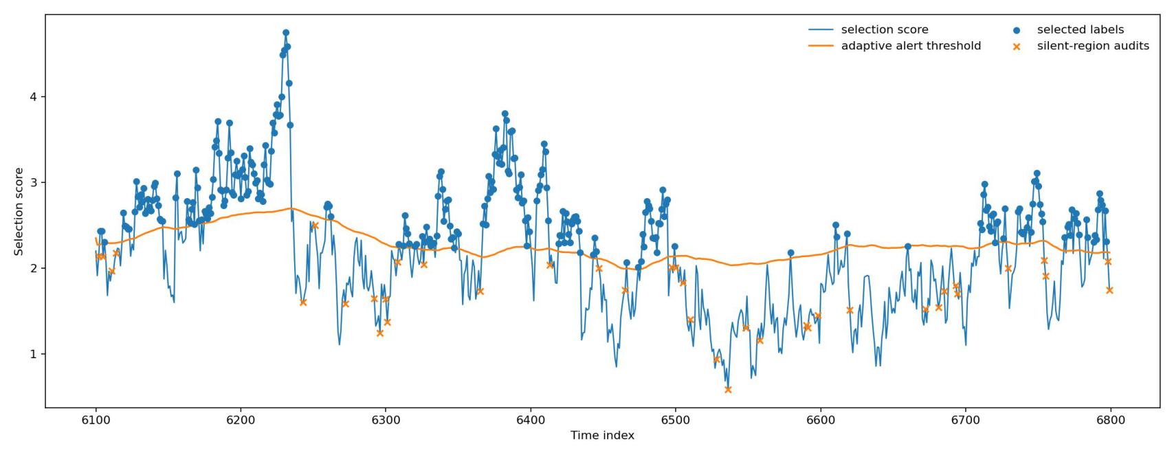
Figure 1 visualizes the support issue. Alert labels concentrate above a moving threshold, while the audit channel places sparse labels throughout the silent region. Those audited points are not intended to make the sample balanced. Their role is more fundamental: they make every history stratum observable with positive probability, which turns an unidentified target into an estimable population risk.

Figure 1 was redrawn with a more reactive, lagged-score threshold so that history dependence is visually apparent rather than nearly indistinguishable from a constant cutoff. Orange circles arise when the score exceeds the predictable adaptive threshold, whereas green crosses are randomized audits in silent periods. The threshold is computed only from information available before the current label, so its visible movement illustrates allowed adaptive selection without violating predictability. The purpose of the audits is to support recovery, not class balancing.

Remark 1.

The impossibility theorem is not a statement that selective data are unusable. It isolates the exact failure mode: an unobserved region with zero inclusion probability. A small randomized audit is therefore qualitatively different from merely collecting more alert labels. Additional selected labels reduce variance inside the alert region, whereas audits restore identification across the population support and make any finite-sample population guarantee logically possible.

3. Selective-Observation Weighted Risk Control

3.1. Unbiased Loss Recovery

Define the inverse-inclusion loss

$$Z_t\left(\lambda \right)={\displaystyle \frac{I_t}{q_t}}{L}_t\left(\lambda \right).$$

(24)

Conditional ignorability gives the identity

$$\mathbb{E}[Z_t\left(\lambda \right)\mid {\mathcal{H}}_t,Y_t]=L_t\left(\lambda \right),$$

(25)

and therefore

$$\mathbb{E}[Z_t\left(\lambda \right)\mid {\mathcal{H}}_t]=R_t\left(\lambda \right).$$

(26)

The empirical weighted risk is

$${\widehat{R}}_n\left(\lambda \right)={\displaystyle \frac{1}{A_n}}{\sum }_{t=1}^n{a}_t{Z}_t\left(\lambda \right).$$

(27)

Its martingale difference is

$$D_t\left(\lambda \right)=a_t\{Z_t\left(\lambda \right)-R_t\left(\lambda \right)\}.$$

(28)

By Assumption 2,

$$|D_t\left(\lambda \right)|\le {\displaystyle \frac{a_t}{q_{\min }}}.$$

(29)

A predictable conditional variance proxy is

$$v_t\left(\lambda \right)=\mathbb{E}[D_t^2\left(\lambda \right)\mid {\mathcal{H}}_t]\le a_t^2\mathbb{E}\left[{\displaystyle \frac{L_t\left(\lambda \right)}{q_t}}|{\mathcal{H}}_t\right]\le {\displaystyle \frac{a_t^2}{q_{\min }}}.$$

(30)

Let

$$V_n\left(\lambda \right)={\sum }_{t=1}^n{v}_t\left(\lambda \right).$$

(31)

When a variance-sensitive closed-form boundary is used, fix, before the labels are inspected, a deterministic envelope ${\mathcal{V}}_n\left(\lambda \right)$ satisfying

$$V_n\left(\lambda \right)\le {\mathcal{V}}_n\left(\lambda \right)\mathrm{almost}\mathrm{surely}.$$

(32)

For the fixed calibration horizon, choose deterministic design envelopes $c_n,b_n>0$ such that

$$a_t\le c_n,{\displaystyle \frac{a_t}{q_t}}\le b_n\mathrm{almost}\mathrm{surely}\mathrm{for}t\le n.$$

(33)

For example, if $a_t\le a_{\max ,n}$ by design, then $c_n=a_{\max ,n}$ and $b_n=a_{\max ,n}/q_{\min }$ are valid. Using deterministic envelopes, rather than maxima depending on future random histories, is essential for the sequential conditional-expectation argument below.

Lemma 1

(Conditional exponential bound). For $0\le \eta <3/b_n$,

$$\mathbb{E}\left[exp\left\{\eta D_t\left(\lambda \right)-{\displaystyle \frac{{\eta }^2{v}_t\left(\lambda \right)}{2(1-\eta b_n/3)}}\right\}|{\mathcal{H}}_t\right]\le 1.$$

(34)

Proof. 

Condition on ${\mathcal{H}}_t$. By the definition of $D_t\left(\lambda \right)$, Equation (29), and the deterministic design envelope $a_t/q_{\min }\le b_n$ in Equation (33), we have $|D_t\left(\lambda \right)|\le b_n$. Expanding the exponential and using $k!\ge 2·3^{k-2}$ for $k\ge 2$ gives

$$\mathbb{E}[e^{\eta D_t}\mid {\mathcal{H}}_t]\le 1+{\displaystyle \frac{{\eta }^2{v}_t}{2}}{\sum }_{j=0}^{\infty }{(\eta b_n/3)}^j.$$

(35)

The geometric series equals ${(1-\eta b_n/3)}^{-1}$. Since $1+x\le e^x$,

$$\mathbb{E}[e^{\eta D_t}\mid {\mathcal{H}}_t]\le exp\left\{{\displaystyle \frac{{\eta }^2{v}_t}{2(1-\eta b_n/3)}}\right\}.$$

(36)

Rearranging proves the stated conditional inequality.    □

For a fixed threshold, Lemma 1 and the deterministic envelope in Equation (32) give

$$B_n(\delta ,\lambda )={\displaystyle \frac{\sqrt{2{\mathcal{V}}_n\left(\lambda \right)log(1/\delta )}}{A_n}}+{\displaystyle \frac{b_{n}log(1/\delta )}{3A_n}}.$$

(37)

If no refined deterministic variance envelope is available, Equation (30) gives the safe choice ${\mathcal{V}}_n\left(\lambda \right)={\sum }_{t=1}^n{a}_t^2/q_{\min }$ and hence

$${\overline{B}}_n\left(\delta \right)=\sqrt{{\displaystyle \frac{2log(1/\delta ){\sum }_{t=1}^n{a}_t^2/q_{\min }}{A_n^2}}}+{\displaystyle \frac{c_{n}log(1/\delta )}{3q_{\min }{A}_n}}.$$

(38)

A plug-in expression based on the unknown realized $V_n\left(\lambda \right)$ is not used, because optimizing a fixed-time exponential bound with a random unaccounted variance term would require an additional self-normalization argument. The deterministic safe bound is nonasymptotic but can be conservative. We therefore derive an observable risk-adaptive boundary that avoids estimating $V_n$.

3.2. Observable Martingale-Mixture Boundary

Write the cumulative target and its Horvitz–Thompson estimate as

$${\mu }_n\left(\lambda \right)=A_n{\overline{R}}_n\left(\lambda \right),{\widehat{\mu }}_n\left(\lambda \right)=A_n{\widehat{R}}_n\left(\lambda \right).$$

(39)

For the lower-deviation increment

$$H_t\left(\lambda \right)=a_t\{R_t\left(\lambda \right)-Z_t\left(\lambda \right)\}=-D_t\left(\lambda \right),$$

(40)

we have

$$H_t\left(\lambda \right)\le a_t\le c_n,\mathbb{E}[H_t^2\left(\lambda \right)\mid {\mathcal{H}}_t]\le {\displaystyle \frac{a_t^2{R}_t\left(\lambda \right)}{q_t}}\le b_n{a}_t{R}_t\left(\lambda \right).$$

(41)

For $0<\eta <3/c_n$, define

$$g_{c_n}\left(\eta \right)={\displaystyle \frac{{\eta }^2}{2(1-\eta c_n/3)}},{\kappa }_n\left(\eta \right)=\eta -b_n{g}_{c_n}\left(\eta \right).$$

(42)

Whenever ${\kappa }_n\left(\eta \right)>0$, keep the terminal-horizon envelopes $c_n,b_n$ fixed and, for $0\le k\le n$, define the triangular process

$$E_{k\mid n}(\lambda ,\eta )=exp\left\{{\kappa }_n\left(\eta \right){\sum }_{t=1}^k{a}_t{R}_t\left(\lambda \right)-\eta {\sum }_{t=1}^k{a}_t{Z}_t\left(\lambda \right)\right\}.$$

(43)

Conditional Bernstein control makes $\{E_{k\mid n}:0\le k\le n\}$ a nonnegative supermartingale. Its terminal value is $exp\{{\kappa }_n\left(\eta \right){\mu }_n-\eta {\widehat{\mu }}_n\}$. The one-step inequality is

$$\mathbb{E}\left[exp\left\{\eta H_t\left(\lambda \right)-g_{c_n}\left(\eta \right)b_n{a}_t{R}_t\left(\lambda \right)\right\}|{\mathcal{H}}_t\right]\le 1.$$

(44)

Thus the unknown variance is replaced by the unknown risk itself, which can be eliminated by test inversion.

Let ${\eta }_1,\dots ,{\eta }_L$ be fixed admissible betting fractions and $w_{\ell }>0$ satisfy

$${\sum }_{\ell =1}^L{w}_{\ell }=1.$$

(45)

For a candidate risk value $r\in [0,1]$, define the observable mixture

$${\mathcal{E}}_n(\lambda ,r)={\sum }_{\ell =1}^L{w}_{\ell }exp\left\{{\kappa }_n\left({\eta }_{\ell }\right)A_{n}r-{\eta }_{\ell }{A}_n{\widehat{R}}_n\left(\lambda \right)\right\}.$$

(46)

At $r={\overline{R}}_n\left(\lambda \right)$, Equation (46) is a mixture of the terminal values of the supermartingales in Equation (43). Its inversion gives

$$U_n(\lambda ;\delta )=\min \left\{1,\inf \left\{r\in [0,1]:{\mathcal{E}}_n(\lambda ,r)\ge {\displaystyle \frac{1}{\delta }}\right\}\right\},$$

(47)

where the infimum of an empty set is one. The map $r\mapsto {\mathcal{E}}_n(\lambda ,r)$ is increasing, so Equation (47) is computed by one-dimensional bisection.

3.3. Calibration over Nested Sets

Let $\Lambda =\{{\lambda }_1<\dots <{\lambda }_J=1\}$ be fixed independently of all calibration labels. For simultaneous reporting, choose ${\delta }_j>0$ with

$${\sum }_{j=1}^J{\delta }_j\le \delta .$$

(48)

The experiments use the deterministic grid ${\lambda }_j=(j-1)/(J-1)$ with $J=241$ and ${\delta }_j=\delta /J$.

Assumption 3

(Nested safety). For the selected operational loss, $L_t\left(\lambda \right)$ is nonincreasing in λ and the terminal threshold is safe:

$$L_t\left({\lambda }_J\right)=0\mathit{almost}\mathit{surely}\mathit{for}\mathit{every}t.$$

(49)

For miscoverage, ${\lambda }_J=1$ returns the full label space and satisfies Equation (49).

Define

$${\widehat{\lambda }}_n=\min \{{\lambda }_j\in \Lambda :U_n({\lambda }_j;{\delta }_j)\le \alpha \},$$

(50)

where ${\widehat{\lambda }}_n={\lambda }_J$ if the feasible set is empty. The reported rule is

$${\widehat{C}}_n\left(x\right)=C_{n+1,{\widehat{\lambda }}_n}\left(x\right).$$

(51)

Theorem 2

(Finite-sample calibration-population control). Under Assumptions 1 and 2, for any temporally dependent process and predictable positive weights satisfying Equation (33),

$$\mathbb{P}\left({\overline{R}}_n\left(\lambda \right)>U_n(\lambda ;\delta )\right)\le \delta$$

(52)

for every fixed λ and every bounded loss in Equation (7). For the nested selection rule under Assumption 3,

$$\mathbb{P}\left(\forall {\lambda }_j\in \Lambda :{\overline{R}}_n\left({\lambda }_j\right)\le U_n({\lambda }_j;{\delta }_j)\right)\ge 1-\delta ,$$

(53)

and

$$\mathbb{P}\left({\overline{R}}_n\left({\widehat{\lambda }}_n\right)\le \alpha \right)\ge 1-\delta .$$

(54)

Proof. 

For fixed $\lambda$, Equation (44) and repeated conditioning show that each process in Equation (43) has expectation at most one. Their weighted sum also has expectation at most one. If ${\overline{R}}_n\left(\lambda \right)>U_n(\lambda ;\delta )$, monotonicity in r implies

$${\mathcal{E}}_n\left(\lambda ,{\overline{R}}_n\left(\lambda \right)\right)\ge 1/\delta .$$

(55)

Markov’s inequality proves Equation (52). Applying it at levels ${\delta }_j$ and using a union bound gives Equation (53). On that event, every feasible grid point is valid. If no point is feasible, Assumption 3 makes the terminal fallback valid. Hence, Equation (54) follows.    □

3.4. Prospective Risk Under Bounded Deployment Drift

Theorem 2 controls the weighted calibration population and, by itself, cannot identify an unrestricted future law. For a deployment horizon H, let $v_s>0$, $V_H={\sum }_{s=1}^H{v}_s$, and define

$${\overline{R}}_{n,H}^{\mathrm{dep}}\left(\lambda \right)={\displaystyle \frac{1}{V_H}}{\sum }_{s=1}^H{v}_s{R}_{n+s}\left(\lambda \right).$$

(56)

Assumption 4

(Certified deployment-drift envelope). Before deployment, an envelope ${\widehat{\Delta }}_{n,H}\in [0,\alpha )$ and an error level ${\delta }_{\mathrm{dep}}\in [0,1)$ are fixed using information available before the protected outcomes. The external certification mechanism guarantees

$$\mathbb{P}\left({\mathcal{D}}_{n,H}\right)\ge 1-{\delta }_{\mathrm{dep}},$$

(57)

where

$${\mathcal{D}}_{n,H}=\left\{\forall \lambda \in \Lambda :{\overline{R}}_{n,H}^{\mathrm{dep}}\left(\lambda \right)\le {\overline{R}}_n\left(\lambda \right)+{\widehat{\Delta }}_{n,H}\right\}.$$

(58)

A deterministic process bound is the special case ${\delta }_{\mathrm{dep}}=0$. If an auxiliary log or validation stream is used, its uncertainty must be included in ${\delta }_{\mathrm{dep}}$; no independence from the calibration sample is required.

One concrete external construction is available when two complete-label logs are kept outside the SOWRC calibration sample: a reference log of $m_0$ periods intended to represent the calibration regime and a pre-deployment log of $m_1$ periods intended to represent the deployment regime. Let $R_0^{\mathrm{pop}}\left({\lambda }_j\right)$ and $R_1^{\mathrm{pop}}\left({\lambda }_j\right)$ denote the population risks represented by these two logs. To connect them to the theorem targets, assume certified coupling/representativeness radii ${\gamma }_0,{\gamma }_1\ge 0$ such that, uniformly on the fixed grid,

$$\left|R_0^{\mathrm{pop}}\left({\lambda }_j\right)-{\overline{R}}_n\left({\lambda }_j\right)\right|\le {\gamma }_0,{\overline{R}}_{n,H}^{\mathrm{dep}}\left({\lambda }_j\right)\le R_1^{\mathrm{pop}}\left({\lambda }_j\right)+{\gamma }_1.$$

Thus, the reference log does not automatically estimate ${\overline{R}}_n$; that connection is an additional representativeness requirement. On the fixed grid, let ${\widehat{R}}_0\left({\lambda }_j\right)$ and ${\widehat{R}}_1\left({\lambda }_j\right)$ be their empirical losses. If the entries within each log are independent and bounded in $[0,1]$, simultaneous Hoeffding radii

$${ϵ}_i=\sqrt{{\displaystyle \frac{log(4J/{\delta }_{\mathrm{dep}})}{2m_i}}},i\in \{0,1\},$$

(59)

lead to the conservative candidate envelope

$${\widehat{\Delta }}_{n,H}^{\mathrm{cand}}=\min \left\{1,\underset{j}{\max }{\left[{\widehat{R}}_1\left({\lambda }_j\right)-{\widehat{R}}_0\left({\lambda }_j\right)\right]}_{+}+{ϵ}_0+{ϵ}_1+{\gamma }_0+{\gamma }_1\right\}.$$

(60)

A union bound gives the required calibration-to-deployment comparison when the stated coupling conditions hold. The displayed Hoeffding radii rely on the within-log independence assumption; if either log is temporally dependent, they must be replaced by a valid confidence sequence or process-specific concentration bound. The candidate is accepted as ${\widehat{\Delta }}_{n,H}$ only when ${\widehat{\Delta }}_{n,H}^{\mathrm{cand}}<\alpha$. If it is at least $\alpha$, Assumption 4 is not certified for any nonterminal action, the prospective feasible set is declared empty, and the safe terminal fallback is used. This example is included to show how the abstract certificate can be produced; the numerical $0.01$ buffer used later is deliberately not presented as such a certificate.

Use the buffered rule

$${\widehat{\lambda }}_{n,H}^{\mathrm{dep}}=\min \{{\lambda }_j\in \Lambda :U_n({\lambda }_j;{\delta }_j)\le \alpha -{\widehat{\Delta }}_{n,H}\},$$

(61)

with the safe terminal fallback. For a data-derived construction such as Equation (60), this rule is invoked only after the candidate envelope has passed the strict check ${\widehat{\Delta }}_{n,H}^{\mathrm{cand}}<\alpha$; otherwise the safe terminal action is taken directly.

Corollary 1

(Finite-sample prospective control). Under the assumptions of Theorem 2 and Assumption 4, provided $\delta +{\delta }_{\mathrm{dep}}<1$,

$$\mathbb{P}\left({\overline{R}}_{n,H}^{\mathrm{dep}}\left({\widehat{\lambda }}_{n,H}^{\mathrm{dep}}\right)\le \alpha \right)\ge 1-\delta -{\delta }_{\mathrm{dep}}.$$

(62)

Proof. 

On the intersection of the simultaneous calibration event in Equation (53) and ${\mathcal{D}}_{n,H}$, the buffered rule has calibration risk at most $\alpha -{\widehat{\Delta }}_{n,H}$; if its feasible set is empty, the safe terminal action has zero risk. Equation (58) then gives deployment risk at most $\alpha$. A union bound shows that this intersection has probability at least $1-\delta -{\delta }_{\mathrm{dep}}$.    □

4. Temporal Dependence, Multiple Risks, and Adaptive Budgets

4.1. Time-Uniform Control

A fixed-horizon guarantee is insufficient when a system may recalibrate after any number of observations. In this subsection, ${\left\{a_t\right\}}_{t\ge 1}$ is a single predictable sequence, not the horizon-reindexed family in Equation (14). Horizon-dependent forgetting may be handled by pre-specified restarts with separate confidence allocation. Assume known design constants

$$0<a_t\le c,{\displaystyle \frac{a_t}{q_t}}\le b\mathrm{for}\mathrm{all}t,$$

(63)

which follow from bounded normalized weights and positivity. Define $g_c\left(\eta \right)$ and $\kappa \left(\eta \right)=\eta -b{g}_c\left(\eta \right)$ as in Equation (42), using the global constants. For the same admissible fractions and mixture weights as before,

$${\mathcal{E}}_n^{★}\left(\lambda \right)={\sum }_{\ell =1}^L{w}_{\ell }exp\left\{\kappa \left({\eta }_{\ell }\right)A_n{\overline{R}}_n\left(\lambda \right)-{\eta }_{\ell }{A}_n{\widehat{R}}_n\left(\lambda \right)\right\}$$

(64)

is a nonnegative supermartingale. Ville’s inequality therefore gives

$$\mathbb{P}\left(\underset{n\ge 1}{\sup }{\mathcal{E}}_n^{★}\left(\lambda \right)\ge 1/\delta \right)\le \delta .$$

(65)

Let ${\mathfrak{U}}_n(\lambda ;\delta )$ denote Equation (47) evaluated with these global design bounds.

Theorem 3

(Anytime-valid calibration). For every fixed λ,

$$\mathbb{P}\left(\forall n\ge 1:{\overline{R}}_n\left(\lambda \right)\le {\mathfrak{U}}_n(\lambda ;\delta )\right)\ge 1-\delta .$$

(66)

For a finite grid with confidence allocations ${\delta }_j$,

$$\mathbb{P}\left(\forall n\ge 1,\forall j:{\overline{R}}_n\left({\lambda }_j\right)\le {\mathfrak{U}}_n({\lambda }_j;{\delta }_j)\right)\ge 1-\delta .$$

(67)

Proof. 

Equation (44) remains valid after replacing $c_n,b_n$ by their global upper bounds. Repeated conditioning makes every component of Equation (64) a nonnegative supermartingale, and their weighted sum has initial value one. If the true risk exceeds the inverted bound at any time, the increasing mixture at that true risk crosses $1/\delta$. Equation (65) bounds the probability of any crossing, which proves Equation (66). Applying the result at levels ${\delta }_j$ and using ${\sum }_j{\delta }_j\le \delta$ proves Equation (67).    □

4.2. Simultaneous Control of Several Operational Losses

Suppose K losses encode miscoverage, dangerous false negatives, excessive set size, or group-specific errors. For loss k, define

$${\overline{R}}_n^{\left(k\right)}\left(\lambda \right)={\displaystyle \frac{1}{A_n^{\left(k\right)}}}{\sum }_{t=1}^n{a}_t^{\left(k\right)}{R}_t^{\left(k\right)}\left(\lambda \right),$$

(68)

$${\widehat{R}}_n^{\left(k\right)}\left(\lambda \right)={\displaystyle \frac{1}{A_n^{\left(k\right)}}}{\sum }_{t=1}^n{a}_t^{\left(k\right)}{\displaystyle \frac{I_t{L}_t^{\left(k\right)}\left(\lambda \right)}{q_t}}.$$

(69)

Let $U_n^{\left(k\right)}$ be the corresponding upper bound and choose confidence shares satisfying

$${\sum }_{k=1}^K{\sum }_{j=1}^J{\delta }_{kj}\le \delta .$$

(70)

The joint feasible set is

$${\Lambda }_n^{\mathrm{safe}}=\{\lambda \in \Lambda :U_n^{\left(k\right)}\left(\lambda \right)\le {\alpha }_k,k=1,\dots ,K\}.$$

(71)

Whenever ${\Lambda }_n^{\mathrm{safe}}$ is nonempty, an efficiency criterion $g_n\left(\lambda \right)$ selects

$${\widehat{\lambda }}_n=\underset{\lambda \in {\Lambda }_n^{\mathrm{safe}}}{arg\; min}{g}_n\left(\lambda \right).$$

(72)

If the feasible set is empty, the system abstains and requests additional auditing rather than issuing an uncertified set.

Corollary 2

(Simultaneous multi-risk validity). Whenever ${\Lambda }_n^{\mathrm{safe}}$ is nonempty, with probability at least $1-\delta$,

$${\overline{R}}_n^{\left(k\right)}\left({\widehat{\lambda }}_n\right)\le {\alpha }_k,k=1,\dots ,K.$$

(73)

Proof. 

Apply Theorem 2 to every pair $(k,j)$ with level ${\delta }_{kj}$. Equation (70) implies simultaneous validity of all bounds. On this event, every member of ${\Lambda }_n^{\mathrm{safe}}$ satisfies every population constraint, so the data-dependent minimizer in Equation (72) does as well.    □

4.3. Predictable Time-Varying Risk Budgets

Let ${\alpha }_t\in (0,1)$ be ${\mathcal{H}}_t$-measurable. It may tighten during a high-cost regime and relax when review capacity is limited. For a predictable threshold sequence ${\lambda }_t\in {\mathcal{H}}_t$, define

$${\mu }_n^{\mathrm{ad}}={\sum }_{t=1}^n{a}_t{R}_t\left({\lambda }_t\right),{\widehat{\mu }}_n^{\mathrm{ad}}={\sum }_{t=1}^n{a}_t{Z}_t\left({\lambda }_t\right),$$

(74)

and the cumulative risk budget

$${\mathcal{B}}_n={\sum }_{t=1}^n{a}_t{\alpha }_t.$$

(75)

For any observed cumulative value m, let

$${\Gamma }_n(m;\delta )=\min \left\{A_n,\inf \left\{u\in [0,A_n]:{\sum }_{\ell =1}^L{w}_{\ell }exp\left(\kappa \left({\eta }_{\ell }\right)u-{\eta }_{\ell }m\right)\ge {\displaystyle \frac{1}{\delta }}\right\}\right\}.$$

(76)

Thus, ${\Gamma }_n/A_n$ is the anytime upper risk obtained from the adaptively indexed losses. For ordered set selection, assume the predictable envelope is nonincreasing in $\lambda$ and that a designated terminal action has zero envelope; miscoverage with the full label set is the canonical example. A conservative pre-label projection uses an ${\mathcal{H}}_t$-measurable envelope satisfying $L_t\left(\lambda \right)\le {\ell }_t^{\max }\left(\lambda \right)\le 1$ almost surely and

$$m_t^{+}\left(\lambda \right)={\widehat{\mu }}_{t-1}^{\mathrm{ad}}+{\displaystyle \frac{a_t{\ell }_t^{\max }\left(\lambda \right)}{q_t}}.$$

(77)

The budget-aware rule is

$${\lambda }_t=\min \left\{\lambda \in \Lambda :{\Gamma }_t\left(m_t^{+}\left(\lambda \right);\delta \right)\le {\mathcal{B}}_t\right\}.$$

(78)

If no candidate, including the designated terminal action, is feasible, the system abstains and requests additional auditing; it does not claim budget validity for an uncertified action.

Theorem 4

(Adaptive-budget risk accounting). For any predictable sequences $\{{\alpha }_t,a_t,{\lambda }_t\}$ satisfying the global bounds in Equation (63),

$$\mathbb{P}\left(\forall n\ge 1:{\mu }_n^{\mathrm{ad}}\le {\Gamma }_n({\widehat{\mu }}_n^{\mathrm{ad}};\delta )\right)\ge 1-\delta .$$

(79)

If the feasible set in Equation (78) is nonempty at every evaluated time and $Z_t\left(\lambda \right)\le {\ell }_t^{\max }\left(\lambda \right)/q_t$, then, with probability of at least $1-\delta$,

$${\sum }_{t=1}^n{a}_t{R}_t\left({\lambda }_t\right)\le {\sum }_{t=1}^n{a}_t{\alpha }_t\mathit{for}\mathit{all}n.$$

(80)

Proof. 

Predictability of ${\lambda }_t$ preserves

$$\mathbb{E}[Z_t\left({\lambda }_t\right)-R_t\left({\lambda }_t\right)\mid {\mathcal{H}}_t]=0.$$

(81)

The lower-deviation process therefore obeys the same conditional Bernstein inequality as Equation (44). Mixing and applying Ville’s inequality proves Equation (79). The map $m\mapsto {\Gamma }_n(m;\delta )$ is nondecreasing. Since the realized update satisfies ${\widehat{\mu }}_t^{\mathrm{ad}}\le m_t^{+}\left({\lambda }_t\right)$, Equation (78) implies ${\Gamma }_t({\widehat{\mu }}_t^{\mathrm{ad}};\delta )\le {\mathcal{B}}_t$. Combining this deterministic implication with Equation (79) yields Equation (80).    □

Remark 2.

Adaptive operation does not require exchangeable blocks or a fixed stopping time. What must remain predictable is the choice made before the current label is revealed: the audit probability, history weight, risk budget, and threshold. This ordering is operationally natural. A system may react to observed covariates and past errors, but it cannot use the current hidden outcome to choose the set that will be evaluated against that outcome.

5. Statistical Efficiency and Robustness

5.1. Effective Sample Size and Audit Design

The variance cost of selective observation can be summarized by

$$n_{\mathrm{eff}}={\displaystyle \frac{A_n^2}{{\sum }_{t=1}^n{a}_t^2/q_t}}.$$

(82)

For equal weights and constant inclusion probability q,

$$n_{\mathrm{eff}}=nq.$$

(83)

This quantity is more than a heuristic summary. From Equation (30),

$${\displaystyle \frac{\sqrt{V_n\left(\lambda \right)}}{A_n}}\le {\displaystyle \frac{\sqrt{{\sum }_{t=1}^n{a}_t^2/q_t}}{A_n}}={\displaystyle \frac{1}{\sqrt{n_{\mathrm{eff}}}}},$$

(84)

so the leading concentration term contracts at the familiar $n_{\mathrm{eff}}^{-1/2}$ rate. With equal weights and a deterministic alert, a crude worst-case design calculation replaces $q_t$ by the silent-region audit floor ${\rho }_{\min }$, giving a radius of order $\sqrt{log(J/\delta )/\left(n{\rho }_{\min }\right)}$ plus a smaller $log(J/\delta )/\left(n{\rho }_{\min }\right)$ term. Thus, the minimum audit rate can be chosen by first specifying an acceptable certification radius or a maximum inverse weight and then solving for the required ${\rho }_{\min }$, subject to the labeling budget.

For a deterministic alert and an audit probability ${\rho }_t$, Equation (11) becomes

$$q_t=S_t+(1-S_t){\rho }_t.$$

(85)

If auditing has per-period cost $c_t$ and a total budget B, a variance-oriented design solves

$$\underset{{\rho }_{1:n}}{\min }{\sum }_{t=1}^n{\displaystyle \frac{a_t^2{\sigma }_t^2}{S_t+(1-S_t){\rho }_t}}\mathrm{s}.\mathrm{t}.{\sum }_{t=1}^n{c}_t{\rho }_t\le B,$$

(86)

where ${\sigma }_t^2$ is a predictable loss-variance proxy. Ignoring box constraints, the KKT conditions give

$${\rho }_t^{★}\propto {\displaystyle \frac{a_t{\sigma }_t}{\sqrt{c_t}}}\mathrm{on}\mathrm{silent}\mathrm{periods}.$$

(87)

After clipping to $[{\rho }_{\min },1]$, this rule prioritizes histories that are recent, uncertain, and inexpensive to audit. The variance proxy ${\sigma }_t^2$ must be computed before the current label arrives. One admissible implementation is an exponentially weighted estimate based only on losses revealed through time $t-1$, optionally stratified by the current observed covariates. Because the resulting ${\rho }_t$ is ${\mathcal{H}}_t$-measurable and is clipped below by ${\rho }_{\min }$, the adaptive audit policy preserves the predictability and positivity assumptions of the main theorems. A proxy that uses $Y_t$ or the current unrevealed loss would not be admissible.

5.2. Robustness to Estimated Propensities

In some archives, $q_t$ is not logged and must be estimated. Let ${\widehat{q}}_t$ be ${\mathcal{H}}_t$-measurable and clipped as

$${\tilde{q}}_t=\max \{{\widehat{q}}_t,q_{\mathrm{clip}}\}.$$

(88)

Define

$${\tilde{Z}}_t\left(\lambda \right)={\displaystyle \frac{I_t{L}_t\left(\lambda \right)}{{\tilde{q}}_t}},{\tilde{R}}_n\left(\lambda \right)={\displaystyle \frac{1}{A_n}}{\sum }_{t=1}^n{a}_t{\tilde{Z}}_t\left(\lambda \right).$$

(89)

Because predictable weights may themselves be random, Proposition 1 must not treat the realized sum ${\sum }_t{a}_t^2$ as a deterministic variance envelope. Let $s_{2,n}$ be fixed before the protected labels are inspected and satisfy

$${\sum }_{t=1}^n{a}_t^2\le s_{2,n}\mathrm{almost}\mathrm{surely}.$$

(90)

For example, $a_t\le c_n$ implies the conservative choice $s_{2,n}=n{c}_n^2$. A valid deterministic Bernstein radius is therefore

$${\tilde{B}}_n\left(\delta \right)={\displaystyle \frac{\sqrt{2s_{2,n}log(1/\delta )/q_{\mathrm{clip}}^2}}{A_n}}+{\displaystyle \frac{c_{n}log(1/\delta )}{3q_{\mathrm{clip}}{A}_n}}.$$

(91)

Assume a multiplicative calibration envelope

$$1-{\epsilon }_t\le {\displaystyle \frac{q_t}{{\tilde{q}}_t}}\le 1+{\epsilon }_t,0\le {\epsilon }_t<1.$$

(92)

By conditional ignorability, $\mathbb{E}[{\tilde{Z}}_t\left(\lambda \right)\mid {\mathcal{H}}_t]=R_t\left(\lambda \right)q_t/{\tilde{q}}_t$. Hence, the two-sided ratio envelope in Equation (92) implies the absolute bound

$$\left|R_t\left(\lambda \right)-\mathbb{E}[{\tilde{Z}}_t\left(\lambda \right)\mid {\mathcal{H}}_t]\right|=R_t\left(\lambda \right)\left|1-{\displaystyle \frac{q_t}{{\tilde{q}}_t}}\right|\le {\epsilon }_t{R}_t\left(\lambda \right)\le {\epsilon }_t.$$

(93)

The weighted bias allowance is

$${\mathcal{E}}_n={\displaystyle \frac{1}{A_n}}{\sum }_{t=1}^n{a}_t{\epsilon }_t.$$

(94)

In practice, the envelope ${\epsilon }_t$ should come from a validation exercise for the inclusion model rather than from the same outcomes used for risk calibration. For example, randomized audit assignments provide known Bernoulli probabilities and can be used to check whether the logged inclusion mechanism matches the declared policy. When alert propensities are estimated, cross-fitting or a held-out logging sample can supply a multiplicative calibration band for $q_t/{\tilde{q}}_t$. The complete-log experiment additionally perturbs the propensities by $\pm 10\%$ and $\pm 20\%$ on a complete-log replay to show the empirical effect of misspecification; such a sensitivity study is diagnostic unless the perturbation envelope is itself certified.

Proposition 1

(Propensity-robust upper bound). Replacing $q_t$ by ${\tilde{q}}_t$ and adding ${\mathcal{E}}_n$ yields

$${\overline{R}}_n\left(\lambda \right)\le {\tilde{R}}_n\left(\lambda \right)+{\tilde{B}}_n\left(\delta \right)+{\mathcal{E}}_n$$

(95)

with probability at least $1-\delta$ for each fixed λ.

Proof. 

Decompose

$${\overline{R}}_n-{\tilde{R}}_n={\displaystyle \frac{1}{A_n}}{\sum }_{t=1}^n{a}_t\{R_t-\mathbb{E}[{\tilde{Z}}_t\mid {\mathcal{H}}_t]\}+{\displaystyle \frac{1}{A_n}}{\sum }_{t=1}^n{a}_t\{\mathbb{E}[{\tilde{Z}}_t\mid {\mathcal{H}}_t]-{\tilde{Z}}_t\}.$$

(96)

For the first term, Equation (93) gives $R_t-\mathbb{E}[{\tilde{Z}}_t\mid {\mathcal{H}}_t]\le |R_t-\mathbb{E}[{\tilde{Z}}_t\mid {\mathcal{H}}_t]|\le {\epsilon }_t$, so its weighted contribution is at most ${\mathcal{E}}_n$. For the second martingale term, the increment bound is $c_n/q_{\mathrm{clip}}$, while Equation (90) supplies the deterministic variance envelope $s_{2,n}/q_{\mathrm{clip}}^2$. Applying Lemma 1 with these deterministic quantities gives Equation (91); no realized predictable weight sequence is substituted into the deterministic envelope. Adding both terms proves Equation (95).    □

5.3. Oracle Efficiency

This subsection is a comparison-only efficiency analysis. None of the margin, Lipschitz, or oracle assumptions introduced here are required for the validity of Theorem 2; they are used only to quantify how far a conservative certified threshold may lie from an ideal full-information choice.

Let ${\lambda }^{★}$ be the smallest grid threshold satisfying the true risk constraint,

$${\lambda }^{★}=\min \{\lambda \in \Lambda :{\overline{R}}_n\left(\lambda \right)\le \alpha \}.$$

(97)

Assume a local margin condition: for $\lambda \ge {\lambda }^{★}$,

$${\overline{R}}_n\left({\lambda }^{★}\right)-{\overline{R}}_n\left(\lambda \right)\ge \kappa (\lambda -{\lambda }^{★}),$$

(98)

and let expected set size $s_n\left(\lambda \right)$ be locally Lipschitz,

$$0\le s_n\left({\lambda }_2\right)-s_n\left({\lambda }_1\right)\le L_s({\lambda }_2-{\lambda }_1).$$

(99)

For comparison, suppose the deterministic variance envelope in Equation (32) is available and let the resulting analytic-boundary calibrator use

$$U_n^B\left(\lambda \right)={\widehat{R}}_n\left(\lambda \right)+B_n(\delta /|\Lambda |,\lambda ),$$

(100)

and let ${\widehat{\lambda }}_n^B$ be its smallest feasible threshold; if the feasible set is empty, the calibrator abstains. Under the grid-existence condition of Theorem 5, the feasible set is nonempty on the stated simultaneous event. Write

$${\beta }_n=\underset{\lambda \in \Lambda }{\max }{B}_n(\delta /|\Lambda |,\lambda ).$$

(101)

Theorem 5

(Finite-sample efficiency gap). On the two-sided simultaneous Bernstein event for Equation (100), suppose the grid contains a point at or above ${\lambda }^{★}+2{\beta }_n/\kappa$ (equivalently, ${\lambda }^{★}+2{\beta }_n/\kappa \le 1$ for a grid containing 1). If the grid spacing is ${\Delta }_{\Lambda }$, then

$$0\le {\widehat{\lambda }}_n^B-{\lambda }^{★}\le {\displaystyle \frac{2{\beta }_n}{\kappa }}+{\Delta }_{\Lambda },$$

(102)

and

$$0\le s_n\left({\widehat{\lambda }}_n^B\right)-s_n\left({\lambda }^{★}\right)\le L_s\left({\displaystyle \frac{2{\beta }_n}{\kappa }}+{\Delta }_{\Lambda }\right).$$

(103)

Proof. 

The two-sided Bernstein event based on the pre-specified variance envelopes gives ${\overline{R}}_n\left(\lambda \right)\le U_n^B\left(\lambda \right)$ and $U_n^B\left(\lambda \right)\le {\overline{R}}_n\left(\lambda \right)+2{\beta }_n$ simultaneously over the grid. Consider the smallest grid point ${\lambda }^{+}$ satisfying

$${\lambda }^{+}\ge {\lambda }^{★}+2{\beta }_n/\kappa .$$

(104)

By Equation (98),

$${\overline{R}}_n\left({\lambda }^{+}\right)\le {\overline{R}}_n\left({\lambda }^{★}\right)-2{\beta }_n\le \alpha -2{\beta }_n.$$

(105)

Hence, $U_n^B\left({\lambda }^{+}\right)\le \alpha$, so the minimal feasible grid point cannot exceed ${\lambda }^{+}$. Rounding contributes at most ${\Delta }_{\Lambda }$, proving (102). Applying Equation (99) gives (103).    □

6. Numerical Implementation and Reproducibility

This section collects the numerical steps that were previously dispersed across the theoretical development. The theoretical results above define the target and validity conditions; the present section explains how the certificate is evaluated, how the threshold is selected, and what must be logged for replication.

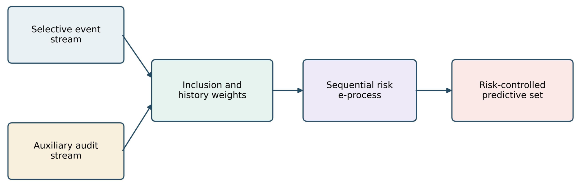
Figure 2 summarizes the information flow. The two label streams are merged only after their inclusion probabilities are computed. History weights then determine the target temporal population, and the e-process converts weighted losses into a finite-sample boundary. The output is a predictive set, not a corrected point forecast.

The architecture deliberately separates prediction, observation, and certification. The event model may be replaced without changing the risk layer. The selective stream supplies many labels near operationally important alerts, while the audit stream supplies support in silent periods. Their known propensities enter a single weighted loss. A sequential e-process then accounts for dependence through conditional expectations rather than an independence approximation. This modularity is useful in practice because model retraining, audit design, and risk-policy updates can proceed on different schedules without invalidating the logical role of each component.

Algorithm 1 summarizes the selective-observation weighted risk-control procedure used in the numerical implementation.

Algorithm 1 Selective-observation weighted risk control

Require:  Fixed grid ${\lambda }_1<\cdots <{\lambda }_J=1$, target $\alpha$, deployment buffer $\widehat{\Delta }$ (externally certified only when prospective validity is claimed), calibration confidence $\delta$, weights $a_{1:n}$, propensities $q_{1:n}$   1. Set ${\delta }_j\leftarrow \delta /J$ for $j=1,\dots ,J$   2. for  $j=1,\dots ,J$do   3.     Compute $Z_t\left({\lambda }_j\right)=I_t{L}_t\left({\lambda }_j\right)/q_t$ and ${\widehat{R}}_n\left({\lambda }_j\right)$   4.     Invert Equation (46) to obtain $U_n({\lambda }_j;{\delta }_j)$   5. end for   6. $\mathcal{F}\leftarrow \{{\lambda }_j:U_n({\lambda }_j;{\delta }_j)\le \alpha -\widehat{\Delta }\}$   7. if  $\mathcal{F}\ne ⌀$then   8.     $\widehat{\lambda }\leftarrow \min \mathcal{F}$   9. else 10.     $\widehat{\lambda }\leftarrow {\lambda }_J$ 11. end if 12. return  $C_{n+1,\widehat{\lambda }}(·)$

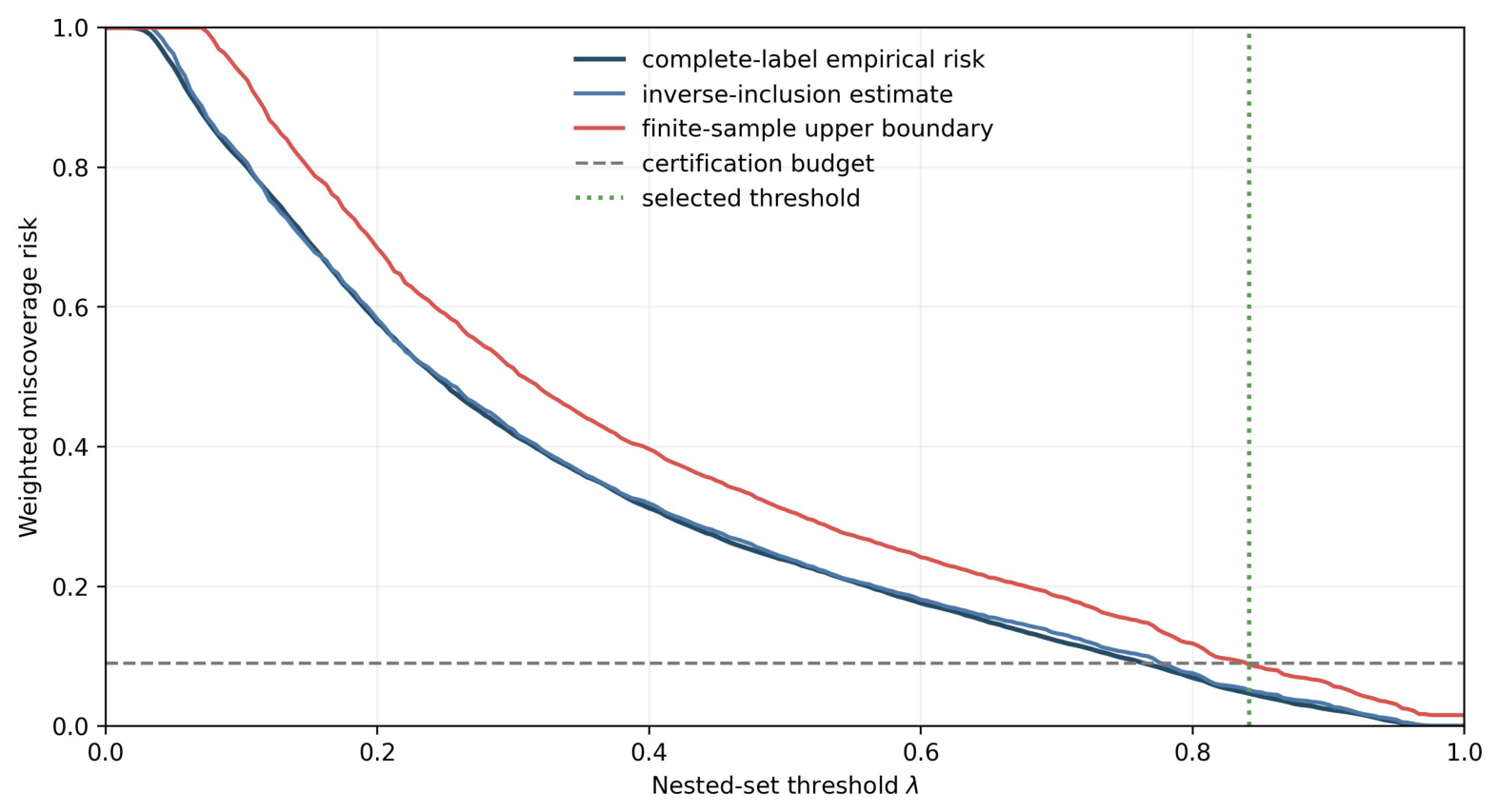
Figure 3 illustrates one calibration path. The observed weighted risk closely follows the risk computed from the hidden complete labels, while the upper boundary remains above both. The selected threshold is the first nested-set parameter for which the simultaneous boundary falls below the buffered certification budget.

The dark curve is available only to the simulator and acts as an oracle diagnostic. The inverse-inclusion estimate tracks it despite highly nonuniform label availability. The red martingale-mixture boundary adds a nonasymptotic correction that is largest for small sets, where losses and inverse-inclusion exposure are high. The green vertical line occurs where the simultaneous boundary crosses the buffered 0.09 certification budget. Its location is more conservative than the empirical crossing, which explains the moderate set-size inflation observed later. Importantly, calibration uses no hidden labels; the oracle curve is displayed solely for verification.

Remark 3.

SOWRC is conformalized risk control in the sense that it calibrates a nested family generated by any scoring model, but its proof is not an exchangeability proof. The essential mechanism is predictable inverse-inclusion weighting plus a martingale boundary. This distinction permits arbitrary temporal dependence subject to the predictability, ignorability, positivity, bounded-loss, and design-envelope conditions stated above, yet it also makes the positivity constant explicit: sparse audits widen the bound through $q_{\min }^{-1}$, exposing the price of identification rather than hiding it in an asymptotic approximation.

The replication scripts, numerical settings, and random seeds are provided in the Supplementary Materials.

For all reported calculations, the mixture contains $L=32$ equally weighted betting fractions. Let ${\eta }_{\max }$ denote the largest positive solution margin for which ${\kappa }_n\left(\eta \right)>0$. We use a geometric grid

$${\eta }_{\ell }={10}^{{log}_{10}\left({10}^{-5}\right)+\frac{\ell -1}{31}\{{log}_{10}\left(0.98{\eta }_{\max }\right)-{log}_{10}\left({10}^{-5}\right)\}},w_{\ell }=1/32,$$

(106)

for $\ell =1,\dots ,32$. Thus all 32 betting fractions and their weights are determined explicitly by Equation (106); the supplementary implementation should emit this 32-entry vector and use the same vector when reproducing the reported tables and figures. The factor $0.98$ keeps every component strictly inside the admissible region. Equation (47) is inverted by bisection on $[0,1]$ to an absolute tolerance of ${10}^{-8}$. The threshold grid is fixed before labels are inspected. These choices are numerical design decisions rather than additional stochastic assumptions.

Computational Complexity

For classification, sort the observed true-label scores once. With $n_o={\sum }_t{I}_t$, preprocessing costs

$$T_{\mathrm{sort}}=O(n_{o}log{n}_o).$$

(107)

Cumulative weighted losses over J thresholds can then be computed in

$$T_{\mathrm{grid}}=O(n_o+J).$$

(108)

Maintaining K losses and L mixture components online requires

$$T_{\mathrm{online}}=O\left(KL\right)$$

(109)

per labeled time point and memory

$$M_{\mathrm{online}}=O(KL+J).$$

(110)

The calibration layer is therefore typically cheaper than fitting the underlying event model.

Remark 4.

Efficiency is governed by two separable quantities. The predictive model controls how rapidly risk falls as the set expands, represented by the margin κ. The observation design controls the boundary through $n_{\mathrm{eff}}$. Better scores cannot repair zero support, and more audits cannot repair an uninformative score. This separation suggests a practical workflow: first guarantee positivity through randomized audits, then improve set efficiency through modeling and targeted audit allocation.

The reproducibility configuration used in Section 7 is: Python 3.13.5, NumPy 2.3.5, SciPy 1.17.0, scikit-learn 1.8.0, and statsmodels 0.14.6 for the complete-log real-data replay. For the 20-replication synthetic application studies, the stream seed is set equal to the replication index (0–19); randomized audit-mask replays use seeds 0–99. Alert and audit decisions are generated before the corresponding protected label, and the logged quantity used by SOWRC is the declared inclusion probability $q_t$, not a minimum estimated from the realized path.

7. Experiments

7.1. Design, Data, and Baselines

We evaluated SOWRC on two synthetic dependent event streams designed to isolate selective-label bias. The maintenance stream contains vibration, temperature, acoustic, load, ambient, trend, and rolling-summary variables. The financial stream contains returns, volatility, momentum, drawdown, downside variation, spread, liquidity, and a noisy observable regime proxy; the latent Markov state is never supplied to the classifier. A logistic model is fitted on the initial selectively labeled segment with inverse-inclusion weights. Calibration labels arise from either the alert rule or randomized audits, whereas the final segment is fully revealed only for evaluation. To remove the synthetic-only limitation, Section 7.4 adds a complete-log replay using a real measured weekly sensor series. There, the original outcomes are retained, selective observation is imposed prospectively from recorded history, and 100 independent audit-mask realizations quantify Monte Carlo uncertainty.

Table 4. Experimental design and representative time-series characteristics.

Characteristic	Predictive Maintenance	Financial Risk
Total time points	25,000	26,000
Feature dimension	7	8
Training/calibration/test	5500/12,000/7500	5720/12,480/7800
Default silent audit probability	0.12	0.10
Approximate alert rate	0.25	0.26
Mean event prevalence	0.25	0.14
Mean test AUC	$0.728\pm 0.014$	$0.607\pm 0.019$
Replications	20	20

summarizes the controlled benchmarks. The split proportions are 0.22, 0.48, and 0.30 for training, calibration, and testing. Moderate AUC values make set calibration nontrivial. Alert rates below one third create substantial support imbalance, while audit rates of 0.10–0.12 prevent extreme inverse weights. The financial predictor is intentionally weaker after removing the latent regime state. Thus, the comparison tests the certification layer rather than relying on an unrealistically accurate classifier. All uncertainty summaries are computed across independent time-series seeds.

The operational target is $\alpha =0.10$ with calibration confidence level $1-\delta =0.90$. For a conservative sensitivity analysis, we reserve a numerical buffer of $0.01$ and calibrate at $0.09$. This $0.01$ value is only a numerical stress buffer. It is not an estimate of ${\widehat{\Delta }}_{n,H}$ and is never used to claim Corollary 1; prospective validity requires an externally constructed certificate such as Equations (59) and (60). The deterministic grid is $\Lambda =\{0,1/240,\dots ,1\}$, and each grid point receives $\delta /241$. Baselines are alert-only calibration, unweighted observed-label calibration, a time-decayed observed-label quantile, an inverse-propensity-weighted (IPW) quantile, and an oracle quantile using complete calibration labels. Modern online, non-exchangeable, and adaptive conformal methods are not entered as nominally equivalent baselines because their published guarantees presuppose observed calibration outcomes or a support condition that the silent region violates. We therefore compare against their relevant ingredients—time adaptation and reweighting—without relabeling those implementations as methods whose assumptions are not met.

7.2. Predictive-Maintenance Results

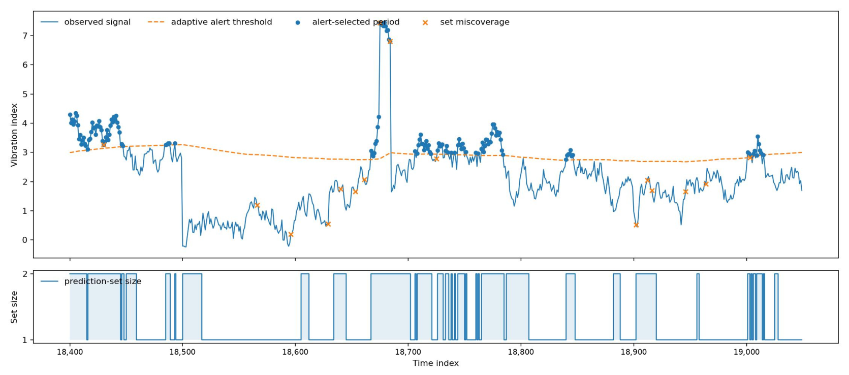
Figure 4 displays a representative deployment interval. The upper panel shows the observed signal, alert-selected periods, and realized miscoverage, while the lower panel shows prediction-set size.

Figure 4 shows abrupt transitions between calm, degrading, and fault-prone regimes. The adaptive alert threshold is now drawn explicitly; unlike the previous version, its movement is visible on the same panel as the selected periods. Near-boundary observations are therefore seen relative to the moving cutoff rather than to an implicit constant line. The plotted trajectory is illustrative rather than evidence of average performance, and we do not use an adaptive-versus-constant visual comparison as a performance claim. Typicality is assessed by the across-replication summaries in

Table 5. Predictive-maintenance performance over 20 dependent time-series replications. Entries are mean ± one standard deviation across independent trajectory seeds.

Method	Test Risk	Set Size	Silent Risk	Alert Risk
Naive-selected	$0.140\pm 0.012$	$1.180\pm 0.030$	$0.155\pm 0.013$	$0.092\pm 0.016$
Observed-unweighted	$0.129\pm 0.010$	$1.212\pm 0.033$	$0.149\pm 0.012$	$0.070\pm 0.015$
Time-decayed quantile	$0.130\pm 0.010$	$1.212\pm 0.036$	$0.149\pm 0.012$	$0.070\pm 0.016$
IPW quantile	$0.093\pm 0.012$	$1.355\pm 0.066$	$0.116\pm 0.014$	$0.023\pm 0.012$
SOWRC	$0.058\pm 0.009$	$1.537\pm 0.054$	$0.076\pm 0.011$	$0.003\pm 0.003$
Oracle-full	$0.092\pm 0.008$	$1.360\pm 0.043$	$0.116\pm 0.010$	$0.021\pm 0.009$

; no performance claim relies on this single path. The aligned lower panel confirms that SOWRC expands to the two-label set during uncertain intervals and contracts after evidence stabilizes. Most remaining errors occur in silent periods near regime changes, where alert history is sparse. The set-size path is smoother than the raw vibration signal because calibration acts on weighted cumulative losses.

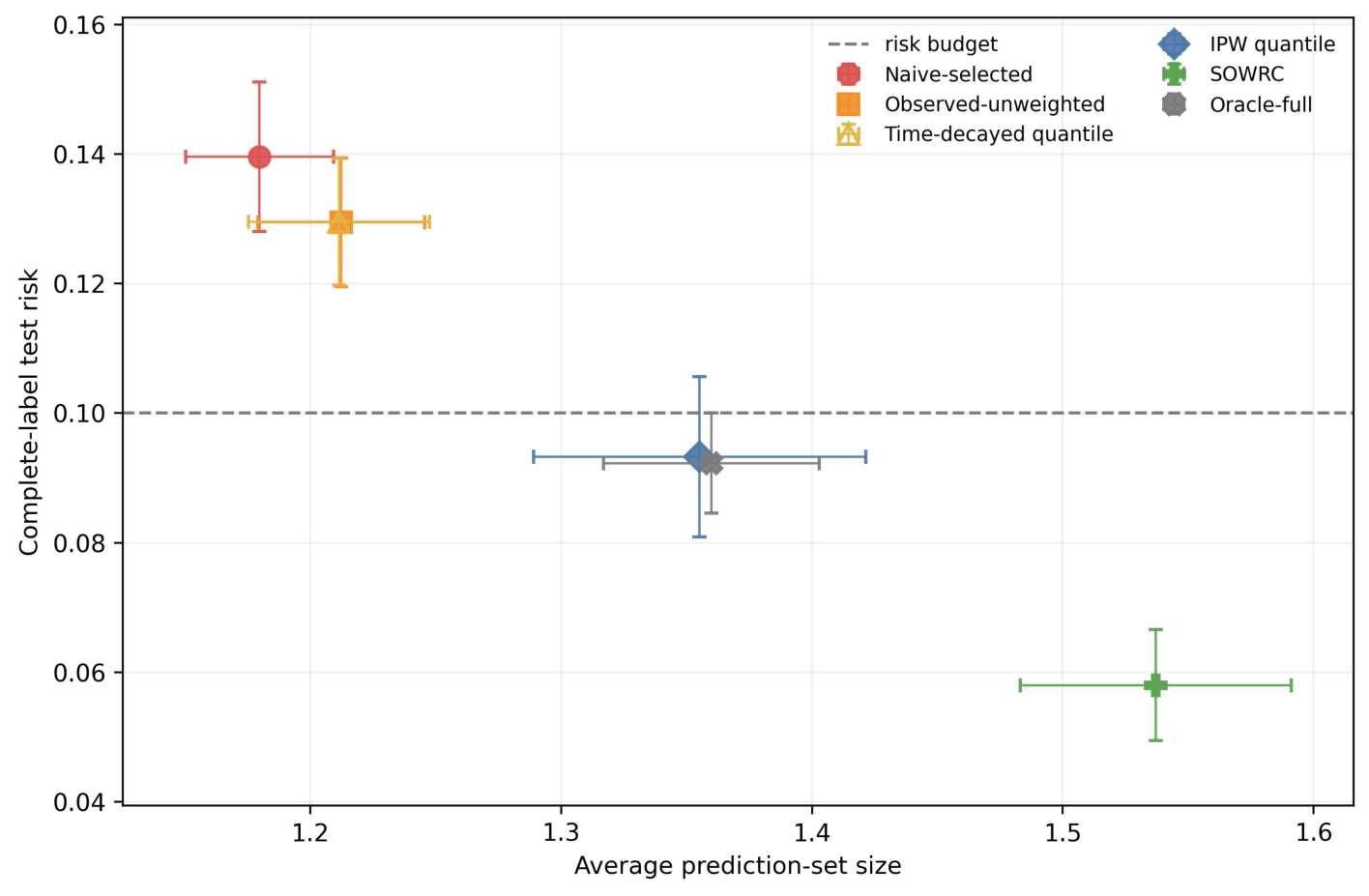
Table 5 isolates the selection effect. Alert-only calibration reaches 0.140 complete-label test risk because its apparent accuracy is concentrated in the alert region. Unweighted and time-decayed rules remain biased by the same observed-label composition. The IPW quantile corrects most of the bias but has no high-probability finite-sample certificate. SOWRC reaches 0.058 risk, with larger sets caused by the 0.01 sensitivity buffer and simultaneous grid correction. The mean calibration-to-test increase is 0.0035, but 3 of 20 seeds exceed 0.01 and the maximum increase is 0.018. Thus, these held-out results do not themselves certify Assumption 4. For the SOWRC test risk, the Monte Carlo standard error is $0.009/\sqrt{20}=0.0020$ and the normal-approximation 95% interval for the across-seed mean is approximately $[0.054,0.062]$. Reporting both the standard deviation and MCSE separates trajectory-to-trajectory variability from uncertainty in the reported mean.

Figure 5 compares complete-label test risk and average set size, with one-standard-deviation error bars. All means and bars are displayed inside the plotting window.

Figure 5 separates bias correction from statistical certification. Alert-only, unweighted, and time-decayed methods form a low-size but high-risk cluster. The IPW quantile lies close to the oracle, showing that inverse weighting removes most selection bias. SOWRC is more conservative because it also pays for simultaneous finite-sample validity and the numerical sensitivity buffer. Its entire one-standard-deviation risk bar remains below 0.10. The figure should not be read as claiming pointwise dominance: the additional set size is the explicit cost of support recovery, multiplicity control, and conservative buffering.

7.3. Financial Early-Warning Results

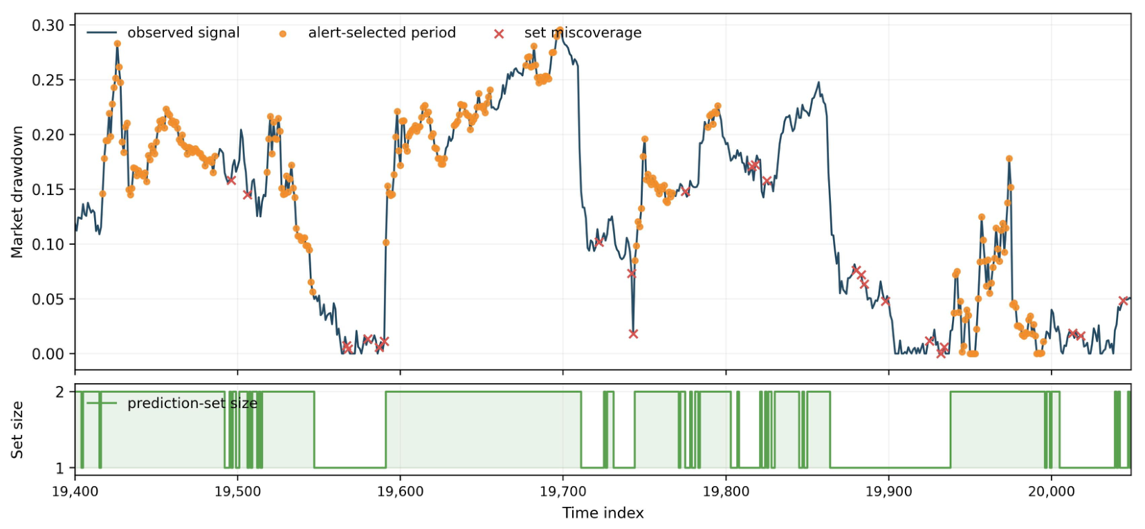
Figure 6 shows a financial deployment window with abrupt volatility and drawdown changes.

Figure 6 depicts prolonged calm periods interrupted by short stress episodes. The aligned lower panel separates discrete set expansion from the continuously scaled drawdown trajectory. The classifier observes only a noisy regime proxy, not the latent Markov state, so its discrimination is modest. SOWRC often enlarges the set before severe stress because volatility, liquidity, spread, and momentum jointly increase uncertainty. Remaining errors are dispersed across transitions rather than concentrated in one state. This behavior is consistent with aggregate population-risk control; it does not imply conditional coverage within every latent market regime, a stronger objective that would require additional structure and larger audit budgets. As with Figure 4, this trajectory is an illustrative realization rather than a hand-selected best case; the general behavior is summarized by the 20-seed statistics in

Table 6. Financial-risk performance over 20 dependent time-series replications. Entries are mean ± one standard deviation across independent trajectory seeds.

Method	Test Risk	Set Size	Silent Risk	Alert Risk
Naive-selected	$0.109\pm 0.006$	$1.083\pm 0.018$	$0.115\pm 0.006$	$0.092\pm 0.012$
Observed-unweighted	$0.108\pm 0.006$	$1.091\pm 0.020$	$0.115\pm 0.006$	$0.086\pm 0.010$
Time-decayed quantile	$0.108\pm 0.005$	$1.091\pm 0.020$	$0.115\pm 0.006$	$0.085\pm 0.013$
IPW quantile	$0.094\pm 0.009$	$1.169\pm 0.056$	$0.110\pm 0.008$	$0.047\pm 0.018$
SOWRC	$0.052\pm 0.007$	$1.524\pm 0.068$	$0.067\pm 0.008$	$0.008\pm 0.008$
Oracle-full	$0.092\pm 0.004$	$1.179\pm 0.026$	$0.111\pm 0.005$	$0.039\pm 0.011$

.

Table 6 shows a smaller but persistent selection effect in complete-label test risk. The uncorrected methods exceed the 0.10 target despite compact sets. The IPW quantile and oracle are near 0.09, whereas SOWRC reaches 0.052 because the simultaneous boundary is costly for a weaker predictor and a 0.10 audit rate. The mean calibration-to-test increase is 0.0025; 1 of 20 seeds exceeds 0.01, with a maximum increase of 0.0118. The result demonstrates conservative held-out performance, not unconditional future validity or an empirical proof of the drift certificate. For SOWRC, the test-risk MCSE is $0.007/\sqrt{20}=0.0016$, giving an approximate 95% interval of $[0.049,0.055]$ for the across-seed mean.

7.4. Complete-Log Real-Data Replay and Conservativeness

To complement the controlled synthetic experiments, we added a complete-log replay based on the weekly Mauna Loa atmospheric CO₂ series distributed with statsmodels [33]. The purpose is not to claim a domain-specific CO₂ forecasting contribution, but to test selective observation on a genuine dependent sensor record for which every outcome is available before masking. The 59 missing weekly measurements in the distributed series are filled by one-sided forward filling before lagged features are constructed, so no future event label is used in preprocessing. After removing unavailable lags, 2231 weekly observations remain. We use 557 observations for model fitting, 1003 for calibration, and 671 for complete-label testing. An event is defined as an absolute next-week CO₂ change exceeding the 80th percentile of the training changes. A logistic score uses lagged level/change, rolling mean and scale, and seasonal terms. The alert threshold is fixed at the 75th percentile of training scores, producing a calibration alert rate of 0.290. Silent labels are then independently audited with probability $\rho =0.30$. The threshold grid has 121 deterministic values, and each selective-observation method is replayed under 100 independently generated audit masks (seeds 0–99).

Table 7. Complete-log CO₂ replay under selective observation. Entries are mean ± standard deviation over 100 independent audit masks; “Oracle-full” uses all calibration labels before masking. The reported variability is conditional on this single observed CO₂ time series and reflects only repeated audit-mask randomization; it does not quantify uncertainty across alternative real-world time series or uncertainty from selecting this particular series.

Method	Complete-Label Test Risk	Mean Set Size
Alert-only	$0.0402\pm 0.0000$	$1.8197\pm 0.0000$
Observed-unweighted	$0.0760\pm 0.0052$	$1.7459\pm 0.0091$
IPW quantile	$0.1076\pm 0.0070$	$1.6629\pm 0.0186$
SOWRC	$0.0185\pm 0.0023$	$1.9018\pm 0.0136$
Oracle-full	$0.1103\pm 0.0000$	$1.6587\pm 0.0000$

shows the cost of finite-sample certification on a non-synthetic trajectory. SOWRC is markedly conservative, whereas the oracle and IPW quantile are much closer to the 0.10 target. For SOWRC the MCSE of mean test risk is $0.0023/\sqrt{100}=0.00023$, yielding an approximate 95% Monte Carlo interval $[0.0181,0.0190]$. Because the complete labels are retained only for evaluation, this replay also makes clear which quantities are deployment diagnostics rather than inputs to the certificate. These Monte Carlo intervals should therefore be interpreted as conditional audit-mask variability for one fixed trajectory, not as a population-level interval over possible sensor series.

Table 8. Conservativeness decomposition on the complete-log replay ($\rho =0.30$, 100 audit masks). The pointwise martingale row is a diagnostic without grid-selection validity; Bonferroni restores simultaneous protection for the threshold sweep.

Calibration Rule	Test Risk	Mean Set Size
IPW empirical risk only	$0.1076\pm 0.0070$	$1.6629\pm 0.0186$
Martingale, pointwise $\delta =0.10$	$0.0370\pm 0.0094$	$1.8298\pm 0.0207$
Martingale + Bonferroni grid	$0.0185\pm 0.0023$	$1.9018\pm 0.0136$
Grid + numerical 0.01 buffer	$0.0145\pm 0.0014$	$1.9214\pm 0.0077$

separates four sources that were previously bundled together. Inverse weighting mainly repairs selective-observation bias; the martingale deviation term causes the largest enlargement; simultaneous Bonferroni protection adds a further visible cost; and the 0.01 numerical buffer is comparatively smaller. This decomposition does not imply that the pointwise row is a valid replacement for the simultaneous procedure: it is included only to quantify the multiplicity price. Sharper simultaneous boundaries that exploit monotonicity across $\lambda$ are an important direction for reducing this price.

The misspecification experiment in

Table 9. Propensity-misspecification diagnostic for the complete-log replay. The logged inclusion probability used by SOWRC is multiplied by the indicated factor before clipping; values are mean ± standard deviation over 100 audit masks.

Propensity Scale	Test Risk	Mean Set Size
0.8	$0.0110\pm 0.0040$	$1.9390\pm 0.0199$
0.9	$0.0159\pm 0.0011$	$1.9173\pm 0.0058$
1.0	$0.0185\pm 0.0023$	$1.9018\pm 0.0136$
1.1	$0.0205\pm 0.0025$	$1.8904\pm 0.0128$
1.2	$0.0227\pm 0.0030$	$1.8791\pm 0.0134$

is deliberately reported as a sensitivity diagnostic rather than a validity theorem. Underestimating inclusion probabilities increases the inverse weights and therefore enlarges the sets; overestimation has the opposite effect. Formal validity with estimated propensities still requires the multiplicative calibration envelope stated in Proposition 1. In practice, this envelope can be assessed from randomized logging records, held-out propensity calibration, or cross-fitted policy models before outcomes from the calibrated decision are used.

7.5. Audit Ablation and Selection-Level Certificate Validation

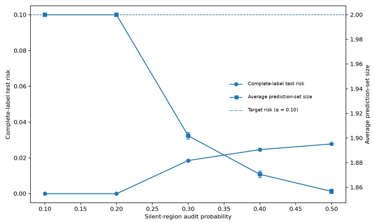
The complete-log replay also permits the audit rate itself to be varied without changing the underlying trajectory or predictor. We use $\rho \in \{0.10,0.20,0.30,0.40,0.50\}$ and 100 independent audit masks at every setting. Error bars in Figure 7 are 95% Monte Carlo intervals for the across-mask means.

At $\rho =0.10$ and $0.20$, the simultaneous boundary is so wide that the safe terminal action is selected in all masks, giving the full two-label set and zero empirical test loss. At $\rho =0.30$, the mean test risk is $0.0185\pm 0.0023$; increasing the audit rate to 0.40 and 0.50 raises mean risk to approximately 0.0247 and 0.0278 while reducing set size, because the effective sample size grows and the certificate becomes less conservative. This behavior is the empirical counterpart of Equation (82): the audit floor controls both identifiability and the statistical price of inverse weighting.

We also replaced the earlier fixed-threshold diagnostic by a selection-level experiment that runs the final threshold-selection rule on a persistent two-state Markov score process. Conditional losses are generated from state-dependent beta distributions, the candidate grid contains $J=41$ fixed thresholds, and the true selected conditional population risk is available analytically for checking. For each of the eight configurations below, 500 independent trajectories are generated. We vary horizon, audit rate, confidence level, target risk, and state persistence. A failure occurs when the risk of the threshold actually selected by SOWRC exceeds the declared target after the certificate is applied.

Table 10. Selection-level finite-sample validation over 500 independent dependent-process replications per configuration. “Fallback” is the fraction of runs selecting the safe terminal action. This experiment is intended to confirm implementation correctness and conservativeness, not tight calibration to the nominal $\delta$.

n	$\mathit{\rho }$	$\mathit{\delta }$	$\mathit{\alpha }$	Persistence	Failures/500	95% Upper	Fallback
1000	0.10	0.10	0.10	0.95	0	0.006	1.000
3000	0.10	0.10	0.10	0.95	0	0.006	0.000
3000	0.05	0.10	0.10	0.95	0	0.006	1.000
3000	0.20	0.10	0.10	0.95	0	0.006	0.000
3000	0.10	0.05	0.10	0.95	0	0.006	0.000
3000	0.10	0.20	0.10	0.95	0	0.006	0.000
3000	0.10	0.10	0.05	0.95	0	0.006	1.000
3000	0.10	0.10	0.10	0.80	0	0.006	0.000

reports the resulting selection-level finite-sample validation results.

Across all $8\times 500=4000$ selection-level replications, no failure was observed. With zero failures in 500 trials, the one-sided exact 95% binomial upper bound is 0.006 for each configuration. The result should not be read as evidence that the procedure is calibrated tightly to the nominal $\delta$: the fallback rates and positive certificate gaps show substantial conservatism, especially for short horizons, sparse audits, or the smaller target risk. Its purpose is instead to verify that the data-dependent grid selection—the central operation of SOWRC—does not invalidate the finite-sample protection in these dependent simulations.

7.6. Implementation Checks and Limitations

All experiments use exact logged inclusion probabilities and a deterministic lower propensity bound supplied by the audit design; the code never substitutes a favorable minimum computed from the realized path. The candidate grid is fixed before labels are inspected, eliminating data reuse from empirical score quantiles. Predictable weights increase linearly from 0.95 to 1.05, and the mixture uses 32 admissible betting fractions. The implementation searches all 241 thresholds with Bonferroni confidence allocation. The code exports every replication, drift diagnostic, representative stream, summary table, validation experiment, and figure. The two application streams remain synthetic controlled demonstrations, but the complete-log CO₂ replay now adds a real dependent sensor record with selective labels imposed only after the fact. The replay is intentionally a methodological stress test rather than a claim of domain-specific superiority; complete labels are used solely for post hoc evaluation.

Three limitations remain. First, conditional ignorability can fail when annotators use latent information absent from the recorded history. Randomized audits are preferable in that setting. Second, future-horizon control is not distribution-free under unrestricted drift; it requires an external certificate satisfying Assumption 4, with its error ${\delta }_{\mathrm{dep}}$ included, or continued online auditing through Theorem 3. Third, the guarantee is weighted population-level risk, not equal conditional risk in every regime or subgroup. These distinctions prevent calibration-population validity, prospective transfer, and conditional coverage from being conflated.

Remark 5.

The revised experiments distinguish three questions. Inverse weighting addresses bias from selective observation. The martingale boundary certifies the weighted calibration population. A separately certified drift envelope is required to connect that certificate to a future deployment horizon; the numerical buffer used here is only a sensitivity choice. None of these steps substitutes for another. This separation makes the source of conservatism visible and prevents low selected-sample error from being mistaken for future population-risk control.

8. Conclusions and Future Work

This paper studied predictive sets when labels are observed selectively along a dependent stochastic process. Population risk is non-identifiable on any region with zero labeling probability. A randomized audit stream restores support, and SOWRC combines alert and audit labels through predictable inverse-inclusion losses. A martingale-mixture boundary then provides finite-sample control of the weighted calibration population on a deterministic threshold grid. The prospective result states the additional condition required for future use: an externally certified deployment-drift envelope, explicit error allocation, and a matching calibration buffer.

The theory now separates four logically distinct components. Positivity determines identification. Effective sample size determines statistical precision. Monotone nested losses and a safe terminal action justify data-dependent threshold selection. A deployment envelope determines whether a calibration certificate transfers to future events. The experiments use a deterministic grid, remove latent-state leakage, and name baselines according to their implementations. They now also include a complete-log real-data replay with 100 audit masks and Monte Carlo uncertainty, a decomposition of the main sources of conservativeness, a propensity-misspecification sensitivity analysis, and selection-level validation over 4000 dependent-process replications.

Three directions merit further study. First, audit policies should be optimized jointly with prediction under a long-run labeling budget while preserving minimum support. Second, deployment-drift envelopes should be learned from independent auxiliary trajectories with simultaneous uncertainty quantification. Third, doubly robust and distributionally robust extensions should control delayed outcomes, partially observed covariates, and regime-specific risks without sacrificing anytime validity.

References

1. Angelopoulos, A.N.; Bates, S.; Fisch, A.; Lei, L.; Schuster, T. Conformal risk control. In Proceedings of the Twelfth International Conference on Learning Representations, Vienna, Austria, 7–11 May 2024; OpenReview: Amherst, MA, USA, 2024. [Google Scholar]
2. Doria, S. Bayesian updating for stochastic processes in infinite-dimensional normed vector spaces. Axioms 2025, 14, 927. [Google Scholar] [CrossRef] [Scilit]
3. Bao, Y.; Huo, Y.; Ren, H.; Zou, C. CAP: A general algorithm for online selective conformal prediction with FCR control. J. Mach. Learn. Res. 2025, 26, 1–74. [Google Scholar]
4. Gibbs, I.; Candès, E.J. Conformal inference for online prediction with arbitrary distribution shifts. J. Mach. Learn. Res. 2024, 25, 1–36. [Google Scholar]
5. Xu, C.; Jiang, H.; Xie, Y. Conformal prediction for multi-dimensional time series by ellipsoidal sets. In Proceedings of the 41st International Conference on Machine Learning; PMLR: Cambridge, MA, USA, 2024; Volume 235, pp. 55076–55099. [Google Scholar]
6. Strang, A. A theoretical review of area production rates as test statistics for detecting nonequilibrium dynamics in Ornstein–Uhlenbeck processes. Axioms 2024, 13, 820. [Google Scholar] [CrossRef] [Scilit]
7. Oliveira, R.I.; Orenstein, P.; Ramos, T.; Romano, J.V. Split conformal prediction and non-exchangeable data. J. Mach. Learn. Res. 2024, 25, 1–38. [Google Scholar]
8. Zheng, F.; Proutière, A. Conformal predictions under Markovian data. In Proceedings of the 41st International Conference on Machine Learning; PMLR: Cambridge, MA, USA, 2024; Volume 235, pp. 61470–61497. [Google Scholar]
9. Galvão Lopes, A.; Goubault, E.; Putot, S.; Pautet, L. ConForME: Multi-horizon conditional conformal time series forecasting. In Proceedings of the Thirteenth Symposium on Conformal and Probabilistic Prediction with Applications; PMLR: Cambridge, MA, USA, 2024; Volume 230, pp. 345–365. [Google Scholar]
10. Jacquet, O.; Oscar, W.; Vaillant, J. Partially observed two-phase point processes. Axioms 2026, 15, 59. [Google Scholar] [CrossRef] [Scilit]
11. Zhou, Y.; Lindemann, L.; Sesia, M. Conformalized adaptive forecasting of heterogeneous trajectories. In Proceedings of the 41st International Conference on Machine Learning; PMLR: Cambridge, MA, USA, 2024; Volume 235, pp. 62002–62056. [Google Scholar]
12. Prinzhorn, D.; Nijdam, T.; van der Linden, P.; Timans, A. Conformal time series decomposition with component-wise exchangeability. In Proceedings of the Thirteenth Symposium on Conformal and Probabilistic Prediction with Applications; PMLR: Cambridge, MA, USA, 2024; Volume 230, pp. 432–465. [Google Scholar]
13. Hallberg Szabadváry, J. Adaptive conformal inference for multi-step ahead time-series forecasting online. In Proceedings of the Thirteenth Symposium on Conformal and Probabilistic Prediction with Applications; PMLR: Cambridge, MA, USA, 2024; Volume 230, pp. 250–263. [Google Scholar]
14. Zhang, H.; Sun, J.; Wen, X. Stationary distribution and density function for a high-dimensional stochastic SIS epidemic model with mean-reverting stochastic process. Axioms 2024, 13, 768. [Google Scholar] [CrossRef] [Scilit]
15. Blot, V.; Angelopoulos, A.N.; Jordan, M.I.; Brunel, N.J.-B. Automatically adaptive conformal risk control. In Proceedings of the 28th International Conference on Artificial Intelligence and Statistics; PMLR: Cambridge, MA, USA, 2025; Volume 258, pp. 19–27. [Google Scholar]
16. Einbinder, B.-S.; Feldman, S.; Bates, S.; Angelopoulos, A.N.; Gendler, A.; Romano, Y. Label noise robustness of conformal prediction. J. Mach. Learn. Res. 2024, 25, 1–66. [Google Scholar]
17. Gnecco, N.; Peters, J.; Engelke, S.; Pfister, N. Boosted control functions: Distribution generalization and invariance in confounded models. J. Mach. Learn. Res. 2026, 27, 1–57. [Google Scholar]
18. Howard, S.R.; Ramdas, A.; McAuliffe, J.; Sekhon, J. Time-uniform, nonparametric, nonasymptotic confidence sequences. Ann. Stat. 2021, 49, 1055–1080. [Google Scholar] [CrossRef] [Scilit]
19. Vovk, V.; Wang, R. E-values: Calibration, combination, and applications. Ann. Stat. 2021, 49, 1736–1754. [Google Scholar] [CrossRef] [Scilit]
20. Jonkers, J.; Van Wallendael, G.; Duchateau, L.; Van Hoecke, S. Conformal predictive systems under covariate shift. In Proceedings of the Thirteenth Symposium on Conformal and Probabilistic Prediction with Applications; PMLR: Cambridge, MA, USA, 2024; Volume 230, pp. 406–423. [Google Scholar]
21. Hussain, T.; Villamor, E.; Shakil, M.; Ahsanullah, M.; Kibria, B.M.G. A novel probabilistic model for streamflow analysis and its role in risk management and environmental sustainability. Axioms 2026, 15, 113. [Google Scholar] [CrossRef] [Scilit]
22. Chvoinikov, D.; Novikov, S.; Šiaulys, J. Extremes of product of Gaussian random variables. Axioms 2026, 15, 425. [Google Scholar] [CrossRef] [Scilit]
23. Hulsman, R.; Comte, V.; Bertolini, L.; Wiesenthal, T.; Puertas Gallardo, A.; Ceresa, M. Conformal risk control for pulmonary nodule detection. In Proceedings of the Fourteenth Symposium on Conformal and Probabilistic Prediction with Applications; PMLR: Cambridge, MA, USA, 2025; Volume 266, pp. 445–463. [Google Scholar]
24. Zhang, C.; Li, T.; Xie, J.; Kong, L.; Jiang, B. Transfer conformal predictive inference for regression. J. Mach. Learn. Res. 2026, 27, 1–68. [Google Scholar]
25. Barber, R.F.; Candès, E.J.; Ramdas, A.; Tibshirani, R.J. Conformal prediction beyond exchangeability. Ann. Stat. 2023, 51, 816–845. [Google Scholar] [CrossRef] [Scilit]
26. Zaffran, M.; Féron, O.; Goude, Y.; Josse, J.; Dieuleveut, A. Adaptive conformal predictions for time series. In Proceedings of the 39th International Conference on Machine Learning; PMLR: Cambridge, MA, USA, 2022; Volume 162, pp. 25834–25866. [Google Scholar]
27. Barber, R.F.; Pananjady, A. Predictive inference for time series: Why is split conformal effective despite temporal dependence? In Proceedings of the 37th International Conference on Algorithmic Learning Theory; PMLR: Cambridge, MA, USA, 2026; Volume 313, pp. 1–24. [Google Scholar]
28. Chen, B.; Zhou, X.; Cheng, L. Post-training adaptive conformal prediction for incomplete time series. Trans. Mach. Learn. Res. 2026. Available online: https://openreview.net/forum?id=KMBU4wx79B (accessed on 19 September 2026).
29. Bates, S.; Angelopoulos, A.N.; Lei, L.; Malik, J.; Jordan, M.I. Distribution-free, risk-controlling prediction sets. J. ACM 2021, 68, 43. [Google Scholar] [CrossRef] [Scilit]
30. Angelopoulos, A.N.; Bates, S. Conformal prediction: A gentle introduction. Found. Trends Mach. Learn. 2023, 16, 494–591. [Google Scholar] [CrossRef] [Scilit]
31. Horvitz, D.G.; Thompson, D.J. A generalization of sampling without replacement from a finite universe. J. Am. Stat. Assoc. 1952, 47, 663–685. [Google Scholar] [CrossRef]
32. Robins, J.M.; Rotnitzky, A.; Zhao, L.P. Estimation of regression coefficients when some regressors are not always observed. J. Am. Stat. Assoc. 1994, 89, 846–866. [Google Scholar] [CrossRef]
33. Seabold, S.; Perktold, J. Statsmodels: Econometric and statistical modeling with Python. In Proceedings of the 9th Python in Science Conference, Austin, TX, USA, 28 June–3 July 2010; SciPy: Austin, TX, USA, 2010; pp. 92–96. [Google Scholar]
Figure 1. Selective labels and silent-region audits under a visibly history-adaptive alert threshold. The threshold is updated from lagged observed scores only, so the change in the selection pattern is predictable rather than label-driven.
Axioms 15 00706 g001
Figure 2. SOWRC information flow from selective labels and audits to risk-controlled predictive sets.
Axioms 15 00706 g002
Figure 3. Weighted risk estimate and finite-sample boundary across nested-set thresholds.
Axioms 15 00706 g003
Figure 4. Maintenance signal, adaptive alert threshold, alert-selected periods, set size, and SOWRC miscoverage over time.
Axioms 15 00706 g004
Figure 5. Test-risk–set-size trade-off with one-standard-deviation error bars.
Axioms 15 00706 g005
Figure 6. Financial drawdown, alert periods, set size, and SOWRC miscoverage over time.
Axioms 15 00706 g006
Figure 7. Complete-log SOWRC replay as the silent-region audit probability varies. Points are means over 100 audit masks; bars are 95% Monte Carlo intervals. The bars quantify audit-mask variability conditional on the single replayed time series and do not include across-series or series-selection uncertainty.
Axioms 15 00706 g007