Local Convergence of the Gauss–Newton–Broyden Method for Solving Nonlinear Least Squares Problems

Abstract

The Gauss–Newton–Broyden method is proposed and investigated for solving a nonlinear least squares problem with operator decomposition. This method is obtained from the Gauss–Newton method by replacing the Jacobian matrix of a nonlinear operator with the sum of the derivative of the differentiable part of the operator and the matrix computed by the Broyden update formula for the other part of the nonlinear vector function. A local convergence theorem for the proposed method, under the classical Lipschitz conditions and for problems with zero residual, is proved. The results of numerical experiments are also presented.

1. Introduction

Let us consider the nonlinear least squares problem (NLSP) [1,2,3,4]. It is necessary to find ${\kappa }^{*}\in D$ such that

$$h\left({\kappa }^{*}\right)=\underset{x\in D}{\min }h\left(x\right),h\left(x\right)={\displaystyle \frac{1}{2}}\mathcal{H}{\left(x\right)}^{\top }\mathcal{H}\left(x\right).$$

(1)

Here, $\mathcal{H}:D\subseteq \mathrm{I}{\mathrm{R}}^{\mathrm{n}}\to \mathrm{I}{\mathrm{R}}^{\mathrm{m}}$ is a vector-valued function that is nonlinear in the variable x and $m\ge n$. Problem (1) is said to have zero residual if $h\left({\kappa }^{*}\right)=0$, and nonzero residual otherwise. The problem (1) with zero residual and $m=n$ can be viewed as a system of nonlinear algebraic or transcendental equations.

Nonlinear least squares problems arise in a wide range of scientific and engineering applications, including the solution of overdetermined systems of equations, parameter estimation for physical processes based on measurement data, construction of nonlinear regression models, parameter estimation and hypothesis testing in mathematical statistics, control of various objects and processes [5,6], and the solution of nonlinear complementarity problems [7,8,9].

The basic numerical methods for solving problem (1) are the Gauss–Newton method

$$x_{k+1}=x_k-{\left[{\mathcal{H}}^{\prime }{\left(x_k\right)}^{\top }{\mathcal{H}}^{\prime }\left(x_k\right)\right]}^{-1}{\mathcal{H}}^{\prime }{\left(x_k\right)}^{\top }\mathcal{H}\left(x_k\right),k\ge 0,$$

(2)

and Levenberg–Marquardt method

$$x_{k+1}=x_k-{[{\mathcal{H}}^{\prime }{\left(x_k\right)}^{\top }{\mathcal{H}}^{\prime }\left(x_k\right)+\lambda I]}^{-1}{\mathcal{H}}^{\prime }{\left(x_k\right)}^{\top }\mathcal{H}\left(x_k\right),k\ge 0.$$

(3)

Methods (2) and (3) have the convergence order equal to 2 in the case of zero residual [10,11,12]. But, these iterative methods require the evaluation of derivatives, which can be computationally expensive. That is why there are many studies that try to eliminate this drawback. One of them is the construction of multi-step methods in which the matrix of derivatives is calculated once for several steps. In [2,13], the authors investigated the two-step Gauss–Newton Werner-type method under generalized Lipschitz conditions.

In practice, however, many problems involve functions whose values are obtained from experimental data, so analytical derivatives may not be available. Moreover, when functions are defined by complicated analytical expressions, computing their partial derivatives can be expensive. Therefore, derivative-free methods are particularly attractive in such situations. The derivative-free methods use a finite difference approximation of the Jacobian matrix [3,4,14] or a matrix of divided differences computed similar to one in [15]. The divided difference of the function H at the points x and y is denoted by $\mathcal{H}(x,y)$. Elements of this matrix are computed using the following formula:

$$\mathcal{H}{(x,y)}_{i,j}={\displaystyle \frac{{\mathcal{H}}_i\left(\zeta \right)-{\mathcal{H}}_i\left(\theta \right)}{x_j-y_j}},i=1,\dots ,m,j=1,\dots ,n.$$

(4)

Here, $\zeta ={(x_1,\dots ,x_j,y_{j+1},\dots ,y_n)}^{\top }$ and $\theta ={(x_1,\dots ,x_{j-1},y_j,\dots ,y_n)}^{\top }$, x and y are distinct points in $\mathrm{I}{\mathrm{R}}^{\mathrm{n}}$. In particular, methods with divided differences include the Secant-type method

$$\begin{array}{cc}\hfill A_k& =\mathcal{H}(x_k,x_{k-1}),\hfill \\ \hfill x_{k+1}& =x_k-{\left[A_k^{\top }{A}_k\right]}^{-1}{A}_k^{\top }\mathcal{H}\left(x_k\right),k\ge 0,\hfill \end{array}$$

the Potra-type method with $A_k=\mathcal{H}(x_k,x_{k-1})+\mathcal{H}(x_{k-2},x_k)-\mathcal{H}(x_{k-2},x_{k-1})$ or the Kurchatov-type method with $A_k=\mathcal{H}(2x_k-x_{k-1},x_{k-1})$. Convergence analysis of these methods under classical Lipschitz conditions has been conducted in [5,16], estimates of method errors have been obtained, and it has been established that the convergence orders of these methods in the case of zero residual are equal to ${\displaystyle \frac{1+\sqrt{5}}{2}}$, $1.839\dots$ and 2, respectively.

In [3,17], the authors considered a modification of the Levenberg–Marquardt method (3) with approximation of ${\mathcal{H}}^{\prime }\left(x_k\right)$ based on Broyden’s update formula. In [17], a numerical study of the method was carried out, and its effectiveness for solving inverse problems of very complex physical models was shown. The convergence study of the Broyden method and its modification for systems of nonlinear equations can be found in [1,18,19].

Several authors have investigated NLSP in which the nonlinear vector function is represented as the sum of two components [20,21,22]:

$$\mathcal{H}\left(x\right)\equiv \mathcal{F}\left(x\right)+\mathcal{G}\left(x\right),$$

where $\mathcal{F}$ and $\mathcal{G}:D\subseteq \mathrm{I}{\mathrm{R}}^{\mathrm{n}}\to \mathrm{I}{\mathrm{R}}^{\mathrm{m}}$. The goal is to find ${\kappa }^{*}\in D$ such that

$$h\left({\kappa }^{*}\right)=\underset{x\in D}{\min }h\left(x\right),h\left(x\right)={\displaystyle \frac{1}{2}}{(\mathcal{F}\left(x\right)+\mathcal{G}\left(x\right))}^{\top }(\mathcal{F}\left(x\right)+\mathcal{G}\left(x\right)).$$

(5)

It is known that $\mathcal{F}$ is a differentiable function, whereas $\mathcal{G}$ is continuous and can be either unavailable analytically or represented by a complicated analytical expression or nondifferentiable on D. That is, $\mathcal{G}$ can be either differentiable or nondifferentiable.

For the numerical solution of problems of this type, differential-difference methods are often used. They use the sum of the Jacobian matrix of the differentiable part F and the divided difference of G instead of the full Jacobian matrix. The most well-known methods for this type of problem are the Gauss–Newton–Secant method [20]

$$\begin{array}{cc}\hfill A_k& ={\mathcal{F}}^{\prime }\left(x_k\right)+\mathcal{G}(x_k,x_{k-1}),\hfill \\ \hfill x_{k+1}& =x_k-{\left[A_k^{\top }{A}_k\right]}^{-1}{A}_k^{\top }\mathcal{H}\left(x_k\right),k\ge 0,\hfill \end{array}$$

(6)

the Gauss–Newton–Potra method [21] and the Gauss–Newton–Kurchatov method [22]. The local convergence of the Gauss–Newton–Secant and Gauss–Newton–Potra methods is investigated under classical Lipschitz conditions, and the Gauss–Newton–Kurchatov method under generalized conditions. Error estimates of the methods are obtained, and, for problems with zero residual, it is shown that their convergence orders coincide with those of the corresponding difference methods. Note that a similar approach has proven itself well for solving nonlinear equations with operator decomposition [23,24]. The computational complexity of one iteration of these methods is also somewhat different. The main difference lies in the computation of the divided differences. From Formula (4), the Secant-type method requires the evaluation of $m(n+1)$ scalar functions of n variables and $3mn$ arithmetic operations, the  Potra-type method requires the evaluation of $3mn$ functions and $11mn$ arithmetic operations, and the Kurchatov-type method requires the evaluation of $m(n+1)$ functions and $3mn+2n$ arithmetic operations. Taking into account that $\mathcal{G}\left(x_{k-2}\right)$, $\mathcal{G}\left(x_{k-1}\right)$, $\mathcal{G}\left(x_k\right)$ and corrections are computed at the current and previous iterations, we can see that these estimates of the computational complexity can be slightly relaxed.

We introduce the Gauss–Newton–Broyden method for solving the NLSP (5)

$$\begin{array}{cc}\hfill A_k& ={\mathcal{F}}^{\prime }\left(x_k\right)+B_k,\hfill \\ \hfill x_{k+1}& =x_k-{\left[A_k^{\top }{A}_k\right]}^{-1}{A}_k^{\top }\mathcal{H}\left(x_k\right),k\ge 0,\hfill \end{array}$$

(7)

where

$$\begin{array}{c}{B}_{k+1}=B_k+{\displaystyle \frac{(y_k-B_k{s}_k)s_k^{\top }}{s_k^{\top }{s}_k}},\hfill \\ s_k=x_{k+1}-x_k,y_k=\mathcal{G}\left(x_{k+1}\right)-\mathcal{G}\left(x_k\right).\hfill \end{array}$$

(8)

Here, $B_0$ is a given matrix. To form the matrix $B_k$, it is necessary to evaluate $2m$ scalar functions of n variables, compute the difference of two pairs of vectors of dimensions m and n, calculate the scalar product of two vectors of dimension n, multiply an $m\times n$ matrix by an n-dimensional column vector, compute the difference of two m-dimensional vectors, compute the outer product of an m-dimensional column vector and an n-dimensional row vector, divide an $m\times n$ matrix by a scalar, and add two $m\times n$ matrices. Thus, the computational complexity of forming a matrix $B_k$ is $5mn+3n+m-1$ arithmetic operations and the evaluation of $2m$ scalar functions of n variables. Taking into account that some calculations are performed on the current and previous iterations, these estimates of the computational complexity can also be reduced. Therefore, for functions with a complex analytical form, the computational cost of one iteration of the Gauss–Newton–Broyden method (7) is expected to be lower than that of the Gauss–Newton–Secant method (6).

Also, a feature of the proposed method (7) is that a partial, rather than a full, approximation of the Jacobian matrix is used. In Broyden-type methods, $B_k\approx {\mathcal{H}}^{\prime }\left(x_k\right)$ [3,17]. Since the full calculation of ${\mathcal{H}}^{\prime }\left(x\right)$ can be computationally expensive (or impossible), this approach can be considered as a trade-off between the computation cost of the derivative and the accuracy of the Jacobian matrix approximation. We also conduct the convergence study of the Gauss–Newton–Broyden method (7) under classical Lipschitz conditions. A number of numerical experiments have been conducted to demonstrate the applicability and effectiveness of this approach.

2. Local Convergence Analysis

We establish the local convergence of the Gauss–Newton–Broyden method (7) under classical Lipschitz conditions. The convergence study was conducted in the case of problems (5) with zero residual, i.e., $\parallel \mathcal{H}\left({\kappa }^{*}\right)\parallel =0$.

Let I denote the identity matrix and $A_{*}={\mathcal{H}}^{\prime }\left({\kappa }^{*}\right)$. Throughout the theoretical analysis, the Euclidean vector norm and the corresponding matrix norm are used. For Euclidean norm $\parallel A\parallel =\parallel A^{\top }\parallel$, where A is some matrix.

We first present several auxiliary lemmas needed to establish the main result.

Lemma 1

([18,19]). Let $s\in \mathrm{I}{\mathrm{R}}^{\mathrm{n}}$, $n\ge 2$ and $s^{\top }s=1$. Then,

$$\parallel I-s{s}^{\top }\parallel =1.$$

Lemma 2.

Let ${\kappa }^{*}\in D$ be a solution of the problem (5) and $D\subseteq \mathrm{I}{\mathrm{R}}^{\mathrm{n}}$ be an open convex domain, $\left\{x_k\right\}\subset D$, and $x_k\ne {\kappa }^{*}$. Let $\mathcal{F},\mathcal{G}:D\to \mathrm{I}{\mathrm{R}}^{\mathrm{m}}$, $\mathcal{F}\in C^1\left(D\right)$, $\mathcal{G}$ is differentiable at the point ${\kappa }^{*}$, and suppose that the following conditions hold:

$$\parallel {\mathcal{F}}^{\prime }\left(x\right)-{\mathcal{F}}^{\prime }\left(y\right)\parallel \le L\parallel x-y\parallel ,x,y\in D,$$

(9)

$$\parallel \mathcal{G}(x,y)-{\mathcal{G}}^{\prime }\left({\kappa }^{*}\right)\parallel \le M\left(\parallel x-{\kappa }^{*}\parallel +\parallel y-{\kappa }^{*}\parallel \right),x,y\in D.$$

(10)

Let $B_{k+1}$ be defined by Formula (8) and $A_{k+1}={\mathcal{F}}^{\prime }\left(x_{k+1}\right)+B_{k+1}$. Then, for all $k\ge 0$, the following estimates hold:

$$\parallel A_{k+1}-A_{*}\parallel \le \parallel B_k-{\mathcal{G}}^{\prime }\left({\kappa }^{*}\right)\parallel +L\parallel x_{k+1}-{\kappa }^{*}\parallel +M\left(\parallel x_{k+1}-{\kappa }^{*}\parallel +\parallel x_k-{\kappa }^{*}\parallel \right).$$

(11)

Proof. 

The proof of this lemma is similar to the one in [23]. The following equality holds:

$$\begin{array}{ccc}\hfill A_{k+1}-{\mathcal{H}}^{\prime }\left({\kappa }^{*}\right)& =& {\mathcal{F}}^{\prime }\left(x_{k+1}\right)-{\mathcal{F}}^{\prime }\left({\kappa }^{*}\right)+B_k-{\mathcal{G}}^{\prime }\left({\kappa }^{*}\right)+{\displaystyle \frac{(y_k-B_k{s}_k)s_k^{\top }}{s_k^{\top }{s}_k}}\hfill \\ \hfill & =& {\mathcal{F}}^{\prime }\left(x_{k+1}\right)-{\mathcal{F}}^{\prime }\left({\kappa }^{*}\right)+(B_k-{\mathcal{G}}^{\prime }\left({\kappa }^{*}\right))\left(I-{\displaystyle \frac{s_k{s}_k^{\top }}{s_k^{\top }{s}_k}}\right)+{\displaystyle \frac{(y_k-{\mathcal{G}}^{\prime }\left({\kappa }^{*}\right)s_k)s_k^{\top }}{s_k^{\top }{s}_k}}.\hfill \end{array}$$

Then,

$$\begin{array}{ccc}\hfill \parallel A_{k+1}-{\mathcal{H}}^{\prime }\left({\kappa }^{*}\right)\parallel & \le & \parallel {\mathcal{F}}^{\prime }\left(x_{k+1}\right)-{\mathcal{F}}^{\prime }\left({\kappa }^{*}\right)\parallel \hfill \\ & & +\parallel B_k-{\mathcal{G}}^{\prime }\left({\kappa }^{*}\right)\parallel ∥I-{\displaystyle \frac{s_k{s}_k^T}{s_k^{\top }{s}_k}}∥+∥{\displaystyle \frac{(y_k-{\mathcal{G}}^{\prime }\left({\kappa }^{*}\right)s_k)s_k^{\top }}{s_k^{\top }{s}_k}}∥.\hfill \end{array}$$

Taking into account Lemma 1, conditions (9), (10) and the equality

$$\begin{array}{ccc}\hfill y_k-{\mathcal{G}}^{\prime }\left({\kappa }^{*}\right)s_k& =& \left(\mathcal{G}(x_{k+1},x_k)-{\mathcal{G}}^{\prime }\left({\kappa }^{*}\right)\right)s_k,\hfill \end{array}$$

we obtain the estimate (11).    □

Note that Condition (9) in Lemma 2 can be replaced by

$$\parallel {\mathcal{F}}^{\prime }\left(x\right)-{\mathcal{F}}^{\prime }\left({\kappa }^{*}\right)\parallel \le L_1\parallel x-{\kappa }^{*}\parallel ,x\in D.$$

Moreover, $L_1\le L$.

We next state the local convergence theorem for Method (7).

Theorem 1.

Let $\mathcal{F}+\mathcal{G}:D\subseteq \mathrm{I}{\mathrm{R}}^{\mathrm{n}}\to \mathrm{I}{\mathrm{R}}^{\mathrm{m}}$, D be an open convex domain, $\mathcal{F}$ be a continuously differentiable function, and $\mathcal{G}$ be a continuous function and differentiable at the point ${\kappa }^{*}\in D$. Suppose that Problem (5) has a solution ${\kappa }^{*}\in D$ such that $\parallel \mathcal{H}\left({\kappa }^{*}\right)\parallel =0$, and the inverse matrix ${\left(A_{*}^T{A}_{*}\right)}^{-1}$ exists, such that $\parallel {\left(A_{*}^T{A}_{*}\right)}^{-1}\parallel \le B$.

On the domain D, the Fréchet derivative ${\mathcal{F}}^{\prime }$ satisfies the Lipschitz condition

$$\parallel {\mathcal{F}}^{\prime }\left(x\right)-{\mathcal{F}}^{\prime }\left(y\right)\parallel \le L\parallel x-y\parallel ,$$

(12)

$\mathcal{G}$ has the first-order divided difference, and 

$$\parallel \mathcal{G}(x,y)-{\mathcal{G}}^{\prime }\left({\kappa }^{*}\right)\parallel \le M(\parallel x-{\kappa }^{*}\parallel +\parallel y-{\kappa }^{*}\parallel )$$

(13)

for all $x,y\in D$; L and M are positive constants.

Furthermore,

$$\begin{array}{ccc}\hfill \parallel A_{*}\parallel & \le & \alpha ,\hfill \\ \hfill B(2\alpha +L{r}_{*}+2b)(L{r}_{*}+2b)& <& 1,\hfill \\ \hfill \parallel B_0-{\mathcal{G}}^{\prime }\left({\kappa }^{*}\right)\parallel & \le & b,4M{r}_{*}\le b\hfill \end{array}$$

(14)

and $\Omega =\Omega ({\kappa }^{*},r_{*})=\{x:\parallel x-{\kappa }^{*}\parallel <r_{*}\}\subseteq D,$ where $r_{*}>0$ is the unique solution of the equation

$$\begin{array}{c}\hfill B(\alpha +Lr+2b)(Lr+2Mr+4b)+B(2\alpha +Lr+2b)(Lr+2b)-1=0.\end{array}$$

(15)

Then, for all $x_0\in \Omega$, the iterative sequence ${\left\{x_k\right\}}_{k\ge 0}$, generated by Method (7), is well-defined, remains in Ω, and converges to ${\kappa }^{*}$. Moreover, the following error estimates hold for all $k\ge 0$:

$$\parallel x_{k+1}-{\kappa }^{*}\parallel \le {\displaystyle \frac{1}{2}}\parallel x_k-{\kappa }^{*}\parallel .$$

(16)

Proof. 

The theorem will be proved by mathematical induction. Let $k=0$. Then, we obtain the following estimation

$$\begin{array}{cc}\hfill \parallel I-{\left(A_{*}^T{A}_{*}\right)}^{-1}{A}_0^T{A}_0\parallel & =\parallel {\left(A_{*}^T{A}_{*}\right)}^{-1}(A_{*}^T(A_{*}-A_0)+(A_{*}^T-A_0^T)(A_0-A_{*})+(A_{*}^T-A_0^T)A_{*})\parallel \hfill \\ \hfill & \le B(\alpha \parallel A_{*}-A_0\parallel +\parallel A_{*}^T-A_0^T\parallel \parallel A_0-A_{*}\parallel +\alpha \parallel A_{*}^T-A_0^T\parallel ).\hfill \end{array}$$

(17)

Using Conditions (12) and (14), we get

$$\begin{array}{cc}\hfill \parallel A_0-A_{*}\parallel & =\parallel {\mathcal{F}}^{\prime }\left(x_0\right)-{\mathcal{F}}^{\prime }\left({\kappa }^{*}\right)+B_0-{\mathcal{G}}^{\prime }\left({\kappa }^{*}\right)\parallel \hfill \\ \hfill & \le \parallel {\mathcal{F}}^{\prime }\left(x_0\right)-{\mathcal{F}}^{\prime }\left({\kappa }^{*}\right)\parallel +\parallel B_0-{\mathcal{G}}^{\prime }\left({\kappa }^{*}\right)\parallel \hfill \\ \hfill & \le L\parallel x_0-{\kappa }^{*}\parallel +b\le L\parallel x_0-{\kappa }^{*}\parallel +2b\le L{r}_{*}+2b.\hfill \end{array}$$

(18)

Then, from (14), (17) and (18), we get

$$\begin{array}{cc}\hfill \parallel I-{\left(A_{*}^T{A}_{*}\right)}^{-1}{A}_0^T{A}_0\parallel & \le B\left[2\alpha +L\parallel x_0-{\kappa }^{*}\parallel +2b\right]\left[L\parallel x_0-{\kappa }^{*}\parallel +2b\right]\hfill \\ \hfill & \le B\left[2\alpha +L{r}_{*}+2b\right]\left[L{r}_{*}+2b\right]<1.\hfill \end{array}$$

(19)

According to Banach lemma of invertible operator [12] and (19), it follows that ${\left(A_0^T{A}_0\right)}^{-1}$ exists and

$$\begin{array}{cc}\hfill \parallel {\left(A_0^T{A}_0\right)}^{-1}\parallel & \le {\displaystyle \frac{B}{1-B(2\alpha +L{r}_{*}+2b)(L{r}_{*}+2b)}}.\hfill \end{array}$$

Hence, $x_1$ is well-defined. Next, we can write

$$\begin{array}{cc}\hfill \parallel x_1-{\kappa }^{*}\parallel & =\parallel x_0-{\kappa }^{*}-{\left(A_0^T{A}_0\right)}^{-1}(A_0^T\mathcal{H}\left(x_0\right)-A_{*}^T\mathcal{H}\left({\kappa }^{*}\right))\parallel \hfill \\ & \le \parallel -{(A_0^T{A}_0)}^{-1}\parallel \parallel -A_0^T(A_0-{\int }_0^1{\mathcal{F}}^{\prime }({\kappa }^{*}+t(x_0-{\kappa }^{*}))dt-\mathcal{G}(x_0,{\kappa }^{*}))(x_0-{\kappa }^{*})\hfill \\ & +(A_0^T-A_{*}^T)\mathcal{H}\left({\kappa }^{*}\right)\parallel \hfill \end{array}$$

or for $\parallel \mathcal{H}\left({\kappa }^{*}\right)\parallel =0$

$$\begin{array}{cc}\hfill \parallel x_1-{\kappa }^{*}\parallel & =\parallel x_0-{\kappa }^{*}-{\left(A_0^T{A}_0\right)}^{-1}{A}_0^T(\mathcal{H}\left(x_0\right)-\mathcal{H}\left({\kappa }^{*}\right))\parallel \hfill \\ & \le \parallel {\left(A_0^T{A}_0\right)}^{-1}\parallel \parallel A_0^T(A_0-{\int }_0^1{\mathcal{F}}^{\prime }({\kappa }^{*}+t(x_0-{\kappa }^{*}))dt-\mathcal{G}(x_0,{\kappa }^{*}))\parallel \parallel x_0-{\kappa }^{*}\parallel .\hfill \end{array}$$

Thus, based on  Conditions (12)–(14) and inequalities

$$\begin{array}{cc}& \parallel A_0-{\int }_0^1{\mathcal{F}}^{\prime }({\kappa }^{*}+t(x_0-{\kappa }^{*}))dt-\mathcal{G}(x_0,{\kappa }^{*})\parallel \hfill \\ & =\parallel {\mathcal{F}}^{\prime }\left(x_0\right)-{\int }_0^1{\mathcal{F}}^{\prime }({\kappa }^{*}+t(x_0-{\kappa }^{*}))dt+B_0-{\mathcal{G}}^{\prime }\left({\kappa }^{*}\right)+{\mathcal{G}}^{\prime }\left({\kappa }^{*}\right)-\mathcal{G}(x_0,{\kappa }^{*})\parallel \hfill \\ & \le {\displaystyle \frac{1}{2}}L\parallel x_0-{\kappa }^{*}\parallel +M\parallel x_0-{\kappa }^{*}\parallel +b\le {\displaystyle \frac{1}{2}}L\parallel x_0-{\kappa }^{*}\parallel +M\parallel x_0-{\kappa }^{*}\parallel +2b,\hfill \end{array}$$

$$\parallel A_0\parallel \le \parallel A_{*}\parallel +\parallel A_0-A_{*}\parallel \le \alpha +L\parallel x_0-{\kappa }^{*}\parallel +2b$$

we obtain

$$\begin{array}{cc}\hfill \parallel x_1-{\kappa }^{*}\parallel & \le {\displaystyle \frac{B(\alpha +L\parallel x_0-{\kappa }^{*}\parallel +2b)(\frac{1}{2}L\parallel x_0-{\kappa }^{*}\parallel +M\parallel x_0-{\kappa }^{*}\parallel +2b)}{1-B(2\alpha +L{r}_{*}+2b)(L{r}_{*}+2b)}}\parallel x_0-{\kappa }^{*}\parallel \hfill \\ & \le {\displaystyle \frac{1}{2}}\parallel x_0-{\kappa }^{*}\parallel .\hfill \end{array}$$

So, $x_1\in \Omega ({\kappa }^{*},r_{*})$, and Estimate (16) is true for $k=0$.

Since

$$B_1-{\mathcal{G}}^{\prime }\left({\kappa }^{*}\right)=(B_0-{\mathcal{G}}^{\prime }\left({\kappa }^{*}\right))\left(I-{\displaystyle \frac{s_0{s}_0^{\top }}{s_0^{\top }{s}_0}}\right)+{\displaystyle \frac{(y_0-{\mathcal{G}}^{\prime }\left({\kappa }^{*}\right)s_0)s_0^{\top }}{s_0^{\top }{s}_0}}$$

then, from Lemma 2, we get

$$\begin{array}{ccc}\hfill \parallel A_1-A_{*}\parallel & \le & b+L\parallel x_1-{\kappa }^{*}\parallel +M\left(\parallel x_1-{\kappa }^{*}\parallel +\parallel x_0-{\kappa }^{*}\parallel \right)\hfill \\ & \le & b+(L+2M)r_{*}\le 2b+L{r}_{*}.\hfill \end{array}$$

Suppose that for all $1\le i\le k-1$

$$\begin{array}{ccc}\hfill \parallel A_i-A_{*}\parallel & \le & b_i+L\parallel {\kappa }^{*}-x_i\parallel ,b_i=b+2M{\displaystyle \sum _{j=0}^{i-1}}\parallel {\kappa }^{*}-x_i\parallel ;\hfill \\ \hfill \parallel x_{i+1}-{\kappa }^{*}\parallel & \le & q\parallel x_i-{\kappa }^{*}\parallel ,q={\displaystyle \frac{1}{2}};\hfill \\ \hfill x_{i+1}& \in & \Omega ({\kappa }^{*},r_{*}).\hfill \end{array}$$

Then, for $i=k$, we get

$$\begin{array}{ccc}\hfill \parallel A_k-A_{*}\parallel & \le & \parallel B_0-{\mathcal{G}}^{\prime }\left({\kappa }^{*}\right)\parallel +L\parallel {\kappa }^{*}-x_k\parallel +M{\displaystyle \sum _{i=0}^{k-1}}(\parallel {\kappa }^{*}-x_i\parallel +\parallel {\kappa }^{*}-x_{i+1}\parallel )\hfill \\ & \le & b+L\parallel {\kappa }^{*}-x_k\parallel +M{\displaystyle \sum _{i=0}^{k-1}}(\parallel {\kappa }^{*}-x_i\parallel +\parallel {\kappa }^{*}-x_{i+1}\parallel )\hfill \\ & \le & b_k+L\parallel {\kappa }^{*}-x_k\parallel \le b+L\parallel {\kappa }^{*}-x_k\parallel +{\displaystyle \frac{2M}{1-q}}{r}_{*}\hfill \\ & \le & 2b+L\parallel {\kappa }^{*}-x_k\parallel \le 2b+L{r}_{*},\hfill \end{array}$$

$$\begin{array}{cc}\hfill \parallel I-{\left(A_{*}^T{A}_{*}\right)}^{-1}{A}_k^T{A}_k\parallel & \le B\left[2\alpha +L\parallel x_k-{\kappa }^{*}\parallel +b_k\right]\left[L\parallel x_k-{\kappa }^{*}\parallel +b_k\right]\hfill \\ & \le B\left[2\alpha +L{r}_{*}+2b\right]\left[L{r}_{*}+2b\right]<1\hfill \end{array}$$

and

$$\begin{array}{cc}\hfill \parallel {\left(A_k^T{A}_k\right)}^{-1}\parallel & \le {\displaystyle \frac{B}{1-B(2\alpha +L{r}_{*}+2b)(L{r}_{*}+2b)}}.\hfill \end{array}$$

Hence, $x_{k+1}$ is well defined. Next, we can write

$$\begin{array}{cc}\hfill \parallel x_{k+1}-{\kappa }^{*}\parallel & \le \parallel -{(A_k^T{A}_k)}^{-1}\parallel \parallel -A_k^T(A_k-{\int }_0^1{\mathcal{F}}^{\prime }({\kappa }^{*}+t(x_k-{\kappa }^{*}))dt-\mathcal{G}(x_k,{\kappa }^{*}))(x_k-{\kappa }^{*})\hfill \\ & +(A_k^T-A_{*}^T)\mathcal{H}\left({\kappa }^{*}\right)\parallel \hfill \end{array}$$

or for $\parallel \mathcal{H}\left({\kappa }^{*}\right)\parallel =0$

$$\begin{array}{cc}\hfill \parallel x_{k+1}-{\kappa }^{*}\parallel & =\parallel x_k-{\kappa }^{*}-{\left(A_k^T{A}_k\right)}^{-1}{A}_k^T(\mathcal{H}\left(x_k\right)-\mathcal{H}\left({\kappa }^{*}\right))\parallel \hfill \\ & \le \parallel {(A_k^T{A}_k)}^{-1}\parallel \parallel A_k^T(A_k-{\int }_k^1{\mathcal{F}}^{\prime }({\kappa }^{*}+t(x_k-{\kappa }^{*}))dt-\mathcal{G}(x_k,{\kappa }^{*}))\parallel \parallel x_k-{\kappa }^{*}\parallel .\hfill \end{array}$$

Thus, based on Conditions (12)–(14) and inequalities

$$\begin{array}{cc}& \parallel A_k-{\int }_0^1{\mathcal{F}}^{\prime }({\kappa }^{*}+t(x_k-{\kappa }^{*}))dt-\mathcal{G}(x_k,{\kappa }^{*})\parallel \hfill \\ & =\parallel {\mathcal{F}}^{\prime }\left(x_k\right)-{\int }_0^1{\mathcal{F}}^{\prime }({\kappa }^{*}+t(x_k-{\kappa }^{*}))dt+B_k-{\mathcal{G}}^{\prime }\left({\kappa }^{*}\right)+{\mathcal{G}}^{\prime }\left({\kappa }^{*}\right)-\mathcal{G}(x_k,{\kappa }^{*})\parallel \hfill \\ & \le {\displaystyle \frac{1}{2}}L\parallel x_k-{\kappa }^{*}\parallel +M\parallel x_k-{\kappa }^{*}\parallel +2b,\hfill \end{array}$$

$$\parallel A_k\parallel \le \parallel A_{*}\parallel +\parallel A_k-A_{*}\parallel \le \alpha +L\parallel x_k-{\kappa }^{*}\parallel +2b$$

we obtain

$$\begin{array}{cc}\hfill \parallel x_{k+1}-{\kappa }^{*}\parallel & \le {\displaystyle \frac{B(\alpha +L\parallel x_k-{\kappa }^{*}\parallel +2b\left)\right(\frac{1}{2}L\parallel x_k-{\kappa }^{*}\parallel +M\parallel x_k-{\kappa }^{*}\parallel +2b)}{1-B(2\alpha +L{r}_{*}+2b)(L{r}_{*}+2b)}}\parallel x_k-{\kappa }^{*}\parallel \hfill \\ & \le {\displaystyle \frac{1}{2}}\parallel x_k-{\kappa }^{*}\parallel .\hfill \end{array}$$

So, $x_{k+1}\in \Omega ({\kappa }^{*},r_{*})$ and estimate (16) is true for k. Induction is completed.

From Estimate (16), we get that $\underset{k\to \infty }{\lim }\parallel x_k-{\kappa }^{*}\parallel =0$, and the sequence ${\left\{x_k\right\}}_{k\ge 0}$ converges to ${\kappa }^{*}$.    □

Corollary 1.

From Estimate (16), it follows that the sequence ${\left\{x_k\right\}}_{k\ge 0}$ converges to ${\kappa }^{*}$ linearly.

Remark 1.

In the case of an NLSP with nonzero residual, Estimate (16) will be

$$\parallel x_{k+1}-{\kappa }^{*}\parallel \le C_1\parallel x_k-{\kappa }^{*}\parallel +C_2\eta ,$$

(20)

where $C_1$ and $C_2$ are some constants and $\parallel H\left({\kappa }^{*}\right)\parallel \le \eta$.

3. Numerical Experiments

This section shows the results of applying the Gauss–Newton–Broyden method (7) for solving NLSP and systems of nonlinear equations. Numerical experiments were performed using GNU Octave 7.3.0 on a computer equipped with an Intel Core i5-1035G1 processor (Intel Corporation, Santa Clara, CA, USA) and 8 GB of RAM. The iterative process was stopped under the following conditions:

$$\parallel x_{k+1}-x_k\parallel \le \epsilon .$$

As an additional stopping criterion, a maximum number of 150 iterations was imposed to prevent the iterative process from continuing indefinitely. The matrix $B_0$ was primarily computed according to the formula $B_0=\mathcal{G}(x_0,x_{-1})$, where $x_{-1}=x_0+{10}^{-4}$. Throughout the numerical analysis, the Euclidean norm is used.

The Gauss–Newton–Broyden method was compared with the Broyden method

$$\begin{array}{cc}\hfill x_{k+1}& =x_k-{\left(B_k^{\top }{B}_k\right)}^{-1}{B}_k^{\top }\mathcal{H}\left(x_k\right),k\ge 0,\hfill \\ \hfill B_{k+1}& =B_k+{\displaystyle \frac{(y_k-B_k{s}_k)s_k^{\top }}{s_k^{\top }{s}_k}},\hfill \\ \hfill s_k& =x_{k+1}-x_k,y_k=\mathcal{H}\left(x_{k+1}\right)-\mathcal{H}\left(x_k\right),\hfill \end{array}$$

(21)

and also with a Gauss–Newton–Secant type method (6). Method (21) uses the Broyden rank-one update formula to compute matrix $B_{k+1}$ [17]. For the Broyden method,  $B_0=\mathcal{H}(x_0,x_{-1})$.

The algorithm of the methods for NLSP (5) is presented below. As can be seen, the main difference between the methods occurs at step 2. For the Broyden method (21), steps 1 and 2 of Algorithm 1 should be replaced by the following: compute the matrix $B_k$ according to the corresponding formula, and set $A_k=B_k$.

First, let us verify that Theorem 1 holds. To this end, consider Example 1.

Example 1.

$n=2,m=3,$

$$\begin{array}{c}\mathcal{F}\left(x\right)=\left(\begin{array}{c}{x}_2^2-1,\\ e^{x_1},\\ x_1{x}_2\end{array}\right),\mathcal{G}\left(x\right)=\left(\begin{array}{c}0.01x_1^2,\\ -x_2,\\ 0\end{array}\right),\\ {\kappa }^{*}={(0,1)}^{\top },h\left({\kappa }^{*}\right)=0.\end{array}$$

Let $D=(-0.1,0.8)\times (0.5,1.5)$. Since

$${\mathcal{F}}^{\prime }\left(x\right)=\left(\begin{array}{cc}0& 2x_2\\ e^{x_1}& 0\\ x_2& x_1\end{array}\right),{\mathcal{G}}^{\prime }\left(x\right)=\left(\begin{array}{cc}0.02x_1& 0\\ 0& -1\\ 0& 0\end{array}\right),\mathcal{G}(x,y)=\left(\begin{array}{cc}0.01(x_1+y_1)& 0\\ 0& -1\\ 0& 0\end{array}\right)$$

then

$$\begin{array}{c}\parallel {\mathcal{F}}^{\prime }\left(x\right)-{\mathcal{F}}^{\prime }\left(y\right)\parallel \le \sqrt{4{(x_2-y_2)}^2+{(e^{x_1}-e^{y_1})}^2+{(x_2-y_2)}^2+{(x_1-y_1)}^2}\\ \le \sqrt{\max \{5,1+{\left(e^{0.8}\right)}^2\}}\parallel x-y\parallel ,\\ \parallel \mathcal{G}(x,y)-{\mathcal{G}}^{\prime }\left({\kappa }^{*}\right)\parallel \le 0.01\sqrt{{(x_1+y_1-2{\kappa }_1^{*})}^2}=0.01\sqrt{{(x_1-{\kappa }_1^{*}+y_1-{\kappa }_1^{*})}^2}\\ \le 0.01\sqrt{2}\sqrt{{(x_1-{\kappa }_1^{*})}^2+{(y_1-{\kappa }_1^{*})}^2}\le 0.01\sqrt{2}(\parallel x-{\kappa }^{*}\parallel +\parallel y-{\kappa }^{*}\parallel ).\end{array}$$

Algorithm 1: Gauss–Newton–Broyden and Gauss–Newton–Secant Methods.

Input: a nonlinear function $\mathcal{H}$, where $\mathcal{H}=\mathcal{F}+\mathcal{G}:D\subseteq \mathrm{I}{\mathrm{R}}^{\mathrm{n}}\to \mathrm{I}{\mathrm{R}}^{\mathrm{m}},\mathrm{m}\ge \mathrm{n}$; initial approximations $x_0$ and $x_{-1}$; a tolerance $\epsilon >0$; a maximum number of iterations $k_{\max }$. For $k=0,\dots ,k_{\max }$: 1. compute vector $\mathcal{H}\left(x_k\right)$ and matrix ${\mathcal{F}}^{\prime }\left(x_k\right)$; 2. compute matrices $B_k$ (8) and $A_k={\mathcal{F}}^{\prime }\left(x_k\right)+B_k$ for the Gauss–Newton–Broyden method or $\mathcal{G}(x_k,x_{k-1})$ and $A_k={\mathcal{F}}^{\prime }\left(x_k\right)+\mathcal{G}(x_k,x_{k-1})$ for the Gauss–Newton– Secant method; 3. solve the linear system with respect to the correction $s_k$ $$\left(A_k^{\top }{A}_k\right)s_k=-A_k^{\top }\mathcal{H}\left(x_k\right);$$ 4. compute the next approximation: $$x_{k+1}=x_k+s_k.$$ 5. check the stopping criterion: if $$\parallel s_k\parallel \le \epsilon ,$$ then stop iterative process and accept $x_{k+1}$ as an approximate solution.

Let the matrix $B_0=\left(\begin{array}{cc}0.001& 0,\\ 0& -1.05\\ 0& 0\end{array}\right)$. Then, $L\approx 2.4399$, $M\approx 0.0141$, $B\approx 0.5892$, $\alpha \approx 2.3028$, $b\approx 0.0500$. As a result, we get that the radius $r_{*}\approx 0.0401$, $4M{r}_{*}\approx 0.002<b$ and $B(2\alpha +L{r}_{*}+2b)(L{r}_{*}+2b)\approx 0.5597<1$. Let us choose initial approximation $x_0={(0.0200,1.0300)}^{\top }$. The value of the error’s norm at each iteration is given in

Table 1. Error’s norm at each iteration for Example 1.

k	0	1	2	3	4
$\parallel x_k-{\kappa }^{*}\parallel$	$3.6056\times {10}^{-2}$	$6.0421\times {10}^{-4}$	$4.7360\times {10}^{-6}$	$4.6943\times {10}^{-8}$	$7.1327\times {10}^{-12}$

. We have obtained that all $x_k\in \Omega$, and Estimate (16) is valid.

To demonstrate the applicability of the proposed method, the following problems were used. For the considered problems, the vector function $\mathcal{G}\left(x\right)$ was chosen as the part of $\mathcal{H}\left(x\right)$ containing functions with absolute values.

Example 2.

$n=1,m=3,$

$$\begin{array}{c}\left\{\begin{array}{c}{\mathcal{H}}_1\left(x\right)=x+\mu ,\hfill \\ {\mathcal{H}}_2\left(x\right)=\lambda x^3+x-\mu ,\hfill \\ {\mathcal{H}}_3\left(x\right)=\lambda |x^2-1|-\lambda ,\hfill \end{array}\right.\\ {\kappa }^{*}=0,h\left({\kappa }^{*}\right)={\mu }^2,\lambda ,\mu \in \mathrm{I}\mathrm{R}.\end{array}$$

Example 3.

$n=3,m=4,$

$$\begin{array}{c}\left\{\begin{array}{c}{\mathcal{H}}_1\left(x\right)=x_3^2(1-x_2)-x_1{x}_2+|x_2-3x_3|,\hfill \\ {\mathcal{H}}_2\left(x\right)=x_3^2(x_1^3-x_1)-x_2^2+|6x_2-x_3-5|,\hfill \\ {\mathcal{H}}_3\left(x\right)=6x_1{x}_2^3+x_2^2{x}_3^2-x_1{x}_2^2{x}_3+|x_1-x_2+x_3|,\hfill \\ {\mathcal{H}}_4\left(x\right)=3x_1{x}_2+2x_3+|x_1+x_2{x}_3-5|,\hfill \end{array}\right.\\ {\kappa }^{*}={(-1,2,3)}^{\top },h\left({\kappa }^{*}\right)=0.\end{array}$$

Example 4.

$n=3,m\ge n;$

$$\left\{\begin{array}{c}{\mathcal{H}}_i\left(x\right)=e^{-r_i{x}_1}-e^{-r_i{x}_2}-x_3(e^{-r_i}-e^{-10r_i})+|1-e^{10-x_2}-\sqrt{|2-x_1|}+\sqrt[3]{x_3}|,\hfill \\ r_i=0.1i,i=1,\dots ,m,\hfill \\ {\kappa }^{*}={(1,10,1)}^{\top },h\left({\kappa }^{*}\right)=0.\hfill \end{array}\right.$$

Table 2. Number of iterations for solving Examples 2–4.

Example	p	Method
		G-N-B	G-N-S	B
		(7)	(6)	(21)
2	0.1	4	4	4
$\lambda =1$	5	10	10	12
$\mu =0$	20	14	14	17
2	0.1	4	4	6
$\lambda =1$	5	13	13	17
$\mu =1$	20	16	16	22
	1.1	5	6	9
3	2	10	9	56
	10	16	12	–
	0.9	8	8	9
4	0.7	11	11	67
	0.6	13	12	103

presents the results for Examples 2–4. The initial approximation for Examples 3 and 4 was chosen according to the formula $x_0=p·{\kappa }^{*}$, where p is a real number and ${\kappa }^{*}$ is an exact solution and $x_0=p$ for Example 2. The calculation was performed for $\epsilon ={10}^{-8}$. In the numerical experiments, the dimension of the problem in Example 4 was chosen as 100.

From the obtained results (see Table 2), we see that for a good initial approximation, the Gauss–Newton–Broyden method converges no slower than the Gauss–Newton–Secant-type method. The Broyden method exhibits slower convergence. The sign “–” means that the method did not converge for a given initial approximation. We also applied the proposed method to problems with nonzero residual (Example 2, $\mu =1$). The numerical results indicate that the method also converges for this class of problems, although this behavior is observed empirically and is not covered by the theoretical convergence result.

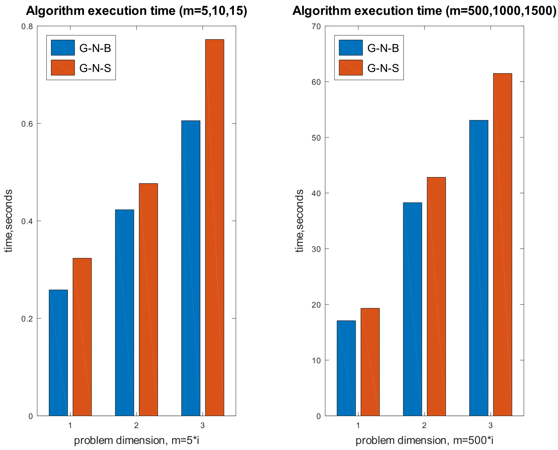
The diagrams in Figure 1 show the average execution time of the Gauss–Newton–Broyden and Gauss–Newton–Secant algorithms for low- and high-dimensional problems (Example 4). Each algorithm was run 10 times, after which the average execution time was calculated. The results were obtained for the initial approximation $x_0={(0.4,6,0.5)}^{\top }$. The number of iterations is 14 ($m=5,10,15$) and 15 ($m=500,1000,1500$) for the Gauss–Newton–Broyden method and 12 ($m=500,1000,1500$) and 13 ($m=5,10,15$) for the Gauss–Newton–Secant method. Despite the fact that the Gauss–Newton–Broyden method requires more iterations for convergence, its overall execution time is shorter. This behavior is typically observed when the difference between the number of iterations of the methods is not significant.

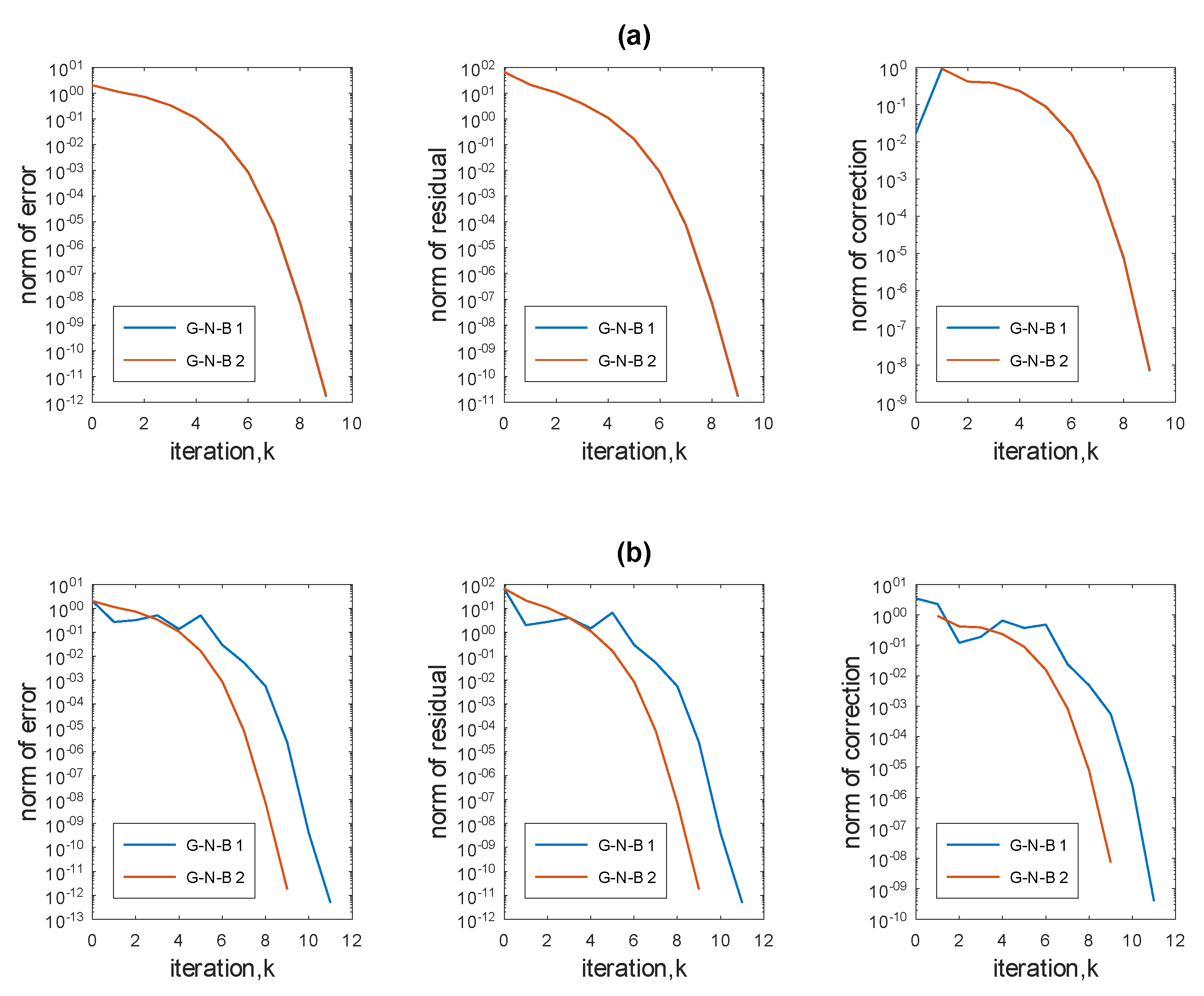
The graphs in Figure 2 show the influence of the initial approximation $B_0$ and $x_{-1}$ on the convergence of the Gauss–Newton–Broyden method (7). The initial approximation $x_0={(0.7,8,0.8)}^{\top }$. Two methods of specifying the matrix $B_0$ are considered: $G-N-B1$ means that $B_0=\mathcal{G}(x_0,x_{-1})$, and $G-N-B2$ means that the finite difference approximation $B_0(·,j)={\displaystyle \frac{\mathcal{G}(x_0+\delta e_j)-\mathcal{G}\left(x_0\right)}{\delta }},\delta ={10}^{-8}$ is used. In this case, $G-N-B1$ additionally depends on the initial approximation $x_{-1}$. From the obtained results, we see that, if $x_0$ and $x_{-1}$ are close enough (Figure 2a), the choice of $B_0$ has almost no effect on the results: at each iteration, the obtained values are quite close, and the errors smoothly decrease. If the initial approximations differ significantly (Figure 2b), and $B_0$ is calculated using method $G-N-B1$, the error graphs may have significant jumps, which can lead to divergence of the iterative process. Therefore, it is advisable to use additional mechanisms that ensure the direction of the iterative process to the solution.

We also applied the proposed Gauss–Newton–Broyden method (7) for solving nonlinear complementarity problems. The complementarity problem [8,25] consists of finding a vector $x\in R^n$ such that

$$x\ge 0,\Phi \left(x\right)\ge 0,and{x}^{\top }\Phi \left(x\right)=0,$$

(22)

where $\Phi :\mathrm{I}{\mathrm{R}}^{\mathrm{n}}\to \mathrm{I}{\mathrm{R}}^{\mathrm{n}}$ is a continuously differentiable linear or nonlinear function. It is known that this problem reduces to a system of nonlinear equations

$$\mathcal{H}\left(x\right)=\left(\begin{array}{c}\varphi (x_1,{\Phi }_1\left(x\right))\\ ⋮\\ \varphi (x_n,{\Phi }_n\left(x\right))\end{array}\right)=0,$$

(23)

where $\varphi (a,b)$ is some function. We chose it as a penalized Fischer–Burmeister function [25]

$$\varphi (a,b)=\lambda (a+b-\sqrt{a^2+b^2})+(1-\lambda )a_{+}{b}_{+},$$

where $a_{+}=\max \{0,a\}$, and $\lambda \in (0,1)$ is a fixed parameter. The methods were tested on two problems.

Example 5.

$n\ge 1,$ $\Phi \left(x\right)=Mx+q+E\left(x\right)$, where a matrix $M=diag\{1,1/2,\dots ,1/n\}$, a vector $q\in \mathrm{I}{\mathrm{R}}^{\mathrm{n}}$ with components $q_i=-3$, and nonlinear functions $E_i\left(x\right)=e^{x_i-2}+e^{x_{i+1}-3}$, $i=1,\dots ,n-1$, $E_n\left(x\right)=e^{x_n-2}$. This problem has a solution ${\kappa }^{*}$, such that $\mathcal{H}\left({\kappa }^{*}\right)={(0,\dots ,0)}^{\top }$.

Example 6.

$n=5,$

$$\begin{array}{c}\left\{\begin{array}{c}{\Phi }_1\left(x\right)=x_1+x_2{x}_3{x}_4{x}_5/50,\hfill \\ {\Phi }_2\left(x\right)=x_2+x_1{x}_3{x}_4{x}_5/50-3,\hfill \\ {\Phi }_3\left(x\right)=x_3+x_1{x}_2{x}_4{x}_5/50-1,\hfill \\ {\Phi }_4\left(x\right)=x_4+x_1{x}_2{x}_3{x}_5/50+0.5,\hfill \\ {\Phi }_5\left(x\right)=x_5+x_1{x}_2{x}_3{x}_4/50,\hfill \end{array}\right.\\ {\kappa }^{*}={(0,3,1,0,0)}^{\top },\Phi \left({\kappa }^{*}\right)={(0,0,0,0.5,0)}^{\top }.\end{array}$$

Table 3. Number of iterations for solving complementarity problems 5 and 6.

Example	$\mathit{\lambda }$	Method
		G-N-B	G-N-S	B
		(7)	(6)	(21)
	0.75	15	10	19
5	0.8	13	9	17
$n=10$	0.95	13	8	13
	0.3	14	5	12
6	0.5	6	5	7
	0.95	6	4	6

presents the results obtained for Examples 5 and 6. For Example 5, the initial approximation was $x_0={(1.5,\dots ,1.5)}^{\top }$; for Example 6, $x_0={\kappa }^{*}+{10}^{-2}$.

Table 4. Norm of residuals for Example 6.

k	G-N-B		G-N-S		B
	$\parallel \mathcal{H}\left({\mathit{x}}_{\mathit{k}}\right)\parallel$	$\parallel \mathbf{\Psi }\left({\mathit{x}}_{\mathit{k}}\right)\parallel$	$\parallel \mathcal{H}\left({\mathit{x}}_{\mathit{k}}\right)\parallel$	$\parallel \mathbf{\Psi }\left({\mathit{x}}_{\mathit{k}}\right)\parallel$	$\parallel \mathcal{H}\left({\mathit{x}}_{\mathit{k}}\right)\parallel$	$\parallel \mathbf{\Psi }\left({\mathit{x}}_{\mathit{k}}\right)\parallel$
1	$1.0883\times {10}^{-4}$	$1.4279\times {10}^{-4}$	$1.0883\times {10}^{-4}$	$1.4279\times {10}^{-4}$	$1.0878\times {10}^{-4}$	$1.4275\times {10}^{-4}$
2	$1.1868\times {10}^{-6}$	$9.6534\times {10}^{-7}$	$6.6968\times {10}^{-7}$	$1.2971\times {10}^{-6}$	$1.2098\times {10}^{-6}$	$9.5263\times {10}^{-7}$
3	$1.8907\times {10}^{-8}$	$5.1621\times {10}^{-8}$	$7.7605\times {10}^{-9}$	$1.1370\times {10}^{-9}$	$5.1812\times {10}^{-8}$	$5.2656\times {10}^{-8}$
4	$1.4541\times {10}^{-9}$	$1.3243\times {10}^{-9}$	$3.3724\times {10}^{-9}$	$5.6389\times {10}^{-12}$	$6.9717\times {10}^{-10}$	$1.2465\times {10}^{-9}$
5	$8.5122\times {10}^{-12}$	$1.3515\times {10}^{-11}$			$5.6317\times {10}^{-11}$	$1.6240\times {10}^{-11}$

shows the dynamics of the residuals norms. Here, $\Psi \left(x_k\right)$ is a vector with components ${\Psi }_i\left(x_k\right)={\zeta }_i{\Phi }_i\left(x_k\right)$ and $x_k={({\zeta }_1,\dots ,{\zeta }_n)}^{\top }$. The results are given for Example 6 and $\lambda =0.99$.

From the obtained results, we observe that quasi-Newton-type methods are highly sensitive to the choice of the parameter $\lambda$.

4. Conclusions

A Gauss–Newton–Broyden method for NLSP with the decomposition of the nonlinear operator is developed and analyzed. The proposed approach replaces the Jacobian matrix of the nonlinear vector function by the sum of the derivative of the differentiable part of the nonlinear function and a matrix computed using Broyden’s update formula for the remaining part of the function. Convergence analysis is provided under the classical Lipschitz conditions for zero-residual problems. The applicability of theoretical results has been confirmed. The numerical experiments demonstrate the effectiveness of the proposed approach.

References

1. Dennis, J.E.; Schnabel, R.B. Numerical Methods for Unconstrained Optimization and Nonlinear Equations; Prentice-Hall: Englewood Cliffs, NJ, USA, 1983. [Google Scholar]
2. Argyros, I.K. The Theory and Application of Iteration Methods, 2nd ed.; CRC Press: Boca Raton, FL, USA, 2022. [Google Scholar] [CrossRef] [Scilit]
3. Madsen, K.; Nielsen, H.; Tingleff, O. Methods for Non-Linear Least Squares Problems, 2nd ed.; Informatics and Mathematical Modelling Technical University of Denmark: Kongens Lyngby, Denmark, 2004; Volume 60. [Google Scholar]
4. Kimiaei, M.; Neumaier, A. A new limited memory method for unconstrained nonlinear least squares. Soft Comput. 2022, 26, 465–490. [Google Scholar] [CrossRef] [Scilit] [PubMed]
5. Shakhno, S.M. Iterative methods for solving nonlinear least squares problems. J. Numer. Appl. Math. 2013, 1, 154–169. (In Ukrainian) [Google Scholar]
6. Wang, S.; Xu, M.; Zhang, X.; Wang, Y. Fitting nonlinear equations with the Levenberg–Marquardt method on Google Earth Engine. Remote Sens. 2022, 14, 2055. [Google Scholar] [CrossRef] [Scilit]
7. Śmietański, M.J. On a Nonsmooth Gauss–Newton Algorithms for Solving Nonlinear Complementarity Problems. Algorithms 2020, 13, 190. [Google Scholar] [CrossRef] [Scilit]
8. Ma, C.; Jiang, L.; Wang, D. The convergence of a smoothing damped Gauss–Newton method for nonlinear complementarity problem. Nonlinear Anal. Real World Appl. 2009, 10, 2072–2087. [Google Scholar] [CrossRef] [Scilit]
9. Pérez, R.; Sánchez, W.; Martínez, H.J. On the local convergence of a smoothing structured secant method for nonlinear complementarity. Appl. Math. Comput. 2025, 488, 129095. [Google Scholar] [CrossRef] [Scilit]
10. Florez, H.; Argáez, M. A Reduced-Order Gauss-Newton Method for Nonlinear Problems Based on Compressed Sensing for PDE Applications. In Nonlinear Systems—Modeling, Estimation, and Stability; InTech: London, UK, 2018. [Google Scholar] [CrossRef] [Scilit]
11. Guo, H.; Liu, G.; Wang, L. An improved Tikhonov-regularized variable projection algorithm for separable nonlinear least squares. Axioms 2021, 10, 196. [Google Scholar] [CrossRef] [Scilit]
12. Ortega, J.M.; Rheinboldt, W.C. Iterative Solution of Nonlinear Equations in Several Variables; Academic Press: New York, NY, USA, 1970. [Google Scholar]
13. Argyros, I.K.; George, S. Local convergence of a two-step Gauss-Newton Werner-type method for solving least squares problems. J. Numer. Anal. Approx. Theory 2024, 53, 52–62. [Google Scholar] [CrossRef] [Scilit]
14. Wang, L.; Liu, G. A method for solving ill-conditioned nonlinear least squares problems and its application in image distortion correction using self-calibration. Axioms 2024, 13, 209. [Google Scholar] [CrossRef] [Scilit]
15. Grau-Sánchez, M.; Noguera, M.; Amat, S. On the approximation of derivatives using divided difference operators preserving the local convergence order of iterative methods. J. Comput. Appl. Math. 2013, 237, 363–372. [Google Scholar] [CrossRef] [Scilit]
16. Ren, H.; Argyros, I.K. Local convergence of a secant type method for solving least squares problems. Appl. Math. Comp. 2010, 217, 3816–3824. [Google Scholar] [CrossRef] [Scilit]
17. Piro, M.H.A.; Bell, J.S.; Poschmann, M.; Prudil, A.; Chan, P. A Jacobian free deterministic method for solving inverse problems. arXiv 2022, arXiv:2203.04138. [Google Scholar] [CrossRef] [Scilit]
18. Chen, X. On the convergence of Broyden-like methods for nonlinear equations with nondifferentiable terms. Ann. Inst. Stat. Math. 1990, 42, 387–401. [Google Scholar] [CrossRef] [Scilit]
19. Dennis, J.E. On the Convergence of Broyden’s Method for Nonlinear Systems of Equations. Math. Comp. 1971, 25, 559–567. [Google Scholar] [CrossRef] [Scilit][Green Version]
20. Argyros, I.K.; Shakhno, S.; Shunkin, Y. Improved convergence analysis of Gauss-Newton-Secant method for solving nonlinear least squares problems. Mathematics 2019, 7, 99. [Google Scholar] [CrossRef] [Scilit]
21. Shakhno, S.M.; Yarmola, H.P.; Shunkin, Y.V. Convergence analysis of the Gauss-Newton-Potra method for nonlinear least squares problems. Mat. Stud. 2018, 50, 211–221. [Google Scholar] [CrossRef] [Scilit]
22. Shakhno, S.M.; Yarmola, H.P. Local convergence of the Gauss-Newton-Kurchatov method under generalized Lipschitz conditions. Carpathian Math. Publ. 2021, 13, 305–314. [Google Scholar] [CrossRef] [Scilit]
23. Shakhno, S.; Yarmola, H. On the Newton-Broyden method for solving systems of nonlinear equations. JANA 2023, 1, 80–87. [Google Scholar] [CrossRef] [Scilit]
24. Cătinaş, E. On some iterative methods for solving nonlinear equations. Rev. Anal. Numer. Theor. Approx. 1994, 23, 47–53. [Google Scholar] [CrossRef]
25. Tawhid, M.A. Unconstrained methods for nonsmooth nonlinear complementarity problems. Adv. Model. Optim. 2010, 12, 20–35. [Google Scholar]
Figure 1. Average execution time of algorithms for Example 4 * with dimensions m = 5 i and m = 500 i , i = 1 , 2 , 3 .
Axioms 15 00682 g001
Figure 2. Results for different initial approximations (Example 4): (a) – x 1 = x 0 + 0.01 , (b) – x 1 = x 0 + 2 .
Axioms 15 00682 g002