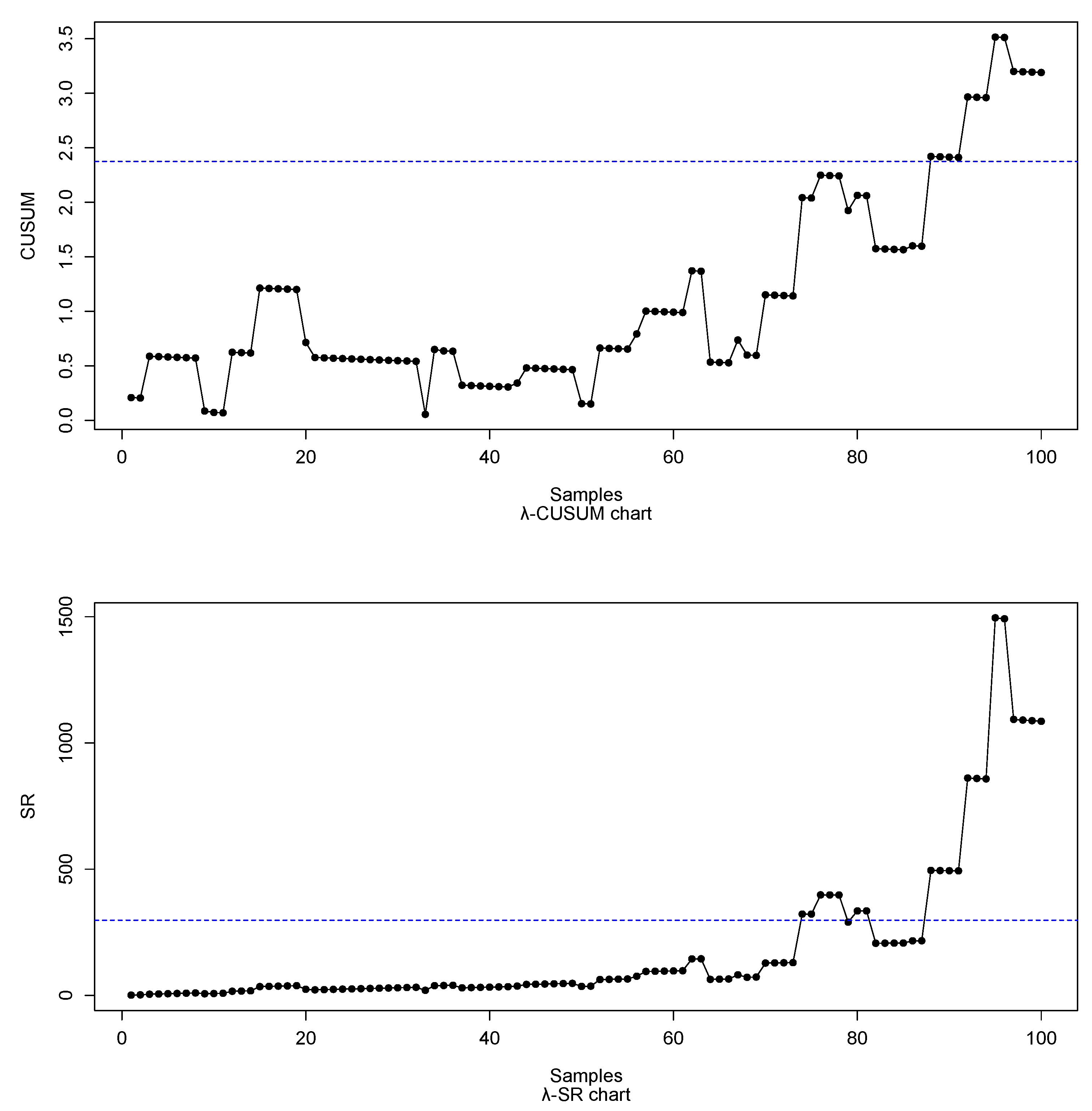
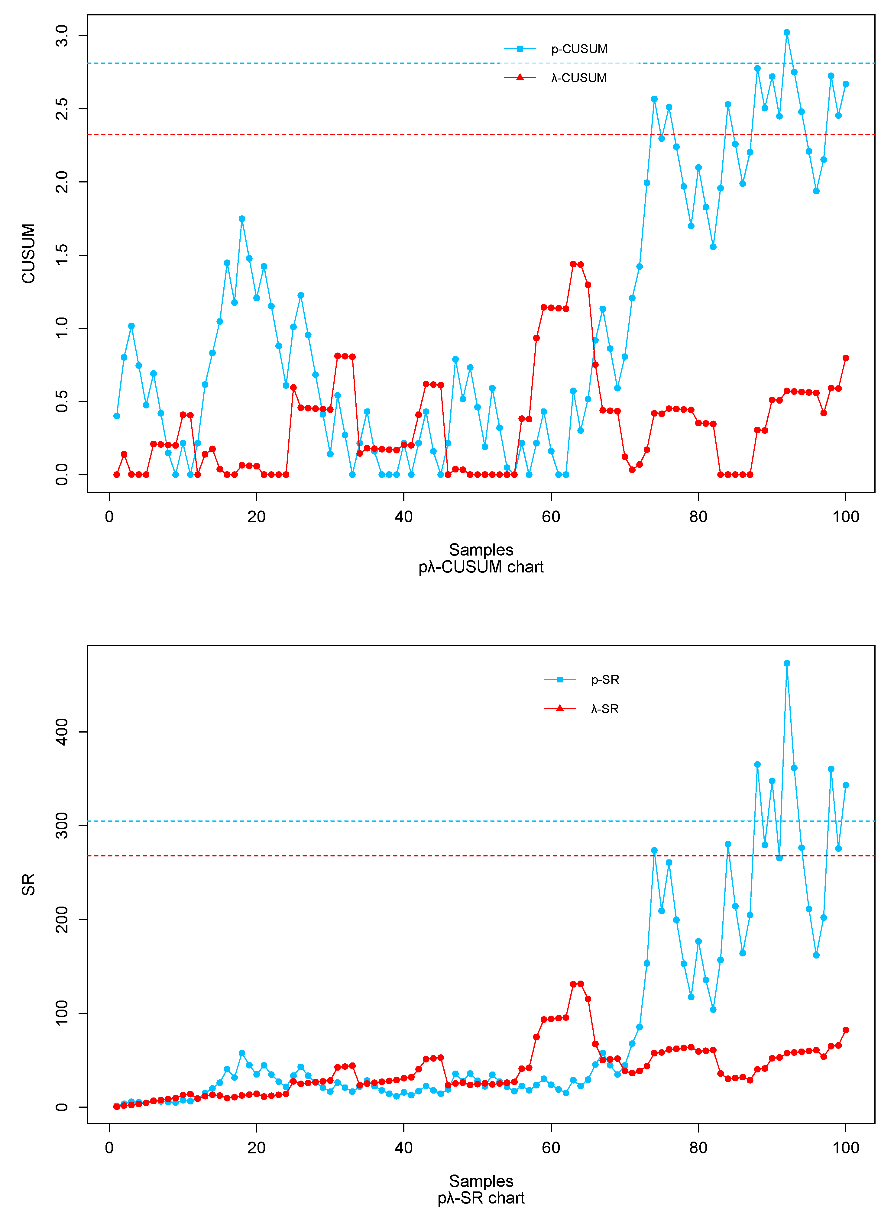
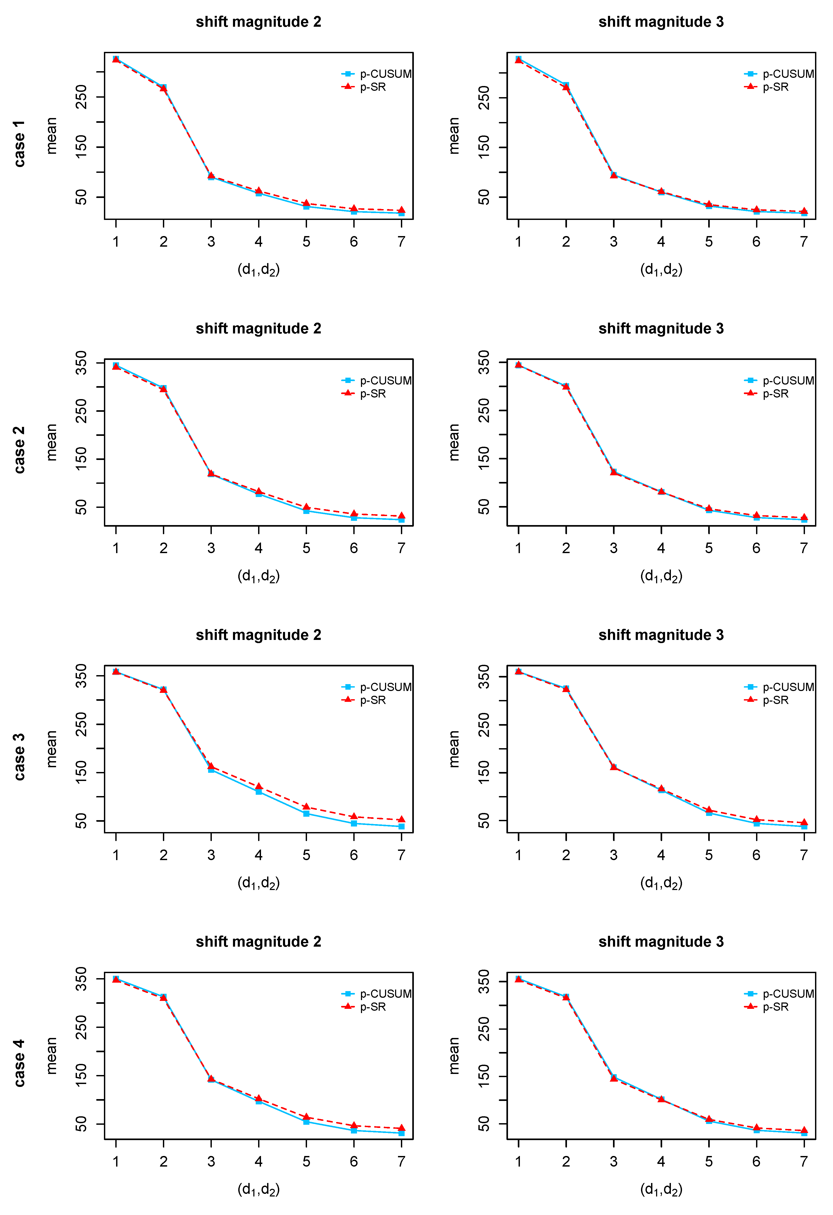
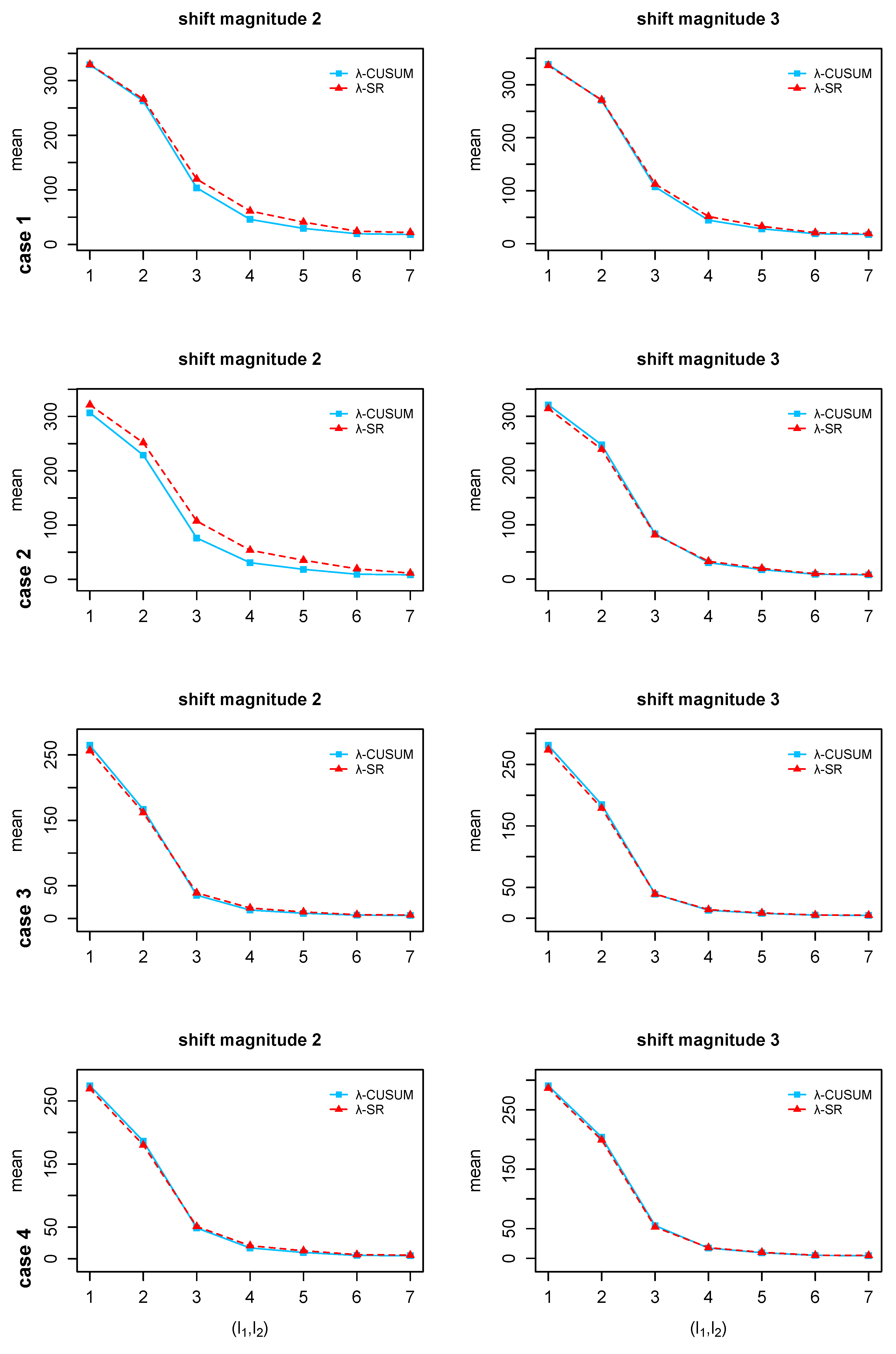
A Comparison of Shiryaev–Roberts and Cumulative Sum Procedures for Bivariate ZIP Process Monitoring


Abstract
1. Introduction
2. Background and Existing Research
2.1. Bivariate Zero-Inflated Poisson Distribution
2.2. CUSUM Chart Proposed by He et al. [28]
2.2.1. The p-CUSUM Procedure for Monitoring Shifts in the p-Set Parameters
- = ln for with
- = ln for with
- = ln for with
- = ln for with
2.2.2. The -CUSUM Procedure for Monitoring Shifts in the -Set Parameters
- = ln for with
- = ln for with
- = ln for with
- = ln for with
3. The SR Control Procedure
3.1. The p-SR Procedure for Monitoring Shifts in the p-Set Parameters
- for ;
- for ;
- for ;
- for .
3.2. The -SR Procedure for Monitoring Shifts in the -Set Parameters
- for ;
- for ;
- for ;
- for .
3.3. The -SR Procedure for Simultaneously Monitoring Shifts Both in the p-Set and -Set Parameters with a Combination of the p-SR and -SR Procedures
4. Simulation Studies
- (1)
- = 0.89, = 0.03, = 0.03, = 0.05, = 2.0, = 2.0, = 1.5;
- (2)
- = 0.745, = 0.10, = 0.075, = 0.08, = 3.0, = 4.0, = 1.0;
- (3)
- = 0.63, = 0.135, = 0.135, = 0.10, = 1.0, = 1.0, = 0.5;
- (4)
- = 0.54, = 0.10, = 0.20, = 0.16, = 2.5, = 1.5, = 1.0.
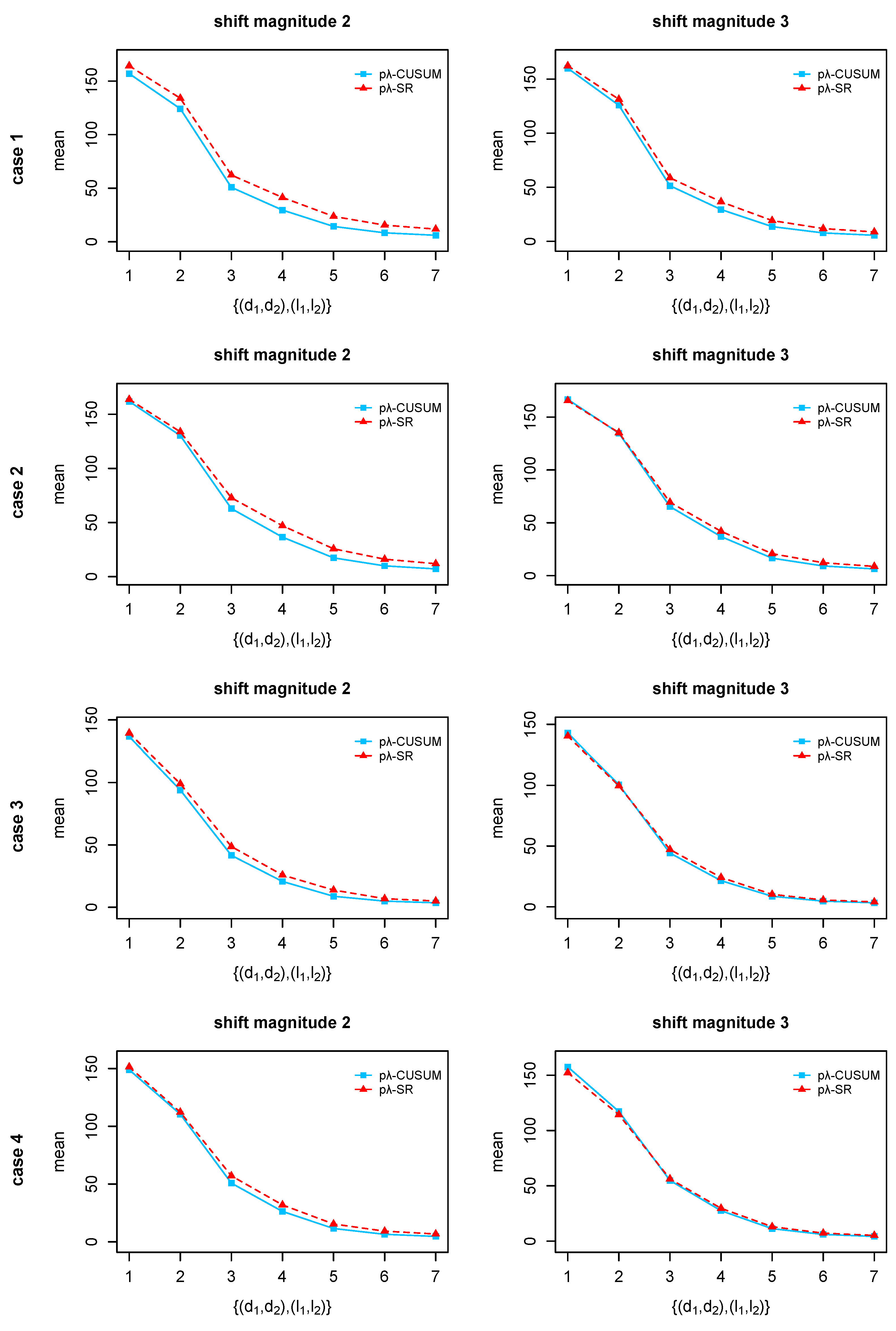
- shift magnitude 1: = , = , = , and = ;
- shift magnitude 2: = , = , = , and = ;
- shift magnitude 3: = , = , = , and = .
- shift magnitude 1: = , = , and = ;
- shift magnitude 2: = , = , and = ;
- shift magnitude 3: = , = , and = .
| Algorithm 1 Computing the control limits of the p-SR and -SR charts via Monte Carlo simulation with bisection |
|
| Algorithm 2 Determining the control limits of the -SR chart by Monte Carlo simulation |
|
| Algorithm 3 Obtaining the ARL1 of the p-SR, -SR and -SR charts via Monte Carlo simulation |
|
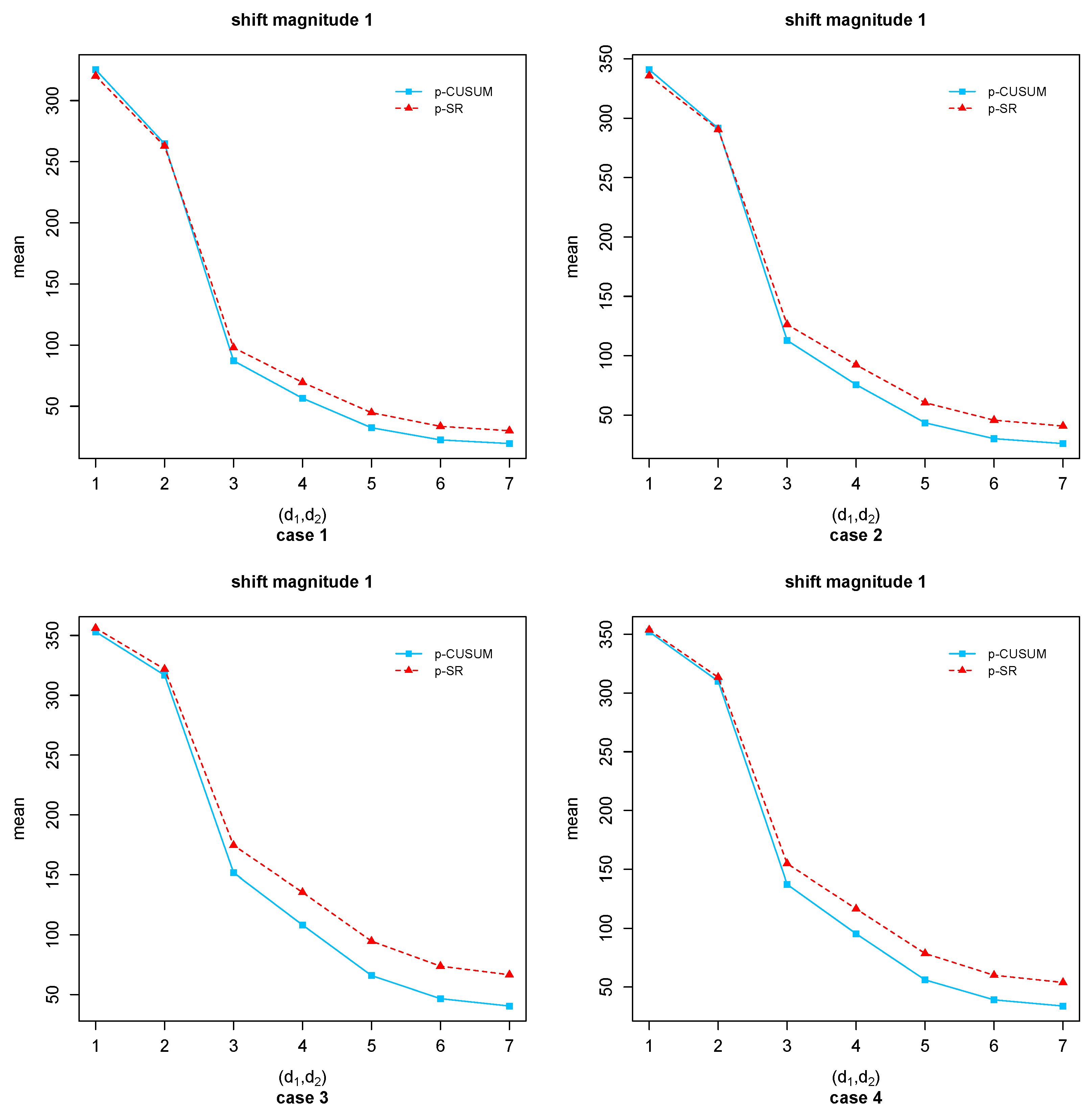
4.1. Individual Monitoring of p-Set Parameter Shifts
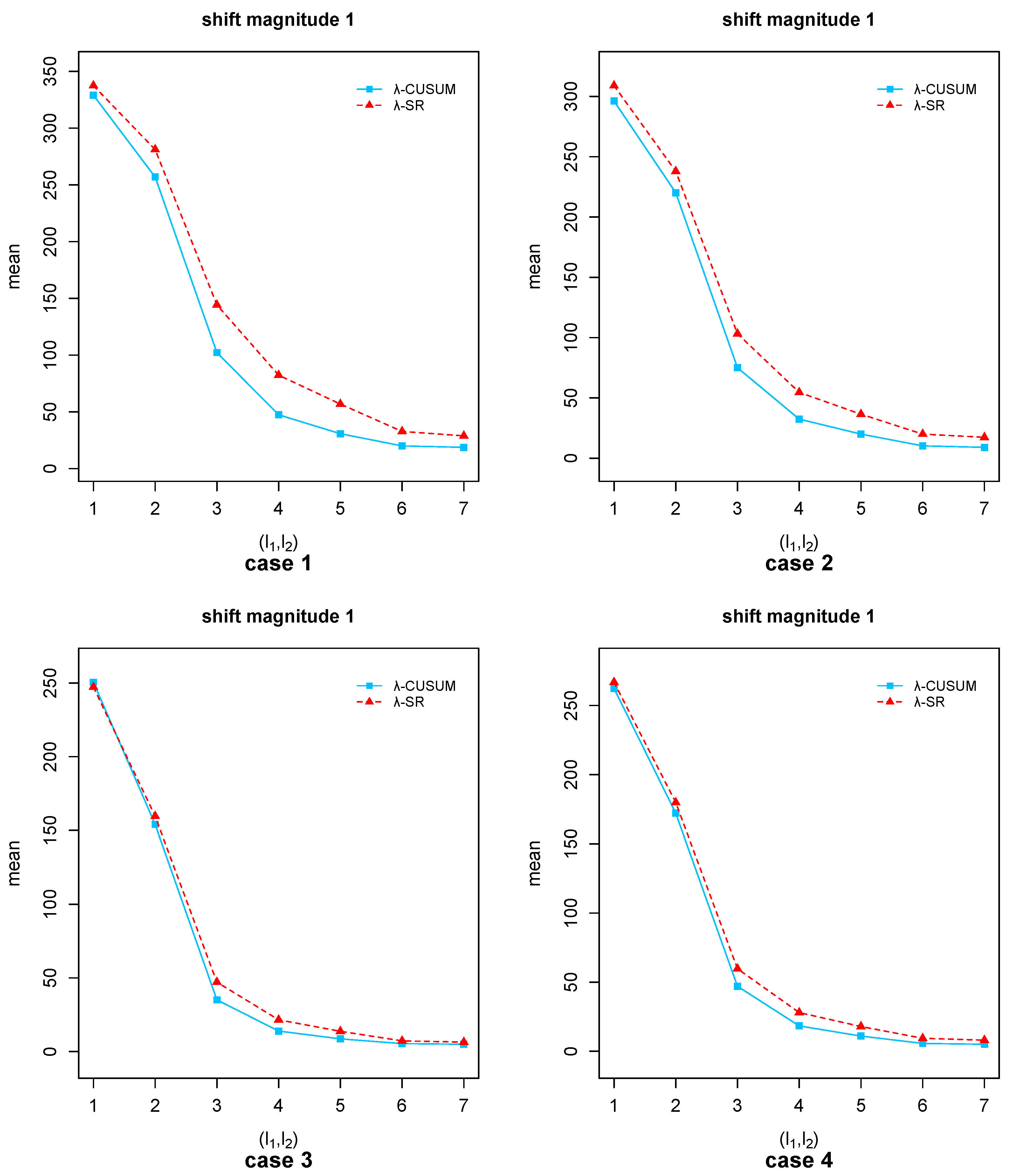
4.2. Individual Monitoring of -Set Parameter Shifts
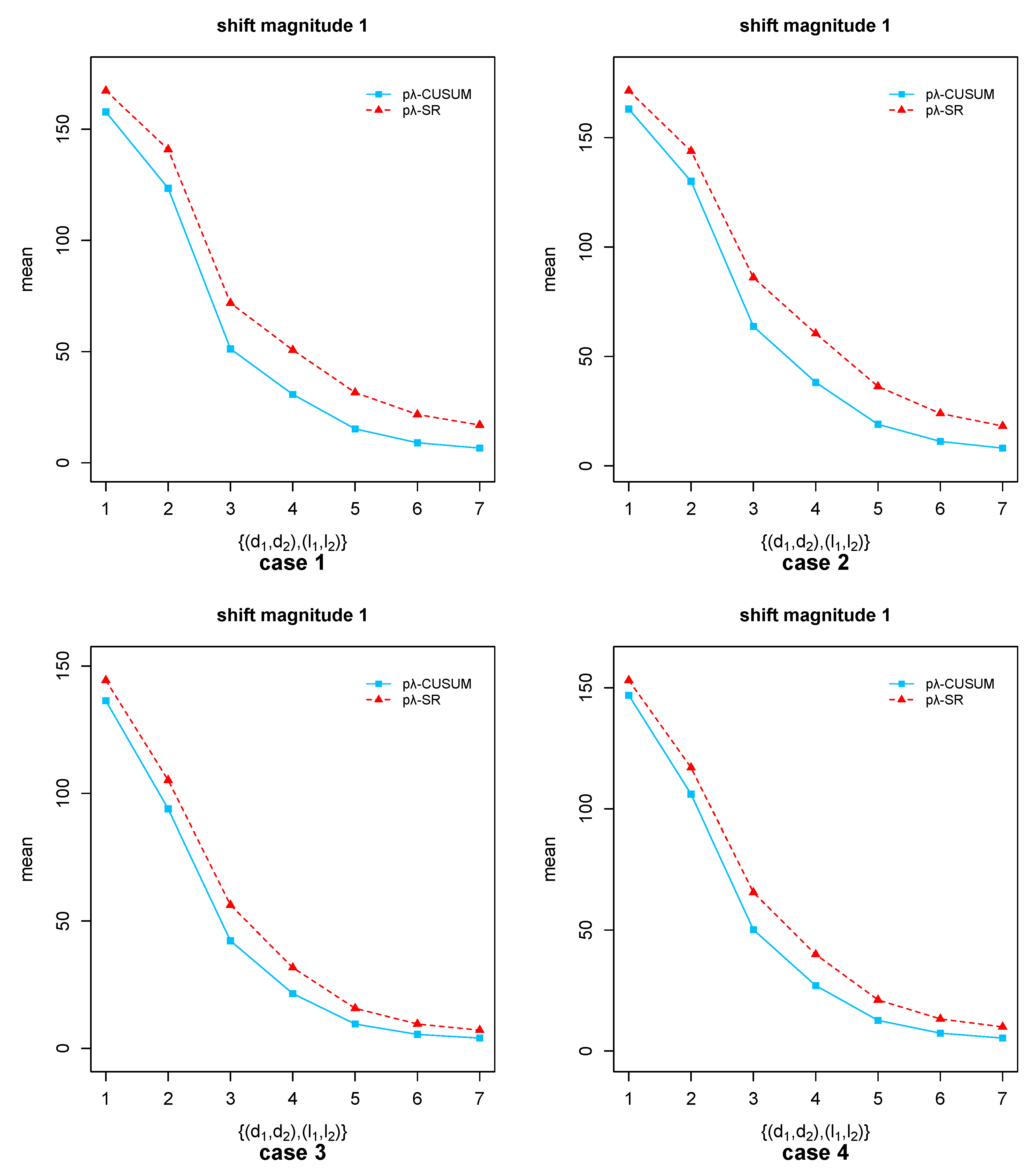
4.3. Simultaneously Monitoring Shifts Both in the p-Set and -Set Parameters with a Combination of the p-SR and -SR Procedures
4.4. Run-Length Performance of the Proposed SR Procedures
5. Sensitivity Analysis
5.1. Effect of Parameter Estimation for the SR Procedure with BZIP Model
5.2. Effect of the Independence Assumption for the SR Procedure with BZIP Model
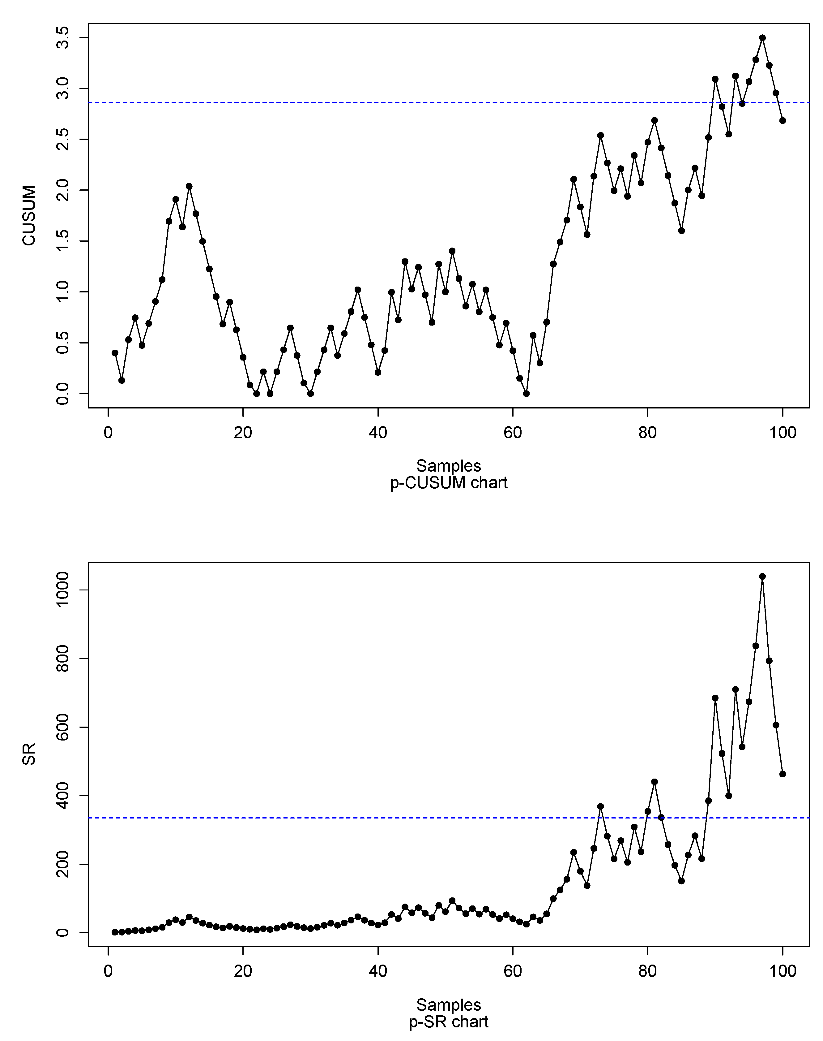
6. An Illustrative Example
7. Conclusions
Author Contributions
Funding
Data Availability Statement
Conflicts of Interest
Appendix A

| No. | Shift Magnitude | (,) | |||||||||||||||||||
|---|---|---|---|---|---|---|---|---|---|---|---|---|---|---|---|---|---|---|---|---|---|
| (0.006,0.001) | (0.012,0.002) | (0.06,0.003) | (0.09,0.004) | (0.15,0.005) | (0.21,0.006) | (0.24,0.007) | |||||||||||||||
| -CUSUM | -SR | -CUSUM | -SR | -CUSUM | -SR | -CUSUM | -SR | -CUSUM | -SR | -CUSUM | -SR | -CUSUM | -SR | ||||||||
| 1 | 1 | 397.31 | 397.61 | 403.90 | 399.78 | 397.90 | 399.42 | 402.79 | 398.03 | 403.05 | 398.23 | 400.73 | 399.86 | 403.80 | 397.12 | ||||||
| 2 | 328.86 | 298.54 | 275.86 | 257.97 | 116.40 | 107.91 | 75.95 | 75.59 | 42.71 | 45.89 | 28.77 | 32.61 | 24.81 | 28.45 | |||||||
| 3 | 317.22 | 292.41 | 263.10 | 241.47 | 91.79 | 89.72 | 60.42 | 61.34 | 33.10 | 36.62 | 22.76 | 26.22 | 19.56 | 23.01 | |||||||
| 4 | 317.73 | 289.66 | 269.37 | 244.92 | 94.96 | 92.55 | 60.94 | 62.75 | 34.18 | 37.69 | 22.84 | 26.97 | 19.83 | 23.22 | |||||||
| 5 | 318.10 | 290.43 | 271.67 | 250.12 | 101.76 | 98.53 | 68.03 | 68.10 | 37.40 | 40.79 | 25.23 | 28.80 | 21.91 | 25.47 | |||||||
| 6 | 326.87 | 293.46 | 271.56 | 250.36 | 103.63 | 98.83 | 68.67 | 69.04 | 38.61 | 41.06 | 25.78 | 29.19 | 22.10 | 25.60 | |||||||
| 7 | 311.76 | 288.75 | 262.56 | 241.23 | 93.46 | 90.43 | 60.17 | 62.48 | 33.96 | 37.18 | 22.89 | 26.47 | 19.62 | 22.99 | |||||||
| 8 | 318.97 | 295.03 | 268.05 | 249.78 | 101.05 | 97.35 | 65.59 | 65.56 | 36.22 | 39.85 | 24.40 | 28.01 | 21.15 | 24.66 | |||||||
| 9 | 309.39 | 288.82 | 256.38 | 241.84 | 94.18 | 90.77 | 59.29 | 61.81 | 33.45 | 37.36 | 23.12 | 26.38 | 19.64 | 22.99 | |||||||
| 10 | 319.83 | 293.14 | 273.25 | 252.41 | 105.64 | 99.62 | 68.37 | 68.74 | 38.28 | 41.18 | 25.87 | 29.41 | 22.19 | 25.51 | |||||||
| 11 | 319.92 | 298.28 | 278.15 | 252.51 | 103.80 | 98.23 | 68.43 | 67.82 | 37.68 | 40.46 | 25.55 | 29.08 | 21.98 | 25.21 | |||||||
| mean | 318.87 | 292.85 | 268.99 | 248.26 | 100.67 | 96.39 | 65.59 | 66.32 | 36.56 | 39.81 | 24.72 | 28.31 | 21.28 | 24.71 | |||||||
| 1 | 2 | 400.76 | 402.44 | 398.15 | 397.44 | 399.88 | 398.05 | 397.65 | 398.27 | 398.45 | 401.82 | 400.09 | 403.90 | 403.16 | 400.78 | ||||||
| 2 | 336.78 | 319.03 | 296.17 | 273.73 | 126.59 | 110.45 | 82.84 | 73.40 | 43.39 | 41.79 | 28.40 | 28.27 | 23.92 | 23.94 | |||||||
| 3 | 325.87 | 302.78 | 276.21 | 255.91 | 100.31 | 91.40 | 63.53 | 59.80 | 33.35 | 33.05 | 21.96 | 22.40 | 18.72 | 19.32 | |||||||
| 4 | 323.19 | 305.92 | 281.46 | 260.63 | 103.19 | 92.75 | 64.65 | 61.47 | 34.67 | 33.94 | 22.67 | 23.25 | 19.45 | 19.96 | |||||||
| 5 | 327.79 | 312.99 | 289.22 | 261.69 | 111.00 | 99.57 | 72.82 | 64.81 | 38.75 | 37.19 | 24.90 | 25.09 | 21.13 | 21.79 | |||||||
| 6 | 329.87 | 313.73 | 292.09 | 265.28 | 114.59 | 102.10 | 72.63 | 66.51 | 38.97 | 37.72 | 25.32 | 25.63 | 21.46 | 21.79 | |||||||
| 7 | 322.10 | 304.31 | 281.19 | 261.35 | 101.10 | 92.96 | 65.56 | 59.92 | 34.20 | 33.45 | 22.64 | 22.93 | 19.38 | 19.68 | |||||||
| 8 | 325.77 | 316.13 | 281.49 | 262.55 | 108.53 | 97.63 | 69.52 | 64.00 | 36.76 | 36.12 | 24.23 | 24.45 | 20.12 | 21.17 | |||||||
| 9 | 323.54 | 304.30 | 276.82 | 255.59 | 99.70 | 91.51 | 65.08 | 60.07 | 34.29 | 33.44 | 22.22 | 22.91 | 19.04 | 19.73 | |||||||
| 10 | 335.75 | 307.76 | 293.25 | 264.83 | 112.95 | 101.99 | 73.16 | 67.08 | 39.24 | 37.82 | 25.00 | 25.41 | 21.40 | 21.74 | |||||||
| 11 | 332.67 | 314.80 | 285.17 | 262.59 | 110.47 | 101.33 | 71.90 | 66.50 | 38.38 | 36.98 | 25.43 | 25.44 | 21.13 | 21.75 | |||||||
| mean | 328.33 | 310.17 | 285.31 | 262.41 | 108.84 | 98.17 | 70.17 | 64.35 | 37.20 | 36.15 | 24.28 | 24.58 | 20.58 | 21.09 | |||||||
| 1 | 3 | 398.19 | 402.11 | 399.11 | 398.19 | 398.30 | 397.96 | 399.86 | 400.17 | 397.17 | 399.61 | 398.12 | 402.05 | 399.92 | 400.59 | ||||||
| 2 | 338.37 | 334.73 | 306.03 | 293.80 | 135.71 | 121.37 | 90.85 | 78.06 | 46.23 | 42.53 | 28.69 | 27.96 | 23.94 | 23.43 | |||||||
| 3 | 336.55 | 321.25 | 285.40 | 270.65 | 108.23 | 98.98 | 67.90 | 62.22 | 35.13 | 32.92 | 22.56 | 22.31 | 18.69 | 18.49 | |||||||
| 4 | 331.69 | 319.14 | 285.58 | 276.65 | 109.03 | 100.72 | 70.67 | 64.61 | 36.57 | 34.31 | 22.87 | 22.57 | 19.20 | 19.09 | |||||||
| 5 | 336.41 | 323.97 | 288.39 | 281.77 | 120.17 | 107.62 | 78.32 | 70.54 | 39.46 | 37.90 | 25.60 | 24.67 | 21.16 | 20.50 | |||||||
| 6 | 337.97 | 325.84 | 290.42 | 280.17 | 121.59 | 110.73 | 77.77 | 71.68 | 40.99 | 38.26 | 25.75 | 24.50 | 21.10 | 21.02 | |||||||
| 7 | 329.71 | 315.13 | 280.25 | 276.71 | 109.26 | 98.51 | 68.69 | 63.57 | 35.38 | 34.28 | 22.68 | 22.30 | 19.17 | 18.89 | |||||||
| 8 | 335.77 | 316.62 | 286.96 | 281.25 | 117.32 | 104.22 | 75.77 | 68.74 | 39.22 | 36.29 | 24.21 | 24.13 | 20.33 | 20.39 | |||||||
| 9 | 331.87 | 310.85 | 288.42 | 269.10 | 108.80 | 98.61 | 68.84 | 63.83 | 34.90 | 34.09 | 22.49 | 21.96 | 19.18 | 18.62 | |||||||
| 10 | 343.06 | 332.59 | 293.00 | 285.54 | 122.70 | 111.38 | 78.48 | 71.42 | 40.92 | 38.39 | 25.91 | 24.77 | 21.24 | 21.23 | |||||||
| 11 | 329.95 | 331.47 | 295.94 | 282.47 | 119.64 | 108.95 | 76.95 | 70.64 | 40.45 | 38.11 | 25.44 | 24.21 | 21.35 | 20.95 | |||||||
| mean | 335.13 | 323.16 | 290.04 | 279.81 | 117.24 | 106.11 | 75.42 | 68.53 | 38.93 | 36.71 | 24.62 | 23.94 | 20.54 | 20.26 | |||||||
| No. | Shift Magnitude | (,) | |||||||||||||||||||
|---|---|---|---|---|---|---|---|---|---|---|---|---|---|---|---|---|---|---|---|---|---|
| (0.006,0.001) | (0.012,0.002) | (0.06,0.003) | (0.09,0.004) | (0.15,0.005) | (0.21,0.006) | (0.24,0.007) | |||||||||||||||
| -CUSUM | -SR | -CUSUM | -SR | -CUSUM | -SR | -CUSUM | -SR | -CUSUM | -SR | -CUSUM | -SR | -CUSUM | -SR | ||||||||
| 1 | 1 | 397.98 | 398.76 | 397.58 | 399.87 | 403.77 | 398.93 | 402.33 | 399.98 | 398.94 | 401.23 | 397.25 | 398.81 | 398.41 | 403.15 | ||||||
| 2 | 325.03 | 316.27 | 299.72 | 280.81 | 147.97 | 145.45 | 104.18 | 110.14 | 62.00 | 72.35 | 42.64 | 53.72 | 36.94 | 47.16 | |||||||
| 3 | 329.40 | 313.62 | 297.13 | 278.20 | 145.62 | 149.40 | 104.47 | 111.82 | 61.97 | 72.30 | 43.09 | 53.52 | 36.90 | 47.12 | |||||||
| 4 | 318.38 | 295.33 | 279.27 | 261.73 | 111.67 | 118.85 | 75.22 | 84.76 | 43.51 | 54.93 | 30.22 | 39.97 | 26.33 | 35.16 | |||||||
| 5 | 329.59 | 313.96 | 302.00 | 279.72 | 146.54 | 146.40 | 105.39 | 110.54 | 62.68 | 71.69 | 42.99 | 53.38 | 36.61 | 47.32 | |||||||
| 6 | 322.72 | 309.11 | 285.15 | 273.69 | 125.29 | 131.17 | 87.51 | 97.55 | 50.82 | 63.07 | 35.67 | 45.55 | 30.58 | 40.07 | |||||||
| 7 | 324.75 | 307.55 | 288.23 | 271.03 | 129.11 | 131.41 | 89.26 | 97.68 | 51.83 | 62.33 | 35.58 | 46.02 | 30.87 | 40.45 | |||||||
| 8 | 323.27 | 308.61 | 287.65 | 276.39 | 135.34 | 134.96 | 91.35 | 100.83 | 54.86 | 65.56 | 37.86 | 47.64 | 32.70 | 42.55 | |||||||
| 9 | 326.57 | 304.07 | 279.04 | 270.85 | 126.34 | 130.30 | 87.54 | 96.86 | 51.75 | 61.95 | 35.03 | 45.48 | 30.64 | 40.46 | |||||||
| 10 | 324.51 | 302.66 | 286.37 | 267.68 | 126.18 | 129.34 | 86.81 | 97.10 | 51.75 | 61.96 | 35.09 | 45.25 | 30.90 | 40.26 | |||||||
| 11 | 332.01 | 316.28 | 302.73 | 282.22 | 148.65 | 147.89 | 107.92 | 112.15 | 62.97 | 73.34 | 43.73 | 53.96 | 37.37 | 48.10 | |||||||
| mean | 325.62 | 308.75 | 290.73 | 274.23 | 134.27 | 136.52 | 93.97 | 101.94 | 55.41 | 65.95 | 38.19 | 48.45 | 32.98 | 42.86 | |||||||
| 1 | 2 | 398.08 | 397.71 | 401.29 | 398.86 | 397.20 | 402.26 | 398.60 | 397.20 | 400.55 | 402.87 | 398.69 | 399.80 | 401.03 | 403.93 | ||||||
| 2 | 339.68 | 317.89 | 314.55 | 284.90 | 158.80 | 145.07 | 108.50 | 101.72 | 64.59 | 62.96 | 43.06 | 44.47 | 36.53 | 38.58 | |||||||
| 3 | 344.87 | 322.46 | 309.37 | 288.74 | 153.33 | 143.82 | 109.70 | 103.91 | 63.64 | 62.71 | 42.50 | 44.25 | 36.81 | 38.40 | |||||||
| 4 | 328.63 | 308.31 | 281.63 | 264.78 | 119.25 | 110.06 | 79.67 | 74.88 | 44.03 | 46.05 | 29.90 | 32.37 | 25.64 | 27.78 | |||||||
| 5 | 338.44 | 321.38 | 315.78 | 291.52 | 153.32 | 142.14 | 110.22 | 102.01 | 63.43 | 62.89 | 43.06 | 43.93 | 36.24 | 38.33 | |||||||
| 6 | 332.41 | 312.55 | 292.92 | 280.76 | 133.77 | 124.30 | 91.75 | 86.93 | 52.06 | 52.01 | 35.64 | 37.28 | 30.09 | 32.28 | |||||||
| 7 | 332.48 | 317.10 | 294.34 | 276.98 | 136.95 | 123.37 | 91.04 | 87.76 | 52.36 | 52.22 | 34.98 | 37.26 | 30.28 | 32.59 | |||||||
| 8 | 335.31 | 311.34 | 302.81 | 278.73 | 139.33 | 131.61 | 95.78 | 90.86 | 55.78 | 55.57 | 37.41 | 38.93 | 32.08 | 34.24 | |||||||
| 9 | 339.54 | 315.40 | 297.39 | 274.84 | 133.35 | 123.68 | 90.46 | 86.95 | 51.39 | 52.68 | 35.16 | 36.77 | 29.80 | 32.32 | |||||||
| 10 | 330.65 | 312.23 | 293.58 | 278.69 | 134.44 | 122.63 | 91.09 | 87.91 | 51.91 | 52.12 | 34.77 | 37.16 | 30.12 | 31.99 | |||||||
| 11 | 348.76 | 322.84 | 309.89 | 292.98 | 159.09 | 147.06 | 112.19 | 102.11 | 64.73 | 62.55 | 43.99 | 45.04 | 37.22 | 39.01 | |||||||
| mean | 337.08 | 316.15 | 301.23 | 281.29 | 142.16 | 131.38 | 98.04 | 92.51 | 56.39 | 56.18 | 38.05 | 39.75 | 32.48 | 34.55 | |||||||
| 1 | 3 | 401.76 | 400.06 | 402.28 | 403.41 | 402.79 | 400.66 | 401.48 | 402.26 | 399.90 | 403.97 | 400.91 | 399.25 | 402.37 | 402.94 | ||||||
| 2 | 348.41 | 333.06 | 319.61 | 294.85 | 164.90 | 148.16 | 116.34 | 105.64 | 67.87 | 61.76 | 45.07 | 42.07 | 37.29 | 36.10 | |||||||
| 3 | 352.94 | 327.40 | 316.21 | 297.43 | 164.81 | 149.27 | 115.65 | 105.54 | 66.74 | 61.11 | 43.93 | 42.49 | 37.31 | 36.35 | |||||||
| 4 | 333.66 | 319.51 | 292.92 | 274.05 | 124.27 | 112.92 | 83.14 | 76.70 | 45.72 | 43.77 | 29.57 | 30.01 | 25.58 | 25.83 | |||||||
| 5 | 343.43 | 331.38 | 314.20 | 300.88 | 163.95 | 150.32 | 116.12 | 103.45 | 68.80 | 61.86 | 44.27 | 42.11 | 37.29 | 35.94 | |||||||
| 6 | 336.87 | 325.06 | 309.98 | 288.05 | 143.35 | 128.16 | 98.22 | 88.42 | 55.28 | 52.03 | 35.78 | 35.43 | 30.36 | 30.06 | |||||||
| 7 | 337.09 | 321.48 | 304.50 | 287.36 | 140.73 | 128.41 | 97.54 | 89.32 | 55.65 | 51.32 | 35.71 | 35.07 | 30.18 | 30.00 | |||||||
| 8 | 348.66 | 329.66 | 307.09 | 294.32 | 148.26 | 136.00 | 103.76 | 94.67 | 58.60 | 54.21 | 37.99 | 36.82 | 31.72 | 32.06 | |||||||
| 9 | 344.14 | 327.03 | 307.27 | 282.16 | 142.62 | 127.67 | 97.90 | 89.56 | 54.31 | 51.10 | 35.94 | 35.19 | 30.57 | 30.20 | |||||||
| 10 | 341.55 | 326.97 | 297.57 | 289.92 | 140.44 | 129.22 | 98.18 | 88.51 | 54.43 | 51.07 | 35.33 | 34.60 | 30.29 | 30.08 | |||||||
| 11 | 352.55 | 333.49 | 324.72 | 305.79 | 166.13 | 147.89 | 120.71 | 106.23 | 67.18 | 62.22 | 45.02 | 42.95 | 37.77 | 36.77 | |||||||
| mean | 343.93 | 327.50 | 309.41 | 291.48 | 149.94 | 135.80 | 104.76 | 94.80 | 59.46 | 55.04 | 38.86 | 37.67 | 32.84 | 32.34 | |||||||
| No. | Shift Magnitude | (,) | |||||||||||||||||||
|---|---|---|---|---|---|---|---|---|---|---|---|---|---|---|---|---|---|---|---|---|---|
| (0.006,0.001) | (0.012,0.002) | (0.06,0.003) | (0.09,0.004) | (0.15,0.005) | (0.21,0.006) | (0.24,0.007) | |||||||||||||||
| -CUSUM | -SR | -CUSUM | -SR | -CUSUM | -SR | -CUSUM | -SR | -CUSUM | -SR | -CUSUM | -SR | -CUSUM | -SR | ||||||||
| 1 | 1 | 401.65 | 403.50 | 402.66 | 397.72 | 398.83 | 401.98 | 399.19 | 402.84 | 400.28 | 402.07 | 398.56 | 401.16 | 398.23 | 402.91 | ||||||
| 2 | 312.73 | 300.70 | 267.10 | 252.23 | 98.51 | 102.34 | 64.79 | 70.79 | 36.19 | 43.47 | 25.04 | 31.53 | 21.83 | 27.59 | |||||||
| 3 | 337.22 | 320.03 | 305.49 | 287.70 | 158.31 | 149.35 | 110.25 | 109.32 | 64.27 | 70.43 | 43.22 | 50.53 | 36.83 | 43.82 | |||||||
| 4 | 325.87 | 301.41 | 280.97 | 266.22 | 114.44 | 113.76 | 76.26 | 81.39 | 42.27 | 49.28 | 28.90 | 35.73 | 24.92 | 31.28 | |||||||
| 5 | 332.53 | 311.36 | 284.95 | 265.62 | 120.62 | 121.35 | 81.80 | 86.23 | 46.64 | 53.82 | 32.07 | 38.58 | 27.29 | 33.77 | |||||||
| 6 | 311.97 | 298.46 | 270.01 | 255.46 | 105.57 | 108.55 | 69.58 | 75.57 | 39.35 | 46.56 | 26.90 | 33.70 | 23.10 | 29.44 | |||||||
| 7 | 331.78 | 319.09 | 293.05 | 274.91 | 130.17 | 130.45 | 89.08 | 92.88 | 52.33 | 57.64 | 35.15 | 41.66 | 30.14 | 36.64 | |||||||
| 8 | 318.43 | 308.24 | 279.39 | 265.36 | 119.14 | 118.35 | 80.99 | 85.05 | 45.29 | 52.46 | 30.66 | 37.87 | 26.58 | 33.11 | |||||||
| 9 | 333.42 | 311.23 | 292.01 | 276.26 | 133.93 | 130.91 | 93.11 | 95.24 | 52.55 | 58.51 | 35.17 | 42.45 | 30.58 | 37.22 | |||||||
| 10 | 316.26 | 295.80 | 269.39 | 252.86 | 104.10 | 106.75 | 68.52 | 74.55 | 39.31 | 46.49 | 26.75 | 33.20 | 22.94 | 28.96 | |||||||
| 11 | 322.84 | 308.53 | 289.29 | 270.68 | 121.02 | 122.00 | 83.55 | 87.36 | 46.88 | 54.12 | 31.73 | 39.12 | 27.56 | 34.19 | |||||||
| mean | 324.30 | 307.49 | 283.17 | 266.73 | 120.58 | 120.38 | 81.79 | 85.84 | 46.51 | 53.28 | 31.56 | 38.44 | 27.18 | 33.60 | |||||||
| 1 | 2 | 397.55 | 399.06 | 398.60 | 398.49 | 400.47 | 399.33 | 397.24 | 399.72 | 397.55 | 398.06 | 400.28 | 400.72 | 400.45 | 397.76 | ||||||
| 2 | 323.42 | 301.61 | 279.27 | 255.83 | 104.14 | 98.26 | 67.83 | 64.55 | 36.42 | 37.00 | 24.13 | 25.39 | 20.65 | 22.22 | |||||||
| 3 | 341.06 | 317.63 | 319.40 | 289.97 | 163.75 | 148.94 | 117.11 | 104.46 | 66.65 | 62.43 | 43.05 | 42.44 | 36.89 | 36.57 | |||||||
| 4 | 328.23 | 307.00 | 291.11 | 271.68 | 121.74 | 111.81 | 81.60 | 74.15 | 43.42 | 42.82 | 28.42 | 28.92 | 23.75 | 25.13 | |||||||
| 5 | 326.69 | 311.33 | 292.88 | 276.38 | 131.10 | 118.15 | 86.66 | 80.73 | 47.14 | 46.36 | 31.31 | 31.87 | 26.44 | 27.16 | |||||||
| 6 | 327.07 | 305.51 | 286.82 | 260.01 | 112.65 | 103.42 | 73.10 | 69.63 | 39.48 | 39.42 | 26.15 | 27.00 | 21.99 | 23.36 | |||||||
| 7 | 337.20 | 313.96 | 302.88 | 279.93 | 140.40 | 126.78 | 94.64 | 87.95 | 52.84 | 50.36 | 33.92 | 34.45 | 29.05 | 29.67 | |||||||
| 8 | 334.92 | 310.31 | 293.55 | 273.81 | 126.87 | 116.35 | 84.01 | 79.21 | 46.31 | 44.74 | 30.30 | 30.98 | 25.29 | 26.40 | |||||||
| 9 | 339.34 | 320.52 | 310.20 | 285.19 | 143.41 | 127.86 | 99.37 | 88.41 | 53.12 | 51.25 | 34.82 | 34.97 | 29.35 | 30.02 | |||||||
| 10 | 321.38 | 300.65 | 274.41 | 258.46 | 110.58 | 101.42 | 73.84 | 67.42 | 38.90 | 38.78 | 25.65 | 26.86 | 21.99 | 23.05 | |||||||
| 11 | 326.81 | 308.90 | 294.96 | 278.49 | 130.69 | 119.55 | 87.73 | 82.08 | 47.87 | 46.70 | 31.28 | 31.88 | 26.46 | 27.40 | |||||||
| mean | 330.61 | 309.74 | 294.55 | 272.97 | 128.53 | 117.25 | 86.59 | 79.86 | 47.22 | 45.99 | 30.90 | 31.48 | 26.19 | 27.10 | |||||||
| 1 | 3 | 397.93 | 401.95 | 402.84 | 397.37 | 403.39 | 402.00 | 402.42 | 398.49 | 401.57 | 400.81 | 399.76 | 401.70 | 399.75 | 398.25 | ||||||
| 2 | 332.56 | 315.76 | 289.22 | 276.06 | 113.68 | 106.25 | 73.90 | 68.66 | 38.04 | 37.21 | 24.72 | 24.57 | 20.45 | 21.04 | |||||||
| 3 | 354.99 | 338.21 | 327.06 | 312.37 | 179.64 | 157.83 | 127.14 | 110.24 | 71.58 | 64.17 | 45.47 | 41.90 | 37.13 | 35.25 | |||||||
| 4 | 342.78 | 325.40 | 304.22 | 289.02 | 132.37 | 119.43 | 86.78 | 77.29 | 45.62 | 41.95 | 28.25 | 27.76 | 23.72 | 23.39 | |||||||
| 5 | 343.26 | 326.30 | 305.71 | 288.72 | 144.14 | 126.70 | 94.26 | 85.56 | 50.10 | 46.78 | 32.58 | 31.07 | 26.49 | 26.38 | |||||||
| 6 | 331.67 | 321.20 | 294.53 | 278.49 | 122.02 | 111.15 | 78.51 | 72.29 | 41.21 | 39.19 | 26.41 | 25.95 | 22.24 | 22.25 | |||||||
| 7 | 354.09 | 331.24 | 313.57 | 302.14 | 156.07 | 138.73 | 104.51 | 92.33 | 56.02 | 51.27 | 35.35 | 33.80 | 29.04 | 28.22 | |||||||
| 8 | 333.43 | 321.87 | 307.53 | 289.81 | 137.67 | 123.71 | 91.05 | 82.61 | 48.60 | 45.38 | 30.55 | 29.42 | 25.43 | 25.57 | |||||||
| 9 | 349.13 | 339.45 | 314.77 | 305.70 | 154.41 | 141.41 | 106.18 | 93.72 | 56.15 | 52.11 | 35.18 | 34.20 | 29.60 | 28.90 | |||||||
| 10 | 333.81 | 322.55 | 289.64 | 271.45 | 117.47 | 109.38 | 78.72 | 71.70 | 40.71 | 38.81 | 25.92 | 25.41 | 21.72 | 21.84 | |||||||
| 11 | 342.76 | 325.92 | 302.86 | 291.31 | 144.42 | 127.90 | 93.24 | 84.85 | 50.50 | 47.25 | 31.95 | 31.17 | 26.59 | 26.08 | |||||||
| mean | 341.85 | 326.79 | 304.91 | 290.51 | 140.19 | 126.25 | 93.43 | 83.92 | 49.85 | 46.41 | 31.64 | 30.52 | 26.24 | 25.89 | |||||||
| No. | Shift Magnitude | (,) | |||||||||||||||||||
|---|---|---|---|---|---|---|---|---|---|---|---|---|---|---|---|---|---|---|---|---|---|
| (0.10,0.05) | (0.25,0.10) | (1.00,0.50) | (3.00,0.75) | (6.00,1.00) | (15.00,2.00) | (18.00,2.50) | |||||||||||||||
| -CUSUM | -SR | -CUSUM | -SR | -CUSUM | -SR | -CUSUM | -SR | -CUSUM | -SR | -CUSUM | -SR | -CUSUM | -SR | ||||||||
| 1 | 1 | 402.98 | 399.77 | 398.46 | 397.18 | 403.69 | 399.25 | 400.74 | 398.91 | 401.23 | 399.47 | 402.06 | 402.29 | 399.87 | 398.82 | ||||||
| 2 | 336.93 | 315.41 | 284.13 | 272.77 | 142.65 | 155.43 | 53.49 | 71.05 | 31.93 | 43.08 | 24.77 | 26.91 | 24.47 | 26.55 | |||||||
| 3 | 337.12 | 315.55 | 282.02 | 273.42 | 142.75 | 154.52 | 53.86 | 71.79 | 32.39 | 43.42 | 24.60 | 26.91 | 24.53 | 26.72 | |||||||
| 4 | 301.21 | 283.13 | 215.47 | 216.29 | 71.75 | 88.15 | 22.41 | 32.42 | 12.28 | 17.81 | 9.10 | 9.31 | 9.07 | 9.19 | |||||||
| 5 | 322.08 | 303.78 | 280.51 | 270.46 | 117.46 | 134.49 | 82.71 | 99.26 | 62.74 | 79.47 | 30.32 | 43.24 | 24.64 | 35.35 | |||||||
| 6 | 290.74 | 279.96 | 220.49 | 219.18 | 70.06 | 87.09 | 34.78 | 48.36 | 23.97 | 33.05 | 17.44 | 22.24 | 15.74 | 20.50 | |||||||
| 7 | 285.84 | 279.15 | 218.53 | 216.48 | 70.31 | 86.45 | 34.59 | 48.20 | 24.55 | 32.76 | 17.35 | 22.07 | 15.77 | 20.49 | |||||||
| 8 | 256.39 | 257.21 | 172.21 | 180.69 | 44.58 | 60.22 | 18.14 | 26.35 | 11.19 | 15.82 | 9.30 | 9.28 | 9.01 | 9.08 | |||||||
| mean | 304.33 | 290.60 | 239.05 | 235.61 | 94.22 | 109.48 | 42.85 | 56.78 | 28.44 | 37.92 | 18.98 | 22.85 | 17.60 | 21.13 | |||||||
| 1 | 2 | 402.65 | 397.58 | 397.46 | 399.69 | 403.99 | 398.85 | 401.87 | 397.75 | 402.47 | 397.73 | 401.92 | 403.87 | 398.43 | 397.76 | ||||||
| 2 | 345.15 | 317.31 | 295.45 | 267.50 | 151.07 | 138.02 | 53.91 | 55.43 | 31.30 | 33.21 | 24.64 | 24.81 | 24.74 | 25.09 | |||||||
| 3 | 347.52 | 316.06 | 298.43 | 268.95 | 147.90 | 140.05 | 53.75 | 55.69 | 30.61 | 33.07 | 24.76 | 24.92 | 24.67 | 24.87 | |||||||
| 4 | 312.79 | 284.79 | 230.80 | 209.12 | 72.83 | 73.43 | 21.55 | 23.46 | 11.87 | 12.73 | 9.02 | 9.24 | 8.92 | 9.01 | |||||||
| 5 | 334.33 | 311.78 | 287.97 | 269.98 | 123.88 | 115.83 | 85.52 | 81.44 | 63.47 | 63.14 | 29.17 | 31.56 | 23.48 | 25.49 | |||||||
| 6 | 301.73 | 273.07 | 232.01 | 206.80 | 72.67 | 70.03 | 34.35 | 35.83 | 23.74 | 24.86 | 17.18 | 18.29 | 15.59 | 16.53 | |||||||
| 7 | 302.86 | 274.39 | 226.05 | 212.37 | 69.78 | 70.31 | 33.72 | 35.91 | 23.88 | 25.22 | 17.50 | 17.85 | 15.58 | 16.19 | |||||||
| 8 | 280.76 | 244.98 | 183.66 | 167.97 | 44.50 | 45.72 | 16.99 | 18.71 | 10.77 | 11.60 | 9.08 | 9.12 | 9.11 | 9.03 | |||||||
| mean | 317.88 | 288.91 | 250.62 | 228.96 | 97.52 | 93.34 | 42.83 | 43.78 | 27.95 | 29.12 | 18.76 | 19.40 | 17.44 | 18.03 | |||||||
| 1 | 3 | 400.68 | 403.10 | 400.34 | 398.21 | 401.40 | 402.79 | 403.69 | 398.99 | 403.99 | 399.82 | 402.96 | 403.37 | 401.05 | 397.76 | ||||||
| 2 | 360.69 | 337.30 | 305.48 | 293.30 | 155.30 | 148.57 | 53.53 | 52.93 | 29.41 | 30.49 | 24.65 | 24.54 | 25.07 | 25.09 | |||||||
| 3 | 357.28 | 331.75 | 314.26 | 294.77 | 158.71 | 148.44 | 52.36 | 53.25 | 29.32 | 30.88 | 24.56 | 23.80 | 24.26 | 24.87 | |||||||
| 4 | 324.82 | 298.59 | 246.01 | 231.82 | 80.95 | 73.99 | 21.06 | 20.44 | 10.95 | 11.25 | 9.04 | 9.26 | 9.13 | 9.01 | |||||||
| 5 | 353.53 | 332.83 | 312.98 | 296.48 | 139.42 | 124.07 | 93.90 | 85.60 | 69.07 | 61.42 | 29.75 | 28.17 | 23.00 | 25.49 | |||||||
| 6 | 322.11 | 299.28 | 245.65 | 234.33 | 77.63 | 71.58 | 34.01 | 32.82 | 22.43 | 22.90 | 16.49 | 16.63 | 14.81 | 16.53 | |||||||
| 7 | 318.74 | 302.66 | 247.19 | 232.45 | 77.26 | 72.13 | 33.71 | 32.93 | 22.77 | 22.75 | 16.62 | 16.52 | 14.86 | 16.19 | |||||||
| 8 | 285.65 | 269.74 | 199.69 | 180.07 | 47.46 | 43.52 | 16.32 | 16.17 | 10.18 | 10.40 | 9.10 | 9.14 | 9.04 | 9.03 | |||||||
| mean | 331.83 | 310.31 | 267.32 | 251.89 | 105.25 | 97.47 | 43.56 | 42.02 | 27.73 | 27.16 | 18.60 | 18.29 | 17.17 | 18.03 | |||||||
| No. | Shift Magnitude | (,) | |||||||||||||||||||
|---|---|---|---|---|---|---|---|---|---|---|---|---|---|---|---|---|---|---|---|---|---|
| (0.10,0.05) | (0.25,0.10) | (1.00,0.50) | (3.00,0.75) | (6.00,1.00) | (15.00,2.00) | (18.00,2.50) | |||||||||||||||
| -CUSUM | -SR | -CUSUM | -SR | -CUSUM | -SR | -CUSUM | -SR | -CUSUM | -SR | -CUSUM | -SR | -CUSUM | -SR | ||||||||
| 1 | 1 | 397.55 | 398.30 | 399.10 | 398.38 | 401.80 | 399.76 | 400.89 | 397.15 | 398.24 | 397.47 | 402.41 | 401.55 | 398.98 | 397.10 | ||||||
| 2 | 295.92 | 278.22 | 222.87 | 213.79 | 79.81 | 89.80 | 25.77 | 33.71 | 14.08 | 18.97 | 8.29 | 10.30 | 7.81 | 9.24 | |||||||
| 3 | 317.05 | 304.96 | 264.29 | 250.14 | 123.22 | 125.34 | 41.46 | 51.30 | 21.76 | 29.03 | 11.48 | 15.35 | 10.72 | 13.52 | |||||||
| 4 | 261.47 | 251.58 | 171.15 | 168.33 | 46.76 | 56.01 | 14.16 | 19.63 | 7.58 | 10.27 | 4.22 | 5.26 | 4.01 | 4.69 | |||||||
| 5 | 304.58 | 292.22 | 256.84 | 245.81 | 92.43 | 99.64 | 59.23 | 71.02 | 44.06 | 54.50 | 21.09 | 28.22 | 16.71 | 22.84 | |||||||
| 6 | 250.00 | 242.67 | 166.85 | 163.97 | 40.52 | 50.39 | 17.60 | 23.94 | 10.83 | 14.63 | 6.59 | 8.10 | 6.20 | 7.22 | |||||||
| 7 | 273.14 | 253.86 | 191.35 | 191.13 | 51.61 | 61.78 | 23.59 | 31.04 | 14.45 | 19.69 | 8.01 | 10.54 | 7.41 | 9.18 | |||||||
| 8 | 221.93 | 215.05 | 129.45 | 134.48 | 29.35 | 37.75 | 11.52 | 15.73 | 6.67 | 8.99 | 4.08 | 4.87 | 3.99 | 4.44 | |||||||
| mean | 274.87 | 262.65 | 200.40 | 195.38 | 66.24 | 74.39 | 27.62 | 35.20 | 17.06 | 22.30 | 9.11 | 11.81 | 8.12 | 10.16 | |||||||
| 1 | 2 | 397.76 | 402.85 | 397.88 | 398.39 | 397.58 | 403.06 | 398.61 | 402.43 | 401.75 | 401.13 | 398.79 | 400.57 | 397.87 | 399.50 | ||||||
| 2 | 314.23 | 285.59 | 239.55 | 223.26 | 84.79 | 79.50 | 24.76 | 25.55 | 13.13 | 13.96 | 7.81 | 8.17 | 7.69 | 7.98 | |||||||
| 3 | 333.64 | 313.85 | 284.51 | 258.43 | 131.81 | 119.38 | 40.35 | 40.44 | 20.25 | 21.55 | 10.84 | 11.64 | 10.38 | 10.92 | |||||||
| 4 | 279.87 | 262.36 | 183.18 | 167.28 | 47.30 | 46.06 | 13.20 | 14.07 | 7.03 | 7.43 | 4.13 | 4.20 | 4.00 | 4.10 | |||||||
| 5 | 322.64 | 301.13 | 273.61 | 252.48 | 98.70 | 90.66 | 63.58 | 59.91 | 44.99 | 43.58 | 20.14 | 20.89 | 15.64 | 16.69 | |||||||
| 6 | 276.48 | 244.80 | 182.36 | 167.70 | 41.41 | 41.25 | 16.49 | 17.56 | 10.02 | 10.74 | 6.44 | 6.63 | 6.05 | 6.24 | |||||||
| 7 | 287.75 | 261.33 | 208.10 | 186.55 | 53.53 | 51.03 | 22.72 | 23.69 | 13.42 | 14.42 | 7.7 | 8.14 | 7.06 | 7.30 | |||||||
| 8 | 241.78 | 220.68 | 145.44 | 129.09 | 28.37 | 29.09 | 10.46 | 11.31 | 6.19 | 6.57 | 3.99 | 4.04 | 3.95 | 3.92 | |||||||
| mean | 293.77 | 269.96 | 216.68 | 197.83 | 69.42 | 65.28 | 27.37 | 27.50 | 16.43 | 16.89 | 8.72 | 9.10 | 7.82 | 8.16 | |||||||
| 1 | 3 | 397.76 | 401.01 | 400.81 | 400.22 | 402.65 | 403.57 | 401.44 | 398.75 | 400.37 | 402.31 | 401.38 | 403.16 | 400.65 | 398.51 | ||||||
| 2 | 337.10 | 317.12 | 265.42 | 250.91 | 97.69 | 88.56 | 25.32 | 24.11 | 12.32 | 12.17 | 7.92 | 7.86 | 7.63 | 7.55 | |||||||
| 3 | 364.87 | 342.34 | 309.23 | 288.35 | 149.08 | 135.91 | 42.25 | 39.86 | 18.81 | 19.23 | 10.76 | 10.88 | 10.20 | 10.38 | |||||||
| 4 | 309.50 | 284.41 | 213.59 | 191.74 | 55.83 | 48.87 | 12.63 | 12.39 | 6.20 | 6.24 | 4.02 | 4.02 | 3.90 | 3.96 | |||||||
| 5 | 337.53 | 329.57 | 304.19 | 281.29 | 116.63 | 103.75 | 74.40 | 65.65 | 50.49 | 46.39 | 20.30 | 19.39 | 14.93 | 14.97 | |||||||
| 6 | 296.19 | 274.55 | 202.84 | 189.21 | 45.01 | 42.50 | 16.10 | 15.51 | 9.28 | 9.22 | 6.27 | 6.28 | 5.95 | 5.91 | |||||||
| 7 | 310.36 | 296.59 | 233.24 | 211.39 | 61.95 | 54.84 | 22.54 | 21.49 | 12.52 | 12.54 | 7.52 | 7.49 | 6.90 | 6.77 | |||||||
| 8 | 262.33 | 244.93 | 165.10 | 151.42 | 30.82 | 28.44 | 9.75 | 9.80 | 5.55 | 5.45 | 3.88 | 3.98 | 3.90 | 3.95 | |||||||
| mean | 316.84 | 298.50 | 241.94 | 223.47 | 79.57 | 71.84 | 29.00 | 26.97 | 16.45 | 15.89 | 8.67 | 8.56 | 7.63 | 7.64 | |||||||
| No. | Shift Magnitude | (,) | |||||||||||||||||||
|---|---|---|---|---|---|---|---|---|---|---|---|---|---|---|---|---|---|---|---|---|---|
| (0.10,0.05) | (0.25,0.10) | (1.00,0.50) | (3.00,0.75) | (6.00,1.00) | (15.00,2.00) | (18.00,2.50) | |||||||||||||||
| -CUSUM | -SR | -CUSUM | -SR | -CUSUM | -SR | -CUSUM | -SR | -CUSUM | -SR | -CUSUM | -SR | -CUSUM | -SR | ||||||||
| 1 | 1 | 399.23 | 403.30 | 399.88 | 403.93 | 399.43 | 402.34 | 397.19 | 402.97 | 397.69 | 398.41 | 397.07 | 401.12 | 398.35 | 402.48 | ||||||
| 2 | 335.51 | 309.64 | 273.56 | 246.07 | 109.54 | 98.60 | 30.68 | 32.57 | 15.31 | 17.07 | 7.66 | 8.62 | 7.28 | 7.72 | |||||||
| 3 | 259.80 | 239.38 | 158.91 | 150.41 | 38.43 | 40.02 | 11.72 | 13.45 | 6.63 | 7.62 | 4.37 | 4.59 | 4.31 | 4.49 | |||||||
| 4 | 228.10 | 212.45 | 120.57 | 115.46 | 25.41 | 27.44 | 7.29 | 8.53 | 3.90 | 4.45 | 2.27 | 2.39 | 2.20 | 2.30 | |||||||
| 5 | 281.55 | 262.62 | 224.86 | 201.87 | 54.22 | 55.09 | 32.85 | 34.96 | 23.56 | 25.58 | 10.64 | 12.24 | 8.35 | 9.72 | |||||||
| 6 | 248.33 | 229.87 | 166.30 | 150.76 | 33.11 | 34.60 | 15.30 | 17.00 | 9.70 | 10.91 | 5.42 | 6.08 | 4.90 | 5.42 | |||||||
| 7 | 200.43 | 188.28 | 109.83 | 100.61 | 19.71 | 21.84 | 8.44 | 9.63 | 5.29 | 6.05 | 3.68 | 4.00 | 3.50 | 3.74 | |||||||
| 8 | 178.24 | 165.24 | 86.42 | 82.71 | 15.23 | 17.39 | 5.83 | 6.75 | 3.42 | 3.93 | 2.20 | 2.30 | 2.21 | 2.21 | |||||||
| mean | 247.42 | 229.64 | 162.92 | 149.70 | 42.24 | 42.14 | 16.02 | 17.56 | 9.69 | 10.80 | 5.18 | 5.75 | 4.68 | 5.09 | |||||||
| 1 | 2 | 399.18 | 402.73 | 397.40 | 400.66 | 399.95 | 398.55 | 399.60 | 402.41 | 400.72 | 401.97 | 402.45 | 397.90 | 402.33 | 403.20 | ||||||
| 2 | 345.83 | 332.48 | 287.09 | 271.39 | 122.89 | 106.91 | 30.57 | 28.77 | 13.77 | 13.86 | 7.30 | 7.41 | 7.15 | 7.21 | |||||||
| 3 | 280.65 | 265.50 | 177.07 | 162.50 | 41.09 | 39.02 | 10.85 | 11.19 | 5.94 | 6.22 | 4.31 | 4.39 | 4.30 | 4.30 | |||||||
| 4 | 250.68 | 229.10 | 140.51 | 127.53 | 26.45 | 24.91 | 6.62 | 6.72 | 3.40 | 3.65 | 2.21 | 2.25 | 2.18 | 2.20 | |||||||
| 5 | 304.77 | 284.48 | 231.92 | 224.84 | 59.52 | 54.94 | 35.24 | 32.91 | 23.71 | 22.84 | 9.87 | 9.88 | 7.72 | 7.95 | |||||||
| 6 | 272.11 | 257.77 | 185.15 | 167.05 | 35.10 | 32.70 | 14.33 | 14.28 | 8.70 | 8.98 | 5.22 | 5.27 | 4.60 | 4.76 | |||||||
| 7 | 218.54 | 205.19 | 122.26 | 110.88 | 19.61 | 19.17 | 7.59 | 7.88 | 4.82 | 4.98 | 3.56 | 3.62 | 3.32 | 3.44 | |||||||
| 8 | 198.98 | 186.32 | 97.60 | 90.59 | 14.54 | 14.70 | 5.24 | 5.46 | 3.02 | 3.14 | 2.21 | 2.21 | 2.16 | 2.20 | |||||||
| mean | 267.37 | 251.55 | 177.37 | 164.97 | 45.60 | 41.76 | 15.78 | 15.32 | 9.05 | 9.10 | 4.95 | 5.00 | 4.49 | 4.58 | |||||||
| 1 | 3 | 397.31 | 400.44 | 398.66 | 399.00 | 398.55 | 397.14 | 398.63 | 397.26 | 399.49 | 398.65 | 397.53 | 401.54 | 400.99 | 398.62 | ||||||
| 2 | 359.65 | 347.69 | 311.26 | 296.05 | 142.05 | 129.55 | 31.05 | 28.71 | 12.51 | 12.46 | 7.21 | 7.15 | 7.00 | 7.03 | |||||||
| 3 | 308.92 | 284.34 | 205.17 | 197.18 | 49.12 | 46.68 | 10.69 | 10.59 | 5.76 | 5.76 | 4.25 | 4.30 | 4.27 | 4.25 | |||||||
| 4 | 274.88 | 266.62 | 166.44 | 158.63 | 30.17 | 28.01 | 6.12 | 6.15 | 3.15 | 3.10 | 2.17 | 2.18 | 2.18 | 2.17 | |||||||
| 5 | 319.60 | 311.31 | 269.34 | 248.46 | 73.56 | 68.52 | 40.93 | 38.56 | 27.19 | 24.87 | 9.63 | 9.35 | 7.18 | 7.22 | |||||||
| 6 | 292.60 | 283.02 | 207.29 | 197.17 | 40.99 | 37.82 | 14.82 | 14.19 | 8.33 | 8.23 | 4.99 | 4.96 | 4.32 | 4.41 | |||||||
| 7 | 246.26 | 238.14 | 143.15 | 135.27 | 21.91 | 20.29 | 7.23 | 7.17 | 4.60 | 4.53 | 3.47 | 3.44 | 3.25 | 3.28 | |||||||
| 8 | 227.58 | 216.92 | 120.24 | 111.64 | 15.34 | 14.68 | 4.85 | 4.75 | 2.79 | 2.78 | 2.16 | 2.17 | 2.21 | 2.21 | |||||||
| mean | 289.93 | 278.29 | 203.27 | 192.06 | 53.31 | 49.36 | 16.53 | 15.73 | 9.19 | 8.82 | 4.84 | 4.79 | 4.34 | 4.37 | |||||||
| No. | Shift Magnitude | {(,), (,)} | |||||||||||||||||||
|---|---|---|---|---|---|---|---|---|---|---|---|---|---|---|---|---|---|---|---|---|---|
|
{(0.006,0.001), (0.10,0.05)} |
{(0.012,0.002), (0.25,0.10)} |
{(0.06,0.003), (0.50,0.25)} |
{(0.09,0.004), (1.00,0.50)} |
{(0.15,0.005), (2.00,1.00)} |
{(0.21,0.006), (2.50,2.00)} |
{(0.24,0.007), (3.00,3.00)} | |||||||||||||||
| -CUSUM | -SR | -CUSUM | -SR | -CUSUM | -SR | -CUSUM | -SR | -CUSUM | -SR | -CUSUM | -SR | -CUSUM | -SR | ||||||||
| 1 | 1 | 150.22 | 130.27 | 118.57 | 108.05 | 45.67 | 47.47 | 26.49 | 30.92 | 13.39 | 17.00 | 8.85 | 11.79 | 7.16 | 9.70 | ||||||
| 2 | 149.37 | 132.54 | 120.14 | 108.98 | 45.89 | 47.34 | 27.22 | 30.70 | 13.35 | 17.00 | 8.85 | 11.70 | 7.12 | 9.68 | |||||||
| 3 | 140.32 | 127.72 | 109.26 | 102.34 | 46.20 | 50.26 | 26.54 | 32.58 | 12.39 | 16.86 | 8.20 | 11.62 | 6.48 | 9.39 | |||||||
| 4 | 148.65 | 130.24 | 119.01 | 110.94 | 48.00 | 49.71 | 29.85 | 32.57 | 15.70 | 18.99 | 8.67 | 11.69 | 6.10 | 8.59 | |||||||
| 5 | 140.18 | 125.28 | 109.05 | 101.97 | 45.04 | 48.13 | 26.83 | 31.30 | 13.55 | 17.97 | 7.44 | 10.51 | 5.28 | 7.55 | |||||||
| 6 | 141.10 | 124.21 | 107.33 | 100.44 | 42.27 | 45.49 | 24.42 | 29.74 | 11.98 | 16.00 | 6.71 | 9.50 | 4.79 | 6.80 | |||||||
| 7 | 130.15 | 120.75 | 94.64 | 91.59 | 36.77 | 41.89 | 19.24 | 24.69 | 8.50 | 12.02 | 4.98 | 7.03 | 3.68 | 5.14 | |||||||
| 8 | 151.13 | 130.02 | 124.83 | 112.67 | 50.89 | 50.76 | 30.98 | 34.44 | 16.19 | 20.02 | 8.64 | 11.84 | 5.95 | 8.31 | |||||||
| 9 | 138.93 | 122.61 | 105.33 | 99.52 | 39.83 | 43.82 | 23.79 | 28.04 | 11.52 | 15.12 | 6.61 | 9.12 | 4.78 | 6.64 | |||||||
| mean | 143.34 | 127.07 | 112.02 | 104.05 | 44.51 | 47.21 | 26.15 | 30.55 | 12.95 | 16.77 | 7.66 | 10.53 | 5.70 | 7.98 | |||||||
| 1 | 2 | 152.66 | 136.46 | 122.23 | 110.62 | 46.42 | 45.03 | 27.24 | 27.73 | 12.70 | 13.94 | 8.43 | 9.31 | 6.83 | 7.58 | ||||||
| 2 | 153.32 | 137.19 | 122.33 | 112.42 | 46.95 | 44.88 | 26.77 | 28.10 | 12.95 | 13.89 | 8.50 | 9.37 | 6.75 | 7.61 | |||||||
| 3 | 146.54 | 132.96 | 113.07 | 103.56 | 48.78 | 47.92 | 26.90 | 28.81 | 12.32 | 13.88 | 8.25 | 9.26 | 6.51 | 7.34 | |||||||
| 4 | 151.40 | 136.71 | 125.76 | 114.51 | 49.81 | 47.01 | 29.61 | 30.46 | 15.64 | 16.06 | 8.35 | 9.33 | 5.72 | 6.51 | |||||||
| 5 | 148.30 | 133.46 | 113.41 | 103.06 | 45.84 | 45.22 | 27.06 | 27.41 | 13.43 | 14.71 | 7.34 | 8.29 | 5.17 | 5.92 | |||||||
| 6 | 143.91 | 130.58 | 109.98 | 103.31 | 43.16 | 42.70 | 24.64 | 25.41 | 11.77 | 12.84 | 6.41 | 7.43 | 4.71 | 5.32 | |||||||
| 7 | 138.45 | 124.70 | 96.71 | 90.99 | 37.75 | 37.79 | 19.20 | 20.79 | 8.29 | 9.39 | 4.74 | 5.47 | 3.57 | 4.02 | |||||||
| 8 | 156.53 | 141.37 | 128.79 | 118.67 | 52.04 | 49.37 | 31.68 | 31.48 | 16.05 | 16.93 | 8.34 | 9.46 | 5.76 | 6.55 | |||||||
| 9 | 143.44 | 129.26 | 107.68 | 100.78 | 41.85 | 40.61 | 23.42 | 24.18 | 11.07 | 12.14 | 6.24 | 7.21 | 4.57 | 5.19 | |||||||
| mean | 148.28 | 133.63 | 115.55 | 106.44 | 45.84 | 44.50 | 26.28 | 27.15 | 12.69 | 13.75 | 7.40 | 8.35 | 5.51 | 6.23 | |||||||
| 1 | 3 | 160.26 | 147.91 | 125.91 | 119.45 | 48.19 | 47.50 | 27.59 | 27.83 | 12.61 | 12.92 | 8.17 | 8.45 | 6.48 | 6.73 | ||||||
| 2 | 156.64 | 148.65 | 126.70 | 119.03 | 48.69 | 47.09 | 27.91 | 27.68 | 12.48 | 12.90 | 8.29 | 8.52 | 6.36 | 6.77 | |||||||
| 3 | 158.43 | 145.71 | 118.15 | 109.42 | 52.33 | 50.49 | 29.67 | 28.94 | 12.79 | 12.52 | 8.29 | 8.30 | 6.34 | 6.48 | |||||||
| 4 | 157.38 | 147.09 | 131.67 | 122.85 | 52.55 | 50.90 | 31.46 | 30.39 | 15.58 | 15.56 | 8.11 | 8.43 | 5.46 | 5.77 | |||||||
| 5 | 150.85 | 140.67 | 119.37 | 111.76 | 48.92 | 47.62 | 28.06 | 27.74 | 13.68 | 13.60 | 7.16 | 7.35 | 4.85 | 5.23 | |||||||
| 6 | 150.34 | 141.38 | 117.05 | 110.16 | 46.80 | 44.51 | 25.30 | 25.07 | 11.67 | 11.86 | 6.38 | 6.54 | 4.51 | 4.64 | |||||||
| 7 | 148.81 | 134.38 | 106.23 | 96.76 | 40.25 | 38.53 | 20.22 | 19.48 | 8.00 | 8.26 | 4.61 | 4.70 | 3.44 | 3.51 | |||||||
| 8 | 157.65 | 148.50 | 133.74 | 125.42 | 55.40 | 53.14 | 33.43 | 32.19 | 16.46 | 16.34 | 8.36 | 8.48 | 5.61 | 5.72 | |||||||
| 9 | 148.43 | 137.73 | 113.92 | 105.67 | 43.79 | 42.37 | 23.75 | 23.60 | 10.78 | 11.21 | 5.93 | 6.22 | 4.24 | 4.45 | |||||||
| mean | 154.31 | 143.56 | 121.42 | 113.39 | 48.55 | 46.91 | 27.49 | 26.99 | 12.67 | 12.80 | 7.26 | 7.44 | 5.25 | 5.48 | |||||||
| No. | Shift Magnitude | {(,), (,)} | |||||||||||||||||||
|---|---|---|---|---|---|---|---|---|---|---|---|---|---|---|---|---|---|---|---|---|---|
|
{(0.006,0.001), (0.10,0.05)} |
{(0.012,0.002), (0.25,0.10)} |
{(0.06,0.003), (0.50,0.25)} |
{(0.09,0.004), (1.00,0.50)} |
{(0.15,0.005), (2.00,1.00)} |
{(0.21,0.006), (2.50,2.00)} |
{(0.24,0.007), (3.00,3.00)} | |||||||||||||||
| -CUSUM | -SR | -CUSUM | -SR | -CUSUM | -SR | -CUSUM | -SR | -CUSUM | -SR | -CUSUM | -SR | -CUSUM | -SR | ||||||||
| 1 | 1 | 149.57 | 132.33 | 118.24 | 108.51 | 59.02 | 61.03 | 34.21 | 39.77 | 16.20 | 20.45 | 10.95 | 14.57 | 8.73 | 11.55 | ||||||
| 2 | 153.69 | 135.08 | 128.17 | 115.38 | 61.40 | 61.52 | 39.08 | 42.13 | 19.61 | 24.10 | 13.62 | 17.05 | 10.90 | 14.17 | |||||||
| 3 | 139.11 | 123.12 | 100.54 | 95.46 | 46.19 | 49.94 | 25.25 | 30.47 | 11.43 | 14.64 | 7.81 | 10.39 | 6.18 | 8.15 | |||||||
| 4 | 150.44 | 132.92 | 129.18 | 115.75 | 61.60 | 62.99 | 38.61 | 43.21 | 21.15 | 25.18 | 10.95 | 14.25 | 7.29 | 9.68 | |||||||
| 5 | 134.68 | 119.83 | 99.95 | 93.83 | 45.27 | 49.19 | 25.33 | 30.60 | 12.40 | 15.96 | 6.96 | 9.30 | 4.99 | 6.54 | |||||||
| 6 | 141.42 | 126.76 | 109.94 | 101.21 | 50.93 | 53.28 | 28.64 | 33.80 | 13.55 | 17.57 | 7.36 | 9.81 | 5.12 | 6.92 | |||||||
| 7 | 125.17 | 115.04 | 84.20 | 84.82 | 37.14 | 41.63 | 18.98 | 23.82 | 8.38 | 11.13 | 5.07 | 6.65 | 3.75 | 4.89 | |||||||
| 8 | 147.46 | 133.90 | 125.05 | 114.29 | 60.85 | 60.72 | 37.37 | 41.91 | 19.86 | 24.30 | 10.31 | 13.45 | 6.74 | 9.00 | |||||||
| 9 | 140.19 | 126.93 | 110.90 | 102.14 | 51.95 | 54.40 | 29.53 | 34.61 | 14.12 | 18.17 | 7.86 | 10.51 | 5.46 | 7.40 | |||||||
| mean | 142.41 | 127.32 | 111.80 | 103.49 | 52.71 | 54.96 | 30.78 | 35.59 | 15.19 | 19.06 | 8.99 | 11.77 | 6.57 | 8.70 | |||||||
| 1 | 2 | 155.12 | 137.17 | 124.71 | 112.00 | 62.78 | 57.17 | 34.87 | 33.49 | 15.74 | 15.93 | 10.60 | 11.03 | 8.34 | 8.73 | ||||||
| 2 | 160.69 | 141.09 | 133.39 | 116.03 | 63.74 | 58.87 | 38.89 | 37.20 | 18.89 | 19.33 | 12.59 | 13.37 | 10.29 | 10.64 | |||||||
| 3 | 145.60 | 126.47 | 106.99 | 93.30 | 49.54 | 45.93 | 25.77 | 25.30 | 11.12 | 11.40 | 7.49 | 7.94 | 5.87 | 6.16 | |||||||
| 4 | 154.64 | 139.17 | 134.81 | 118.00 | 64.54 | 60.00 | 40.31 | 38.81 | 20.27 | 20.69 | 10.17 | 10.85 | 6.77 | 7.11 | |||||||
| 5 | 142.32 | 122.17 | 106.32 | 92.92 | 47.12 | 44.67 | 25.07 | 24.87 | 11.72 | 12.15 | 6.52 | 6.98 | 4.63 | 4.98 | |||||||
| 6 | 145.96 | 130.35 | 116.26 | 102.85 | 52.27 | 49.15 | 28.45 | 28.33 | 13.13 | 13.42 | 6.90 | 7.24 | 4.81 | 5.09 | |||||||
| 7 | 131.54 | 117.43 | 92.13 | 80.17 | 38.74 | 37.14 | 18.73 | 18.91 | 7.88 | 8.34 | 4.67 | 4.97 | 3.48 | 3.73 | |||||||
| 8 | 157.67 | 138.80 | 131.95 | 117.51 | 63.89 | 59.97 | 38.76 | 37.84 | 19.81 | 19.98 | 9.68 | 10.22 | 6.35 | 6.75 | |||||||
| 9 | 146.93 | 130.75 | 117.20 | 102.59 | 54.87 | 50.21 | 29.60 | 28.83 | 13.68 | 13.74 | 7.24 | 7.71 | 5.03 | 5.33 | |||||||
| mean | 148.94 | 131.49 | 118.19 | 103.93 | 55.28 | 51.46 | 31.16 | 30.40 | 14.69 | 15.00 | 8.43 | 8.92 | 6.17 | 6.50 | |||||||
| 1 | 3 | 164.33 | 153.88 | 135.16 | 123.71 | 69.18 | 63.32 | 38.49 | 35.47 | 16.19 | 15.81 | 10.45 | 10.45 | 8.03 | 8.08 | ||||||
| 2 | 168.30 | 158.83 | 143.26 | 134.28 | 68.84 | 63.75 | 41.36 | 39.52 | 18.88 | 18.62 | 12.29 | 12.56 | 9.58 | 9.83 | |||||||
| 3 | 154.96 | 142.17 | 116.08 | 107.01 | 54.46 | 51.58 | 28.50 | 26.84 | 11.15 | 11.10 | 7.41 | 7.58 | 5.61 | 5.79 | |||||||
| 4 | 166.80 | 154.85 | 139.67 | 134.55 | 69.88 | 67.13 | 43.80 | 40.83 | 21.32 | 20.50 | 10.09 | 10.04 | 6.34 | 6.43 | |||||||
| 5 | 150.98 | 139.75 | 116.56 | 105.15 | 51.54 | 48.77 | 27.14 | 26.19 | 11.77 | 11.71 | 6.16 | 6.31 | 4.37 | 4.39 | |||||||
| 6 | 157.27 | 144.62 | 125.54 | 117.16 | 58.27 | 54.29 | 31.20 | 29.47 | 13.13 | 12.94 | 6.51 | 6.66 | 4.38 | 4.53 | |||||||
| 7 | 140.76 | 132.26 | 101.72 | 92.71 | 41.94 | 39.69 | 19.17 | 18.63 | 7.49 | 7.54 | 4.32 | 4.41 | 3.16 | 3.25 | |||||||
| 8 | 169.27 | 154.40 | 143.68 | 130.83 | 68.65 | 64.86 | 43.10 | 39.99 | 20.45 | 19.82 | 9.61 | 9.67 | 6.08 | 6.17 | |||||||
| 9 | 158.20 | 145.23 | 126.79 | 114.34 | 59.61 | 54.68 | 31.68 | 29.70 | 13.48 | 13.34 | 6.83 | 6.87 | 4.64 | 4.64 | |||||||
| mean | 158.99 | 147.33 | 127.61 | 117.75 | 60.26 | 56.45 | 33.83 | 31.85 | 14.87 | 14.60 | 8.19 | 8.28 | 5.80 | 5.90 | |||||||
| No. | Shift Magnitude | {(,), (,)} | |||||||||||||||||||
|---|---|---|---|---|---|---|---|---|---|---|---|---|---|---|---|---|---|---|---|---|---|
| {(0.006,0.001),(0.10,0.05)} | {(0.012,0.002),(0.25,0.10)} | {(0.06,0.003),(0.50,0.25)} | {(0.09,0.004),(1.00,0.50)} | {(0.15,0.005),(2.00,1.00)} | {(0.21,0.006),(2.50,2.00)} | {(0.24,0.007),(3.00,3.00)} | |||||||||||||||
| -CUSUM | -SR | -CUSUM | -SR | -CUSUM | -SR | -CUSUM | -SR | -CUSUM | -SR | -CUSUM | -SR | -CUSUM | -SR | ||||||||
| 1 | 1 | 140.33 | 120.98 | 97.06 | 89.06 | 44.91 | 45.39 | 22.45 | 23.81 | 9.65 | 10.54 | 6.72 | 7.13 | 5.35 | 5.57 | ||||||
| 2 | 140.13 | 121.37 | 96.70 | 89.10 | 44.24 | 44.74 | 22.91 | 24.08 | 9.74 | 10.30 | 6.73 | 7.13 | 5.26 | 5.64 | |||||||
| 3 | 112.74 | 99.38 | 65.08 | 62.26 | 27.43 | 29.11 | 13.80 | 14.42 | 6.13 | 6.53 | 4.38 | 4.62 | 3.56 | 3.72 | |||||||
| 4 | 137.58 | 121.48 | 107.23 | 97.42 | 48.67 | 47.50 | 26.09 | 27.10 | 12.06 | 13.03 | 5.63 | 5.94 | 3.71 | 3.89 | |||||||
| 5 | 114.74 | 100.40 | 71.82 | 66.53 | 29.46 | 30.13 | 14.70 | 15.52 | 7.02 | 7.46 | 4.01 | 4.26 | 2.95 | 3.03 | |||||||
| 6 | 112.05 | 100.86 | 71.25 | 67.57 | 28.66 | 30.20 | 14.26 | 15.00 | 6.56 | 7.00 | 3.85 | 4.04 | 2.74 | 2.89 | |||||||
| 7 | 93.47 | 85.86 | 51.45 | 49.64 | 20.36 | 21.31 | 9.52 | 10.12 | 4.32 | 4.54 | 2.69 | 2.83 | 2.15 | 2.23 | |||||||
| 8 | 135.14 | 121.36 | 106.08 | 96.46 | 46.10 | 46.06 | 24.68 | 26.27 | 11.74 | 12.42 | 5.40 | 5.77 | 3.55 | 3.79 | |||||||
| 9 | 116.58 | 102.08 | 72.40 | 67.50 | 31.14 | 30.76 | 14.72 | 15.67 | 6.75 | 7.02 | 3.88 | 4.08 | 2.84 | 2.97 | |||||||
| mean | 122.53 | 108.20 | 82.12 | 76.17 | 35.66 | 36.13 | 18.12 | 19.11 | 8.22 | 8.76 | 4.81 | 5.09 | 3.57 | 3.75 | |||||||
| 1 | 2 | 139.83 | 131.63 | 101.41 | 93.86 | 46.40 | 43.89 | 23.03 | 22.23 | 9.36 | 9.37 | 6.31 | 6.43 | 5.00 | 5.04 | ||||||
| 2 | 139.82 | 128.47 | 101.91 | 93.04 | 46.77 | 43.60 | 22.90 | 22.28 | 9.28 | 9.38 | 6.31 | 6.52 | 4.97 | 4.99 | |||||||
| 3 | 118.02 | 107.51 | 69.42 | 63.96 | 28.17 | 27.87 | 13.85 | 13.81 | 5.88 | 5.92 | 4.16 | 4.25 | 3.34 | 3.42 | |||||||
| 4 | 144.63 | 130.36 | 111.58 | 102.73 | 49.99 | 47.52 | 26.74 | 25.62 | 11.72 | 11.83 | 5.25 | 5.29 | 3.41 | 3.44 | |||||||
| 5 | 117.60 | 107.97 | 74.10 | 68.50 | 29.97 | 29.32 | 14.72 | 14.50 | 6.67 | 6.71 | 3.77 | 3.83 | 2.72 | 2.74 | |||||||
| 6 | 118.38 | 108.35 | 75.00 | 68.92 | 30.15 | 29.30 | 14.17 | 13.98 | 6.27 | 6.29 | 3.59 | 3.62 | 2.61 | 2.64 | |||||||
| 7 | 97.57 | 92.08 | 55.30 | 50.33 | 20.68 | 20.39 | 9.35 | 9.26 | 4.08 | 4.05 | 2.56 | 2.53 | 1.97 | 2.01 | |||||||
| 8 | 141.21 | 129.56 | 108.36 | 100.01 | 48.14 | 46.15 | 25.36 | 25.07 | 11.31 | 11.46 | 5.13 | 5.17 | 3.36 | 3.37 | |||||||
| 9 | 118.18 | 107.95 | 75.95 | 69.94 | 31.04 | 29.72 | 14.28 | 14.48 | 6.43 | 6.30 | 3.61 | 3.59 | 2.65 | 2.63 | |||||||
| mean | 126.14 | 115.99 | 85.89 | 79.03 | 36.81 | 35.31 | 18.26 | 17.91 | 7.89 | 7.92 | 4.52 | 4.58 | 3.34 | 3.37 | |||||||
| 1 | 3 | 153.29 | 137.75 | 108.75 | 100.62 | 50.86 | 47.12 | 24.16 | 23.23 | 9.65 | 9.25 | 6.16 | 6.17 | 4.83 | 4.75 | ||||||
| 2 | 149.24 | 141.85 | 109.14 | 99.67 | 51.58 | 46.31 | 24.40 | 23.24 | 9.37 | 9.26 | 6.21 | 6.05 | 4.79 | 4.76 | |||||||
| 3 | 126.47 | 112.92 | 77.28 | 69.36 | 31.57 | 29.92 | 15.14 | 14.49 | 6.17 | 5.92 | 4.23 | 4.09 | 3.28 | 3.29 | |||||||
| 4 | 149.07 | 139.14 | 122.01 | 113.09 | 55.30 | 51.24 | 28.68 | 26.99 | 12.42 | 12.21 | 5.16 | 5.15 | 3.25 | 3.30 | |||||||
| 5 | 125.55 | 113.66 | 82.42 | 76.09 | 33.34 | 31.54 | 15.59 | 15.37 | 6.88 | 6.72 | 3.71 | 3.73 | 2.61 | 2.62 | |||||||
| 6 | 128.11 | 116.63 | 81.34 | 75.26 | 33.06 | 30.70 | 15.29 | 14.61 | 6.27 | 6.25 | 3.43 | 3.45 | 2.48 | 2.43 | |||||||
| 7 | 107.57 | 98.13 | 61.37 | 55.04 | 22.75 | 21.49 | 9.86 | 9.29 | 3.87 | 3.84 | 2.40 | 2.44 | 1.91 | 1.93 | |||||||
| 8 | 153.06 | 137.45 | 119.40 | 108.21 | 53.24 | 48.49 | 27.57 | 26.33 | 12.24 | 11.73 | 5.02 | 5.05 | 3.15 | 3.17 | |||||||
| 9 | 124.07 | 118.51 | 83.20 | 75.50 | 34.08 | 31.38 | 15.54 | 14.85 | 6.23 | 6.19 | 3.44 | 3.43 | 2.52 | 2.45 | |||||||
| mean | 135.16 | 124.01 | 93.88 | 85.87 | 40.64 | 37.58 | 19.58 | 18.71 | 8.12 | 7.93 | 4.42 | 4.40 | 3.20 | 3.19 | |||||||


References
- Goh, T.N. A control chart for very high yield processes. Qual. Assur. 1987, 13, 18–22. [Google Scholar]
- Xie, M.; Goh, T.N. Spc of a near zero-defect process subject to random shocks. Qual. Reliab. Eng. Int. 1993, 9, 89–93. [Google Scholar] [CrossRef] [Scilit]
- Li, C.-S.; Lu, J.-C.; Park, J.; Kim, K.; Brinkley, P.A.; Peterson, J.P. Multivariate zero-inflated Poisson models and their applications. Technometrics 1999, 41, 29–38. [Google Scholar] [CrossRef] [Scilit]
- Lambert, D. Zero-inflated Poisson regression, with an application to defects in manufacturing. Technometrics 1992, 34, 1–14. [Google Scholar] [CrossRef] [Scilit]
- Kim, B.; Lee, S. Robust estimation for zero-inflated Poisson autoregressive models based on density power divergence. J. Stat. Comput. Simul. 2017, 87, 2981–2996. [Google Scholar] [CrossRef] [Scilit]
- Liu, J.; Eftekharnejad, S. Locally efficient semiparametric estimator for zero-inflated Poisson model with error-prone covariates. J. Stat. Comput. Simul. 2021, 91, 1092–1107. [Google Scholar] [CrossRef] [Scilit]
- Zhang, H.; Wang, X. Variable selection for zero-inflated Poisson regression model. J. Stat. Comput. Simul. 2026, 96, 946–963. [Google Scholar] [CrossRef] [Scilit]
- Xie, W.; Xie, M.; Goh, T.N. Control charts for processes subject to random shocks. Qual. Reliab. Eng. Int. 1995, 11, 355–360. [Google Scholar] [CrossRef] [Scilit]
- Sim, C.H.; Lim, M.H. Attribute charts for zero-inflated processes. Commun. Stat.-Simul. Comput. 2008, 37, 1440–1452. [Google Scholar] [CrossRef] [Scilit]
- Mamzeridou, E.; Rakitzis, A. On the design and performance of upper one-sided Shewhart charts for zero-inflated Poisson processes with estimated parameters. Qual. Technol. Quant. Manag. 2024, 21, 611–632. [Google Scholar] [CrossRef] [Scilit]
- Chang, T.C.; Gan, F.F. Cumulative sum charts for high yield processes. Stat. Sin. 2001, 11, 791–805. [Google Scholar]
- He, S.; Huang, W.; Woodall, W.H. CUSUM charts for monitoring a zero-inflated Poisson process. Qual. Reliab. Eng. Int. 2012, 28, 181–192. [Google Scholar] [CrossRef] [Scilit]
- He, S.; Li, S.; He, Z. A Combination of CUSUM Charts for Monitoring a Zero-Inflated Poisson Process. Commun. Stat. Simul. Comput. 2014, 43, 2482–2497. [Google Scholar] [CrossRef] [Scilit]
- Fatahi, A.A.; Noorossana, R.; Dokouhaki, P.; Moghaddam, B.F. Zero inflated Poisson EWMA control chart for monitoring rare health-related events. J. Mech. Med. Biol. 2012, 12, 1250065. [Google Scholar] [CrossRef] [Scilit]
- Aly, A.A.; Saleh, N.A.; Mahmoud, M.A. An adaptive EWMA control chart for monitoring zero-inflated Poisson processes. Commun. Stat.-Simul. Comput. 2019, 51, 1564–1577. [Google Scholar] [CrossRef] [Scilit]
- Alevizakos, V.; Koukouvinos, C. Monitoring of zero-inflated Poisson processes with EWMA and DEWMA control charts. Qual. Reliab. Eng. Int. 2020, 36, 88–111. [Google Scholar] [CrossRef] [Scilit]
- Alevizakos, V.; Koukouvinos, C. A generally weighted moving average control chart for zero-inflated Poisson processes. Qual. Reliab. Eng. Int. 2020, 36, 675–704. [Google Scholar] [CrossRef] [Scilit]
- Hu, Q.; Liu, L. Weighted score test based EWMA control charts for zero-inflated Poisson models. Comput. Ind. Eng. 2021, 152, 106966. [Google Scholar] [CrossRef] [Scilit]
- Lai, X.; Liu, R.; Liu, L.; Wang, J.; Zhang, X.; Zhu, X.; Chong, K.C. Residuals based EWMA control charts with risk adjustments for zero-inflated Poisson models. Qual. Reliab. Eng. Int. 2022, 38, 283–303. [Google Scholar] [CrossRef] [Scilit]
- Lai, X.; Lian, X.; Liu, L.; Wang, J.; Liu, Y.; Chong, K.C. Generalized likelihood ratio based risk-adjusted control chart for zero-inflated Poisson process. Qual. Reliab. Eng. Int. 2023, 39, 363–381. [Google Scholar] [CrossRef] [Scilit]
- Zhao, A.; Liu, L.; Lai, X.; Chong, K.C. Control chart for detecting the scale parameter of the zero-inflated Poisson model. Qual. Reliab. Eng. Int. 2024, 40, 3387–3406. [Google Scholar] [CrossRef] [Scilit]
- Alevizakos, V.; Chatterjee, K.; Koukouvinos, C. A double generally weighted moving average control chart for monitoring zero-inflated Poisson processes. Commun. Stat.-Theory Methods 2025, 54, 1773–1804. [Google Scholar] [CrossRef] [Scilit]
- Chen, N.; Zhou, S.; Chang, T.-S.; Huang, H. Attribute control charts using generalized zero-inflated Poisson distribution. Qual. Reliab. Eng. Int. 2008, 24, 793–806. [Google Scholar] [CrossRef] [Scilit]
- Mukherjee, A.; Rakitzis, A.C. Some simultaneous progressive monitoring schemes for the two parameters of a zero-inflated Poisson process under unknown shifts. J. Qual. Technol. 2019, 51, 257–283. [Google Scholar] [CrossRef] [Scilit]
- Hassan, A.M.; Aly, A.A. Phase II monitoring of zero inflated Poisson regression profiles. Commun. Stat.-Simul. Comput. 2024, 53, 1519–1533. [Google Scholar] [CrossRef] [Scilit]
- Fatahi, A.A.; Noorossana, R.; Dokouhaki, P.; Moghaddam, B.F. Copula-based bivariate ZIP control chart for monitoring rare events. Commun. Stat.-Theory Methods 2012, 41, 2699–2716. [Google Scholar] [CrossRef] [Scilit]
- Pal, S.; Gauri, S.K. Monitoring bivariate zero-inflated Poisson processes: An alternative to copula-based bivariate attribute control chart. Commun. Stat.-Simul. Comput. 2025, 54, 4661–4678. [Google Scholar] [CrossRef] [Scilit]
- He, S.; He, Z.; Wang, G.A. CUSUM Charts for Monitoring Bivariate Zero-Inflated Poisson Processes with an Application in the LED Packaging Industry. IEEE Trans. Compon. Packag. Manuf. Technol. 2012, 2, 169–180. [Google Scholar] [CrossRef] [Scilit]
- Shiryaev, A.N. The problem of the most rapid detection of a disturbance in a stationary process. Sov. Math. Dokl. 1961, 2, 795–799. [Google Scholar]
- Pollak, M.; Siegmund, D. Sequential detection of a change in a normal mean when the initial value is unknown. Ann. Stat. 1991, 19, 394–416. [Google Scholar] [CrossRef] [Scilit]
- Srivastava, M.S.; Wu, Y. Comparison of EWMA, CUSUM and Shiryayev-Roberts procedures for detecting a shift in the mean. Ann. Stat. 1993, 21, 645–670. [Google Scholar] [CrossRef] [Scilit]
- Kenett, R.S.; Pollak, M. Data-analytic aspects of the Shiryayev-Roberts control chart: Surveillance of a non-homogeneous Poisson process. J. Appl. Stat. 1996, 23, 125–138. [Google Scholar] [CrossRef] [Scilit]
- Zhang, J.; Zou, C.; Wang, Z. A new chart for detecting the process mean and variability. Commun. Stat.-Simul. Comput. 2011, 40, 728–743. [Google Scholar] [CrossRef] [Scilit]
- Zhang, J.; Zou, C.; Wang, Z. An adaptive Shiryaev-Roberts procedure for monitoring dispersion. Comput. Ind. Eng. 2011, 61, 1166–1172. [Google Scholar] [CrossRef] [Scilit]
- Zhang, J.; Li, Z.; Zhou, Q.; Wang, Z. An Adaptive Shiryaev–Roberts Procedure for Signalling Varying Location Shifts. Commun. Stat.-Simul. Comput. 2016, 45, 2511–2527. [Google Scholar]
- Moustakides, G.V.; Polunchenko, A.S.; Tartakovsky, A.G. Numerical comparison of CUSUM and Shiryaev–Roberts procedures for detecting changes in distributions. Commun. Stat.-Theory Methods 2009, 38, 3225–3239. [Google Scholar] [CrossRef] [Scilit]
- Yu, D.; Mukherjee, A.; Li, J.; Jin, L.; Wen, K.; Zhang, J. Performance of the Shiryaev-Roberts-type scheme in comparison to the CUSUM and EWMA schemes in monitoring weibull scale parameter based on Type I censored data. Qual. Reliab. Eng. Int. 2022, 38, 3379–3403. [Google Scholar] [CrossRef] [Scilit]
- Yu, D.; Mukherjee, A.; Song, Z.; Chen, P.; Zhang, J. Performance of the Shiryaev–Roberts-Type Scheme in Monitoring Weibull Shape Parameter Based on Type II Censored Data. Qual. Reliab. Eng. Int. 2025, 41, 1002–1024. [Google Scholar] [CrossRef] [Scilit]
- Cohen, A.C. Estimation in Mixtures of Discrete Distributions. In Proceedings of the International Symposium on Discrete Distributions, Montreal; Pergamon Press: New York, NY, USA, 1963; pp. 373–378. [Google Scholar]
- Marshall, A.W.; Olkin, I. A family of bivariate distributions generated by the bivariate Bernoulli distribution. J. Am. Stat. Assoc. 1985, 80, 332–338. [Google Scholar] [CrossRef]
- Powell, M.J.D. An efficient method for finding the minimum of a function of several variables without calculating derivatives. Comput. J. 1964, 7, 155–162. [Google Scholar] [CrossRef] [Scilit]


| Case | Shift Magnitude | p-CUSUM | p-SR | ||
|---|---|---|---|---|---|
| ARL | ARL | ||||
| 1 | 1 | 2.363 | 400.78 | 318.625 | 400.45 |
| 2 | 2.936 | 399.04 | 290.500 | 399.97 | |
| 3 | 3.314 | 400.03 | 267.375 | 401.38 | |
| 2 | 1 | 2.193 | 399.56 | 352.047 | 399.97 |
| 2 | 2.863 | 399.61 | 332.625 | 400.00 | |
| 3 | 3.306 | 400.26 | 313.315 | 400.07 | |
| 3 | 1 | 1.752 | 399.59 | 364.971 | 400.29 |
| 2 | 2.385 | 399.74 | 350.508 | 400.81 | |
| 3 | 2.833 | 400.49 | 335.693 | 400.14 | |
| 4 | 1 | 1.978 | 400.03 | 370.625 | 400.56 |
| 2 | 2.656 | 400.08 | 348.047 | 399.82 | |
| 3 | 3.147 | 399.62 | 335.879 | 399.74 | |
| No. | Shift Magnitude | (,) | |||||||||||||||||||
|---|---|---|---|---|---|---|---|---|---|---|---|---|---|---|---|---|---|---|---|---|---|
| (0.006,0.001) | (0.012,0.002) | (0.06,0.003) | (0.09,0.004) | (0.15,0.005) | (0.21,0.006) | (0.24,0.007) | |||||||||||||||
| -CUSUM | -SR | -CUSUM | -SR | -CUSUM | -SR | -CUSUM | -SR | -CUSUM | -SR | -CUSUM | -SR | -CUSUM | -SR | ||||||||
| 1 | 1 | 401.34 | 397.56 | 403.41 | 402.38 | 401.09 | 403.70 | 397.22 | 402.91 | 400.45 | 401.56 | 403.99 | 401.21 | 398.37 | 397.55 | ||||||
| 2 | 301.90 | 273.12 | 242.95 | 217.40 | 71.93 | 69.75 | 47.00 | 46.19 | 25.45 | 27.49 | 17.99 | 19.56 | 15.30 | 17.04 | |||||||
| 3 | 296.25 | 274.25 | 240.88 | 218.22 | 72.04 | 69.44 | 46.90 | 46.07 | 25.99 | 27.58 | 17.73 | 19.46 | 15.57 | 17.10 | |||||||
| 4 | 329.50 | 294.92 | 270.30 | 240.47 | 93.85 | 87.04 | 61.54 | 58.23 | 33.45 | 34.15 | 22.83 | 24.01 | 19.47 | 20.88 | |||||||
| 5 | 304.16 | 279.23 | 241.02 | 218.91 | 71.93 | 68.47 | 45.59 | 46.47 | 26.05 | 27.55 | 17.90 | 19.54 | 15.29 | 17.22 | |||||||
| 6 | 315.37 | 284.26 | 257.83 | 234.34 | 83.25 | 78.33 | 52.18 | 51.56 | 29.63 | 30.69 | 19.95 | 21.40 | 17.32 | 18.79 | |||||||
| 7 | 313.37 | 284.59 | 254.96 | 227.59 | 82.13 | 77.44 | 52.46 | 51.62 | 29.17 | 30.61 | 19.71 | 21.63 | 17.12 | 18.87 | |||||||
| 8 | 309.00 | 280.55 | 251.11 | 228.10 | 79.33 | 74.31 | 50.26 | 49.75 | 27.86 | 29.81 | 19.30 | 20.55 | 16.50 | 18.11 | |||||||
| 9 | 311.07 | 283.00 | 257.81 | 228.75 | 83.45 | 77.74 | 52.91 | 52.51 | 29.62 | 30.53 | 20.02 | 21.48 | 17.20 | 18.73 | |||||||
| 10 | 309.90 | 277.66 | 256.82 | 232.87 | 83.36 | 78.07 | 53.07 | 51.93 | 29.37 | 30.67 | 20.12 | 21.57 | 17.14 | 18.94 | |||||||
| 11 | 301.64 | 271.23 | 232.71 | 212.55 | 71.37 | 69.34 | 45.60 | 45.71 | 26.00 | 27.31 | 17.79 | 19.24 | 15.50 | 16.82 | |||||||
| mean | 309.21 | 280.28 | 250.64 | 225.92 | 79.26 | 74.99 | 50.75 | 50.00 | 28.26 | 29.64 | 19.33 | 20.85 | 16.64 | 18.25 | |||||||
| 1 | 2 | 401.05 | 398.46 | 397.99 | 401.80 | 399.74 | 400.42 | 401.66 | 400.01 | 401.75 | 403.72 | 401.88 | 398.75 | 397.74 | 398.25 | ||||||
| 2 | 306.19 | 292.74 | 251.33 | 233.51 | 77.84 | 72.34 | 49.18 | 46.53 | 26.71 | 26.09 | 17.63 | 17.78 | 15.20 | 15.19 | |||||||
| 3 | 309.57 | 291.86 | 248.32 | 241.12 | 77.06 | 72.43 | 49.10 | 46.44 | 26.56 | 26.25 | 17.49 | 17.89 | 15.18 | 15.48 | |||||||
| 4 | 329.26 | 308.20 | 277.79 | 261.40 | 101.63 | 89.07 | 63.93 | 58.44 | 33.35 | 32.10 | 21.35 | 21.67 | 18.77 | 18.70 | |||||||
| 5 | 306.36 | 289.68 | 248.53 | 229.88 | 78.02 | 72.84 | 49.50 | 45.98 | 26.09 | 26.15 | 17.75 | 17.92 | 15.09 | 15.46 | |||||||
| 6 | 319.83 | 296.74 | 262.90 | 246.73 | 89.82 | 79.45 | 55.06 | 51.21 | 29.33 | 28.69 | 19.63 | 19.70 | 16.68 | 16.86 | |||||||
| 7 | 318.00 | 299.38 | 270.53 | 244.70 | 87.25 | 79.88 | 55.47 | 51.24 | 30.21 | 28.41 | 19.53 | 19.35 | 16.50 | 16.90 | |||||||
| 8 | 309.29 | 301.92 | 262.07 | 243.45 | 82.54 | 76.96 | 52.91 | 49.92 | 28.37 | 27.58 | 18.93 | 19.07 | 16.10 | 16.13 | |||||||
| 9 | 316.68 | 302.60 | 264.80 | 253.48 | 89.61 | 80.67 | 55.60 | 51.42 | 29.13 | 28.71 | 19.59 | 19.59 | 16.79 | 16.86 | |||||||
| 10 | 319.90 | 304.72 | 264.20 | 243.47 | 88.87 | 80.30 | 55.53 | 51.07 | 29.26 | 28.46 | 19.49 | 19.71 | 16.85 | 16.89 | |||||||
| 11 | 303.03 | 285.13 | 242.44 | 233.41 | 76.44 | 70.35 | 48.11 | 45.92 | 26.17 | 25.69 | 17.69 | 17.77 | 15.11 | 15.26 | |||||||
| mean | 313.81 | 297.30 | 259.29 | 243.11 | 84.91 | 77.43 | 53.4 | 49.82 | 28.52 | 27.81 | 18.91 | 19.04 | 16.23 | 16.37 | |||||||
| 1 | 3 | 403.37 | 398.41 | 397.40 | 397.88 | 400.99 | 401.10 | 397.24 | 401.92 | 398.56 | 397.20 | 399.61 | 398.57 | 398.49 | 401.37 | ||||||
| 2 | 309.52 | 303.00 | 265.16 | 244.67 | 84.93 | 75.45 | 51.66 | 47.92 | 27.63 | 26.31 | 17.90 | 17.78 | 15.29 | 15.03 | |||||||
| 3 | 322.39 | 304.12 | 260.55 | 244.74 | 81.72 | 75.82 | 51.12 | 48.71 | 27.20 | 26.23 | 17.84 | 17.40 | 15.29 | 15.04 | |||||||
| 4 | 340.14 | 322.26 | 291.67 | 267.43 | 107.06 | 96.38 | 67.25 | 60.19 | 34.66 | 32.04 | 22.17 | 21.43 | 18.48 | 17.93 | |||||||
| 5 | 318.55 | 300.32 | 265.21 | 249.84 | 81.76 | 76.51 | 51.26 | 48.32 | 27.19 | 25.90 | 17.78 | 17.43 | 15.26 | 15.05 | |||||||
| 6 | 327.42 | 313.57 | 279.40 | 255.94 | 94.06 | 86.69 | 59.08 | 53.62 | 30.83 | 29.09 | 19.70 | 19.02 | 16.91 | 16.49 | |||||||
| 7 | 327.30 | 305.90 | 276.27 | 254.34 | 93.82 | 85.61 | 59.51 | 54.11 | 30.50 | 29.18 | 19.94 | 19.19 | 16.72 | 16.52 | |||||||
| 8 | 324.00 | 306.07 | 271.75 | 257.93 | 90.05 | 81.49 | 56.40 | 51.69 | 29.46 | 28.02 | 18.97 | 18.88 | 15.90 | 15.99 | |||||||
| 9 | 322.04 | 310.67 | 276.00 | 261.78 | 94.45 | 85.40 | 59.64 | 54.13 | 30.72 | 28.77 | 19.85 | 19.36 | 16.58 | 16.32 | |||||||
| 10 | 326.11 | 306.72 | 278.55 | 257.80 | 94.74 | 86.54 | 59.34 | 54.18 | 30.70 | 28.97 | 19.77 | 19.41 | 16.60 | 16.44 | |||||||
| 11 | 311.30 | 298.72 | 256.09 | 240.77 | 81.47 | 75.31 | 52.25 | 47.73 | 26.66 | 25.86 | 17.73 | 17.75 | 15.08 | 15.10 | |||||||
| mean | 322.88 | 307.14 | 272.07 | 253.52 | 90.41 | 82.52 | 56.75 | 52.06 | 29.56 | 28.04 | 19.16 | 18.76 | 16.21 | 15.99 | |||||||
| Case | Shift Magnitude | -CUSUM | -SR | ||
|---|---|---|---|---|---|
| ARL | ARL | ||||
| 1 | 1 | 1.156 | 400.79 | 310.938 | 400.21 |
| 2 | 1.681 | 399.96 | 251.250 | 399.40 | |
| 3 | 2.091 | 399.25 | 172.578 | 400.59 | |
| 2 | 1 | 1.538 | 400.83 | 324.375 | 399.45 |
| 2 | 2.209 | 399.03 | 270.452 | 399.86 | |
| 3 | 2.731 | 400.66 | 194.369 | 400.46 | |
| 3 | 1 | 2.175 | 399.68 | 278.047 | 399.00 |
| 2 | 2.778 | 399.66 | 212.300 | 399.55 | |
| 3 | 3.256 | 400.75 | 137.344 | 400.21 | |
| 4 | 1 | 2.163 | 400.67 | 309.688 | 399.90 |
| 2 | 2.872 | 400.90 | 242.813 | 400.63 | |
| 3 | 3.338 | 399.12 | 164.688 | 400.15 | |
| No. | Shift Magnitude | (,) | |||||||||||||||||||
|---|---|---|---|---|---|---|---|---|---|---|---|---|---|---|---|---|---|---|---|---|---|
| (0.10,0.05) | (0.25,0.10) | (1.00,0.50) | (3.00,0.75) | (6.00,1.00) | (15.00,2.00) | (18.00,2.50) | |||||||||||||||
| -CUSUM | -SR | -CUSUM | -SR | -CUSUM | -SR | -CUSUM | -SR | -CUSUM | -SR | -CUSUM | -SR | -CUSUM | -SR | ||||||||
| 1 | 1 | 397.44 | 396.88 | 403.82 | 397.40 | 403.38 | 396.66 | 398.10 | 396.72 | 399.96 | 398.55 | 402.28 | 401.68 | 401.80 | 398.61 | ||||||
| 2 | 284.13 | 257.70 | 192.11 | 170.18 | 48.19 | 47.70 | 13.61 | 14.98 | 7.47 | 8.31 | 5.69 | 5.75 | 5.61 | 5.71 | |||||||
| 3 | 288.24 | 257.34 | 191.56 | 171.71 | 48.53 | 47.99 | 13.52 | 14.84 | 7.54 | 8.23 | 5.67 | 5.70 | 5.62 | 5.69 | |||||||
| 4 | 220.10 | 197.06 | 112.33 | 101.37 | 22.17 | 23.77 | 6.67 | 7.30 | 3.67 | 3.99 | 2.71 | 2.70 | 2.73 | 2.67 | |||||||
| 5 | 279.27 | 257.00 | 213.04 | 189.71 | 48.40 | 47.71 | 29.47 | 30.64 | 20.50 | 22.33 | 9.41 | 10.61 | 7.55 | 8.44 | |||||||
| 6 | 210.13 | 190.38 | 121.57 | 108.97 | 21.82 | 23.14 | 9.52 | 10.52 | 6.45 | 6.91 | 4.70 | 5.03 | 4.42 | 4.67 | |||||||
| 7 | 215.76 | 193.06 | 119.77 | 110.82 | 22.04 | 23.25 | 9.60 | 10.48 | 6.37 | 6.92 | 4.80 | 5.01 | 4.43 | 4.65 | |||||||
| 8 | 169.77 | 152.32 | 77.93 | 73.81 | 13.73 | 14.75 | 5.32 | 5.87 | 3.27 | 3.56 | 2.71 | 2.66 | 2.73 | 2.67 | |||||||
| mean | 238.20 | 214.98 | 146.90 | 132.37 | 32.13 | 32.62 | 12.53 | 13.52 | 7.90 | 8.61 | 5.10 | 5.35 | 4.73 | 4.93 | |||||||
| 1 | 2 | 404.23 | 402.04 | 397.55 | 401.30 | 403.17 | 400.32 | 402.14 | 397.11 | 404.77 | 403.27 | 404.83 | 397.59 | 401.60 | 403.60 | ||||||
| 2 | 305.36 | 286.82 | 206.99 | 190.63 | 51.79 | 48.24 | 12.84 | 12.77 | 7.14 | 7.25 | 5.64 | 5.63 | 5.69 | 5.61 | |||||||
| 3 | 308.61 | 282.96 | 207.23 | 189.41 | 50.99 | 47.32 | 12.95 | 12.93 | 7.16 | 7.18 | 5.58 | 5.63 | 5.57 | 5.69 | |||||||
| 4 | 244.22 | 223.37 | 128.28 | 115.64 | 22.76 | 22.02 | 6.07 | 6.13 | 3.37 | 3.50 | 2.71 | 2.72 | 2.66 | 2.70 | |||||||
| 5 | 294.99 | 274.65 | 231.09 | 210.26 | 52.95 | 48.69 | 30.90 | 29.13 | 21.20 | 20.39 | 9.06 | 9.09 | 7.06 | 7.09 | |||||||
| 6 | 238.49 | 219.30 | 132.14 | 120.86 | 22.11 | 21.52 | 8.96 | 9.07 | 5.99 | 6.09 | 4.68 | 4.68 | 4.32 | 4.22 | |||||||
| 7 | 235.02 | 213.39 | 135.36 | 119.52 | 22.14 | 21.34 | 8.88 | 9.04 | 5.95 | 6.14 | 4.60 | 4.69 | 4.21 | 4.23 | |||||||
| 8 | 186.47 | 171.78 | 88.47 | 81.08 | 13.15 | 13.17 | 4.91 | 5.03 | 3.11 | 3.16 | 2.70 | 2.70 | 2.71 | 2.70 | |||||||
| mean | 259.02 | 238.90 | 161.37 | 146.77 | 33.70 | 31.76 | 12.22 | 12.01 | 7.70 | 7.67 | 5.00 | 5.02 | 4.60 | 4.61 | |||||||
| 1 | 3 | 402.06 | 398.04 | 398.26 | 396.75 | 401.07 | 397.81 | 401.14 | 400.71 | 402.73 | 399.08 | 397.15 | 400.17 | 399.08 | 397.73 | ||||||
| 2 | 319.38 | 308.15 | 230.74 | 222.08 | 58.76 | 53.78 | 12.22 | 12.28 | 6.58 | 6.69 | 5.66 | 5.70 | 5.70 | 5.57 | |||||||
| 3 | 317.62 | 307.77 | 225.57 | 218.96 | 58.44 | 55.09 | 12.41 | 12.18 | 6.67 | 6.75 | 5.67 | 5.58 | 5.67 | 5.66 | |||||||
| 4 | 264.38 | 251.54 | 150.86 | 141.53 | 25.98 | 24.05 | 5.70 | 5.68 | 3.20 | 3.21 | 2.72 | 2.72 | 2.70 | 2.72 | |||||||
| 5 | 314.36 | 298.60 | 249.95 | 237.53 | 64.27 | 58.63 | 36.67 | 33.61 | 23.26 | 22.15 | 8.86 | 8.68 | 6.62 | 6.64 | |||||||
| 6 | 258.28 | 245.86 | 153.77 | 142.61 | 24.60 | 23.21 | 8.87 | 8.69 | 5.90 | 5.74 | 4.55 | 4.60 | 4.16 | 4.13 | |||||||
| 7 | 255.80 | 240.58 | 154.59 | 143.55 | 24.93 | 23.24 | 8.78 | 8.74 | 5.91 | 5.87 | 4.62 | 4.51 | 4.22 | 4.18 | |||||||
| 8 | 212.06 | 203.59 | 109.60 | 100.01 | 14.14 | 13.19 | 4.52 | 4.56 | 2.98 | 2.97 | 2.72 | 2.71 | 2.68 | 2.68 | |||||||
| mean | 277.41 | 265.16 | 182.15 | 172.32 | 38.73 | 35.88 | 12.74 | 12.25 | 7.79 | 7.63 | 4.97 | 4.93 | 4.54 | 4.51 | |||||||
| Case | Shift Magnitude | p-CUSUM | -CUSUM | -CUSUM |
|---|---|---|---|---|
| ARL | ||||
| 1 | 1 | 2.292 | 1.086 | 200.41 |
| 2 | 2.878 | 1.590 | 200.02 | |
| 3 | 3.254 | 2.031 | 199.90 | |
| 2 | 1 | 2.136 | 1.481 | 200.42 |
| 2 | 2.785 | 2.166 | 199.53 | |
| 3 | 3.261 | 2.686 | 199.40 | |
| 3 | 1 | 1.641 | 2.065 | 200.49 |
| 2 | 2.285 | 2.682 | 198.92 | |
| 3 | 2.756 | 3.179 | 200.25 | |
| 4 | 1 | 1.902 | 2.087 | 199.66 |
| 2 | 2.599 | 2.825 | 200.61 | |
| 3 | 3.119 | 3.290 | 198.96 |
| Case | Shift Magnitude | p-SR | -SR | -SR |
|---|---|---|---|---|
| ARL | ||||
| 1 | 1 | 253.625 | 245.938 | 199.46 |
| 2 | 238.125 | 240.625 | 200.25 | |
| 3 | 251.375 | 156.578 | 199.44 | |
| 2 | 1 | 293.047 | 265.375 | 200.07 |
| 2 | 317.625 | 225.452 | 200.15 | |
| 3 | 299.895 | 180.949 | 199.93 | |
| 3 | 1 | 290.971 | 204.047 | 199.47 |
| 2 | 310.108 | 173.100 | 199.28 | |
| 3 | 315.703 | 117.344 | 199.53 | |
| 4 | 1 | 304.625 | 244.688 | 200.41 |
| 2 | 321.047 | 216.813 | 199.60 | |
| 3 | 322.879 | 151.688 | 199.55 |
| No. | Shift Magnitude | {(,), (,)} | |||||||||||||||||||
|---|---|---|---|---|---|---|---|---|---|---|---|---|---|---|---|---|---|---|---|---|---|
|
{(0.006,0.001), (0.10,0.05)} |
{(0.012,0.002), (0.25,0.10)} |
{(0.06,0.003), (0.50,0.25)} |
{(0.09,0.004), (1.00,0.50)} |
{(0.15,0.005), (2.00,1.00)} |
{(0.21,0.006), (2.50,2.00)} |
{(0.24,0.007), (3.00,3.00)} | |||||||||||||||
| -CUSUM | -SR | -CUSUM | -SR | -CUSUM | -SR | -CUSUM | -SR | -CUSUM | -SR | -CUSUM | -SR | -CUSUM | -SR | ||||||||
| 1 | 1 | 150.98 | 132.90 | 121.96 | 108.92 | 59.70 | 58.83 | 36.20 | 38.44 | 18.02 | 20.02 | 12.39 | 13.79 | 9.82 | 11.08 | ||||||
| 2 | 136.11 | 119.46 | 95.02 | 86.05 | 44.66 | 44.46 | 22.57 | 24.06 | 9.91 | 11.03 | 6.93 | 7.88 | 5.55 | 6.26 | |||||||
| 3 | 123.33 | 109.01 | 77.68 | 71.21 | 35.56 | 36.42 | 17.39 | 18.62 | 7.52 | 8.38 | 5.47 | 6.09 | 4.35 | 4.85 | |||||||
| 4 | 141.13 | 125.99 | 115.00 | 101.91 | 54.06 | 52.96 | 30.21 | 32.20 | 14.78 | 16.46 | 7.01 | 7.79 | 4.53 | 5.10 | |||||||
| 5 | 129.55 | 117.14 | 96.81 | 85.38 | 43.17 | 42.23 | 22.32 | 23.60 | 10.23 | 11.19 | 5.21 | 5.86 | 3.62 | 3.96 | |||||||
| 6 | 115.83 | 102.89 | 72.30 | 67.11 | 30.08 | 31.68 | 14.75 | 16.28 | 6.74 | 7.63 | 4.07 | 4.54 | 2.98 | 3.34 | |||||||
| 7 | 107.93 | 94.66 | 61.12 | 57.92 | 24.82 | 25.76 | 11.38 | 12.45 | 4.97 | 5.57 | 3.12 | 3.48 | 2.34 | 2.62 | |||||||
| 8 | 140.71 | 125.42 | 112.34 | 102.01 | 53.44 | 52.00 | 29.61 | 31.51 | 14.27 | 15.81 | 6.71 | 7.50 | 4.37 | 4.88 | |||||||
| 9 | 116.61 | 104.57 | 72.79 | 66.85 | 31.11 | 32.31 | 15.01 | 16.29 | 6.90 | 7.74 | 4.17 | 4.68 | 3.01 | 3.39 | |||||||
| mean | 129.13 | 114.67 | 91.67 | 83.04 | 41.85 | 41.85 | 22.16 | 23.72 | 10.37 | 11.54 | 6.12 | 6.85 | 4.51 | 5.05 | |||||||
| 1 | 2 | 159.24 | 144.21 | 131.98 | 119.52 | 63.35 | 57.26 | 37.01 | 35.78 | 17.35 | 17.28 | 11.40 | 11.79 | 9.02 | 9.28 | ||||||
| 2 | 145.47 | 131.84 | 103.39 | 93.63 | 48.29 | 46.21 | 23.61 | 22.93 | 9.69 | 9.69 | 6.68 | 6.86 | 5.20 | 5.46 | |||||||
| 3 | 132.63 | 119.45 | 86.38 | 77.73 | 38.51 | 35.26 | 17.83 | 17.41 | 7.26 | 7.31 | 5.07 | 5.24 | 4.05 | 4.14 | |||||||
| 4 | 151.28 | 139.44 | 125.13 | 113.37 | 57.63 | 54.40 | 31.87 | 30.59 | 14.58 | 14.64 | 6.42 | 6.65 | 4.14 | 4.32 | |||||||
| 5 | 139.61 | 128.91 | 105.74 | 94.12 | 46.77 | 43.22 | 22.94 | 22.26 | 9.77 | 9.90 | 4.89 | 5.07 | 3.29 | 3.43 | |||||||
| 6 | 124.37 | 114.47 | 78.47 | 71.34 | 32.15 | 30.82 | 14.70 | 14.56 | 6.38 | 6.52 | 3.75 | 3.90 | 2.71 | 2.84 | |||||||
| 7 | 115.94 | 103.52 | 68.45 | 61.16 | 26.11 | 24.90 | 11.11 | 10.96 | 4.62 | 4.80 | 2.86 | 2.97 | 2.13 | 2.24 | |||||||
| 8 | 147.91 | 137.01 | 123.65 | 112.27 | 57.14 | 52.47 | 31.52 | 30.05 | 14.11 | 14.17 | 6.32 | 6.52 | 4.01 | 4.15 | |||||||
| 9 | 126.11 | 112.62 | 79.01 | 72.87 | 33.00 | 31.12 | 14.81 | 14.76 | 6.49 | 6.57 | 3.80 | 3.96 | 2.81 | 2.89 | |||||||
| mean | 138.06 | 125.72 | 100.25 | 90.67 | 44.77 | 41.74 | 22.82 | 22.14 | 10.03 | 10.10 | 5.69 | 5.88 | 4.15 | 4.30 | |||||||
| 1 | 3 | 168.25 | 156.33 | 143.36 | 131.40 | 67.18 | 63.06 | 39.87 | 36.83 | 17.27 | 16.81 | 11.22 | 10.93 | 8.36 | 8.46 | ||||||
| 2 | 154.18 | 144.06 | 115.87 | 105.83 | 56.65 | 51.84 | 26.35 | 25.12 | 9.87 | 9.82 | 6.58 | 6.60 | 5.12 | 5.07 | |||||||
| 3 | 141.93 | 136.07 | 98.57 | 89.30 | 44.89 | 40.18 | 20.26 | 19.02 | 7.31 | 7.13 | 5.03 | 5.06 | 3.87 | 3.90 | |||||||
| 4 | 158.87 | 148.64 | 133.73 | 122.51 | 64.92 | 60.23 | 34.99 | 32.84 | 15.14 | 14.75 | 6.36 | 6.39 | 3.91 | 3.85 | |||||||
| 5 | 150.48 | 138.72 | 114.48 | 107.70 | 53.69 | 49.21 | 26.31 | 24.19 | 10.20 | 10.25 | 4.73 | 4.73 | 3.10 | 3.09 | |||||||
| 6 | 134.35 | 126.76 | 92.80 | 82.92 | 36.06 | 34.10 | 15.24 | 15.23 | 6.17 | 6.23 | 3.46 | 3.52 | 2.56 | 2.55 | |||||||
| 7 | 130.73 | 115.44 | 79.31 | 71.23 | 30.34 | 28.07 | 11.67 | 11.03 | 4.36 | 4.34 | 2.62 | 2.65 | 1.96 | 2.00 | |||||||
| 8 | 161.76 | 149.96 | 132.98 | 122.57 | 62.66 | 58.02 | 35.46 | 33.26 | 15.20 | 14.71 | 6.18 | 6.21 | 3.72 | 3.74 | |||||||
| 9 | 133.68 | 124.81 | 89.39 | 81.98 | 36.71 | 34.49 | 15.62 | 15.33 | 6.16 | 6.25 | 3.50 | 3.57 | 2.59 | 2.59 | |||||||
| mean | 148.25 | 137.87 | 111.17 | 101.72 | 50.34 | 46.58 | 25.08 | 23.65 | 10.19 | 10.03 | 5.52 | 5.52 | 3.91 | 3.92 | |||||||
| p-SR | |||||||||||||||
| Zero-state | Steady-state | ||||||||||||||
| ZS-ARL | SDRL | SS-ARL | SDRL | ||||||||||||
| 0.00 | 400.37 | 372.42 | 46 | 136 | 287 | 545 | 1160 | 0.00 | 398.35 | 366.90 | 46 | 135 | 286 | 543 | 1136 |
| 0.006 | 322.66 | 295.00 | 40 | 113 | 233 | 439 | 912 | 0.006 | 298.61 | 295.49 | 17 | 88 | 208 | 412 | 890 |
| 0.012 | 270.51 | 246.51 | 38 | 97 | 197 | 363 | 757 | 0.012 | 241.59 | 238.19 | 15 | 72 | 168 | 339 | 712 |
| 0.06 | 89.97 | 65.98 | 23 | 43 | 71 | 117 | 224 | 0.06 | 76.93 | 67.87 | 8 | 29 | 58 | 104 | 215 |
| 0.09 | 62.66 | 41.86 | 19 | 33 | 51 | 80 | 146 | 0.09 | 48.80 | 40.46 | 7 | 20 | 38 | 66 | 128 |
| 0.15 | 37.29 | 20.54 | 14 | 23 | 32 | 47 | 76 | 0.15 | 27.64 | 20.86 | 5 | 13 | 22 | 36 | 69 |
| 0.21 | 27.01 | 12.97 | 12 | 18 | 24 | 33 | 51 | 0.21 | 18.88 | 12.86 | 4 | 10 | 16 | 25 | 44 |
| 0.24 | 23.95 | 10.79 | 11 | 16 | 22 | 29 | 44 | 0.24 | 16.59 | 10.59 | 4 | 9 | 14 | 22 | 37 |
| -SR | |||||||||||||||
| Zero-state | Steady-state | ||||||||||||||
| ZS-ARL | SDRL | SS-ARL | SDRL | ||||||||||||
| 0.00 | 397.45 | 335.33 | 72 | 161 | 295 | 529 | 1069 | 0.00 | 397.90 | 335.67 | 71 | 161 | 299 | 533 | 1054 |
| 0.05 | 343.58 | 282.47 | 65 | 144 | 260 | 456 | 904 | 0.05 | 309.35 | 289.49 | 28 | 102 | 221 | 425 | 886 |
| 0.10 | 303.31 | 250.87 | 59 | 131 | 231 | 392 | 793 | 0.10 | 266.40 | 245.36 | 25 | 94 | 195 | 360 | 750 |
| 0.50 | 145.90 | 98.96 | 40 | 76 | 119 | 187 | 341 | 0.50 | 115.07 | 95.97 | 13 | 46 | 89 | 156 | 307 |
| 0.75 | 107.67 | 69.26 | 32 | 60 | 91 | 137 | 243 | 0.75 | 81.09 | 65.63 | 11 | 35 | 64 | 109 | 208 |
| 1.00 | 85.02 | 50.17 | 27 | 49 | 73 | 108 | 181 | 1.00 | 63.09 | 49.69 | 8 | 27 | 51 | 85 | 161 |
| 2.00 | 47.15 | 25.64 | 15 | 29 | 42 | 61 | 95 | 2.00 | 31.53 | 23.30 | 4 | 14 | 26 | 43 | 77 |
| 2.50 | 38.70 | 21.13 | 13 | 23 | 35 | 49 | 79 | 2.50 | 25.37 | 19.11 | 3 | 11 | 21 | 35 | 63 |
| -SR | |||||||||||||||
| Zero-state | Steady-state | ||||||||||||||
| , | ZS-ARL | SDRL | , | SS-ARL | SDRL | ||||||||||
| 0.00, 0.00 | 202.21 | 161.32 | 39 | 89 | 156 | 267 | 518 | 0.00, 0.00 | 199.31 | 159.41 | 37 | 88 | 156 | 261 | 516 |
| 0.006, 0.05 | 169.59 | 132.30 | 34 | 77 | 132 | 223 | 431 | 0.006, 0.05 | 138.68 | 127.46 | 11 | 46 | 100 | 194 | 391 |
| 0.012, 0.10 | 144.43 | 109.25 | 31 | 66 | 115 | 191 | 355 | 0.012, 0.10 | 115.54 | 107.38 | 10 | 40 | 83 | 158 | 329 |
| 0.06, 0.25 | 67.34 | 43.27 | 20 | 36 | 56 | 86 | 151 | 0.06, 0.25 | 49.94 | 42.51 | 6 | 19 | 38 | 68 | 133 |
| 0.09, 0.50 | 45.96 | 26.17 | 16 | 27 | 40 | 58 | 97 | 0.09, 0.50 | 31.45 | 25.02 | 4 | 13 | 25 | 43 | 81 |
| 0.15, 1.00 | 27.80 | 13.05 | 12 | 19 | 25 | 34 | 53 | 0.15, 1.00 | 16.99 | 12.32 | 3 | 8 | 14 | 23 | 41 |
| 0.21, 2.00 | 17.39 | 7.62 | 8 | 12 | 16 | 21 | 31 | 0.21, 2.00 | 9.41 | 6.73 | 2 | 4 | 8 | 13 | 23 |
| 0.24, 3.00 | 12.59 | 5.76 | 5 | 8 | 12 | 16 | 23 | 0.24, 3.00 | 6.55 | 4.73 | 1 | 3 | 5 | 9 | 16 |
| 0.05 | 0.513 | 0.109 | 0.209 | 0.169 | 0.05 | 2.375 | 0.05 | 1.425 | 0.05 | 0.95 |
| 0.00 | 0.540 | 0.100 | 0.200 | 0.160 | 0.00 | 2.500 | 0.00 | 1.500 | 0.00 | 1.00 |
| −0.05 | 0.567 | 0.091 | 0.191 | 0.151 | −0.05 | 2.625 | −0.05 | 1.575 | −0.05 | 1.05 |
| 0.00 | 0.00 | 0.00 | 0.00 | 203.04 | 165.12 | 137.15 | 71.87 | 43.03 | 21.67 | 10.18 | 6.58 |
| 0.05 | 0.00 | 0.00 | 0.00 | 202.14 | 165.59 | 134.72 | 70.97 | 42.04 | 21.17 | 9.75 | 6.37 |
| −0.05 | 0.00 | 0.00 | 0.00 | 203.23 | 167.59 | 137.99 | 72.07 | 43.87 | 22.57 | 10.45 | 6.79 |
| 0.00 | 0.05 | 0.00 | 0.00 | 203.40 | 164.08 | 136.61 | 71.86 | 43.07 | 21.76 | 10.07 | 6.51 |
| 0.00 | −0.05 | 0.00 | 0.00 | 200.51 | 164.89 | 136.24 | 72.16 | 43.79 | 21.86 | 10.20 | 6.63 |
| 0.00 | 0.00 | 0.05 | 0.00 | 201.16 | 164.47 | 137.86 | 71.46 | 42.51 | 21.31 | 9.90 | 6.45 |
| 0.00 | 0.00 | −0.05 | 0.00 | 201.01 | 164.70 | 137.06 | 71.26 | 43.77 | 22.09 | 10.22 | 6.68 |
| 0.00 | 0.00 | 0.00 | 0.05 | 202.93 | 165.44 | 136.43 | 71.76 | 43.36 | 21.61 | 10.06 | 6.57 |
| 0.00 | 0.00 | 0.00 | −0.05 | 199.79 | 164.72 | 136.92 | 71.70 | 43.50 | 21.77 | 10.13 | 6.59 |
| 0.05 | 0.05 | 0.05 | 0.05 | 201.47 | 164.46 | 134.38 | 69.86 | 41.92 | 20.70 | 9.52 | 6.19 |
| −0.05 | −0.05 | −0.05 | −0.05 | 201.42 | 167.47 | 137.96 | 72.21 | 44.84 | 23.10 | 10.76 | 7.02 |
| 0.0 | 0.0 | 198.66 | 169.57 | 148.43 | 81.09 | 56.70 | 33.50 | 18.39 | 12.33 |
| 0.1 | 0.1 | 78.40 | 70.80 | 66.87 | 44.52 | 35.86 | 26.01 | 18.32 | 13.99 |
| 0.2 | 0.2 | 45.84 | 43.92 | 41.44 | 30.88 | 26.37 | 20.55 | 15.98 | 13.08 |
| 0.3 | 0.3 | 32.88 | 31.81 | 30.60 | 24.16 | 21.31 | 17.27 | 14.04 | 11.84 |
| 0.4 | 0.4 | 25.84 | 24.97 | 23.98 | 20.08 | 18.09 | 15.21 | 12.55 | 10.67 |
| 0.5 | 0.5 | 21.02 | 20.30 | 19.75 | 17.09 | 15.49 | 13.36 | 11.25 | 9.56 |
| No. | D1 | D2 | No. | D1 | D2 | No. | D1 | D2 | No. | D1 | D2 | No. | D1 | D2 |
|---|---|---|---|---|---|---|---|---|---|---|---|---|---|---|
| 1 | 5 | 0 | 21 | 0 | 0 | 41 | 0 | 10 | 61 | 0 | 0 | 81 | 0 | 5 |
| 2 | 0 | 0 | 22 | 0 | 0 | 42 | 5 | 8 | 62 | 0 | 0 | 82 | 0 | 0 |
| 3 | 2 | 0 | 23 | 0 | 9 | 43 | 0 | 0 | 63 | 7 | 7 | 83 | 0 | 0 |
| 4 | 0 | 7 | 24 | 0 | 0 | 44 | 1 | 6 | 64 | 0 | 0 | 84 | 0 | 0 |
| 5 | 0 | 0 | 25 | 0 | 5 | 45 | 0 | 0 | 65 | 5 | 0 | 85 | 0 | 0 |
| 6 | 0 | 4 | 26 | 0 | 3 | 46 | 0 | 6 | 66 | 7 | 8 | 86 | 2 | 0 |
| 7 | 0 | 7 | 27 | 0 | 5 | 47 | 0 | 0 | 67 | 0 | 2 | 87 | 0 | 7 |
| 8 | 0 | 4 | 28 | 0 | 0 | 48 | 0 | 0 | 68 | 0 | 4 | 88 | 0 | 0 |
| 9 | 1 | 2 | 29 | 0 | 0 | 49 | 4 | 4 | 69 | 5 | 0 | 89 | 7 | 9 |
| 10 | 0 | 5 | 30 | 0 | 0 | 50 | 0 | 0 | 70 | 0 | 0 | 90 | 6 | 9 |
| 11 | 0 | 0 | 31 | 0 | 4 | 51 | 1 | 0 | 71 | 0 | 0 | 91 | 0 | 0 |
| 12 | 4 | 0 | 32 | 0 | 5 | 52 | 0 | 0 | 72 | 1 | 6 | 92 | 0 | 0 |
| 13 | 0 | 0 | 33 | 0 | 3 | 53 | 0 | 0 | 73 | 1 | 0 | 93 | 4 | 5 |
| 14 | 0 | 0 | 34 | 0 | 0 | 54 | 0 | 8 | 74 | 0 | 0 | 94 | 0 | 0 |
| 15 | 0 | 0 | 35 | 0 | 6 | 55 | 0 | 0 | 75 | 0 | 0 | 95 | 0 | 6 |
| 16 | 0 | 0 | 36 | 0 | 6 | 56 | 0 | 4 | 76 | 0 | 6 | 96 | 0 | 3 |
| 17 | 0 | 0 | 37 | 0 | 8 | 57 | 0 | 0 | 77 | 0 | 0 | 97 | 0 | 8 |
| 18 | 0 | 7 | 38 | 0 | 0 | 58 | 0 | 0 | 78 | 6 | 0 | 98 | 0 | 0 |
| 19 | 0 | 0 | 39 | 0 | 0 | 59 | 0 | 4 | 79 | 0 | 0 | 99 | 0 | 0 |
| 20 | 0 | 0 | 40 | 0 | 0 | 60 | 0 | 0 | 80 | 4 | 0 | 100 | 0 | 0 |
| No. | D1 | D2 | No. | D1 | D2 | No. | D1 | D2 | No. | D1 | D2 | No. | D1 | D2 |
|---|---|---|---|---|---|---|---|---|---|---|---|---|---|---|
| 1 | 0 | 7 | 21 | 0 | 5 | 41 | 0 | 0 | 61 | 0 | 0 | 81 | 0 | 0 |
| 2 | 0 | 0 | 22 | 0 | 0 | 42 | 0 | 0 | 62 | 0 | 8 | 82 | 0 | 3 |
| 3 | 0 | 8 | 23 | 0 | 0 | 43 | 0 | 6 | 63 | 0 | 0 | 83 | 0 | 0 |
| 4 | 0 | 0 | 24 | 0 | 0 | 44 | 5 | 0 | 64 | 0 | 1 | 84 | 0 | 0 |
| 5 | 0 | 0 | 25 | 0 | 0 | 45 | 0 | 0 | 65 | 0 | 0 | 85 | 0 | 0 |
| 6 | 0 | 0 | 26 | 0 | 0 | 46 | 0 | 0 | 66 | 0 | 0 | 86 | 0 | 6 |
| 7 | 0 | 0 | 27 | 0 | 0 | 47 | 0 | 0 | 67 | 0 | 7 | 87 | 0 | 0 |
| 8 | 0 | 0 | 28 | 0 | 0 | 48 | 0 | 0 | 68 | 0 | 5 | 88 | 8 | 0 |
| 9 | 0 | 3 | 29 | 0 | 0 | 49 | 0 | 0 | 69 | 0 | 0 | 89 | 0 | 0 |
| 10 | 4 | 6 | 30 | 0 | 0 | 50 | 0 | 4 | 70 | 0 | 9 | 90 | 0 | 0 |
| 11 | 0 | 0 | 31 | 0 | 0 | 51 | 0 | 0 | 71 | 0 | 0 | 91 | 0 | 0 |
| 12 | 0 | 9 | 32 | 0 | 0 | 52 | 6 | 8 | 72 | 0 | 0 | 92 | 0 | 9 |
| 13 | 0 | 0 | 33 | 0 | 3 | 53 | 0 | 0 | 73 | 0 | 0 | 93 | 0 | 0 |
| 14 | 0 | 0 | 34 | 7 | 0 | 54 | 0 | 0 | 74 | 0 | 11 | 94 | 0 | 0 |
| 15 | 7 | 0 | 35 | 4 | 6 | 55 | 0 | 0 | 75 | 0 | 0 | 95 | 0 | 9 |
| 16 | 0 | 0 | 36 | 0 | 0 | 56 | 5 | 0 | 76 | 0 | 7 | 96 | 0 | 0 |
| 17 | 0 | 0 | 37 | 0 | 4 | 57 | 0 | 7 | 77 | 0 | 0 | 97 | 0 | 4 |
| 18 | 0 | 0 | 38 | 0 | 0 | 58 | 0 | 0 | 78 | 0 | 0 | 98 | 0 | 0 |
| 19 | 0 | 0 | 39 | 0 | 0 | 59 | 0 | 0 | 79 | 3 | 0 | 99 | 0 | 0 |
| 20 | 0 | 3 | 40 | 0 | 0 | 60 | 0 | 0 | 80 | 5 | 0 | 100 | 0 | 0 |
| No. | D1 | D2 | No. | D1 | D2 | No. | D1 | D2 | No. | D1 | D2 | No. | D1 | D2 |
|---|---|---|---|---|---|---|---|---|---|---|---|---|---|---|
| 1 | 2 | 0 | 21 | 0 | 4 | 41 | 0 | 0 | 61 | 0 | 0 | 81 | 0 | 0 |
| 2 | 5 | 0 | 22 | 0 | 0 | 42 | 0 | 7 | 62 | 0 | 0 | 82 | 0 | 0 |
| 3 | 0 | 5 | 23 | 0 | 0 | 43 | 0 | 7 | 63 | 5 | 8 | 83 | 2 | 0 |
| 4 | 0 | 0 | 24 | 0 | 0 | 44 | 0 | 0 | 64 | 0 | 0 | 84 | 3 | 7 |
| 5 | 0 | 0 | 25 | 7 | 0 | 45 | 0 | 0 | 65 | 0 | 5 | 85 | 0 | 0 |
| 6 | 0 | 7 | 26 | 0 | 5 | 46 | 0 | 1 | 66 | 2 | 0 | 86 | 0 | 0 |
| 7 | 0 | 0 | 27 | 0 | 0 | 47 | 4 | 7 | 67 | 0 | 4 | 87 | 0 | 5 |
| 8 | 0 | 0 | 28 | 0 | 0 | 48 | 0 | 0 | 68 | 0 | 0 | 88 | 5 | 8 |
| 9 | 0 | 0 | 29 | 0 | 0 | 49 | 0 | 5 | 69 | 0 | 0 | 89 | 0 | 0 |
| 10 | 0 | 7 | 30 | 0 | 0 | 50 | 0 | 0 | 70 | 0 | 4 | 90 | 0 | 7 |
| 11 | 0 | 0 | 31 | 6 | 0 | 51 | 0 | 0 | 71 | 4 | 0 | 91 | 0 | 0 |
| 12 | 0 | 3 | 32 | 0 | 0 | 52 | 4 | 0 | 72 | 0 | 6 | 92 | 5 | 5 |
| 13 | 5 | 0 | 33 | 0 | 0 | 53 | 0 | 0 | 73 | 4 | 9 | 93 | 0 | 0 |
| 14 | 0 | 6 | 34 | 0 | 2 | 54 | 0 | 0 | 74 | 5 | 7 | 94 | 0 | 0 |
| 15 | 0 | 5 | 35 | 0 | 6 | 55 | 0 | 0 | 75 | 0 | 0 | 95 | 0 | 0 |
| 16 | 3 | 0 | 36 | 0 | 0 | 56 | 0 | 8 | 76 | 0 | 6 | 96 | 0 | 0 |
| 17 | 0 | 0 | 37 | 0 | 0 | 57 | 0 | 0 | 77 | 0 | 0 | 97 | 0 | 5 |
| 18 | 5 | 5 | 38 | 0 | 0 | 58 | 0 | 9 | 78 | 0 | 0 | 98 | 5 | 6 |
| 19 | 0 | 0 | 39 | 0 | 0 | 59 | 0 | 7 | 79 | 0 | 0 | 99 | 0 | 0 |
| 20 | 0 | 0 | 40 | 0 | 6 | 60 | 0 | 0 | 80 | 4 | 0 | 100 | 0 | 7 |
Disclaimer/Publisher’s Note: The statements, opinions and data contained in all publications are solely those of the individual author(s) and contributor(s) and not of MDPI and/or the editor(s). MDPI and/or the editor(s) disclaim responsibility for any injury to people or property resulting from any ideas, methods, instructions or products referred to in the content. |
© 2026 by the authors. Licensee MDPI, Basel, Switzerland. This article is an open access article distributed under the terms and conditions of the Creative Commons Attribution (CC BY) license.
Share and Cite
Bo, X.; Zhang, J.; Chen, P.; Wang, Z.; Yu, D. A Comparison of Shiryaev–Roberts and Cumulative Sum Procedures for Bivariate ZIP Process Monitoring. Axioms 2026, 15, 656. https://doi.org/10.3390/axioms15090656
Bo X, Zhang J, Chen P, Wang Z, Yu D. A Comparison of Shiryaev–Roberts and Cumulative Sum Procedures for Bivariate ZIP Process Monitoring. Axioms. 2026; 15(9):656. https://doi.org/10.3390/axioms15090656
Chicago/Turabian StyleBo, Xiaoling, Jiujun Zhang, Peile Chen, Zixin Wang, and Dan Yu. 2026. "A Comparison of Shiryaev–Roberts and Cumulative Sum Procedures for Bivariate ZIP Process Monitoring" Axioms 15, no. 9: 656. https://doi.org/10.3390/axioms15090656
APA StyleBo, X., Zhang, J., Chen, P., Wang, Z., & Yu, D. (2026). A Comparison of Shiryaev–Roberts and Cumulative Sum Procedures for Bivariate ZIP Process Monitoring. Axioms, 15(9), 656. https://doi.org/10.3390/axioms15090656