An Index Refined Winding Pair Polynomial for Planar Knotoids

Abstract

Planar knotoids contain endpoint position information because the forbidden endpoint moves prevent the leg and the head from passing across arcs. Existing polynomial invariants based on Gauss diagrams and winding data record important parts of this information, but they may separate endpoint winding data from affine index data or combine winding contributions only after summation. We introduce an index refined winding pair polynomial in three variables for oriented planar knotoids. At each crossing, the invariant records the ordered winding pair of the crossing lobe together with the affine index weight of the same crossing. We prove invariance under planar knotoid equivalence, derive formulas for orientation reversal, mirror image and planar product, and show that the invariant is a Vassiliev invariant of degree one. We also obtain lower bounds for crossing number, Gordian distance and unknotting number from a nonconstant coefficient norm. Finally, explicit computations show that the winding signed sum polynomial and the affine index polynomial, even when considered together, do not determine the new invariant.

1. Introduction

Knotoids were introduced by Turaev as equivalence classes of generic immersions of an oriented interval into an oriented surface, with over/under data at double points and Reidemeister moves performed away from the endpoints [1]. In this paper, all diagrams are drawn in the plane, and all equivalences are oriented planar knotoid equivalences. The two endpoints of a diagram are called the leg and the head. Unlike ordinary knot diagrams, these endpoints cannot be dragged over or under another arc by a Reidemeister move. The forbidden endpoint moves are precisely what make planar knotoids sensitive to endpoint placement and distinguish them from spherical knotoids.

A broad range of polynomial invariants has been developed for knotoids. Turaev extended constructions from knot theory to the knotoid setting and showed that classical knots embed into spherical knotoids [1]. Gügümcü and Kauffman introduced invariants based on parity, the affine index polynomial and the arrow polynomial for knotoids, and they related these invariants to height estimates [2]. Kauffman’s affine index polynomial for virtual knots is the model for the index weights used in many later knotoid constructions [3]. Kim, Im and Lee constructed a family of polynomial invariants for knotoids from Gauss diagram data [4]. Bataineh studied polynomial invariants of planar and spherical knotoids via polar knots [5]. Feng and Li defined the F-polynomial invariant for knotoids [6], while Feng, Li and Vesnin introduced a transcendental invariant in three variables for planar knotoids and applied it to Gordian distance estimates [7]. Quantum invariants of planar knotoids were developed by Moltmaker and van der Veen, with applications to the classification of planar knotoids with few crossings [8]. Generalised knotoids with several poles were studied by Adams et al. [9]. Knotoids also arise naturally in the topology of open chains and in models of protein entanglement [10,11,12]. Beyond their intrinsic topological interest, knotoids provide closure free descriptors for open curves. They have been used to study global and local entanglement in protein backbones and have been proposed as algebraic models for open protein chains and linear polymer chains. In this setting, endpoint-sensitive invariants can supplement ordinary knot invariants because an artificial closure may alter the topology assigned to an open chain. The invariant developed here is purely topological, but its joint recording of endpoint winding and crossing index may provide additional descriptors for comparing projected open chain conformations. Developing and validating such an applied implementation is left for future work.

The central gap addressed here is not the absence of polynomial invariants for knotoids but the absence of an invariant that keeps endpoint winding data and affine index data together at each crossing. Invariants based on winding data describe how a crossing lobe winds around the leg and the head, whereas invariants based on affine indices record weights from a Gauss diagram. When these data are summed separately, different pairings of the same marginal data may become indistinguishable. Our construction retains the joint local triple consisting of the winding number around the leg, the winding number around the head and the affine index weight.

Endpoint winding information is a specifically planar phenomenon. If a crossing is singularized, the subpath between its two preimages forms an oriented closed curve, called the crossing lobe. Its winding numbers around the leg and the head form the ordered pair $\left(l\right(c),h(c\left)\right)$. Winding information has appeared in winding homology and in the winding signed sum polynomial of Bataineh, Batayneh and Alkasasbeh [13,14]. The latter records marginal signed sums, whereas the polynomial introduced below keeps both winding numbers and the affine index weight attached to each individual crossing.

For an oriented planar knotoid diagram D, we define

$$P_D(x,y,z)=\sum _{c\in C\left(D\right)}sgn\left(c\right)\left(x^{l\left(c\right)}{y}^{h\left(c\right)}{z}^{Ind\left(c\right)}-1\right),$$

(1)

where $Ind\left(c\right)$ is the affine index weight of c.

The variables x and y record the two winding numbers, while z records the affine index weight at the same crossing. For a fixed winding pair $(i,j)$, the coefficient of $x^i{y}^j$ retains a Laurent polynomial in z that records the signed distribution of affine index weights among crossings with that pair. Setting $z=1$ replaces this Laurent polynomial by its value at 1 and may lose that distribution. Thus, z provides a genuine refinement of the winding pair polynomial obtained by setting $z=1$.

We prove that $P_D(x,y,z)$ is an invariant of oriented planar knotoids, establish formulas for orientation reversal, mirror image and planar product, and prove that it has Vassiliev degree one. A nonconstant coefficient norm yields lower bounds for crossing number, Gordian distance and unknotting number. We also prove that $P_D(x,y,z)$ determines both the winding signed sum polynomial and the affine index polynomial. An explicit pair of planar knotoid diagrams shows that these two earlier invariants, even when considered together, do not determine $P_D(x,y,z)$.

This paper is organized as follows. Section 2 fixes the local data used by the invariant. Section 3 defines the polynomial and proves invariance and operation formulas. Section 4 proves the statement about Vassiliev degree. Section 5 gives lower bounds for crossing number, Gordian distance and unknotting number. Section 6 compares the new invariant with earlier polynomials, gives a separating pair and discusses limitations. Section 7 summarizes the conclusions, limitations and directions for further work.

2. Preliminaries

We recall the conventions used throughout this paper. Standard background on knotoids can be found in [1,2]; the viewpoint based on winding pairs is related to [13,14].

Definition 1 

(Planar knotoid diagram). An oriented planar knotoid diagram is a generic immersion

$$D:[0,1]⟶R^2$$

with finitely many transverse double points, each equipped with over/under information. The image of 0 is called the leg, the image of 1 is called the head, and the orientation runs from the leg to the head. The set of classical crossings is denoted by $C\left(D\right)$.

The sign of a crossing c is the usual oriented crossing sign and is denoted by $sgn\left(c\right)\in \{+1,-1\}$. Two oriented planar knotoid diagrams are equivalent if they are related by planar isotopies and the oriented Reidemeister moves performed in disks disjoint from the endpoints. The moves in which an endpoint passes over or under an arc are forbidden. An oriented planar knotoid is an equivalence class of oriented planar knotoid diagrams under this equivalence relation.

Definition 2 

(Singular planar knotoid). A singular planar knotoid diagram is a planar knotoid diagram with finitely many marked transverse double points at which no over/under information is assigned. These marked double points are called singular crossings. Singular diagrams are considered up to planar isotopy and the usual singular Reidemeister moves, all performed away from the endpoints; the forbidden endpoint moves remain forbidden.

Definition 3 

(Crossing lobe). Let D be an oriented planar knotoid diagram and let $c\in C\left(D\right)$. If $p_1,p_2\in (0,1)$ are the two preimages of c with $p_1<p_2$, then, after singularizing c, the subpath from $p_1$ to $p_2$ forms an oriented closed curve. This curve is called the crossing lobe of c and is denoted by ${\gamma }_c$.

Definition 4 

(Winding pair). Let $l\left(c\right)$ and $h\left(c\right)$ be the winding numbers of the oriented crossing lobe ${\gamma }_c$ around the leg and the head, respectively. Counterclockwise winding is positive and clockwise winding is negative. The ordered pair

$$\lambda \left(c\right)=\left(l\right(c),h(c\left)\right)$$

is called the winding pair of c.

The polynomial introduced in this paper uses an index weight in addition to the winding pair. We recall the standard Gauss diagram form of this weight.

Definition 5 

(Gauss diagram). The Gauss diagram $G\left(D\right)$ of an oriented planar knotoid diagram D is an oriented interval together with one signed chord for each classical crossing of D. The endpoints of a chord are placed at the two preimages of the crossing along the oriented interval. The chord is directed from the overpassing preimage to the underpassing preimage and is decorated by the sign of the crossing.

We use the affine index weight in the standard form used for knotoid affine index polynomials. It can be defined by an integer labeling of the semiarcs of the underlying flat diagram. Assign an arbitrary integer to the initial semiarc and propagate labels along the oriented diagram by the usual affine index rule at each flat crossing: if the incoming labels at the two branches are a and b, then the outgoing labels are $b+1$ and $a-1$ according to the standard Cheng labeling convention. Changing the initial label by a constant changes the labels of all semiarcs by the same constant and hence does not change any crossing weight.

For a crossing c, let a and b be the corresponding incoming labels in this convention. If c is positive, set

$$Ind\left(c\right)=a-(b+1),$$

and if c is negative, set

$$Ind\left(c\right)=b-(a-1).$$

This integer is independent of the initial label and is the affine index weight used below. The convention agrees with the Cheng labeling convention up to global sign choice. Equivalently, the same integer can be read from the signed intersections of the corresponding chord with the other chords in the Gauss diagram, with the same global sign convention.

Lemma 1. 

Under the oriented Reidemeister moves for planar knotoids, the following statements hold.

1. 

The crossing created by an $R_1$ move has winding pair $(0,0)$ and affine index weight 0.

2. 

The two crossings created or removed by an $R_2$ move have opposite signs, equal winding pairs and equal affine index weights.

3. 

Corresponding crossings in an $R_3$ move have equal signs, equal winding pairs and equal affine index weights.

Proof. 

The statements about winding pairs follow from the fact that every Reidemeister move is supported in a disk disjoint from the two endpoint punctures. For $R1$, the new lobe is contained in the Reidemeister disk and surrounds neither endpoint. For $R2$, the two local lobes differ by a boundary arc of a small disk and hence represent the same class in the twice punctured plane. For $R3$, corresponding lobes agree outside the Reidemeister disk and differ inside it by a homotopy supported away from the endpoint punctures. These index identities follow directly from the local Cheng labeling rule; they are the same local identities used in the proof of invariance of the affine index polynomial for knotoids. □

3. The Index Refined Winding Pair Polynomial

The polynomial is defined by summing one local contribution over the classical crossings of the diagram. In the contribution of a crossing c, the sign records the usual crossing sign, the monomial $x^{l\left(c\right)}{y}^{h\left(c\right)}$ records the endpoint winding pair of the crossing lobe, and the factor $z^{Ind\left(c\right)}$ records the affine index weight at the same crossing. The subtraction of 1 is included so that a Reidemeister $R_1$ crossing with triple $(l,h,Ind)=(0,0,0)$ contributes zero.

Definition 6 

(Index refined winding pair polynomial). Let D be an oriented planar knotoid diagram. Define

$$P_D(x,y,z)=\sum _{c\in C\left(D\right)}sg{n}_D\left(c\right)\left(x^{l_D\left(c\right)}{y}^{h_D\left(c\right)}{z}^{In{d}_D\left(c\right)}-1\right)\in Z[x^{\pm 1},y^{\pm 1},z^{\pm 1}].$$

(2)

We call $P_D(x,y,z)$ the index refined winding pair polynomial of D.

Theorem 1 

(Invariance). The polynomial $P_D(x,y,z)$ is an invariant of oriented planar knotoids.

Proof. 

It is enough to check the oriented Reidemeister moves. Suppose $D^{\prime }$ is the knotoid diagram obtained from D by a Reidemeister move. For an $R_1$ move, based on Lemma 1, the new crossing a has

$$(l_{D^{\prime }}\left(a\right),h_{D^{\prime }}\left(a\right),In{d}_{D^{\prime }}\left(a\right))=(0,0,0).$$

Its contribution is $sg{n}_{D^{\prime }}\left(a\right)(x^0{y}^0{z}^0-1)=0$. All other crossings have unchanged signs, winding pairs and affine index weights. Thus, $P_D(x,y,z)=P_{D^{\prime }}(x,y,z)$ and $P_D(x,y,z)$ is invariant under an $R1$ move.

For an $R_2$ move, let $c_1$ and $c_2$ be the two crossings involved. Based on Lemma 1, their signs are opposite and their triples $(l,h,Ind)$ are equal. Thus,

$$\begin{array}{cc}\hfill & sg{n}_{D^{\prime }}\left(c_1\right)\left(x^{l_{D^{\prime }}\left(c_1\right)}{y}^{h_{D^{\prime }}\left(c_1\right)}{z}^{In{d}_{D^{\prime }}\left(c_1\right)}-1\right)+sg{n}_{D^{\prime }}\left(c_2\right)\left(x^{l_{D^{\prime }}\left(c_2\right)}{y}^{h_{D^{\prime }}\left(c_2\right)}{z}^{In{d}_{D^{\prime }}\left(c_2\right)}-1\right)\hfill \\ \hfill & =\left(sg{n}_{D^{\prime }}\left(c_1\right)+sg{n}_{D^{\prime }}\left(c_2\right)\right)\left(x^{l_{D^{\prime }}\left(c_1\right)}{y}^{h_{D^{\prime }}\left(c_1\right)}{z}^{In{d}_{D^{\prime }}\left(c_1\right)}-1\right)=0.\hfill \end{array}$$

The data of other crossings outside the $R2$ disk are preserved. Hence, $P_D(x,y,z)=P_{D^{\prime }}(x,y,z)$ and $P_D(x,y,z)$ is invariant under an $R2$ move.

For an $R3$ move, the three local crossings before and after the move are naturally paired. Lemma 1 gives equality of signs and equality of the triples $(l,h,Ind)$ for corresponding crossings. Thus, the three local summands are preserved term by term, and all other crossings are unaffected. Therefore, $P_D(x,y,z)$ is invariant under an $R3$ move.

This completes the proof of the theorem. □

Remark 1. 

For a fixed winding pair $(i,j)$, collect the contribution of all crossings with that pair as

$$\begin{array}{c}\hfill Q_{ij}\left(z\right)={\displaystyle \sum _{\begin{array}{c}c\in C\left(D\right)\\ \left(l\right(c),h(c\left)\right)=(i,j)\end{array}}}sgn\left(c\right)z^{Ind\left(c\right)}.\end{array}$$

The coefficient data of $P_D(x,y,z)$ retain the Laurent polynomial $Q_{ij}\left(z\right)$, whereas setting $z=1$ retains only the integer $Q_{ij}\left(1\right)$. Evaluation at 1 is not injective on Laurent polynomials, so the affine index distribution may be lost. The variable z therefore gives a genuine refinement of the winding pair polynomial in two variables.

More precisely, writing $Q_{00}=Q_{0,0}$, the defining polynomial can be decomposed as

$$\begin{array}{c}\hfill P_D(x,y,z)={\displaystyle \sum _{(i,j)\ne (0,0)}}\left(x^i{y}^j{Q}_{ij}\left(z\right)-Q_{ij}\left(1\right)\right)+Q_{00}\left(z\right)-Q_{00}\left(1\right).\end{array}$$

Consequently,

$$\begin{array}{c}\hfill P_D(x,y,1)={\displaystyle \sum _{(i,j)\ne (0,0)}}{Q}_{ij}\left(1\right)\left(x^i{y}^j-1\right).\end{array}$$

Thus, the specialization $z=1$ retains only the signed totals $Q_{ij}\left(1\right)$ for the nonzero winding pairs and discards the affine index distribution within each such pair, as well as the centered contribution $Q_{00}\left(z\right)-Q_{00}\left(1\right)$. This gives the precise mathematical sense in which the variable z supplies additional information.

Definition 7 

(Inverse and mirror). The inverse of an oriented planar knotoid diagram D, denoted by $-D$, is obtained by reversing the orientation. The mirror image, denoted by $D^{\ast }$, is obtained by switching the over/under information at every classical crossing while preserving the underlying oriented interval.

Proposition 1. 

For every oriented planar knotoid diagram D,

$$P_{-D}(x,y,z)=P_D(y^{-1},x^{-1},z^{-1})$$

and

$$P_{D^{\ast }}(x,y,z)=-P_D(x,y,z^{-1}).$$

Proof. 

Let c be a crossing of D, and let $-c$ be the corresponding crossing of $-D$. Reversing the orientation does not change the crossing sign, but it interchanges the leg and the head and reverses the orientation of the crossing lobe. Hence,

$$sg{n}_{-D}(-c)=sg{n}_D\left(c\right),l_{-D}(-c)=-h_D\left(c\right),h_{-D}(-c)=-l_D\left(c\right).$$

The affine index weight changes sign under reversal of the oriented Gauss diagram, so $In{d}_{-D}(-c)=-In{d}_D\left(c\right)$. Substituting these identities in the definition of P gives

$$P_{-D}(x,y,z)=P_D(y^{-1},x^{-1},z^{-1}).$$

For the mirror image, the winding pair is unchanged, while the crossing sign and the affine index weight both change sign. Therefore,

$$\begin{array}{cc}\hfill P_{D^{\ast }}(x,y,z)& =\sum _{c\in C\left(D\right)}(-sg{n}_D\left(c\right))\left(x^{l_D\left(c\right)}{y}^{h_D\left(c\right)}{z}^{-In{d}_D\left(c\right)}-1\right)\hfill \\ \hfill & =-P_D(x,y,z^{-1}).\hfill \end{array}$$

□

The product of planar knotoids depends on the endpoint regions in the plane. We therefore use based planar diagrams and fix the exterior region needed for the product construction.

Definition 8 

(Based planar diagram). A based planar knotoid diagram is a pair $(D,R)$, where D is a planar knotoid diagram and R is a chosen region of the complement of D that is used as the exterior region in the product construction.

For the product, we use a planar diagram with a chosen exterior region. The product is defined when the leg of the second factor lies in that region. A small copy of the second factor is inserted near the head of the first factor, and the adjacent endpoints are identified.

Definition 9 

(Planar product). Let $(D_1,R_1)$ and $(D_2,R_2)$ be based planar knotoid diagrams. Assume the leg of $D_2$ lies in the chosen exterior region $R_2$. The product $D_1{D}_2$ is obtained by placing a sufficiently small copy of $D_2$ in an endpoint neighborhood of the head of $D_1$ and identifying the leg of this copy of $D_2$ with the head of $D_1$ without creating new crossings. The leg of the product is the leg of $D_1$, and the head of the product is the head of $D_2$.

This definition is independent of small changes in the chosen placement because such changes are realized by planar isotopy in the exterior endpoint region. The assumption on the leg of $D_2$ ensures that crossing lobes inherited from $D_2$ see the new product leg in the same exterior component as the original leg of $D_2$.

Proposition 2 

(Additivity under product). If the product $D_1{D}_2$ is formed as in Definition 9, then

$$P_{D_1{D}_2}(x,y,z)=P_{D_1}(x,y,z)+P_{D_2}(x,y,z).$$

Proof. 

Let $a\in C\left(D_1\right)$. In the product, the lobe associated with a agrees with its original lobe outside a small endpoint neighborhood of the head of $D_1$. The inserted copy of $D_2$ lies in the exterior endpoint region attached at the head. Hence, the new head of the product lies in the same component of the complement of the lobe as the original head of $D_1$, and the product leg is the original leg of $D_1$. Therefore, the winding pair of a is unchanged.

Let $b\in C\left(D_2\right)$. Since the leg of $D_2$ lies in the chosen exterior region before the product, after insertion, the product leg, namely the leg of $D_1$, lies in the same exterior component relative to every lobe inherited from $D_2$. The product head is the original head of $D_2$. Thus, the winding pair of b is also unchanged.

The semiarc labels in the inserted copy of $D_2$ may be shifted by a constant after the product is formed, but affine index weights are unchanged under such a global shift. Consequently, the sign, winding pair and affine index weight of every crossing inherited from either factor are preserved. Splitting the defining sum over the disjoint union of crossings gives the formula. □

4. Finite Type Property

We recall the Vassiliev extension and prove that $P_D(x,y,z)$ has degree one. This describes the behavior of the polynomial at first order under the resolution of singular crossings. Since the defining sum assigns an independent local term to each crossing, the second Vassiliev difference cancels, while the first difference can be nonzero.

Let f be an invariant of oriented planar knotoids with values in an abelian group A. Suppose that D is a singular planar knotoid diagram with j singular crossings. The Vassiliev extension of f to singular diagrams is defined recursively. If $j=0$, set $f^{\left(0\right)}\left(D\right)=f\left(D\right)$. If $j>0$, choose one singular crossing of D and let $D_{+}$ and $D_{-}$ be obtained from D by replacing this crossing with a positive and a negative classical crossing, respectively, while all remaining singular crossings are left unchanged. Define

$$f^{\left(j\right)}\left(D\right)=f^{(j-1)}\left(D_{+}\right)-f^{(j-1)}\left(D_{-}\right).$$

Equivalently, once the singular crossings are ordered, $f^{\left(j\right)}\left(D\right)$ is the alternating sum over all $2^j$ ordinary resolutions of D. This is the standard Vassiliev skein extension used for singular knots and for finite type invariants of knotoids; see, for example, [15,16,17].

Definition 10 

(Finite type invariant). An invariant f is called a finite type invariant, or a Vassiliev invariant, of degree n if $f^{(n+1)}\left(D\right)=0$ for every singular planar knotoid diagram D with $n+1$ singular crossings, and there exists a singular planar knotoid diagram $D_0$ with n singular crossings such that $f^{\left(n\right)}\left(D_0\right)\ne 0$. The smallest such nonnegative integer n is called the degree of f.

For the polynomial $P_D(x,y,z)$, the winding pair of a singular crossing is computed from its singular lobe. The affine index weight is read from the underlying flat singular diagram by the same integer labeling convention as for ordinary crossings. Thus, the winding pair is fixed under the two resolutions of a singular crossing, while the sign and the selected affine index weight are determined by the chosen positive or negative resolution.

Theorem 2. 

The index refined winding pair polynomial $P_D(x,y,z)$ is a Vassiliev invariant of degree one for oriented planar knotoids.

Proof. 

Let D be a singular planar knotoid diagram with two singular crossings $s_1$ and $s_2$. For $i=1,2$, write

$$(l_D\left(s_i\right),h_D\left(s_i\right))=(l_i,h_i).$$

Let $k_i$ be the affine index weight selected at the positive resolution of $s_i$. With the convention of Definition 5, the positive and negative resolutions of the same flat singular crossing carry affine index weights $k_i$ and $-k_i$, respectively. The winding pair and this index data are determined by the common underlying flat singular diagram and are not affected by the resolution chosen at the other singular crossing.

For $\alpha ,\beta \in \{+,-\}$, let $D_{\alpha \beta }$ be the ordinary diagram obtained by resolving $s_1$ according to $\alpha$ and $s_2$ according to $\beta$. The ordinary crossings already present in D have the same signs, winding pairs and affine index weights in all four resolutions; denote their total contribution by B. Put

$$A_i^{+}=x^{l_i}{y}^{h_i}{z}^{k_i}-1,A_i^{-}=-\left(x^{l_i}{y}^{h_i}{z}^{-k_i}-1\right).$$

Then,

$$P_{D_{++}}=B+A_1^{+}+A_2^{+},P_{D_{+-}}=B+A_1^{+}+A_2^{-},$$

$$P_{D_{-+}}=B+A_1^{-}+A_2^{+},P_{D_{--}}=B+A_1^{-}+A_2^{-}.$$

Hence,

$$\begin{array}{cc}\hfill P^{\left(2\right)}\left(D\right)& =P_{D_{++}}-P_{D_{+-}}-P_{D_{-+}}+P_{D_{--}}\hfill \\ \hfill & =(B+A_1^{+}+A_2^{+})-(B+A_1^{+}+A_2^{-})\hfill \\ \hfill & -(B+A_1^{-}+A_2^{+})+(B+A_1^{-}+A_2^{-})=0.\hfill \end{array}$$

Thus, $P_D(x,y,z)$ vanishes on all singular planar knotoids with two singular crossings, so its degree is at most one.

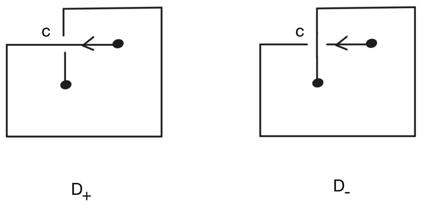
It remains to show that the degree is not zero. The two diagrams in Figure 1 differ only by switching the crossing c.

A direct computation using the affine index labeling rule and the endpoint winding pairs gives

$$P_{D_{+}}(x,y,z)=xy-1,P_{D_{-}}(x,y,z)=1-xy.$$

Therefore,

$$P^{\left(1\right)}\left(D\right)=P_{D_{+}}(x,y,z)-P_{D_{-}}(x,y,z)=2(xy-1)\ne 0.$$

The polynomial is not of degree zero. Hence, $P_D(x,y,z)$ is a Vassiliev invariant of degree one. □

The degree one property is a statement about sensitivity to the resolution of a single singular crossing. The invariant can detect such a resolution when the contribution determined by the winding pair and the affine index is nonzero, but it does not record interactions involving two or more singular crossings. Thus, $P_D(x,y,z)$ is a refinement defined at individual crossings and of Vassiliev degree one rather than a construction that detects interactions among several singular crossings.

5. Metric Bounds

Definition 11 

(Nonconstant coefficient norm). For

$$F(x,y,z)=\sum _{(i,j,k)\in Z^3}{a}_{ijk}{x}^i{y}^j{z}^k,$$

define

$${\parallel F\parallel }_{\ast }=\sum _{(i,j,k)\ne (0,0,0)}\left|a_{ijk}\right|.$$

Definition 12 

(Crossing numbers). The crossing number of a diagram D is $cr\left(D\right)=\#C\left(D\right)$. The crossing number of a planar knotoid K, denoted by $cr\left(K\right)$, is the minimum of $cr\left(D\right)$ over all diagrams D representing K.

Define the winding index essential crossing number of D by

$$c{r}_{wi}\left(D\right)=\#\{c\in C\left(D\right):(l\left(c\right),h\left(c\right),Ind\left(c\right))\ne (0,0,0)\},$$

and define $c{r}_{wi}\left(K\right)$ by minimizing $c{r}_{wi}\left(D\right)$ over all diagrams of K.

Theorem 3. 

For every oriented planar knotoid K,

$$cr\left(K\right)\ge c{r}_{wi}\left(K\right)\ge {\parallel P_K(x,y,z)\parallel }_{\ast }.$$

In particular,

$$cr\left(K\right)\ge \parallel P_K{(x,y,z)\parallel }_{\ast }.$$

Proof. 

Let D be a diagram of K, and write

$$P_D(x,y,z)=\sum a_{ijk}{x}^i{y}^j{z}^k.$$

For $(i,j,k)\ne (0,0,0)$, the coefficient $a_{ijk}$ is the signed sum of the crossings whose triple $(l,h,Ind)$ is $(i,j,k)$. Hence, $|a_{ijk}|$ is bounded above by the number of such crossings. Summing over all nonzero triples gives

$$\parallel P_D{\parallel }_{\ast } \le c{r}_{wi}\left(D\right).$$

Since $P_D=P_K$ for any diagram D of K, taking the minimum over all diagrams gives

$$\parallel P_K{(x,y,z)\parallel }_{\ast }\le c{r}_{wi}\left(K\right).$$

The inequality $c{r}_{wi}\left(K\right)\le cr\left(K\right)$ is immediate from the definitions. □

The inequalities in Theorem 3 are computable lower bounds, not formulas that are always sharp. They are strongest when many crossings have nonzero triples $\left(l\right(c),h(c),Ind(c\left)\right)$ and when little cancellation occurs among crossings with the same triple. They may be weak or may vanish when all nonconstant contributions cancel or when every relevant crossing has triple $(0,0,0)$. The bound is therefore complementary to other estimates and improves a competing numerical bound only when the nonconstant coefficient norm is larger. A sharp example is given after the computations in Section 6.

No universal dominance over previously known crossing number estimates is asserted because the available bounds measure different diagrammatic data. Their numerical strength must be compared on a case-by-case basis. The example in Section 6 proves that the present crossing number bound is sharp for one of the displayed knotoids, but it does not imply that the bound is always sharper than other estimates.

Definition 13 

(Gordian distance and unknotting number). A crossing change is the operation of switching the over/under information at one classical crossing. The Gordian distance $d_G(K,K^{\prime })$ between two oriented planar knotoids is the minimum number of crossing changes required to transform a diagram of K into a diagram of $K^{\prime }$, allowing planar knotoid isotopies before, after and between crossing changes. If no such finite sequence exists, we set $d_G(K,K^{\prime })=\infty$. The unknotting number of K is $u\left(K\right)=d_G(K,O)$, where O is the trivial planar knotoid.

Lemma 2. 

If $D^{\prime }$ is obtained from D by one crossing change, then

$$\parallel P_{D^{\prime }}(x,y,z)-P_D{(x,y,z)\parallel }_{\ast }\le 2.$$

Proof. 

Let c be the changed crossing. A crossing change reverses the sign of c and leaves the underlying flat diagram and the crossing lobe fixed. Thus, the winding pair of c is unchanged. With the convention of Definition 5, the affine index weight of the changed crossing is replaced by its negative. All other crossings have unchanged triples. Hence, the nonconstant part of $P_{D^{\prime }}(x,y,z)-P_D(x,y,z)$ is either zero, or it consists of at most two monomial terms whose coefficients have total absolute value at most 2. Hence, a single crossing change changes the polynomial by norm of at most 2. □

Theorem 4. 

For any oriented planar knotoids K and $K^{\prime }$,

$$d_G(K,K^{\prime })\ge ⌈{\displaystyle \frac{1}{2}}{\parallel P_K(x,y,z)-P_{K^{\prime }}(x,y,z)\parallel }_{\ast }⌉.$$

Consequently,

$$u\left(K\right)\ge ⌈{\displaystyle \frac{1}{2}}{\parallel P_K(x,y,z)\parallel }_{\ast }⌉.$$

Proof. 

If $d_G(K,K^{\prime })=\infty$, the inequality is immediate. Suppose $d_G(K,K^{\prime })=m<\infty$. Choose diagrams

$$D_0,D_1,\dots ,D_m$$

such that $D_0$ represents K, $D_m$ represents $K^{\prime }$, and each step is one crossing change together with planar knotoid isotopies. Since $P_D$ is invariant under planar knotoid isotopy, Lemma 2 and the triangle inequality give

$$\parallel P_K-P_{K^{\prime }}{\parallel }_{\ast } \le {\displaystyle \sum _{r=1}^m}{\parallel P_{D_r}-P_{D_{r-1}}\parallel }_{\ast }\le 2m.$$

Taking the minimum over all such sequences gives the stated Gordian distance bound. The unknotting number bound follows by setting $K^{\prime }=O$ and using $P_O=0$. □

The bounds for Gordian distance and unknotting number are subject to the same limitations. A single crossing change alters the nonconstant coefficient norm by at most two, so the estimates are effective when the polynomial difference is large. We do not claim that these bounds are sharp in general, and they do not replace geometric or diagrammatic estimates. They provide additional obstructions when the data recorded at individual crossings survive cancellation.

6. Comparison with the Winding Signed Sum Polynomial

Bataineh, Batayneh and Alkasasbeh [14] defined the winding signed sum polynomial of a planar knotoid diagram D by

$${\beta }_D(u,v)=\sum _{\lambda \left(c\right)\ne (0,0)}sgn\left(c\right)\left(u^{l\left(c\right)}+v^{h\left(c\right)}\right),$$

(3)

where $\lambda \left(c\right)=\left(l\right(c),h(c\left)\right)$. This invariant records the marginal signed contributions of the leg and head winding numbers. The comparison below explains how the present polynomial fits into this development of knotoid invariants. The invariant $P_D(x,y,z)$ retains the two endpoint winding numbers together with the affine index weight at the same crossing. Consequently, it determines the winding signed sum polynomial after specialization, while the reverse implication may fail because the marginal sums do not remember how the two winding coordinates and the affine index coordinate were paired at individual crossings.

Proposition 3. 

Let ${\left[F\right]}_{0,0}$ denote the coefficient of $x^0{y}^0$ in a Laurent polynomial $F(x,y)$. Then,

$${\beta }_D(u,v)=P_D(u,1,1)+P_D(1,v,1)-2{\left[P_D(x,y,1)\right]}_{0,0}.$$

Moreover, if

$$A_D\left(t\right)=\sum _{c\in C\left(D\right)}sgn\left(c\right)\left(t^{Ind\left(c\right)}-1\right)$$

is the affine index polynomial in the convention used here, then

$$A_D\left(t\right)=P_D(1,1,t).$$

Therefore, $P_D(x,y,z)$ determines both ${\beta }_D(u,v)$ and $A_D\left(t\right)$.

Proof. 

At $z=1$, we have

$$P_D(u,1,1)=\sum _{c\in C\left(D\right)}sg{n}_D\left(c\right)(u^{l_D\left(c\right)}-1),P_D(1,v,1)=\sum _{c\in C\left(D\right)}sg{n}_D\left(c\right)(v^{h_D\left(c\right)}-1).$$

A crossing with $\lambda \left(c\right)=(0,0)$ contributes zero to both sums. For crossings with $\lambda \left(c\right)\ne (0,0)$, the constant term of $P_D(x,y,1)$ is

$$-{\left[P_D(x,y,1)\right]}_{0,0}=\sum _{\lambda \left(c\right)\ne (0,0)}sgn\left(c\right).$$

Rearranging gives exactly (3). The identity $A_D\left(t\right)=P_D(1,1,t)$ follows directly from Definition 6. □

An Explicit Separating Pair

The following computation gives a pair of planar knotoid diagrams that have the same winding signed sum polynomial and the same affine index polynomial but different index refined winding pair polynomials. Thus, in this example, even the ordered pair of the two earlier invariants does not determine the new invariant. The calculation uses only the crossing data displayed in

Table 1. Crossing data for $D_1$.

Crossing	$\mathit{sgn}$	$(\mathit{l},\mathit{h})$	$\mathit{Ind}$
a	$+1$	$(0,0)$	0
b	$+1$	$(1,0)$	$-1$
c	$-1$	$(1,1)$	0
d	$-1$	$(1,1)$	0
e	$+1$	$(1,0)$	1
f	$+1$	$(0,1)$	$-1$
g	$+1$	$(0,1)$	1

and

Table 2. Crossing data for $D_2$.

Crossing	$\mathit{sgn}$	$(\mathit{l},\mathit{h})$	$\mathit{Ind}$
p	$+1$	$(-1,0)$	$-1$
q	$+1$	$(-1,0)$	1
r	$-1$	$(-1,-1)$	0
s	$-1$	$(-1,-1)$	0
t	$+1$	$(0,-1)$	$-1$
w	$+1$	$(0,-1)$	1

.

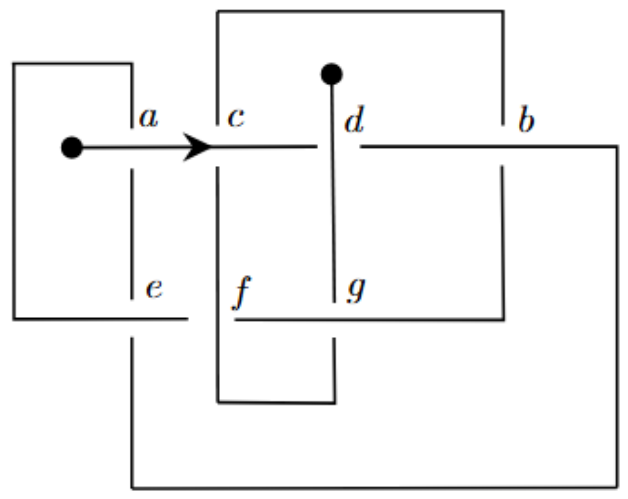
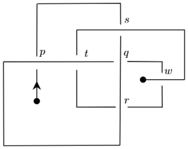
Let $D_1$ be the planar knotoid diagram with seven crossings in Figure 2, with crossings labeled $a,b,c,d,e,f,g$, and let $D_2$ be the planar knotoid diagram with six crossings in Figure 3, with crossings labeled $p,q,r,s,t,w$.

The crossing data computed from the diagrams are listed in Table 1 and Table 2. The affine index weights are obtained from the standard affine labeling of the underlying flat knotoid diagram.

Using Table 1, we obtain

$$\begin{array}{cc}\hfill P_{D_1}(x,y,z)& =(x{z}^{-1}-1)-(xy-1)-(xy-1)\hfill \\ \hfill & +(xz-1)+(y{z}^{-1}-1)+(yz-1)\hfill \\ \hfill & =(x+y)(z+z^{-1})-2-2xy.\hfill \end{array}$$

For $D_2$, Table 2 gives

$$\begin{array}{cc}\hfill P_{D_2}(x,y,z)& =(x^{-1}{z}^{-1}-1)+(x^{-1}z-1)\hfill \\ \hfill & -(x^{-1}{y}^{-1}-1)-(x^{-1}{y}^{-1}-1)\hfill \\ \hfill & +(y^{-1}{z}^{-1}-1)+(y^{-1}z-1)\hfill \\ \hfill & =(x^{-1}+y^{-1})(z+z^{-1})-2-2x^{-1}{y}^{-1}.\hfill \end{array}$$

(4)

Thus

$$P_{D_1}(x,y,z)\ne P_{D_2}(x,y,z).$$

Indeed, the two expressions satisfy

$$P_{D_1}(x,y,z)=xy{P}_{D_2}(x,y,z),$$

but they are distinct Laurent polynomials.

For the winding signed sum polynomial, the crossing with winding pair $(0,0)$ does not contribute. Using Table 1 and Table 2, we obtain

$$\begin{array}{cc}\hfill {\beta }_{D_1}(u,v)& =(u+1)-(u+v)-(u+v)\hfill \\ \hfill & +(u+1)+(1+v)+(1+v)=4,\hfill \end{array}$$

and

$$\begin{array}{cc}\hfill {\beta }_{D_2}(u,v)& =2(u^{-1}+1)-2(u^{-1}+v^{-1})+2(1+v^{-1})=4.\hfill \end{array}$$

Consequently,

$${\beta }_{D_1}(u,v)={\beta }_{D_2}(u,v)=4.$$

For comparison, write the affine index polynomial in the convention used above as

$$A_D\left(t\right)=\sum _{c\in C\left(D\right)}sgn\left(c\right)\left(t^{Ind\left(c\right)}-1\right).$$

The crossings of index zero contribute nothing. For $D_1$ and $D_2$, respectively,

$$\begin{array}{cc}\hfill A_{D_1}\left(t\right)& =2(t^{-1}-1)+2(t-1)=2t+2t^{-1}-4,\hfill \\ \hfill A_{D_2}\left(t\right)& =2(t^{-1}-1)+2(t-1)=2t+2t^{-1}-4.\hfill \end{array}$$

Hence,

$${\beta }_{D_1}={\beta }_{D_2},A_{D_1}=A_{D_2},P_{D_1}\ne P_{D_2}.$$

This pair therefore shows that neither the winding signed sum polynomial nor the affine index polynomial, even when considered together, determines the index refined winding pair polynomial. The marginal winding sums cancel to the same constant, and the affine index distributions are identical, while $P_D(x,y,z)$ retains how the two endpoint winding numbers and the affine index weight are attached at each individual crossing. For this particular pair, the new invariant is more discriminating than the two comparison polynomials.

For this particular pair, the specialization $z=1$ already distinguishes the diagrams:

$$P_{D_1}(x,y,1)=2x+2y-2xy-2$$

and

$$P_{D_2}(x,y,1)=2x^{-1}+2y^{-1}-2x^{-1}{y}^{-1}-2.$$

Thus, this example demonstrates the importance of retaining the joint winding pair rather than merely its marginal sums. It is not, by itself, an example in which the distinction depends exclusively on the affine index variable z.

Accordingly, this pair proves that the ordered pair $({\beta }_D,A_D)$ does not determine $P_D$, while the exact decomposition in Remark 1 explains the independent information carried by z. These are distinct refinement mechanisms and are not conflated here.

Let $K_i$ be the planar knotoid represented by $D_i$. The displayed formulas give

$$\begin{array}{c}\hfill \parallel P_{K_1}{\parallel }_{\ast }={\parallel P_{K_2}\parallel }_{\ast }=6.\end{array}$$

Since $D_2$ has six crossings, Theorem 3 gives $6\le cr\left(K_2\right)\le 6$, and hence, $cr\left(K_2\right)=6$. Thus, the crossing number bound is sharp for $K_2$. Since $D_1$ has seven crossings, the same argument gives $6\le cr\left(K_1\right)\le 7$.

7. Conclusions

We introduced an index refined winding pair polynomial that records, at each crossing of an oriented planar knotoid diagram, the winding numbers of the crossing lobe around the two endpoints together with the affine index weight. The invariant is compatible with the basic knotoid operations considered above, has Vassiliev degree one and yields lower bounds for crossing number, Gordian distance and unknotting number. Proposition 3 shows that it determines both the winding signed sum polynomial and the affine index polynomial. The separating pair in Section 6 shows that the converse fails even when these two earlier invariants are considered together.

The construction also has clear limitations. A crossing contributes zero when $l\left(c\right)$, $h\left(c\right)$ and $Ind\left(c\right)$ are all zero, and crossings with the same triple and opposite signs may cancel. The invariant is therefore not complete. For a diagram with n crossings, a straightforward implementation may traverse a subpath containing order n arcs for each crossing and may require order $n^2$ elementary arc visits; no optimality claim is made for this procedure. The metric bounds are not asserted to be sharp in general. Future work includes finding minimal realized examples in which the distinction depends exclusively on the variable z, comparing the bounds systematically with other estimates on knotoid tables and developing more efficient computational methods.