Differential Evolution Flexible Integrated Assembly Production Distribution Scheduling (DE-FIAPDS)

Abstract

This study addresses the gap in research on distributed integrated scheduling for complex products by presenting a tree-structured framework enhanced with Differential Evolutionary Flexible Integrated Assembly Production Distribution Scheduling (DE-FIAPDS). The algorithm’s effectiveness is demonstrated by validating standard benchmark problems and custom-generated test cases. Using Taguchi’s method and comparative analysis, we developed GA and DE heuristic evolutionary algorithms for the scheduling problem. Over the course of 30 independent replications, applied to 100 randomly generated instances, the DE-FIAPDS algorithm was observed to produce an average final-generation makespan. We calculate the time complexity of the basic DE by combining these additional steps with the basic DE time complexity, such as forward conversion, backward conversion and local search, which can be expressed as $O(G_{\max }·N_{\mathrm{pop}}·(d+n_{\mathrm{op}}log{n}_{\mathrm{op}}))$, where $G_{\max }$ is the maximum number of generations, $N_{\mathrm{pop}}$ is the number of individuals in the given population, d is the dimension of the problem, and $n_{\mathrm{op}}$ is the the number of operations in FIAPDS. The proposed DE-FIAPDS gives the same results as GA-FIAPDS, although in some instances they differ by a huge difference in makespan. On the other hand, its computing time was 100 times quicker.

1. Introduction

Efficient scheduling is crucial in today’s manufacturing industry to minimize production costs, maximize resource utilization, and improve overall production effectiveness. According to Pinedo [1], scheduling problems often arise when there is a mismatch between effective utilization of manufacturing resources and optimization of production goals and cost efficiency. The scheduling problem is strongly Non-deterministic Polynomial (NP-hard), which means that it is at least as difficult as the hardest problems in the class of Non-deterministic Polynomial, for which no known polynomial-time algorithm can provide an exact solution [2].

Traditionally, in many scheduling problems, to produce items on several machines, they need to be scheduled independently. Specifically, in the integrated scheduling problems, we built all components from the given times using a tree-like structure. In this kind of structure, they processed the leaves on the tree first before the items were assembled into a specific component according to a hierarchical assembly structure. Moreover, integrated scheduling problems are divided into two main stages: processing and assembly. These two stages tend to lengthen the manufacturing cycles, increase production costs, and also increase processing time.

Destouet et al. [3] carried out survey research on scheduling that aligns with the transition from Industry 4.0 to Industry 5.0, following advancements in AI, IoT, and optimization concepts, divided into research problems. Mraihi et al. [4] reviewed modern manufacturing, adding to the busy machines and ineffective prioritization problem. The study by Wang et al. [5] involves systematically arranging production tasks in line with pre-set plans and market requirements. Ardyanti et al. [6] classified research about Integrated Scheduling Problems (ISPs), such as Planning Scheduling [7,8,9], ISP for Manufacturing [10,11,12,13,14,15,16], Production and Distribution [17,18,19,20,21], Assembly Job Shop Scheduling [22,23,24,25], Control and Robotics [26], Supply Chain [27], Logistics [28,29], Security Systems [30], Energy and Carbon [31,32], and Health [33,34,35,36].

Although the ISP extends job shop scheduling problems, the present study focuses on a scheduling optimization problem in flexible machine and multi-factory environments. The proposed approach employs a remaining-work probability selection coding strategy to minimize the maximum product manufacturing completion time. As described by Xie et al. [37], the integrated scheduling problem (ISP) approach, also known as the flexible integrated scheduling problem (FISP), uses the Artificial Bee Colony Algorithm. Gao et al. [38,39] represented process constraints using tree-structured relationships. Yuan et al. [40] proposed a three-chain method for complex product manufacturing with priority constraints on flexible machines and flexible factories. To ensure the feasibility, quality, and heterogeneity of the initial population, an encoding strategy grounded in a remaining-work probability selection mechanism is proposed. In addition, two dedicated methods are developed for the crossover and mutation operators to handle specific cases of forward and backward conversion of flexible machines and factories, each ensuring the correctness and admissibility of the offspring chromosomes produced. To further strengthen the algorithm’s search performance, a machine-oriented search strategy is introduced. In addition, a straightforward and practical decoding procedure is provided. The feasibility and effectiveness of the proposed algorithm are confirmed through comprehensive experimental evaluation. This section specifically examines production allocation among up to five factories, with the Differential Evolution Algorithm adopted as the underlying optimization technique, having been established as the superior method at the IEEE World CEC 2025 (https://attend.ieee.org/wcci-2026/ieee-cec-2025/ accessed on 3 April 2026), and used Python Numba for fast machine code (http://numba.pydata.org/ accessed on 3 April 2026) [41,42,43].

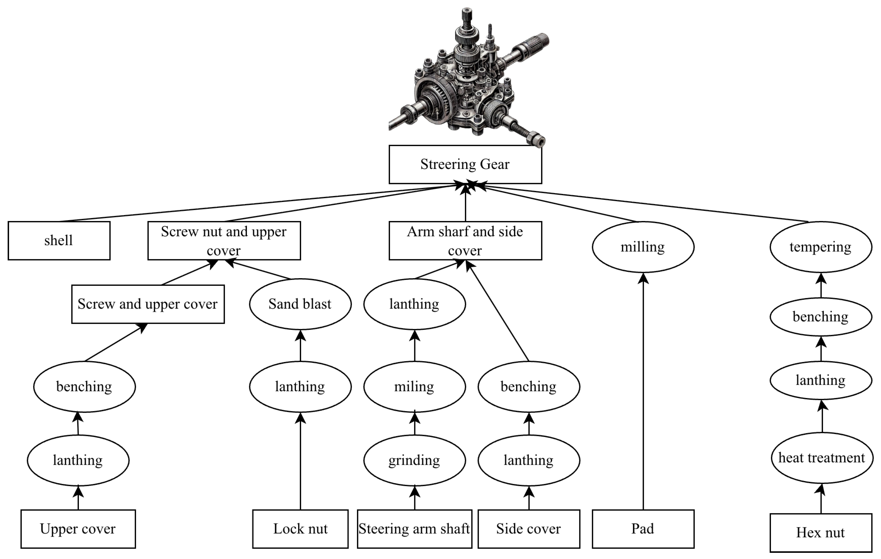
The organizational structure of this paper is delineated as follows. Section 2 is rigorously formulated for the Integrated Scheduling Problem (ISP). For this research, we considered complex products, flexible machines and factories, as shown in in Figure 1. From Figure 1, our framework is a tree-structured framework where every node and leaf node describes an assembly process performed under flexible machine and factory settings. Then, Section 3 is about basic Differential Evolutionary (DE). Section 4 systematically describes Differential Evolutionary Flexible Integrated Assembly Production Distribution Scheduling (DE-FIAPDS), comprising the encoding mechanism grounded in remaining work quantities, two independent crossovers, selection with a local search strategy, the associated decoding procedure, and mutation operators based on forward and backward conversion strategies to maintain consistency with Differential Evolution (DE). Section 5 is the experimental setup of two comparative studies designed to rigorously evaluate algorithm performance. Section 6 presents the results. Section 7 synthesizes the summary and suggests avenues for future investigation.

2. Problem Formulation

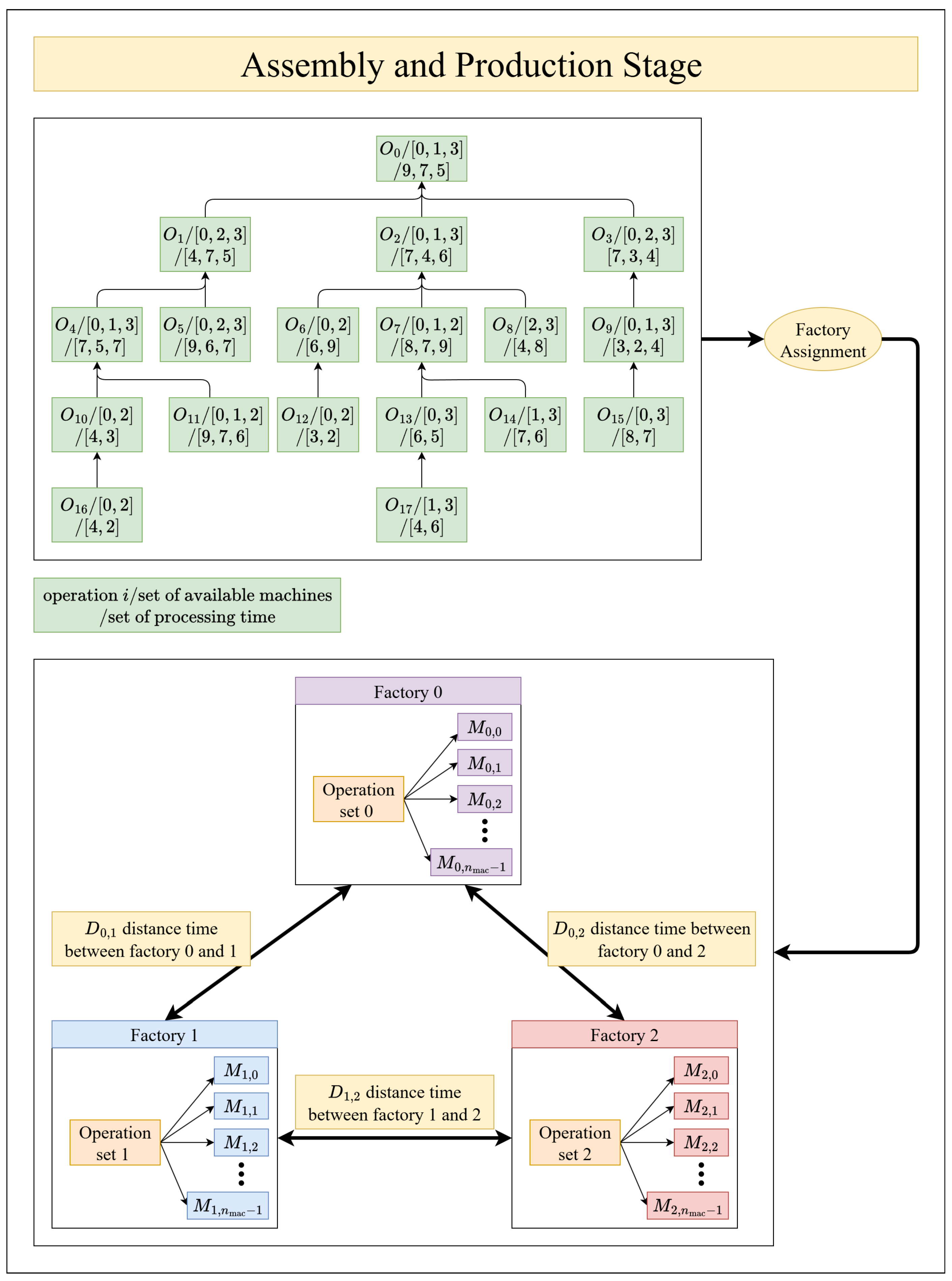
As shown in Figure 2, consider $n_{\mathrm{op}}$ operations from a tree-structured complex product, the manufacturing workload of which is collaboratively distributed across $n_{\mathrm{fac}}$ factories, or equivalently, processing centers. Without loss of generality, each factory is assumed to house a uniform number of machines, denoted by $n_{\mathrm{mac}}$. To formally govern the admissible processing sequences among the constituent operations, a priority constraint set $\mathcal{C}$ is defined to be $\mathcal{C}=\{(O_i,O_j)\mid O_i,O_j\in \mathcal{O}\}$, where the set $\mathcal{O}$ is the set of all operations $O_i$. If $(O_i,O_j)\in \mathcal{C}$, operation $O_i$ is the immediate predecessor of $O_j$, which means that $O_i$ must be finished before operation $O_j$ is processed. For each operation $O_i$, define two variables that represent starting time $s_i$ and completion time $c_i$. When the operation $O_i$ is processed in factory f at machine m, we define $x_{imf}$ and set it to 1, otherwise 0. The subscript sequence of $x_{imf}$ follows the convention that we first need to place the operation at an available machine in any factory. For each immediate predecessor of $O_j$ that has the same machine and factory placement at $O_j$, we define the variable $y_{ij}$, where $O_i$ is one of the immediate predecessor operations. If we set $y_{ij}=1$, it means $O_j$ is proccessed after $O_i$; otherwise, we set $y_{ij}=0$. The factory set F is defined as $F=\{f\mid f\in \{0,1,2,\dots ,n_{\mathrm{fac}}-1\}\}$, and the machine set M is defined as $M=\{m\mid m\in \{0,1,2,\dots ,n_{\mathrm{mac}}-1\}\}$. Because not all machines are available to all operations, we define the set of available machines $A{M}_i$ for each operation $O_i$. We also assume that the set of all machines M can be found in any factory. We also define $p_{im}$ as the processing duration required for operation $O_i$ on machine m. The distance from the first factory to the second factory $f_a$ and $f_b$ is defined as $D_{f_a,f_b}$. We also define $z_{ij}$, which has the same characteristic as $y_{ij}$, but it is specified to include the traversing time when bringing all the products after processing all immediate predecessors $O_i$ of the operation $O_j$ to the factory where $O_j$ is placed. The scheduling objective is to minimize the total completion time of the product. Accordingly, the problem investigated in this study is formally formulated as follows.

$$\begin{array}{cc}\hfill & \mathrm{minimize}{C}_{\max }=\underset{i}{max}\left(c_i\right)\hfill \end{array}$$

(1)

$$\begin{array}{cc}\hfill & \mathrm{subject}\mathrm{to}\hfill \end{array}$$

$$\begin{array}{cc}\hfill & \sum _{f\in F}\sum _{m\in A{M}_i}{x}_{imf}=1,i=0,\dots ,n_{\mathrm{op}}-1\hfill \end{array}$$

(2)

$$\begin{array}{cc}\hfill & p_i=\sum _{f\in F}\sum _{m\in A{M}_i}{x}_{imf}{p}_{im},i=0,\dots ,n_{\mathrm{op}}-1\hfill \end{array}$$

(3)

$$\begin{array}{cc}\hfill & s_i\ge \underset{\left\{j\right|(O_j,O_i)\in \mathcal{C}\}}{max}\left(c_j+z_{ji}{D}_{f_j,f_i}\right),i=0,\dots ,n_{\mathrm{op}}-1\hfill \end{array}$$

(4)

$$\begin{array}{cc}\hfill & c_i=s_i+p_i,i=0,\dots ,n_{\mathrm{op}}-1\hfill \end{array}$$

(5)

$$\begin{array}{cc}\hfill & y_{ij}+y_{ji}\ge x_{imf}+x_{jmf}-1,\left(i,j=0,\dots ,n_{\mathrm{op}}-1\right)\wedge \left(i\ne j\right)\wedge \left(m\in A{M}_i\cap A{M}_j\right)\wedge \left(f\in F\right)\hfill \end{array}$$

(6)

$$\begin{array}{cc}\hfill & s_j\ge s_i+p_i-(1-y_{ij})L+z_{ij}{D}_{f_i,f_j},\left(i,j=0,\dots ,n_{\mathrm{op}}-1\right)\wedge \left(i\ne j\right)\hfill \end{array}$$

(7)

$$\begin{array}{cc}\hfill & s_i\ge 0,i=0,\dots ,n_{\mathrm{op}}-1\hfill \end{array}$$

(8)

In the above problem, $c_i$ is the completion time defined by operation $O_i$. $C_{\max }$ is the maximum of all possible $c_i$. In constraint Equation (2), we set every operation only in one factory and one available machine. As shown in Equation (3), $p_i$ is processing time in operation $O_i$ after we have assigned that operation to a specific machine and factory. We set the constraint for the starting time of each operation, where its starting time must be initiated after all its immediate predecessors have been completed, as shown in Equation (4). The variable $D_{f_i,f_j}$ is the distance (in unit time) for bringing the product after operation $O_i$ from factory $f_i$ to be processed by operation $O_j$ in factory $f_j$. In Equation (5), we have to make sure that $c_i$ satisfies the total processing time for its operation, where the starting time is $s_i$. The constraint in Equation (6) is a constraint to avoid any overlap between two operations $O_i$ and $O_j$ for any operation $O_i$ that is an immediate predecessor of $O_j$ at machine m and factory f. The constraint in Equation (7) is a constraint that the starting time for any operation $O_j$ that is not an immediate predecessor of $O_i$ can be started earlier than $O_i$ by setting a specific large constant L. Based on the last constraint in Equation (8), we have to make sure that the starting point is never negative. Every operation has an opportunity to start.

For realistic conditions, we need to define the following assumptions:

1.

Operations must not be interrupted while processing on the equipment. Once the operation commences, it cannot be halted until its completion.

2.

Every machine only processes one operator at a time.

3.

Any operation may be executed on one of the accessible machines.

4.

A prior tight-predecessor on the same machine is preferred.

5.

Preceding predecessors are favored for allocation to the machine and factory. For any operation, it cannot start until all its predecessors are finished.

6.

No loss of equipment. This presumes that no equipment will sustain damage or require repair throughout the execution of all procedures.

7.

No loss of time. We disregard the temporal expenses associated with component supply and equipment initialization, meaning that the release time for each step is zero.

8.

Prior information knowledge about the processing time in each operation. We know prior to the execution of the procedure the equipment required and the necessary processing duration.

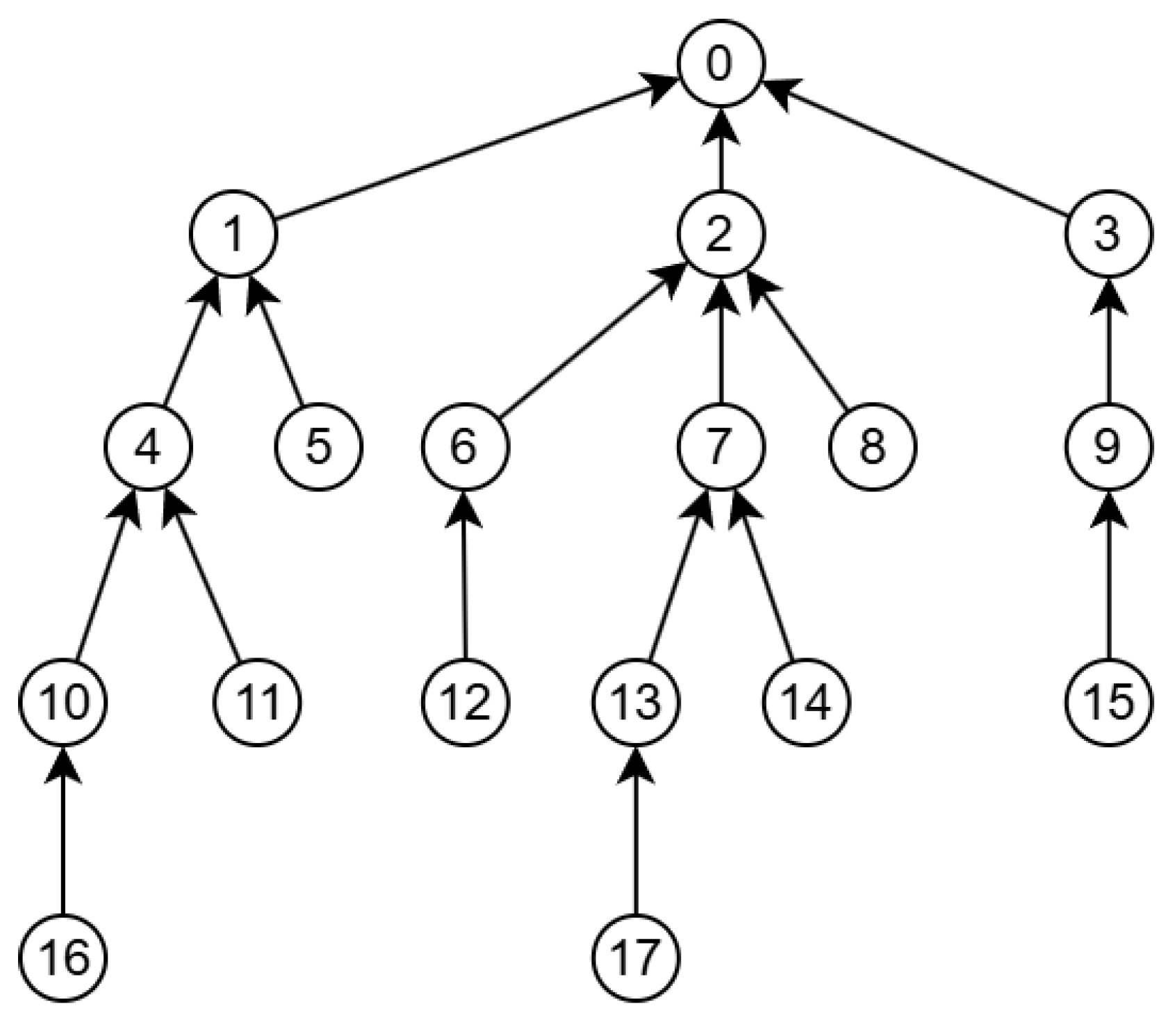
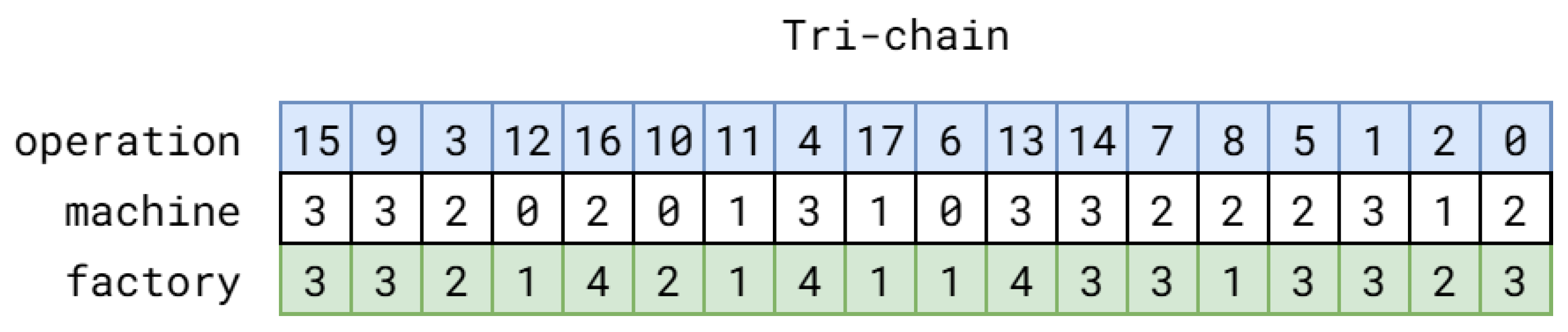
For example, here we present the input data for 18 assembly operations in a tree-like structure in Figure 3 that will be assigned to up to four machines and five different factories. In that case, we also show the one possible solution to our problem using a tri-chain encoding in Figure 4. To store the tree-like structure of the hierarchical assembly operation, we use a simple array that stores the successors of each operation as in

Table 1. Representing the number of immediate predecessors for each operation $O_j$ in the tree-like structure. The root operation $O_0$ has no immediate predecessor, so we set it to negative one.

$O_j$	0	1	2	3	4	5	6	7	8	9	10	11	12	13	14	15	16	17
${\mathrm{Tree}}_{\mathrm{op}}$	$-1$	0	0	0	1	1	2	2	2	3	4	4	6	7	7	9	10	13

.

In the above example, we also need to know the available machines of each operation, which have been collected in

Table 2. (a) An example of machine assignment for 18 assembly operations. The processing time number for operation $p_{im}$ for $O_i$ and machine m. There are some machines that have no processing time, which represents an unavailable machine for the given operation. (b) An example of transfer time between two factories. These travel times are symmetric (Factory 1 to Factory 2 is the same as Factory 2 to Factory 1).

(a)
Operation	$\mathit{m}=\mathbf{0}$	$\mathit{m}=\mathbf{1}$	$\mathit{m}=\mathbf{2}$	$\mathit{m}=\mathbf{3}$
$O_0$	9	7	-	5
$O_1$	4	-	7	5
$O_2$	7	4	-	6
$O_3$	7	-	3	4
$O_4$	7	5	-	7
$O_5$	9	-	6	7
$O_6$	6	-	9	-
$O_7$	8	7	9	-
$O_8$	-	-	4	8
$O_9$	3	2	-	4
$O_{10}$	4	-	3	-
$O_{11}$	9	7	6	-
$O_{12}$	3	-	2	-
$O_{13}$	6	-	-	5
$O_{14}$	-	7	-	6
$O_{15}$	8	-	-	7
$O_{16}$	4	-	2	-
$O_{17}$	-	4	-	6
(b)
Start Factory		End Factory	Time
1		0	1
2		0	2
2		1	1
3		0	1
3		1	3
3		2	2
4		0	2
4		1	1
4		2	1
4		3	2

. We assume that all factories have the same type of machines. It means that for each operation and its corresponding available machines, we can put that operation in any factory. The more complicated problem can be handled by restricting these to available factories for each machine. We leave this to our future work.

3. Basic DE

For this section, we follow the description of DE from [44]. Essentially, DE modifies the real-valued vector taken as a sample in a way that differs from the other two random vectors. After that, it performs another vector manipulation and checks if the vectors will have the minimum value. Before we can start DE, we need to determine the control parameters. The parameters comprise the mutation scale factor ($F_{\mathrm{scale}}$), population size ($N_{\mathrm{pop}}$), and the crossover probability ($C_r$). Identifying an effective parameter configuration enhances the algorithm’s capability to converge toward the global optimum or a near-optimal region at an accelerated rate.

We represent the subsequent generations in DE as $g=0,1,\dots ,G_{max}$. In the current population generation, the i-th vector is expressed as:

$${\mathbf{X}}_{i,g}={\left[x_{1,i,g},x_{2,i,g},\dots ,x_{d,i,g}\right]}^T$$

(9)

where d is a vector dimension. The first population ($g=0$) of vectors is often created randomly to maximize coverage of the confined search space. Consequently, the j-th element of the i-th vector can be represented as

$$x_{j,i,0}=x_{j,\min }+\left(x_{j,\max }-x_{j,\min }\right)U(0,1)$$

(10)

where a random variable $U(0,1)$ represents a real number distributed uniformly between 0 and 1. The lower and upper bounds $(x_{j,\min },x_{j,\max })$ are determined by the problems. After we initialize the initial population ${\mathbf{X}}_{i,g}$, we can use these vectors to perform mutation.

3.1. Mutation Basic DE

During the evolutionary process, a perturbation that is applied to an individual might be considered to be part of the mutation. A candidate vector that is drawn from the current generation is identified as the target vector in the DE. An example of a mutant vector is produced by the mutation operator. ${\mathbf{V}}_{i,g}={[v_{1,i,g},v_{2,i,g},\dots ,v_{d,i,g}]}^T$. It is widely recognized that various mutation strategies are available for the DE. This work adheres to the DE/best/1. The term “best” means that we select the best individuals from the population after we perform mutation on all individuals. The last term “1” means that we use only one difference to update a vector. This update can be written explicitly as

$${\mathbf{V}}_{i,g}={\mathbf{X}}_{\mathrm{best},g}+F_{\mathrm{scale}}\left({\mathbf{X}}_{r_1,g}-{\mathbf{X}}_{r_2,g}\right)$$

(11)

In the above update, we define $r_1$ and $r_2$ as two unique random integers drawn from $\{1,2,\dots ,N_{\mathrm{pop}}\}$ for each individual in each generation. The individual vector ${\mathbf{X}}_{\mathrm{best},g}$ represents the vector that, within the population at the time of generation g, achieves the highest fitness value (that is, the value of the minimum objective function in the context of a minimization issue). The scaling factor $F_{\mathrm{scale}}$ is a real-valued constant defined over the interval [0, 2], typically taking a value less than 1. The mutation operator in DE differs substantially from that employed in classical GA. In contrast to the marginal perturbations characteristic of GA mutation, DE mutation is performed through a linear combination of individual vectors. Upon completing the mutation operation for each individual vector, the crossover operation is subsequently applied.

3.2. Crossover Basic DE

The crossover illustrates a standard instance of information sharing among individuals. The crossover operator vector ${\mathbf{U}}_{i,g}={[u_{1,i,g},u_{2,i,g},\dots ,u_{d,i,g}]}^T$, by mixing components from ${\mathbf{X}}_{i,g}$ and its associated ${\mathbf{V}}_{i,g}$ mutated vector. The formulation to perform crossover is conceived by these conditional transformations:

$$u_{j,i,g}=\left\{\begin{array}{cc}{v}_{j,i,g},\hfill & \mathrm{if}U(0,1)\le C_r\mathrm{or}j=q\hfill \\ x_{j,i,g},\hfill & \mathrm{otherwise}\hfill \end{array}\right.$$

(12)

where $j=q$. We are able to use an integer that has been chosen at random from within the interval from $[1,d]$, ensuring ${\mathbf{U}}_{i,g}$ inherits a minimum of one element from the altered vector ${\mathbf{V}}_{i,g}$. The real-valued constant defined over the interval $[0,1]$ has a crossover probability $C_r$.

3.3. Selection Basic DE

The selection of the operator is the fundamental task of determining if the vector ${\mathbf{U}}_{i,G}$ substitutes the existing individual in the future generation, which can be expressed as:

$${\mathbf{X}}_{i,g+1}=\left\{\begin{array}{cc}{\mathbf{U}}_{i,g},\hfill & \mathrm{if}f\left({\mathbf{U}}_{i,g}\right)\le f\left({\mathbf{X}}_{i,g}\right)\hfill \\ {\mathbf{X}}_{i,g},\hfill & \mathrm{otherwise}\hfill \end{array}\right.$$

(13)

In this context, $f\left(\mathbf{X}\right)$ denotes the objective function, where f operates on a designated vector $\mathbf{X}$. In the aforementioned equation, we advance the individual vector ${\mathbf{X}}_{i,g}$ if the newly generated vector ${\mathbf{U}}_{i,g}$ demonstrates a superior minimum compared to the minimum of the objective function associated with ${\mathbf{X}}_{i,g}$. These procedures of mutation, crossover, and selection are repeated until we have convergent solution vector ${\mathbf{X}}_{i,g}$.

4. DE for FIAPDS

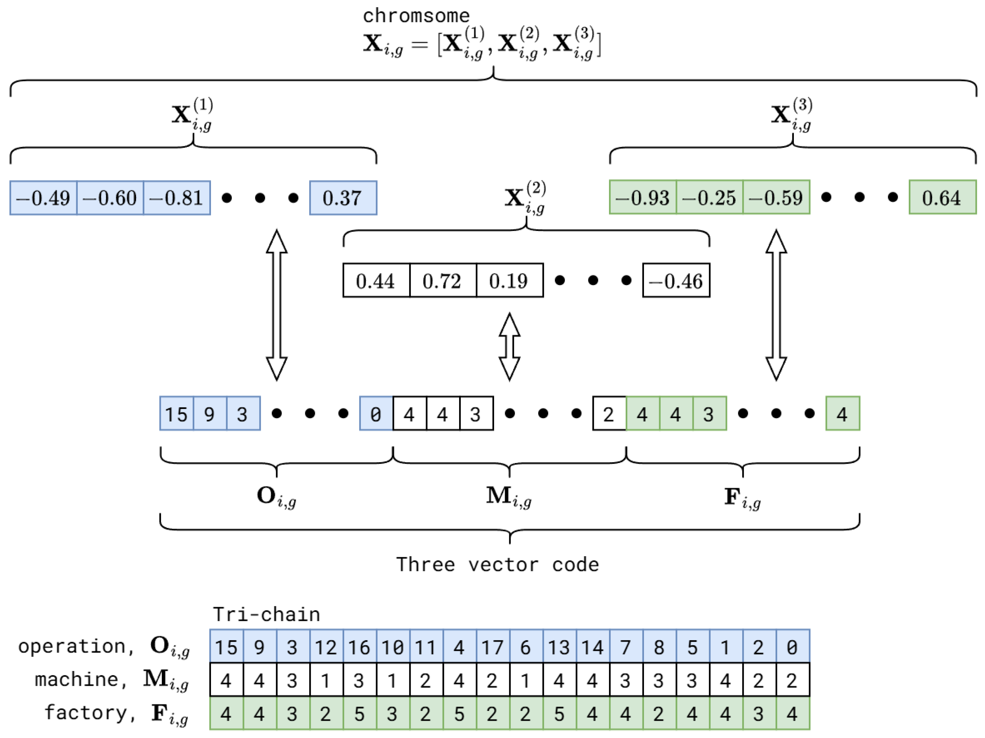
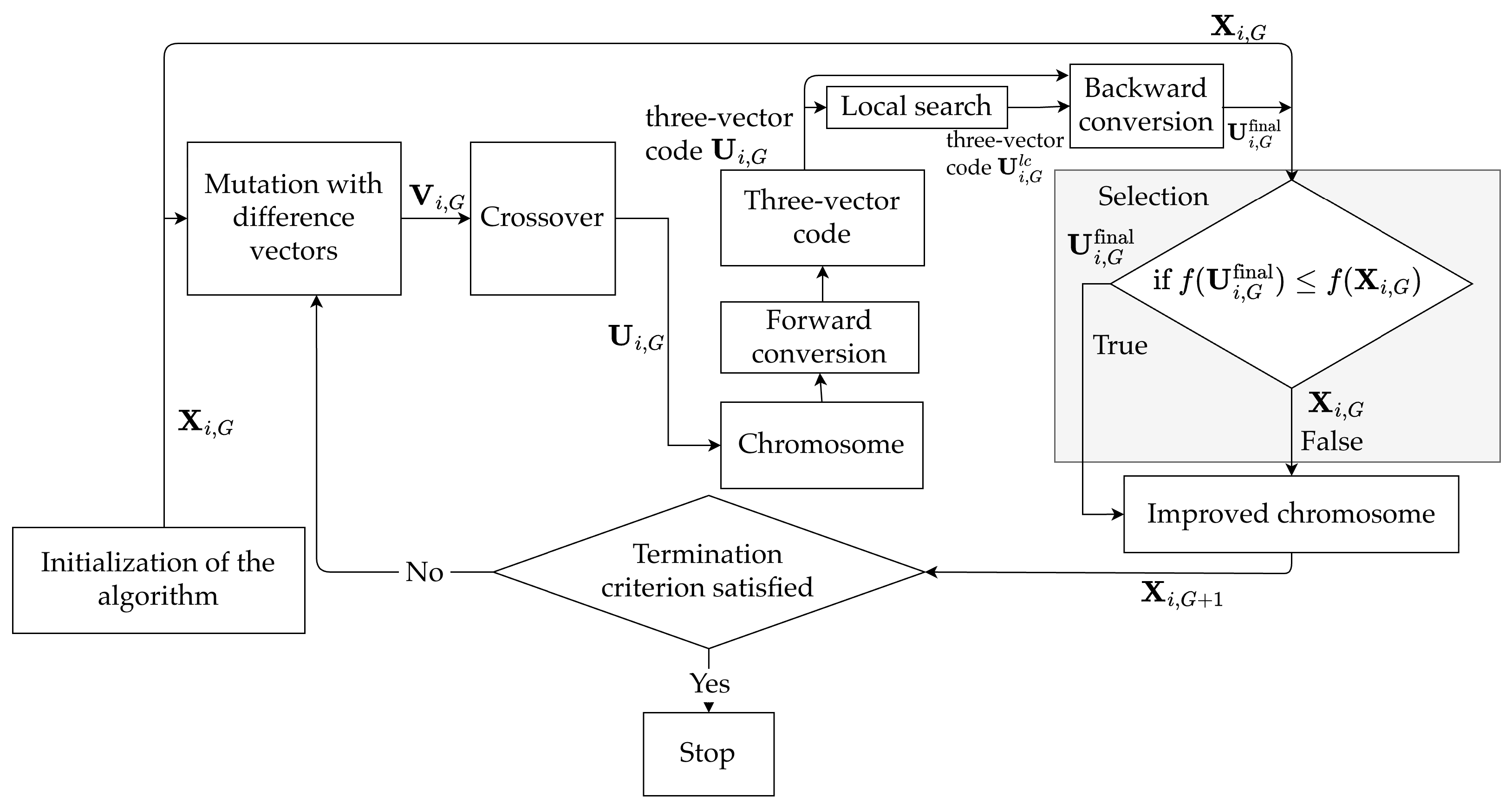
We apply DE to our problem FIAPDS; we call it DE-FIAPDS. This algorithm was developed from  [40]. We use the principle of DE in the new problem and also develop the new local search. Our local search is simpler to implement than in [40]. To start the DE, we have to prepare the initial real-valued vector ${\mathbf{X}}_{i,g}$, which we call a chromosome. These vectors will be converted back and forth to what is called the “three-vector code”; see Figure 5. Specifically, the proposed DE-FIAPDS can be explained in the following steps (see Figure 6).

First, set up the size of the population or the number of symbols as ($N_{\mathrm{pop}}$), then the ($C_r$) crossover probability, the ($F_{\mathrm{scale}}$) mutation scale factor, and ($G_{\max }$) maximum number of generations. Second, initialize the population and set $g=0$. Third, evaluate each chromosome with the given objective function f, and label the best individual with ${\mathbf{X}}_{best,g}$. Fourth is the mutation phase. We generate $N_{\mathrm{pop}}$ vectors ${\mathbf{V}}_{i,g}$ by employing the mutation operator outlined in Equation (11). Fifth is the crossover phase; generate $N_{\mathrm{pop}}$ vectors ${\mathbf{U}}_{i,g}$, according to the crossover condition transformation given in Equation (12). Sixth is vector ${\mathbf{U}}_{i,g}$ for the local search. The seventh step is the selection phase. Evaluate each of the $N_{\mathrm{pop}}$ to find the best candidate vectors ${\mathbf{X}}_{i,g+1}$, by comparing the objective value of three vector codes ${\mathbf{U}}_{i,g}$ and against that of the current vector ${\mathbf{X}}_{i,g}$, described in Equation (13). Then, add the generation counter by setting $g\leftarrow g+1$. In the eighth step, recalculate these new chromosomes’ ${\mathbf{X}}_{i,g}$’s again to find the ${\mathbf{X}}_{best,g}$. In the ninth step, if $G<G_{max}$, proceed to Step 4; if not, halt the procedure and return ${\mathbf{X}}_{best,g}$.

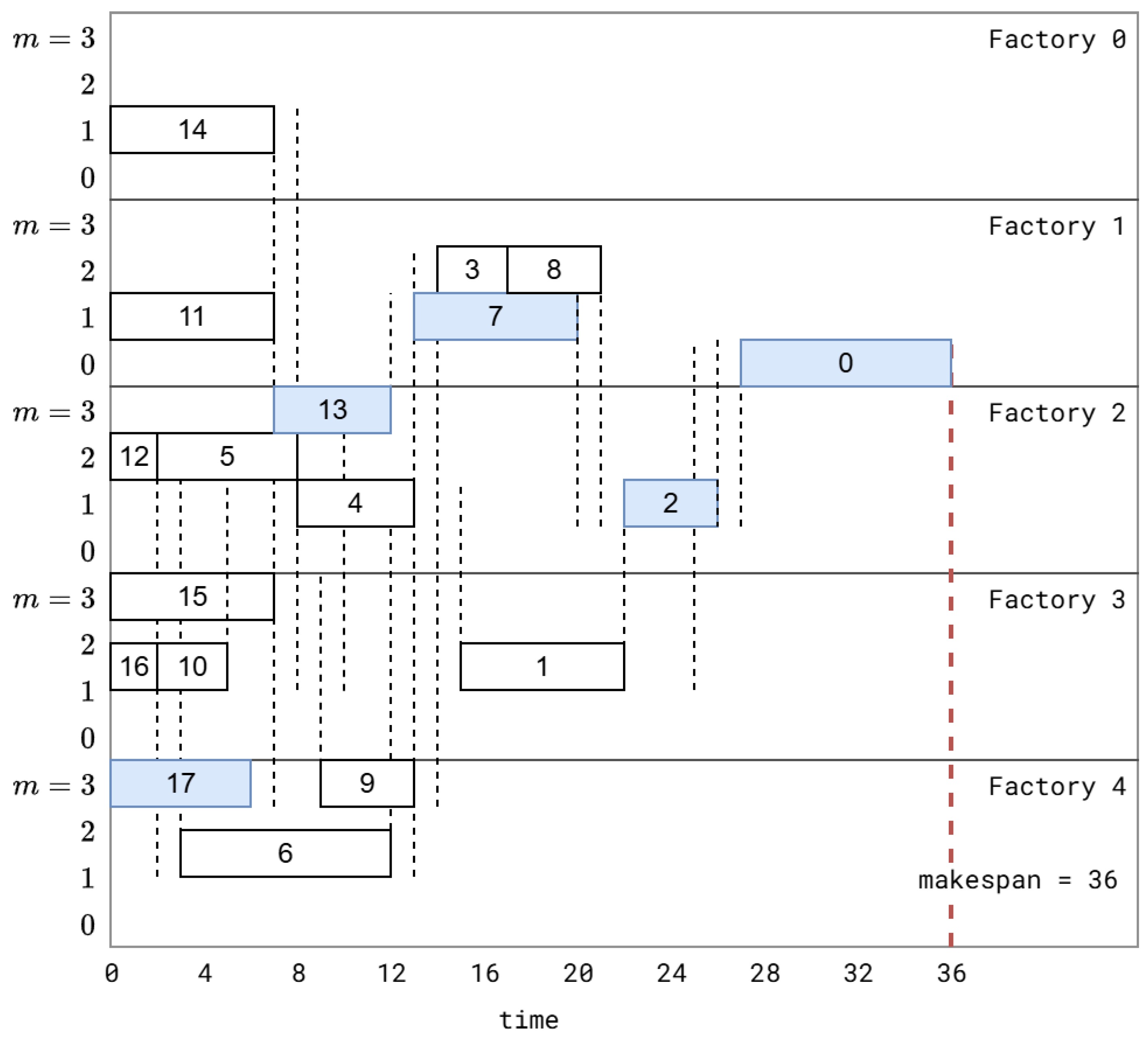
The proposed DE-FIAPDS integrates global exploration via evolutionary mechanisms with local exploitation through a dedicated local search algorithm, where local search is applied to the three-vector code of the chromosome ${\mathbf{U}}_{i,g}$ (or $[{\mathbf{O}}_{i,g},{\mathbf{M}}_{i,g},{\mathbf{F}}_{i,g}]$; see Figure 5) rather than the chromosome ${\mathbf{X}}_{i,g}$. Implementing DE FIAPDS requires addressing two key components: chromosome evaluation and local search application. For evaluation, a real-valued chromosome is first transformed into a discrete three-vector code representation via forward conversion. Read Section 4.3 for further explanation. This three-vector code is then decoded into a stacked Gantt chart of all factories, as shown in Figure 7.

4.1. Initialization of Chromosome

In our proposed DE, each candidate solution i is encoded as a d-dimensional real-valued vector ${\mathbf{X}}_{i,g}={[x_{1,i,g},x_{2,i,g}\dots ,x_{d,i,g}]}^T$ where d is set to $3n_{\mathrm{op}}$ and g is the index for the generation. To simultaneously address sequencing decisions, machine assignment, and factory assignment, ${\mathbf{X}}_{i,g}$ is partitioned into three equal sub-vectors:

• The first segment, ${\mathbf{X}}_{i,g}^{\left(1\right)}={[x_{1,i,g},x_{2,i,g},\dots ,x_{n_{\mathrm{op}},i,g}]}^T$, encodes machine operation sequencing.
• The second segment, ${\mathbf{X}}_{i,g}^{\left(2\right)}={[x_{n_{\mathrm{op}}+1,i,g},x_{n_{\mathrm{op}}+2,i,g},\dots ,x_{2n_{\mathrm{op}},i,g}]}^T$, represents the assignment of all operations to their available machines.
• The last segment ${\mathbf{X}}_{i,g}^{\left(3\right)}=[x_{2n_{\mathrm{op}}+1,i,g},x_{2n_{\mathrm{op}}+2,i,g},\dots ,x_{3n_{\mathrm{op}},i,g}]$ is for the factory assignment.

Similar to the basic DE, each element $x_{j,i,g}$ in the initial population is generated through uniform random sampling. Individual chromosomes are initialized according to Equation (10), with lower and upper bounds set to $x_{j,min}=-\delta$ and $x_{j,max}=\delta$ for all $j=1,2,\dots ,3n_{\mathrm{op}}$.

4.2. Decoding Three-Vector Code

The proposed DE-FIAPDS employs a deterministic decoding mechanism to calculate the three-vector code ${\mathbf{X}}_{i,g}^{\left(\mathrm{three}\text{-}\mathrm{vec}\right)}$ into a feasible schedule. We cannot immediately decode a chromosome represented by real-valued vectors into makespan because the chromosome does not explicitly represent the assignment of operations to machines and factories. Section 4.3 will further elucidate the process of converting that chromosome into its three-vector coding form. Now we want to explain Algorithm 1, which decodes from the three-vector code into makespan.

Algorithm 1 decoding(), Decoding three-vector code ${\mathbf{X}}_{i,g}$

Input:  ${\mathbf{X}}_{i,g}^{\left(\mathrm{three}\text{-}\mathrm{vec}\right)}$, $p_{jm}$, ${\mathrm{Tree}}_{\mathrm{op}}$, $n_{\mathrm{fac}}$, $n_{\mathrm{mac}}$, $D_{f_i,f_j}$ Output:  $t_{\mathrm{end},\mathrm{op}}$, $t_{\mathrm{start},\mathrm{op}\text{-}\mathrm{mac}}$   1: Get ${\mathbf{O}}_{i,g}$, ${\mathbf{M}}_{i,g}$, ${\mathbf{F}}_{i,g}$ from ${\mathbf{X}}_{i,g}^{\left(\mathrm{three}\text{-}\mathrm{vec}\right)}$   2: Initialize $t_{\mathrm{start},\mathrm{idle}}$ with ${\mathbf{0}}_{n_{\mathrm{fac}}\times n_{\mathrm{mac}}}$   3: Initialize $t_{\mathrm{end},\mathrm{idle}}$ with ${(-\mathbf{1})}_{n_{\mathrm{fac}}\times n_{\mathrm{mac}}}$   4: Initialize $t_{\mathrm{end},\mathrm{op}}$ with ${\mathbf{0}}_{(n_{\mathrm{op}}+1)\times 3}$   5: Initialize $t_{\mathrm{start},\mathrm{op}\text{-}\mathrm{mac}}$ with ${(-\mathbf{1})}_{n_{\mathrm{op}}\times 3}$   6: for $j\in \{0,\dots ,n_{\mathrm{op}}-1\}$ do   7:    Get $m={\mathbf{M}}_{i,g}\left[j\right]$ and $f={\mathbf{F}}_{i,g}\left[j\right]$   8:    Get $t_{\mathrm{start}}=t_{\mathrm{start},\mathrm{idle}}[f-1,m-1]$ and $t_{\mathrm{end}}=t_{\mathrm{end},\mathrm{idle}}[f-1,m-1]$   9:    Get all predecessors of $O_j$, ${\mathcal{O}}_{\mathrm{pred}}\left(O_j\right)$ and calculate $n_{\mathrm{pred}}=\left|{\mathcal{O}}_{\mathrm{pred}}\left(O_j\right)\right|$ 10:    Initialize $t_{\mathrm{end},\mathrm{pred}}$ with ${\left(\mathbf{0}\right)}_{n_{\mathrm{pred}}\times 3}$ 11:    if $n_{\mathrm{pred}}>0$ then 12:      Initialize $t_{\max ,\mathrm{end},\mathrm{pred}}$ with 0 13:      Initialize $M_{\mathrm{end},\mathrm{pred}}$ with ${\mathbf{0}}_{n_{\mathrm{pred}}\times 1}$ 14:      Initialize $F_{\mathrm{end},\mathrm{pred}}$ with ${\mathbf{0}}_{n_{\mathrm{pred}}\times 1}$ 15:      for $k\in \{0,\dots ,n_{\mathrm{pred}}-1\}$ do 16:         Find the index ℓ for the position of $O_k$ in ${\mathbf{O}}_{i,g}$ 17:         Update $M_{\mathrm{end},\mathrm{pred}}\left[k\right]\leftarrow {\mathbf{M}}_{i,g}[\ell ]$ 18:         Update $F_{\mathrm{end},\mathrm{pred}}\left[k\right]\leftarrow {\mathbf{F}}_{i,g}[\ell ]$ 19:         Calculate $t_{\mathrm{end},\mathrm{pred}}\leftarrow t_{\mathrm{start},\mathrm{op}\text{-}\mathrm{mac}}[O_k,0]+p_{jk}$ 20:         if $t_{\max ,\mathrm{end},\mathrm{pred}}<t_{\mathrm{end},\mathrm{pred}}$ then 21:           Update $t_{\max ,\mathrm{end},\mathrm{pred}}\leftarrow t_{\mathrm{end},\mathrm{pred}}$ 22:         end if 23:      end for 24:      if $t_{\mathrm{end}}\ne -1$ then 25:         $t_{\max ,\mathrm{end},\mathrm{pred}}\leftarrow max(t_{\max ,\mathrm{end},\mathrm{pred}},t_{\mathrm{end}})$ 26:      end if 27:      Find the factories in which $t_{\max ,\mathrm{end},\mathrm{pred}}$ happened 28:      Calculate $t_{\mathrm{start},\mathrm{op}\text{-}\mathrm{mac}}$ by adding travel time from $D_{f_i,f_j}$ 29:    else                                                                                                    ▹ No predecessor 30:      if $t_{\mathrm{end}}=-1$ then 31:         $t_{\mathrm{start},\mathrm{op}\text{-}\mathrm{mac}}\leftarrow t_{\mathrm{start}}$ 32:      else 33:         $t_{\mathrm{start},\mathrm{op}\text{-}\mathrm{mac}}\leftarrow t_{\mathrm{end}}$ 34:      end if 35:    end if 36:    Update $t_{\mathrm{end},\mathrm{op}}$ and $t_{\mathrm{start},\mathrm{op}\text{-}\mathrm{mac}}$ 37:    Update $t_{\mathrm{start},\mathrm{idle}}$ and $t_{\mathrm{end},\mathrm{idle}}$ 38: end for 39: Sort $t_{\mathrm{end},\mathrm{op}}$ with bubble sort

Algorithm 1 actually does not calculate makespan directly, but we can infer the makespan from the maximum of $t_{\mathrm{end},\mathrm{op}}$. We also return the second output $t_{\mathrm{start},\mathrm{op}\text{-}\mathrm{mac}}$ to be used for plotting purposes of the Gantt chart; see Figure 7. The general idea of Algorithm 1 is to record the feasibility of placing operation $O_j$ in a given machine m, and factory f. After we put into position all the predecessors of $O_j$, which is denoted by $\mathcal{O}\left(O_j\right)$, we calculate the starting time for $O_j$. This is can be done by maintaining two variables $t_{\mathrm{start},\mathrm{idle}}$, $t_{\mathrm{end},\mathrm{idle}}$. These two variables keep all the feasible starting and end times on each machine for all factories.

4.3. Forward and Backward Conversion

4.3.1. Forward Conversion

This section process alters a chromosome, originally encoded as a continuous real-valued vector ${\mathbf{X}}_{i,g}$, into a three-vector code ${\mathbf{X}}_{i,g}^{\left(\mathrm{three}\text{-}\mathrm{vec}\right)}=[{\mathbf{O}}_{i,g},{\mathbf{M}}_{i,g},{\mathbf{F}}_{i,g}]$. This procedure is divided into three stages: $\mathtt{RepairPermute}\left(\right)$ (3) and two stages of $\mathtt{AssignForwConvers}\left(\right)$ (4) for machine and factory assignment; see Algorithm 2.

In the first stage, the sub-vector ${\mathbf{X}}_{i,g}^{\left(1\right)}={[x_{1,i,g},x_{2,i,g},\dots ,x_{n_{\mathrm{op}},i,g}]}^T$ is associated with the operation vector code ${\mathbf{O}}_{i,g}$ while also taking into assembly operation derived from ${\mathrm{Tree}}_{\mathrm{op}}$. The configuration of variable ${\mathrm{Tree}}_{\mathrm{op}}$ is illustrated in Figure 3. To execute this conversion, the Largest Position Value rule ($\mathtt{LPV}\_\mathtt{rule}\left(\right)$) is first employed to generate a permutation of operations. The general idea is to sort the values of ${\mathbf{X}}_{i,g}^{\left(1\right)}$ in descending order, and use those new position indices as the position of operation $O_j$ in ${\mathbf{O}}_{i,g}$. To avoid any conflict with the assembly operation order from ${\mathrm{Tree}}_{\mathrm{op}}$, we apply $\mathtt{RepairPermute}\left(\right)$ by swapping incorrect assembly operation order. We use the fact that for the order, all the operations to the left of an operation $O_j$ are the predecessors. No predecessors of ${\mathbf{O}}_j$ are to the right of $O_j$. This procedure is implemented in Algorithm 3.

Algorithm 2 forw_convers(), Transform chromosome ${\mathbf{X}}_{i,g}$ into three-vector code

Input:  ${\mathbf{X}}_{i,g}$, $L_{\mathrm{vec}}$, $F_{\mathrm{vec}}$, $M_{\mathrm{arr}}$, $O{M}_{\mathrm{arr}}$, $F_{\mathrm{arr}}$, $O{F}_{\mathrm{arr}}$, $\delta$, ${\mathrm{Tree}}_{\mathrm{op}}$ Output:  ${\mathbf{X}}_{i,g}^{\left(\mathrm{three}\text{-}\mathrm{vec}\right)}$ 1: Get the segments ${\mathbf{X}}_{i,g}^{\left(1\right)}$, ${\mathbf{X}}_{i,g}^{\left(2\right)}$, ${\mathbf{X}}_{i,g}^{\left(3\right)}$ 2: ${\mathbf{O}}_{i,g}\leftarrow \mathtt{RepairPermute}\left(\mathtt{LPV}\_\mathtt{rule}\left({\mathbf{X}}_{i,g}^{\left(1\right)}\right),{\mathtt{Tree}}_{\mathrm{op}}\right)$                                  ▹ See Algorithm 3 3: ${\mathbf{M}}_{i,g}\leftarrow \mathtt{AssignForwConvers}\left({\mathbf{X}}_{i,g}^{\left(2\right)},L_{\mathrm{vec}},M_{\mathrm{arr}},O{M}_{\mathrm{arr}},{\mathbf{O}}_{i,g},\delta \right)$                  ▹ See Algorithm 4 4: ${\mathbf{F}}_{i,g}\leftarrow \mathtt{AssignForwConvers}\left({\mathbf{X}}_{,g}^{\left(3\right)},F_{\mathrm{vec}},F_{\mathrm{arr}},O{F}_{\mathrm{arr}},{\mathbf{O}}_{i,g},\delta \right)$ 5: ${\mathbf{X}}_{i,g}^{\left(\mathrm{three}\text{-}\mathrm{vec}\right)}\leftarrow \left[{\mathbf{O}}_{i,g},{\mathbf{M}}_{i,g},{\mathbf{F}}_{i,g}\right]$

In the second stage, the sub-vector ${\mathbf{X}}_{i,g}^{\left(2\right)}={[x_{n_{\mathrm{op}}+1,i,g},x_{n_{\mathrm{op}}+2,i,g},\dots ,x_{2n_{\mathrm{op}},i,g}]}^T$ is transformed into machine assignment vector code ${\mathbf{M}}_{i,g}$. To facilitate this mapping, we define three auxiliary arrays:

1.

$L_{\mathrm{vec}}={[{\ell }_1,{\ell }_2,\dots ,{\ell }_{n_{\mathrm{op}}}]}^T$, where each element ${\ell }_j$ represents the quantity of operational j machines available.

2.

$M_{\mathrm{arr}}$ is the concatenation of all available machines for all operations in one-dimensional array.

3.

$O{M}_{\mathrm{arr}}$ is the starting index to get available machines in $M_{\mathrm{arr}}$. We use this in conjunction with $L_{\mathrm{vec}}$.

These three auxiliary arrays are the consequence of using a non-ragged array in our implementation. The ragged array is a two-dimensional array where the second axis (column) has different lengths for each row in the first axis.

In the third stage, the sub-vector ${\mathbf{X}}_{i,g}^{\left(3\right)}=[x_{2n_{\mathrm{op}}+1,i,g},x_{2n_{\mathrm{op}}+2,i,g},\dots ,x_{3n_{\mathrm{op}},i,g}]$ is mapping into factory assignment vector code ${\mathbf{F}}_{i,g}$. We perform this mapping with the same procedure as we map ${\mathbf{X}}_{i,g}^{\left(2\right)}$ into the machine assignment vector. Here, we define three auxiliary variables for the factory assignments to be $F_{\mathrm{vec}}$, ${\mathbf{F}}_{\mathrm{arr}}$, and $O{F}_{\mathrm{arr}}$. These three auxiliary arrays will be used altogether with ${\mathbf{X}}_{i,g}^{\left(3\right)}$ in $\mathtt{AssignForwConvers}\left(\right)$; see Algorithm 4.

Algorithm 3 RepairPermute()

Input:  ${\mathbf{X}}_{i,g}^{\left(\mathrm{sub}\text{-}\mathrm{sort}\right)},{\mathrm{Tree}}_{\mathrm{ops}}$ Output:  ${\mathbf{O}}_{i,g}$   1: Initialize ${\mathbf{O}}_{i,g}^{\left(\mathrm{orig}\right)}\leftarrow {\mathbf{X}}_{i,g}^{\left(\mathrm{sub}\text{-}\mathrm{sort}\right)}$   2: Initialize ${\mathbf{O}}_{i,g}\leftarrow {\mathbf{X}}_{i,g}^{\left(\mathrm{sub}\text{-}\mathrm{sort}\right)}$   3: for $j\in \{0,\dots ,n_{\mathrm{op}}\}$  do   4:    ${\mathcal{O}}_j\leftarrow$ all successors of $O_j$   5:    Initialize $\mathtt{ShiftLeft}\leftarrow j$   6:    for $k\in \{j-1,\dots ,0\}$ do   7:      if ${\mathbf{O}}_{i,g}\left[k\right]\in {\mathcal{O}}_j$ then   8:         $\mathtt{ShiftLeft}\leftarrow k$   9:      end if 10:    end for 11:    $\mathtt{MovedSlices}\leftarrow {\mathbf{O}}_{i,g}[\mathtt{ShiftLeft}:j]$ 12:    ${\mathbf{O}}_{i,g}[\mathtt{ShiftLeft}+1:j+1]\leftarrow \mathtt{MovedSlices}$ 13:    ${\mathbf{O}}_{i,g}\left[\mathtt{ShiftLeft}\right]\leftarrow j$ 14: end for

Algorithm 4 AssignForwConvers()

Input:  ${\mathbf{X}}_{i,g}^{\left(\mathrm{sub}\right)},A_{\mathrm{vec}},A_{\mathrm{arr}},O{A}_{\mathrm{arr}},{\mathbf{O}}_{i,g},\delta$ Output:  ${\mathbf{A}}_{i,g}$ 1: Get $n_{\mathrm{op}}$ from ${\mathbf{X}}_{i,g}^{\left(\mathrm{sub}\right)}$ 2: Initialize ${\mathbf{A}}_{i,g}$ with ${\mathbf{0}}_{n_{\mathrm{op}}\times 1}$ 3: $\mathtt{arr}\leftarrow round\left({\displaystyle \frac{1}{\delta }}\left(A_{\mathrm{vec}}-1\right)\left({\mathbf{X}}_{i,g}^{\left(\mathrm{sub}\right)}+\delta \right)+1\right)-1$ 4: for $j\in \{0,\dots ,n_{\mathrm{op}}-1\}$ do 5:    $\mathtt{op}\leftarrow {\mathbf{O}}_{i,g}\left[j\right]$ 6:    ${\mathbf{O}}_{i,g}\left[j\right]\leftarrow A_{\mathrm{arr}}[O{A}_{\mathrm{arr}}\left[\mathtt{op}\right]+\mathtt{arr}\left[\mathtt{op}\right]]$ 7: end for

4.3.2. Assignment Forward Conversion

From $\mathtt{forw}\_\mathtt{convers}\left(\right)$ of Algorithm 2, the procedure of machine and factory assignment is undertaken by $\mathtt{AssignForwConvers}\left(\right)$. The idea is to transform the real interval $[-\delta ,\delta ]$ in which ${\mathbf{X}}_{i,g}^{\left(2\right)}$ and ${\mathbf{X}}_{i,g}^{\left(3\right)}$ are present into the discrete interval of available machine or factory $[1,a_j]$. Here we have $a_j^{\left(\mathrm{three}\text{-}\mathrm{vec}\right)}={\ell }_j$ (for machine assignment) or $a_j^{\left(\mathrm{three}\text{-}\mathrm{vec}\right)}=f_j$ (for factory assignment). Those two variables ${\ell }_j$ and $f_j$ are the number of available machines and factories of operation $O_j$, respectively. This procedure is formalized by the equation below:

$$a_j^{\left(\mathrm{three}\text{-}\mathrm{vec}\right)}=round\left({\displaystyle \frac{1}{2\delta }}(a_j-1)(x_{j,i,g}+\delta )+1\right),j=1,2,\dots ,n_{\mathrm{op}}$$

(14)

where $round\left(x\right)$ means the function rounds x to the nearest integer. We have to note that this procedure is not invertible. It means we cannot restore the value of ${\mathbf{X}}_{i,g}^{\left(2\right)}$ and ${\mathbf{X}}_{i,g}^{\left(3\right)}$ from ${\mathbf{M}}_{i,g}$ and ${\mathbf{F}}_{i,g}$, respectively. In Equation (14), we set $\delta =1$, and the division by zero never happens.

4.3.3. Backward Conversion

In the backward conversion, we transform back from three-vector code into a chromosome. This procedure is divided into three stages, the same as for the forward conversion. For the first stage, we use the pairs of ${\mathbf{O}}_{i,g-1}$, which is a vector code of the operation arrangement, and ${\mathbf{X}}_{i,g-1}^{\left(1\right)}$, which is a real vector of ${\mathbf{X}}_{i,g-1}$, at the position indices $[0,n_{\mathrm{op}}-1]$. Then we will have ${\mathbf{X}}_{i,g}^{\left(\mathrm{three}\text{-}\mathrm{vec}\right)}$ after we perform local search in Figure 6; we use the notation ${\mathbf{X}}_{i,g-1}^{\left(\mathrm{three}\text{-}\mathrm{vec}\right)}={\mathbf{U}}_{i,g}$ and ${\mathbf{X}}_{i,g}^{\left(\mathrm{three}\text{-}\mathrm{vec}\right)}={\mathbf{U}}_{i,g}^{lc}$). Based on this new arrangement of the three-vector code ${\mathbf{X}}_{i,g}^{\mathrm{three}\text{-}\mathrm{vec}}$, we arrange the position of ${\mathbf{X}}_{i,g-1}$ such that it has a new index position. We do not change the value, as we know that the local search only performs permutations on the operation vector code ${\mathbf{O}}_{i,g-1}$.

In stages two and three, we apply the inverse of $\mathtt{AssignForwConers}\left(\right)$, the procedure called $\mathtt{AssignBackConvers}\left(\right)$, to ${\mathbf{M}}_{i,g}$ and ${\mathbf{F}}_{i,g}$. This procedure gives us ${\mathbf{X}}_{i,g}^{\left(2\right)}$ and ${\mathbf{X}}_{i,g}^{\left(3\right)}$. After we have performed all three stages above, we concatenate all the real vectors ${\mathbf{X}}_{i,g}^{\left(1\right)}$, ${\mathbf{X}}_{i,g}^{\left(2\right)}$ and ${\mathbf{X}}_{i,g}^{\left(3\right)}$ into the chromosome ${\mathbf{X}}_{i,g}$. All these three stages are implemented in Algorithm 5.

Algorithm 5 back_convers(), Transform back three-vector code into its chromosome ${\mathbf{X}}_{i,g}$

Input:  ${\mathbf{X}}_{i,g}^{\left(\mathrm{three}\text{-}\mathrm{vec}\right)}$, ${\mathbf{X}}_{i,g-1}^{\left(\mathrm{three}\text{-}\mathrm{vec}\right)}$, ${\mathbf{X}}_{i,g-1}$, $L_{\mathrm{vec}}$, $F_{\mathrm{vec}}$, $M_{\mathrm{arr}}$, $O{M}_{\mathrm{arr}}$, $F_{\mathrm{arr}}$, $O{F}_{\mathrm{arr}}$, $\delta$, $U(0,1)$ Output:  ${\mathbf{X}}_{i,g}$   1: Get $n_{\mathrm{op}}$ from ${\mathbf{X}}_{i,g}^{\left(\mathrm{three}\text{-}\mathrm{vec}\right)}$   2: Get the segments ${\mathbf{O}}_{i,g-1}$, ${\mathbf{M}}_{i,g-1}$, ${\mathbf{F}}_{i,g-1}$ from ${\mathbf{X}}_{i,g-1}^{\left(\mathrm{three}\text{-}\mathrm{vec}\right)}$   3: Get the segments ${\mathbf{O}}_{i,g}$, ${\mathbf{M}}_{i,g}$, ${\mathbf{F}}_{i,g}$ from ${\mathbf{X}}_{i,g}^{\left(\mathrm{three}\text{-}\mathrm{vec}\right)}$   4: ${\mathbf{X}}_{i,g-1}^{\left(1\right)}\leftarrow {\mathbf{X}}_{i,g-1}[0:n_{\mathrm{op}}]$   5: Initialize ${\mathbf{X}}_{i,g}$ with ${\mathbf{0}}_{1\times n_{\mathrm{op}}}$   6: for $j\in \{0,\dots ,n_{\mathrm{op}}-1\}$ do   7:    Find k where ${\mathbf{O}}_{i,g-1}\left[k\right]={\mathbf{O}}_{i,g}\left[j\right]$   8:    Update ${\mathbf{X}}_{i,g}\left[j\right]\leftarrow {\mathbf{X}}_{i,g-1}\left[k\right]$   9: end for 10: Get $\mathtt{orderedIdx}$ which is the indices to order ${\mathbf{O}}_{i,g}$ 11: ${\mathbf{X}}_{i,g}^{\left(2\right)}\leftarrow \mathtt{AssignBackConvers}\left({\mathbf{M}}_{i,g}\left[\mathtt{orderedIdx}\right],L_{\mathrm{vec}},M_{\mathrm{arr}},O{M}_{\mathrm{arr}},\delta ,U(0,1)\right)$ 12: ${\mathbf{X}}_{i,g}^{\left(3\right)}\leftarrow \mathtt{AssignBackConvers}\left({\mathbf{F}}_{i,g}\left[\mathtt{orderedIdx}\right],F_{\mathrm{vec}},F_{\mathrm{arr}},O{F}_{\mathrm{arr}},\delta ,U(0,1)\right)$ 13: ${\mathbf{X}}_{i,g}\leftarrow \left[{\mathbf{X}}_{i,g}^{\left(1\right)},{\mathbf{X}}_{i,g}^{\left(2\right)},{\mathbf{X}}_{i,g}^{\left(3\right)}\right]$

4.3.4. Assignment Backward Conversion

This procedure is only applied to machine assignment and factory assignment vector code, ${\mathbf{M}}_{i,g}$ and ${\mathbf{F}}_{i,g}$, respectively. We also use the same auxiliary vectors: $L_{\mathrm{vec}}$, $M_{\mathrm{arr}}$, and $O{M}_{\mathrm{arr}}$ for machine assignment, and $F_{\mathrm{vec}}$, $F_{\mathrm{arr}}$, and $O{F}_{\mathrm{arr}}$ for factory assignment, as we have defined in forward conversion.

In Equation (15), we express the inversion of Equation (14) for $j=1,\dots ,n_{\mathrm{op}}$. Remember that Equation (15) contains division by zero when $a_j^{\left(\mathrm{three}\text{-}\mathrm{vec}\right)}=1$. To avoid this division by zero, we generate a random number between $-\delta$ and $\delta$.

$${\mathbf{A}}_{j,i,g}=\left\{\begin{array}{cc}{\displaystyle \frac{2\delta }{a_j^{\left(\mathrm{three}\text{-}\mathrm{vec}\right)}-1}}(a_j^{\left(\mathrm{three}\text{-}\mathrm{vec}\right)}-1)-\delta ,\hfill & a_j^{\left(\mathrm{three}\text{-}\mathrm{vec}\right)}\ne 1\hfill \\ U(-\delta ,\delta ),\hfill & a_j^{\left(\mathrm{three}\text{-}\mathrm{vec}\right)}=1\hfill \end{array}\right.$$

(15)

The variable ${\mathbf{A}}_{j,i,g}$ is a placeholder for ${\mathbf{X}}_{i,g}^{\left(2\right)}$ and ${\mathbf{X}}_{i,g}^{\left(3\right)}$. We implement this backward conversion assignment in Algorithm 6.

Algorithm 6 AssignBackConvers()

Input:  ${\mathbf{A}}_{i,g},A_{\mathrm{vec}},A_{\mathrm{arr}},O{A}_{\mathrm{arr}},\delta ,U(0,1)$ Output:  ${\mathbf{X}}_{i,g}^{\left(\mathrm{sub}\right)}$   1: Get $n_{\mathrm{op}}$ from ${\mathbf{A}}_{i,g}$   2: $\mathtt{idxAvec}\leftarrow$ the indices where $A_{\mathrm{vec}}>1$   3: ${\mathbf{X}}_{i,g}^{\left(\mathrm{sub}\right)}\leftarrow U(-\delta ,\delta )$   4: for $j\in \mathtt{idxAvec}$ do   5:    $\mathtt{startIdx}\leftarrow O{A}_{\mathrm{arr}}\left[j\right]$   6:    $\mathtt{endIdx}\leftarrow \mathtt{startIdx}+A_{\mathrm{vec}}\left[j\right]$   7:    $\mathtt{Anum}\leftarrow A_{\mathrm{arr}}[\mathtt{startIdx}:\mathtt{endIdx}]$   8:    $\mathtt{normVec}\leftarrow$ the indices where ${\mathbf{A}}_{i,g}\left[j\right]=\mathtt{Anum}$   9:    ${\mathbf{X}}_{i,g}^{\left(\mathrm{sub}\right)}\left[j\right]\leftarrow \left({\displaystyle \frac{2\delta }{A_{\mathrm{vec}}\left[j\right]-1}}\right)\mathtt{normVec}-\delta$ 10: end for

4.4. Local Search

To improve the solution or chromosome ${\mathbf{X}}_{i,g}$, we use local search for the three-vector code after we apply crossover. In the original DE, this procedure is not included. We adopt this local search from [40]. The idea is straightforward; we only replace machine and factory assignment in vector code ${\mathbf{M}}_{i,g}$ and ${\mathbf{F}}_{i,g}$, respectively, from the possible machine and factory assignments in the given operation $O_j$. To decide which arrangement has a better solution, we use their makespan by applying $\mathtt{decoding}\left(\right)$ to both three-vector codes (see Equation (16)).

To reduce the search space when searching the best makespan, we only replace the machine assignment and factory assignment for the operation in the critical operations. These critical operations are the operations that mostly control the makespan. Changing the non-critical operation to a different machine or factory will not influence the makespan significantly. We can see this clearly from Figure 7. Local search is performed multiple times on backward and forward conversions and selections inside local search to get the makespan of the chromosome. Here we do not perform multiple backward and forward conversions. We applied our forward and backward conversion during local search only. This will reduce the running time of our program. For these detail steps above, please refer to Algorithm 7.

4.5. Selection

The selection operator governs the survival of individuals into the subsequent generation, which is represented by Equation (13). There are many variables involved in this procedure (see Algorithm 8), because we need to know which chromosome corresponds to the three-vector code. Forward conversion is not a bi-objective function; that way, performing forward and subsequently backward conversion will not restore the same chromosome.

When calculating the objective of the chromosome of the current generation ${\mathbf{X}}_{i,g}$ and the chromosome after local search ${\mathbf{U}}_{i,g}$, we have to perform forward conversion. Since we have a pair for each chromosome and its corresponding three-vector code, we do not recalculate the forward conversion to get the three-vector code.

We only use forward conversion after we check that the backward conversion of ${\mathbf{U}}_{i,g}^{(\mathrm{ls},\mathrm{three}\text{-}\mathrm{vec})}$ does not have any value outside the domain of chromosome $[-\delta ,\delta ]$. In Equation (16) is an illustration of how we calculate the objective functions due to forward conversion.

$$\begin{array}{c}\left.\begin{array}{c}\hfill f\left({\mathbf{X}}_{i,G}\right)=Makespan\left(\underset{\mathrm{three}\text{-}\mathrm{vector}\mathrm{code}}{\underbrace{Forw\left({\mathbf{X}}_{i,G}\right)}}\right)\\ \hfill f\left({\mathbf{U}}_{i,G}^{\left(\mathrm{ls}\right)}\right)=Makespan\left(\underset{\mathrm{three}\text{-}\mathrm{vector}\mathrm{code}}{\underbrace{Forw\left({\mathbf{U}}_{i,G}^{\left(\mathrm{ls}\right)}\right)}}\right)\end{array}\right\}\end{array}$$

(16)

Algorithm 7 ls_makespan(), Apply local search to three-vector code

Input:  ${\mathbf{X}}_{i,g}^{\left(\mathrm{three}\text{-}\mathrm{vec}\right)}$, $p_{jm}$, ${\mathsf{\Pi }}_j$, ${\mathrm{Tree}}_{\mathrm{op}}$, $n_{\mathrm{mac}}$, $n_{\mathrm{fac}}$, $D_{f_i,f_j},U(0,1)$ Output:  ${\mathbf{X}}_{i,g}^{(\mathrm{ls},\mathrm{three}\text{-}\mathrm{vec})}$, ${\mathtt{makespan}}_{i,g}^{\left(\mathrm{ls}\right)}$   1: $(t_{\mathrm{end},\mathrm{op}},t_{\mathrm{start},\mathrm{op}\text{-}\mathrm{mac}})\leftarrow \mathtt{decoding}\left({\mathbf{X}}_{i,g}^{\left(\mathrm{three}\text{-}\mathrm{vec}\right)},p_{jm},{\mathrm{Tree}}_{\mathrm{op}},n_{\mathrm{fac}},n_{\mathrm{mac}},D_{f_i,f_j}\right)$   2: Find all the leftmost operations, ${\mathcal{O}}_{\mathrm{leftmost}}$ in the Gantt chart with $t_{\mathrm{start},\mathrm{op}\text{-}\mathrm{mac}}$   3: Intialize $\mathtt{totalGap}\leftarrow$ maximum time of $t_{\mathrm{end},\mathrm{op}}$                   ▹ any large number also works   4: Initialize ${\mathcal{O}}_{\mathrm{crit}}\leftarrow \left\{\right\}$   5: for  $O_j\in {\mathcal{O}}_{\mathrm{leftmost}}$  do   6:    Find the critical path ${\mathcal{O}}_{\mathrm{crit},j}$ from $O_j$ to the rooted operation $O_0$   7:    Calculate ${\mathtt{totalGap}}_j$ of ${\mathcal{O}}_{\mathrm{crit}}$   8:    if ${\mathtt{totalGap}}_j<\mathtt{totalGap}$ then   9:      Update $\mathtt{totalGap}\leftarrow {\mathtt{totalGap}}_j$ 10:      Update ${\mathcal{O}}_{\mathrm{crit}}\leftarrow {\mathcal{O}}_{\mathrm{crit},j}$ 11:    end if 12: end for 13: Initialize ${\mathbf{X}}_{i,g}^{(\mathrm{ls},\mathrm{three}\text{-}\mathrm{vec})}\leftarrow {\mathbf{X}}_{i,g}^{\left(\mathrm{three}\text{-}\mathrm{vec}\right)}$ 14: for $O_j\in {\mathcal{O}}_{\mathrm{crit}}$ do 15:    Use different feasible machines (m) and factories $\left(f\right)$ of $O_j$ from ${\mathsf{\Pi }}_j$ to calculate ${\mathtt{totalGap}}_j$ 16:    if ${\mathtt{totalGap}}_j<\mathtt{totalGap}$ then 17:      Update $\mathtt{totalGap}\leftarrow {\mathtt{totalGap}}_j$ 18:      Update ${\mathbf{X}}_{i,g}^{(\mathrm{ls},\mathrm{three}\text{-}\mathrm{vec})}$ with machine m and factory f 19:    end if 20: end for 21: Rearange the position of ${\mathcal{O}}_{\mathrm{crit}}$ randomly among other operations in ${\mathbf{X}}_{i,g}^{(\mathrm{ls},\mathrm{three}\text{-}\mathrm{vec})}$ 22: $\left(t_{\mathrm{end},\mathrm{op}},t_{\mathrm{start},\mathrm{op}\text{-}\mathrm{mac}}\right)\leftarrow \mathtt{decoding}\left({\mathbf{X}}_{i,g}^{(\mathrm{ls},\mathrm{three}\text{-}\mathrm{vec})},p_{jm},{\mathrm{Tree}}_{\mathrm{op}},n_{\mathrm{fac}},n_{\mathrm{mac}},D_{f_i,f_j}\right)$ 23: ${\mathtt{makespan}}_{i,g}^{\left(\mathrm{ls}\right)}\leftarrow$ maximum time of $t_{\mathrm{end},\mathrm{op}}$

4.6. Time Complexity

According to [45], the time complexity of the basic DE is $O(G_{\max }·N_{\mathrm{pop}}·d)$, where $G_{\max }$ is the maximum number of generations, $N_{\mathrm{pop}}$ is the population size, and d is the dimension of the problem. In our proposed DE-FIAPDS, we have additional steps for forward and backward conversion, as well as local search. The time complexity of these additional steps can be analyzed as follows:

1.

Forward Conversion: The forward conversion involves sorting the operation vector and assigning machines and factories. The sorting step has a time complexity of $O(n_{\mathrm{op}}log{n}_{\mathrm{op}})$, while the assignment steps have a time complexity of $O\left(n_{\mathrm{op}}\right)$. Therefore, the overall time complexity for forward conversion is $O(n_{\mathrm{op}}log{n}_{\mathrm{op}})$.

2.

Backward Conversion: The backward conversion involves rearranging the operation vector and assigning machines and factories back to the chromosome. Similar to forward conversion, the time complexity for backward conversion is also $O(n_{\mathrm{op}}log{n}_{\mathrm{op}})$.

3.

Local Search: The local search involves evaluating the makespan for critical operations, which can be done in $O\left(n_{\mathrm{op}}\right)$ time. However, since we perform local search for each individual in the population, the overall time complexity for local search is $O(N_{\mathrm{pop}}·n_{\mathrm{op}})$.

Algorithm 8 selection(), Apply selection to two vectors ${\mathbf{U}}_{i,g}$ and ${\mathbf{X}}_{i,g}$

Input:  ${\mathbf{X}}_{i,g}$, ${\mathbf{X}}_{i,g}^{\left(\mathrm{three}\text{-}\mathrm{vec}\right)}$, ${\mathbf{U}}_{i,g}$, ${\mathbf{U}}_{i,g}^{\left(\mathrm{three}\text{-}\mathrm{vec}\right)}$, ${\mathbf{U}}_{i,g}^{(\mathrm{ls},\mathrm{three}\text{-}\mathrm{vec})}$, ${\mathtt{makespan}}_{i,g}^{\left(\mathrm{ls}\right)}$, $p_{jm}$, ${\mathrm{Tree}}_{\mathrm{op}}$, $L_{\mathrm{vec}}$, $F_{\mathrm{vec}}$, $M_{\mathrm{arr}}$, $O{M}_{\mathrm{arr}}$, $F_{\mathrm{arr}}$, $O{F}_{\mathrm{arr}}$, $n_{\mathrm{op}}$, $n_{\mathrm{mac}}$, $n_{\mathrm{fac}}$, $D_{f_i,f_j}$, $\delta$, $U(0,1)$ Output:  ${\mathbf{X}}_{i,g}^{\left(\mathrm{final}\right)}$, ${\mathbf{X}}_{i,g}^{(\mathrm{three}\text{-}\mathrm{vec},\mathrm{final})}$, ${\mathtt{makespan}}_{i,g}^{\left(\mathrm{final}\right)}$   1: ${\mathbf{X}}_{i,g}^{\left(\mathrm{final}\right)}\leftarrow \mathtt{back}\_\mathtt{convers}$$$\begin{gathered} ({\mathbf{U}}_{i,g}^{(\mathrm{ls},\mathrm{three}\text{-}\mathrm{vec})},{\mathbf{U}}_{i,g}^{\left(\mathrm{three}\text{-}\mathrm{vec}\right)},{\mathbf{U}}_{i,g},L_{\mathrm{vec}},F_{\mathrm{vec}},M_{\mathrm{arr}},O{M}_{\mathrm{arr}}, \\ \left.F_{\mathrm{arr}},O{F}_{\mathrm{arr}},\delta ,U(0,1)\right) \end{gathered}$$   2: for $j\in \{0,\dots ,3n_{\mathrm{op}}-1\}$ do                 ▹avoid gene to be outside the range $(-\delta ,\delta )$   3:    $\mathtt{gene}\leftarrow {\mathbf{X}}_{i,g}^{\left(\mathrm{final}\right)}\left[j\right]$   4:    if $\mathtt{gene}>\delta$ then   5:      ${\mathbf{X}}_{i,g}^{\left(\mathrm{final}\right)}\left[j\right]\leftarrow \delta$   6:    else if $\mathtt{gene}<-\delta$ then   7:      ${\mathbf{X}}_{i,g}^{\left(\mathrm{final}\right)}\left[j\right]\leftarrow -\delta$   8:    end if   9: end for 10: ${\mathbf{X}}_{i,g}^{(\mathrm{three}\text{-}\mathrm{vec},\mathrm{final})}\leftarrow \mathtt{forw}\_\mathtt{convers}\left({\mathbf{X}}_{i,g}^{\left(\mathrm{final}\right)},L_{\mathrm{vec}},F_{\mathrm{vec}},M_{\mathrm{arr}},O{M}_{\mathrm{arr}},F_{\mathrm{arr}},O{F}_{\mathrm{arr}},\delta ,{\mathrm{Tree}}_{\mathrm{op}}\right)$ 11: $\left(t_{\mathrm{end},}\mathrm{op},t_{\mathrm{start},\mathrm{op}\text{-}\mathrm{mac}}\right)\leftarrow \mathtt{decoding}\left({\mathbf{X}}_{i,g}^{(\mathrm{three}\text{-}\mathrm{vec},\mathrm{final})},p_{jm},{\mathrm{Tree}}_{\mathrm{op}},n_{\mathrm{fac}},n_{\mathrm{mac}},D_{f_i,f_j}\right)$ 12: Initialize ${\mathtt{makespan}}_{i,g}^{\left(\mathrm{final}\right)}\leftarrow$ maximum time of $t_{\mathrm{end},}\mathrm{op}$ 13: if ${\mathtt{makespan}}_{i,g}^{\left(\mathrm{final}\right)}>{\mathtt{makespan}}_{i,g}^{\left(\mathrm{ls}\right)}$ then 14:    Update ${\mathtt{makespan}}_{i,g}^{\left(\mathrm{final}\right)}\leftarrow {\mathtt{makespan}}_{i,g}^{\left(\mathrm{ls}\right)}$ 15: else 16:    Revert ${\mathbf{X}}_{i,g}^{\left(\mathrm{final}\right)}\leftarrow {\mathbf{X}}_{i,g}$ 17:    Revert ${\mathbf{X}}_{i,g}^{(\mathrm{three}\text{-}\mathrm{vec},\mathrm{final})}\leftarrow {\mathbf{X}}_{i,g}^{\left(\mathrm{three}\text{-}\mathrm{vec}\right)}$ 18: end if

Combining these additional steps with the basic DE time complexity, the overall time complexity of DE-FIAPDS can be expressed as:

$$\begin{array}{cc}\hfill & O(G_{\max }·N_{\mathrm{pop}}·d+G_{\max }·N_{\mathrm{pop}}·n_{\mathrm{op}}log{n}_{\mathrm{op}}+G_{\max }·N_{\mathrm{pop}}·n_{\mathrm{op}})\hfill \\ \hfill & =O(G_{\max }·N_{\mathrm{pop}}·(d+n_{\mathrm{op}}log{n}_{\mathrm{op}}))\hfill \end{array}$$

(17)

5. Experimental Setup

Although a considerable number of benchmark sets exist for traditional job shop scheduling problems, no existing benchmark applicable to the DE-FIAPDS of tree-structured products has been shown to date, to the best of the authors’ knowledge. In order to evaluate the effectiveness of the proposed algorithm, a two-phase experimental approach is implemented. The initial stage involves identifying the optimal numerical parameter configurations for our algorithm. This can be accomplished by applying Taguchi’s method. In the second stage, we generated several instances to see the statistical behavior of our DE implementation compared to GA.

5.1. Algorithm Configuration and System Specification

For the purpose of the second stage, we generated one hundred instances of problems for testing our DE implementation. We adopted the same mechanism from [38] to generate these one hundred instances of problems. There are many free parameters that can be chosen freely to generate each instance within a given range for each of the following: the factory number $n_{\mathrm{fac}}\in [2,5]$, the operation number $n_{\mathrm{op}}\in [50,100]$, the machine number $n_{\mathrm{mac}}\in [4,8]$, the tree structure of assembly operation height $[2,n_{\mathrm{op}}/2]$, and the processing time $p_{ik}\in [1,20]$. The range of values in the distance between factories is $D_{f_i,f_j}\in [1,4]$. All algorithms are implemented in Python 3.12.7 with a Miniconda 3 environment and executed on the server: Genuine Intel^® Xeon @2.30 GHz^® Gold 5118 CPU 256 cores, Linux Operating System. Every algorithm was run 30 times independently for every instance. The program is structured in a script $\mathtt{one}-\mathtt{hundred}-\mathtt{instance}.\mathtt{py}$ that extensively uses Numba 0.61.2, a Python library, to speed up the running time by translating Python and NumPy into fast machine code via LLVM [46]. The program runs in parallel 3000 times (30 runs × 100 instances). Because we can run in parallel, we used 100 processor cores, which means 30 times for a single batch. In a single batch, we run 100 programs.

5.2. Parameter Settings

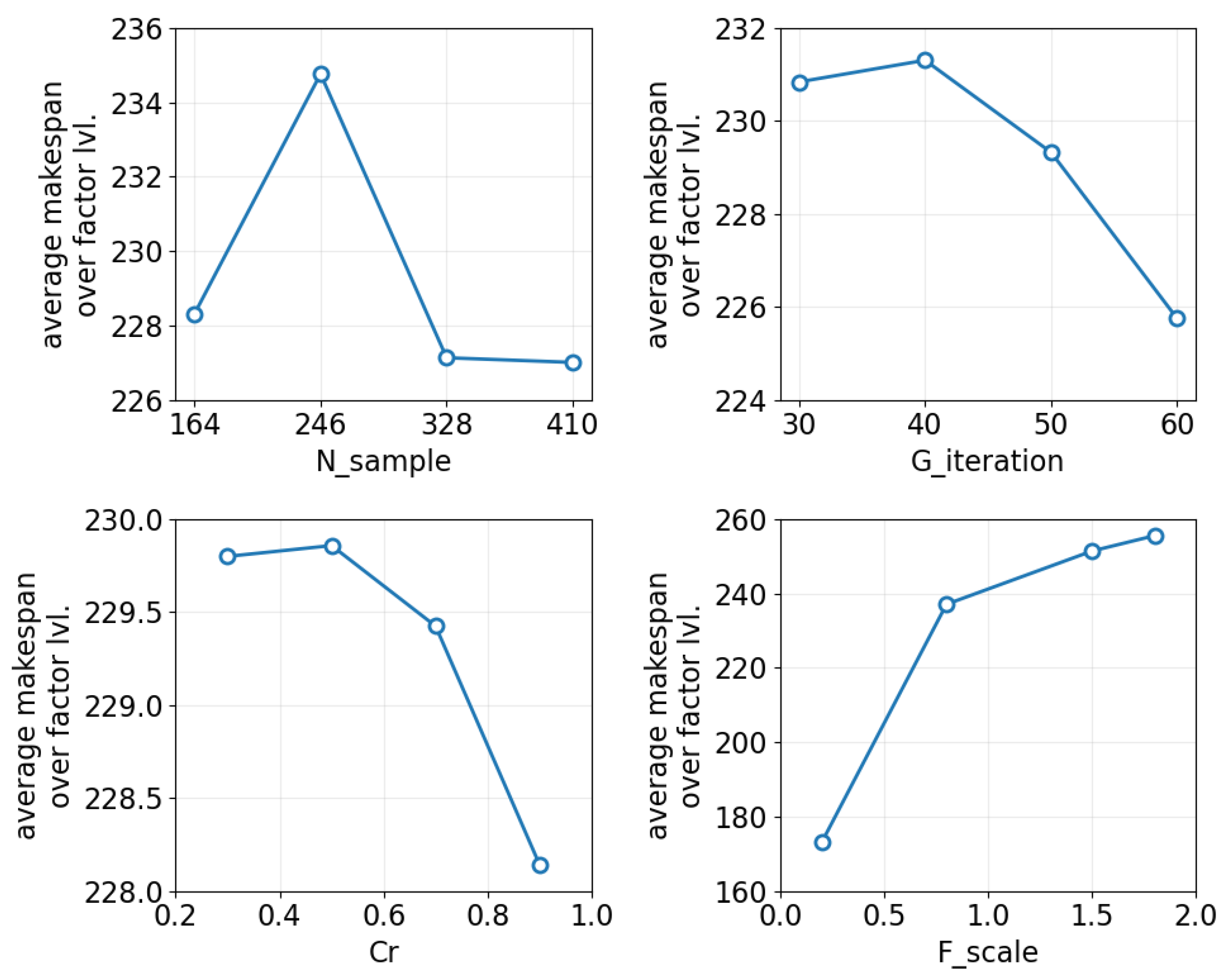
Initially, we must determine the parameters for the proposed algorithm utilizing the Taguchi experimental design process [47]. For this purpose, we select the case of $I_{82\_5\_5}$ that has $n_{\mathrm{op}}=82$ operations, a maximum of 5 available machines and 5 available factories. The algorithm is governed by five key control parameters, namely $N_{\mathrm{pop}}$ for population size, $F_{\mathrm{scale}}$ for mutation scale factor, $G_{\max }$ for the maximum number of generations, and $C_r$ for crossover probability. Each control factor was examined across four distinct levels, and the corresponding parameter configurations are recorded in

Table 3. Our range of primary parameters $N_{\mathrm{sample}}$, $G_{\max }$, $C_r$, and $F_{\mathrm{scale}}$ in the Taguchi method. Here we use $I_{82\_5\_5}$ with $n_{\mathrm{op}}=82$ operations, maximum of 5 available machines and 5 available factories.

Parameters	Factor Level
	1	2	3	4
$N_{\mathrm{sample}}$	$2n_{\mathrm{op}}$	$3n_{\mathrm{op}}$	$4n_{\mathrm{op}}$	$5n_{\mathrm{op}}$
$G_{\max }$	30	40	50	60
$C_r$	0.3	0.5	0.7	0.9
$F_{\mathrm{scale}}$	0.2	0.8	1.5	1.8

. For each control parameter configuration, the proposed algorithm was executed independently across 30 runs to ensure statistical robustness, with the mean makespan serving as the primary performance indicator. The corresponding Taguchi experimental design and the resulting observations are systematically presented in Table 3 and

Table 4. Taguchi orthogonal array and experimental results.

Exp.	Factor Levels				Average
	${\mathit{N}}_{\mathrm{sample}}$	${\mathit{G}}_{max}$	${\mathit{C}}_{\mathit{r}}$	${\mathit{F}}_{\mathrm{scale}}$	Makespan
1	1	1	1	1	169.0
2	1	2	2	2	241.1
3	1	3	3	3	251.5
4	1	4	4	4	251.1
5	2	1	2	3	260.2
6	2	2	1	4	264.4
7	2	3	4	1	180.2
8	2	4	3	2	234.2
9	3	1	3	4	257.9
10	3	2	4	3	245.2
11	3	3	1	2	236.7
12	3	4	2	1	168.8
13	4	1	4	2	236.1
14	4	2	3	1	174.1
15	4	3	2	4	248.9
16	4	4	1	3	248.9
$K_1$	913.7	923.4	919.2	692.3	–
$K_2$	939.0	925.2	919.4	948.5	–
$K_3$	908.5	917.3	917.7	1005.8	–
$K_4$	908.0	903.0	912.6	1022.3	–
$k_1$	228.4	230.9	229.8	173.1	–
$k_2$	234.8	231.3	229.9	237.1	–
$k_3$	227.1	229.3	229.4	251.5	–
$k_4$	227.0	225.8	228.2	255.6	–
Range	7.8	5.6	1.7	82.5	–
Rank	4	2	3	1	–

Note: K_i = sum of makespan values at level i; k_i = K_i/4 = average response; range = max(k_i) − min(k_i); lower rank indicates greater factor influence.

. Moreover, the impact of specific parameters on algorithm performance is visually represented in Figure 8, where the average makespan is calculated at the end of generation.

From Table 4 and Figure 8, we can order our rank of primary parameters based on their ranges of influencing average makespan, and explain their behavior. The most primary parameter influencing the algorithm is the mutation scale factor $F_{\mathrm{scale}}$. This parameter has a large range of influence on average makespan. The second important parameter is $G_{\max }$, the maximum number of generations in local iterations. If the size is excessively large, the execution time of the algorithm will increase significantly. The subsequent parameter pertains to the crossover probability $C_{\mathrm{r}}$. Increasing this parameter will trigger more crossover mechanisms, as we observe from Figure 8. A trend exists towards achieving a minimal average makespan, with the population size $N_{\mathrm{sample}}$ exerting the least influence on the algorithm’s performance. If $N_{\mathrm{sample}}$ is inadequately small, it does not sufficiently characterize the distribution of the solutions. If $N_{\mathrm{sample}}$ is excessively large, the execution time of the algorithm will increase significantly. We can see in Figure 8 that there is no benefit to using a larger number of individuals since it does not improve the average makespan. The parameters of DE presented in this study are established as follows: $N_{\mathrm{sample}}=4n_{\mathrm{op}}$, $G_{\max }=60$, $C_r=0.9$, $F_{\mathrm{scale}}=0.2$.

6. Results

6.1. Initial Testing for a Single Instance

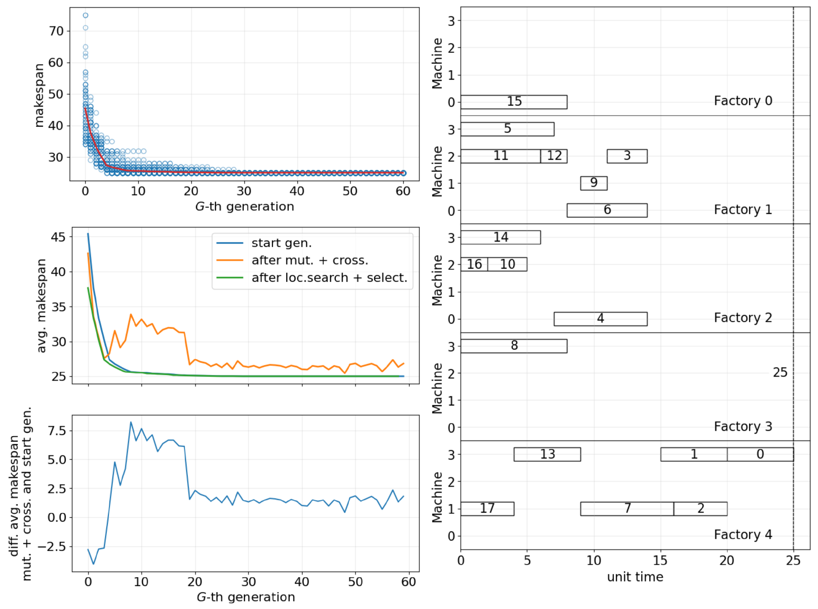
For the preliminary result, we tried $n_{\mathrm{op}}=18$ and 82 (we only show results in this article for 18 operations; see Figure 9). We have achieved convergence for all individuals to a stable makespan after 40 generations. In Figure 9, we also keep track of the average makespan over the number of individuals ($N_{\mathrm{sample}}$) for three categories: (a) in the starting stage before each generation, (b) after mutation and crossover operators, and (c) after local search and selection operator. We found that these mutation and crossover operators are aggressive to explore more search space, as we can see in the beginning of each generation that they increase dramatically and tend to be stable after generation 20. Local search and selection do not improve the average makespan significantly after generation 10.

6.2. Comparison of DE-FIAPDS with Existing Algorithm

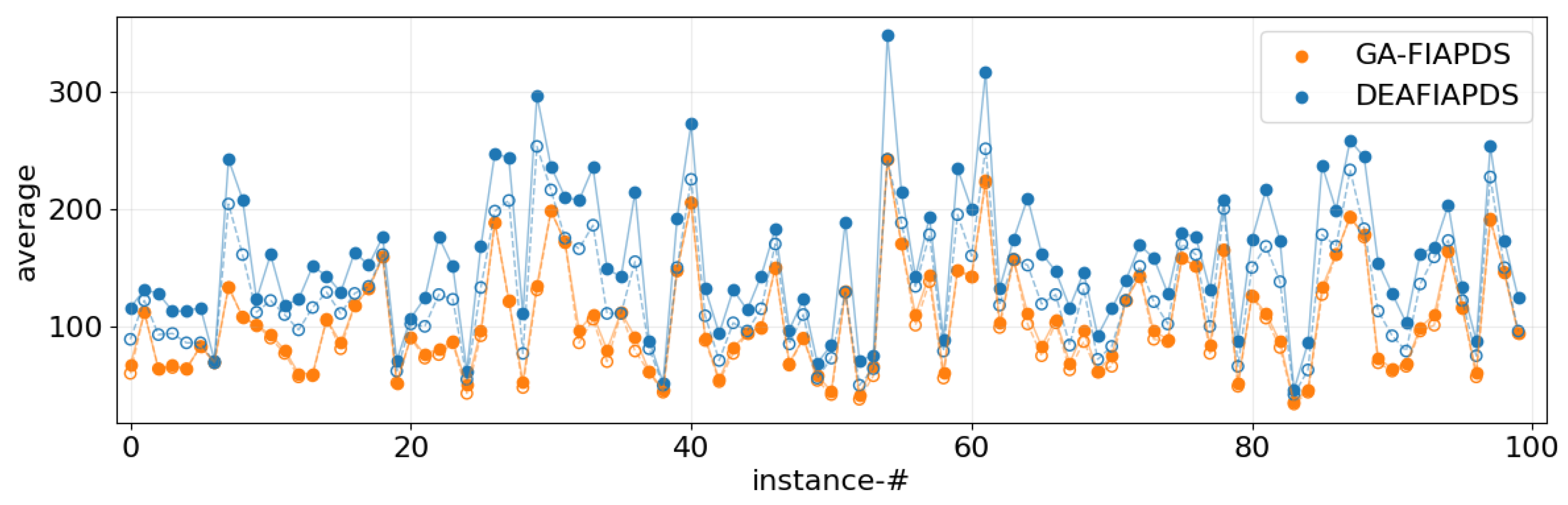
In 30 independent runs of the aforementioned algorithms on 100 randomly generated cases, our algorithm DE achieved both the average and minimum makespan, as illustrated in Figure 10. That figure shows the average makespan at the last generation and over 30 runs; the mean of this quantity over all 100 instances (including its standard deviation) for GA-FIAPDS is 106.10 (44.39) and for DE-FIAPDS it is 156.60 (59.23). The minimum average makespan for GA-FIAPDS is 36, and for DE-FIAPDS it is 46. This minimum average makespan occurred in instance 83 with $n_{\mathrm{op}}=52$, $n_{\mathrm{mac}}=6$, and $n_{\mathrm{fac}}=3$.

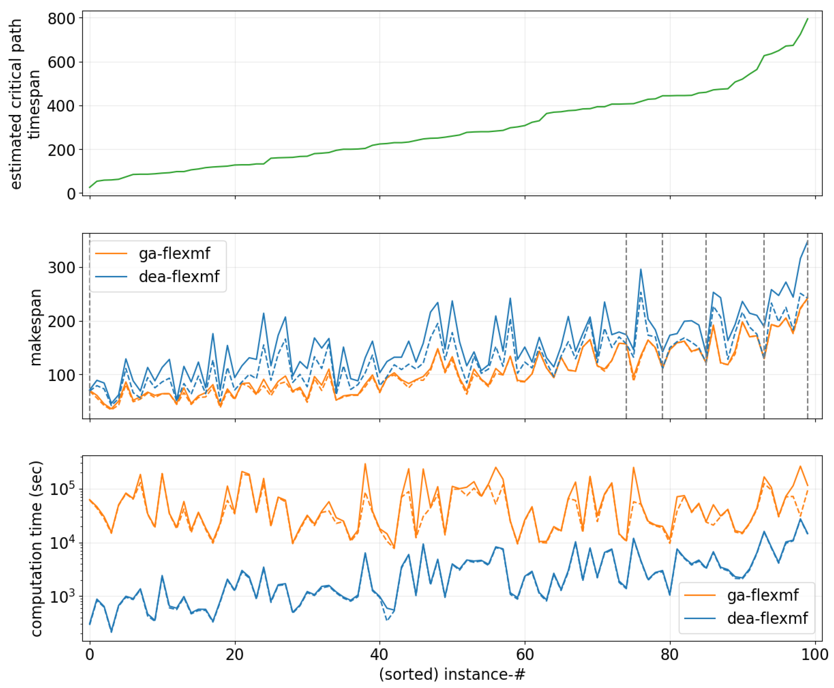
We are sorting 100 instances of data according to their critical path timespan. The critical path timespan is the total maximum processing time ${\sum }_i{p}_{im}$ along the longest path in process priority starting from the deepest children operation to root operation (see Figure 3). We only select the first found on the longest path even though there might be multiple longest paths. Doing that kind of sorting, we can see clearly the trend of implementation for DE-FIAPDS and GA-FIAPDS. Figure 11 shows a comparison between our DE-FIAPDS and GA-FIAPDS for their average makespan and computational time. DE-FIAPDS is faster in calculating the solutions.

In Figure 11, we can order approximately for every 100 instances according to their critical path timespan. We found that as the problem becomes bigger, DE-FIAPDS tends to increase its computational time. In GA-FIAPDS, we barely see any trend for this computational time, but the difference in computational time between these two algorithms is in order of approximately 100.

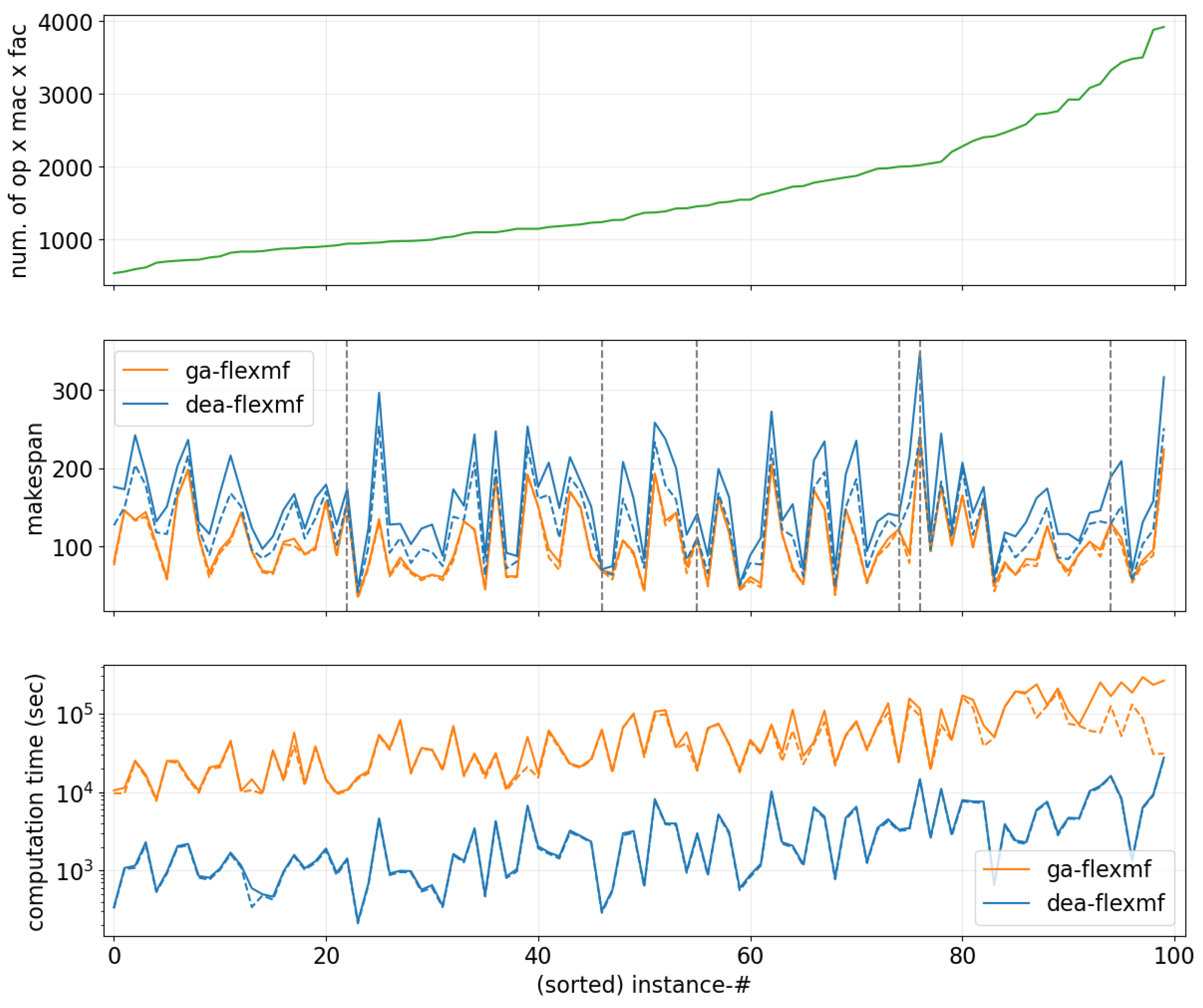
In Figure 12, we sort our results of 100 instances based on their search spaces ($n_{\mathrm{op}}\times n_{\mathrm{mac}}\times n_{\mathrm{fac}}$). The results using this sorting of problems are very clear: upward trends in computational time between GA-FIAPDS and DE-FIAPDS.

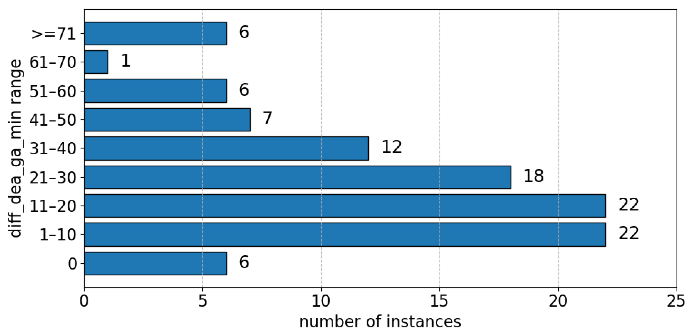
In Figure 13, we see the difference in minimum makespan between GA-FIAPDS and DE-FIAPDS. From that graph, we can see the distribution is right-skewed, with a few upper-range examples. Large disparities between the two approaches are rare, since the ranges over 50 have low representation (6, 1, and 6 cases for 51–60, 61–70, and m ≥ 71, respectively). We can suggest that GA-FIAPDS and DE-FIAPDS approaches often yield similar minimum values. Following these findings, the subsequent stage in enhancing DE is to optimize the local search and augment the complexity to get more robust outcomes.

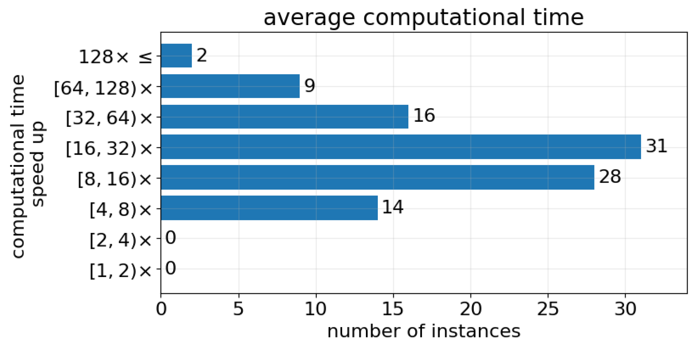
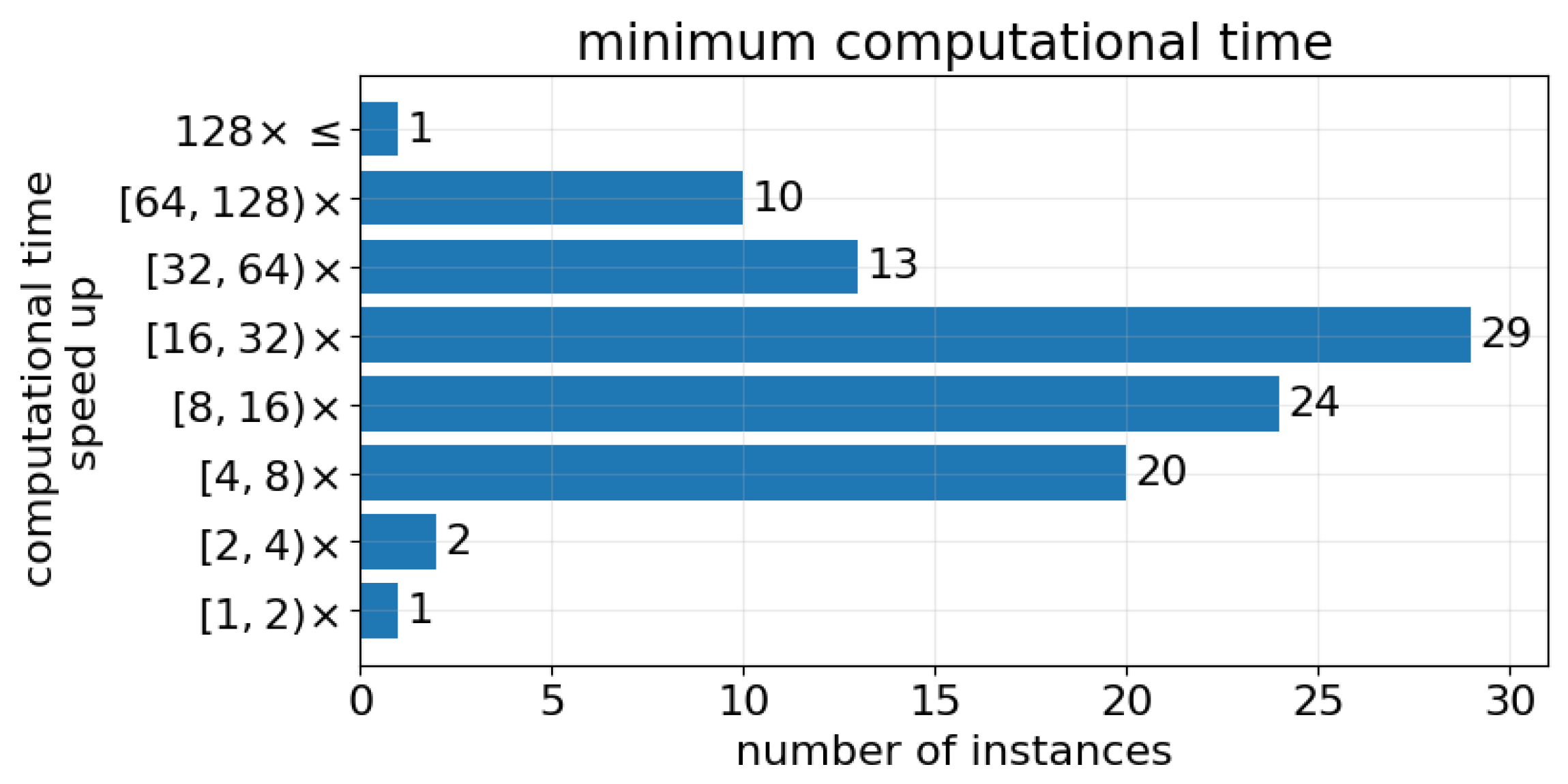
Both results in Figure 14 and Figure 15, which are the average and minimum computational time of the proposed DE-FIAPDS, are assessed against the GA-FIAPDS across 100 instances. As shown in the figure, every instance recorded a speed-up factor of at least 4×, with the majority falling within the [16, 32)× range (31 instances), followed by [8, 16)× (28 instances) and [32, 64)× (16 instances). Remarkably, no instance was observed where the GA-FIAPDS matched or surpassed the computational speed of DE-FIAPDS, confirming the algorithm’s consistent superiority. These results suggest that DE-FIAPDS offers a substantial reduction in computational time compared to GA-FIAPDS, making it a highly practical choice for solving large-scale optimization problems efficiently.

7. Conclusions and Future Research

From the scheduling problem FIAPDS that we have defined, we have implemented two heuristic evolutionary algorithms: DE-FIAPDS and GA-FIAPDS. We compute the average and minimum makespan for all 100 different instances. We found that for all 30 different independent executions, the algorithm converges to the same minimum makespan.

In Figure 13, the DE-FIAPDS and GA-FIAPDS approaches often yield similar minimum values; considerable variation exists across the dataset, with most divergences remaining within moderate bounds. In the future, the local search should be optimized and complexity added to DE-FIAPDS to make this algorithm faster and help it find the best minimum makespan. Overall, the performance of both algorithms was similar, but the computational time of DE-FIAPDS is much faster (around 100 times faster than GA-FIAPDS). If we take a look at the minimum makespan over 30 runs, these algorithms actually produce approximately the same result.

This study evaluates two algorithms for scenarios involving flexible machines with a constraint of several available machines and flexible factories where local search demands additional time, reducing its efficiency. We implement all the algorithms using standard Python libraries: NumPy and Numba. There is another implementation of this type of algorithm in Python: Pymoo. This module is not very easy to adopt for solving our problem, and that Python library does not support Numba. In future research, it is necessary to improve the implementation to utilize a GPU or even a parallel programming technique.

References

1. Pinedo, M.L. Scheduling: Theory, Algorithms, and Systems; Springer International Publishing: Cham, Switzerland, 2022. [Google Scholar] [CrossRef]
2. Taillard, E. Benchmarks for basic scheduling problems. Eur. J. Oper. Res. 1993, 64, 278–285. [Google Scholar] [CrossRef]
3. Destouet, C.; Tlahig, H.; Bettayeb, B.; Mazari, B. Flexible job shop scheduling problem under Industry 5.0: A survey on human reintegration, environmental consideration and resilience improvement. J. Manuf. Syst. 2023, 67, 155–173. [Google Scholar] [CrossRef]
4. Mraihi, T.; Driss, O.B.; EL-Haouzi, H.B. Distributed Permutation Flow Shop Scheduling Problem with Worker flexibility: Review, trends and model proposition. Expert Syst. Appl. 2024, 238, 121947. [Google Scholar] [CrossRef]
5. Wang, B.; Zhou, H.; Li, X.; Yang, G.; Zheng, P.; Song, C.; Yuan, Y.; Wuest, T.; Yang, H.; Wang, L. Human Digital Twin in the context of Industry 5.0. Robot. Comput.-Integr. Manuf. 2024, 85, 102626. [Google Scholar] [CrossRef]
6. Putri Ardyanti, A.A.A.; Xie, Z.; Karnyoto, A.S.; Pardamean, B.; Estiyanti, N.M. Mapping the Scientific Landscape of Integrated Scheduling Towards Industry 5.0 with A Bibliometric Analysis. In Procedia Computer Science; Vagan, S., Feng, L., Dong, R., Eds.; Elsevier B.V.: Amsterdam, The Netherlands, 2025; Volume 253, pp. 84–93. [Google Scholar] [CrossRef]
7. Yang, Y.; Zhu, X.; Haghani, A. Multiple Equipment Integrated Scheduling and Storage Space Allocation in Rail–Water Intermodal Container Terminals Considering Energy Efficiency. Transp. Res. Rec. 2019, 2673, 199–209. [Google Scholar] [CrossRef]
8. Chansombat, S.; Pongcharoen, P.; Hicks, C. A mixed-integer linear programming model for integrated production and preventive maintenance scheduling in the capital goods industry. Int. J. Prod. Res. 2019, 57, 61–82. [Google Scholar] [CrossRef]
9. Mallikarjuna, K.; Veeranna, V.; Reddy, K.H. A new meta-heuristics for optimum design of loop layout in flexible manufacturing system with integrated scheduling. Int. J. Adv. Manuf. Technol. 2016, 84, 1841–1860. [Google Scholar] [CrossRef]
10. Yang, D.; Xie, Z.; Zhang, C. Multi-flexible integrated scheduling algorithm for multi-flexible integrated scheduling problem with setup times. Math. Biosci. Eng. 2023, 20, 9781–9817. [Google Scholar] [CrossRef] [PubMed]
11. Lu, J.; Xu, L.; Jin, J.; Shao, Y. A Mixed Algorithm for Integrated Scheduling Optimization in AS/RS and Hybrid Flowshop. Energies 2022, 15, 7558. [Google Scholar] [CrossRef]
12. Li, X.; Lu, J.; Yang, C.; Wang, J. Research of Flexible Assembly Job-Shop Batch-Scheduling Problem Based on Improved Artificial Bee Colony. Front. Bioeng. Biotechnol. 2022, 10, 909548. [Google Scholar] [CrossRef] [PubMed]
13. Zhang, X.; Xie, Z.; Shao, X.; Xia, Y. An integrated scheduling method for personalized products with no-wait constraints. Int. J. Adv. Manuf. Technol. 2022, 122, 279–290. [Google Scholar] [CrossRef]
14. Gao, Y.; Xie, Z.; Yu, X. A hybrid algorithm for integrated scheduling problem of complex products with tree structure. Multimed. Tools Appl. 2020, 79, 32285–32304. [Google Scholar] [CrossRef]
15. Cheng, B.Y.; Leung, J.Y.T.; Li, K. Integrated scheduling of production and distribution to minimize total cost using an improved ant colony optimization method. Comput. Ind. Eng. 2015, 83, 217–225. [Google Scholar] [CrossRef]
16. Zhang, S.; Wang, S. Flexible assembly job-shop scheduling with sequence-dependent setup times and part sharing in a dynamic environment: Constraint programming model, mixed-integer programming model, and dispatching rules. IEEE Trans. Eng. Manag. 2018, 65, 487–504. [Google Scholar] [CrossRef]
17. Wang, D.Y.; Grunder, O.; El Moudni, A. Integrated scheduling of production and distribution operations: A review. Int. J. Ind. Syst. Eng. 2015, 19, 94–122. [Google Scholar] [CrossRef]
18. Cheng, B.Y.; Leung, J.Y.T.; Li, K. Integrated scheduling on a batch machine to minimize production, inventory and distribution costs. Eur. J. Oper. Res. 2017, 258, 104–112. [Google Scholar] [CrossRef]
19. Jia, Z.H.; Huo, S.Y.; Li, K.; Chen, H.P. Integrated scheduling on parallel batch processing machines with non-identical capacities. Eng. Optim. 2020, 52, 715–730. [Google Scholar] [CrossRef]
20. He, Z.; Guo, Z.; Wang, J. Integrated scheduling of production and distribution operations in a global MTO supply chain. Enterp. Inf. Syst. 2019, 13, 490–514. [Google Scholar] [CrossRef]
21. Low, C.; Li, R.K.; Chang, C.M. Integrated scheduling of production and delivery with time windows. Int. J. Prod. Res. 2013, 51, 897–909. [Google Scholar] [CrossRef]
22. Wan, X.Q.; Yan, H.S. Integrated scheduling and self-reconfiguration for assembly job shop in knowledgeable manufacturing. Int. J. Prod. Res. 2015, 53, 1746–1760. [Google Scholar] [CrossRef]
23. Yabo, L.; Yang, W.; Feng, Z. Optimization Algorithm for Balancing and Sequencing Mixed Assembly Line; Lecture Notes in Computer Science; Springer: Berlin/Heidelberg, Germany, 2014; pp. 422–431. [Google Scholar] [CrossRef]
24. Du, H.; Liu, D.; Zhang, M.H. A hybrid algorithm based on particle swarm optimization and artificial immune for an assembly job shop scheduling problem. Math. Probl. Eng. 2016, 2016, 3938679. [Google Scholar] [CrossRef]
25. Lei, Q.; Guo, W.; Song, Y. Integrated scheduling algorithm based on an operation relationship matrix table for tree-structured products. Int. J. Prod. Res. 2018, 56, 5437–5456. [Google Scholar] [CrossRef]
26. Zheng, Y.; Xu, M.; Wang, Z.; Xiao, Y. A Genetic Algorithm for Integrated Scheduling of Container Handling Systems at Container Terminals from a Low-Carbon Operations Perspective. Sustainability 2023, 15, 6035. [Google Scholar] [CrossRef]
27. Zeng, M.; Sadeghzadeh, K.; Xiong, T. A three-echelon based sustainable supply chain scheduling decision-making framework under the blockchain environment. Int. J. Prod. Res. 2023, 61, 4951–4971. [Google Scholar] [CrossRef]
28. Qiu, F.; Geng, N.; Wang, H. An improved memetic algorithm for integrated production scheduling and vehicle routing decisions. Comput. Oper. Res. 2023, 152, 106127. [Google Scholar] [CrossRef]
29. Berghman, L.; Kergosien, Y.; Billaut, J.C. A review on integrated scheduling and outbound vehicle routing problems. Eur. J. Oper. Res. 2023, 311, 1–23. [Google Scholar] [CrossRef]
30. Huang, S.; Zhou, C.; Xiong, N.; Yang, S.H.; Qin, Y.; Zhang, Q. A general real-time control approach of intrusion response for industrial automation systems. IEEE Trans. Syst. Man Cybern. Syst. 2016, 46, 1021–1035. [Google Scholar] [CrossRef]
31. Tan, W.; Yuan, X.; Wang, J.; Xu, H.; Wu, L. Multi-objective teaching–learning-based optimization algorithm for carbon-efficient integrated scheduling of distributed production and distribution considering shared transportation resource. J. Clean. Prod. 2023, 406, 137061. [Google Scholar] [CrossRef]
32. Wang, J.; Yao, S.; Sheng, J.; Yang, H. Minimizing total carbon emissions in an integrated machine scheduling and vehicle routing problem. J. Clean. Prod. 2019, 229, 1004–1017. [Google Scholar] [CrossRef]
33. Zhai, S.; Riess, A.; Reinhart, G. Formulation and solution for the predictive maintenance integrated job shop scheduling problem. In Proceedings of the IEEE International Conference on Prognostics and Health Management (ICPHM), San Francisco, CA, USA, 17–20 June 2019. [Google Scholar] [CrossRef]
34. Ladj, A.; Tayeb, F.B.S.; Varnier, C. Tailored Genetic Algorithm for Scheduling Jobs and Predictive Maintenance in a Permutation Flowshop. In Proceedings of the IEEE International Conference on Emerging Technologies and Factory Automation (ETFA), Torino, Italy, 4–7 September 2018; pp. 524–531. [Google Scholar] [CrossRef]
35. Yadav, N.; Tanksale, A. An integrated routing and scheduling problem for home healthcare delivery with limited person-to-person contact. Eur. J. Oper. Res. 2022, 303, 1100–1125. [Google Scholar] [CrossRef]
36. Di Martinelly, C.; Duenas, A.; Pham, D. Integration of operating room advance scheduling and allocation scheduling while considering the resource constraints: A multiobjective genetic algorithm approach. In Proceedings of the ILS—Information Systems, Logistics and Supply Chain, Proceedings, INSA Lyon, Villeurbanne, France, 8–11 July 2018; pp. 714–724. [Google Scholar]
37. Xie, Z.; Yang, D.; Ma, M.; Yu, X. An improved artificial bee colony algorithm for the flexible integrated scheduling problem using networked devices collaboration. Int. J. Coop. Inf. Syst. 2020, 29, 2040003. [Google Scholar] [CrossRef]
38. Gao, Y.; Xie, Z.; Yang, D.; Yu, X. Flexible integrated scheduling algorithm based on remaining work probability selection coding. Expert Syst. 2021, 38, e12683. [Google Scholar] [CrossRef]
39. Gao, Y.; Xie, Z.; Jia, Q.; Yu, X. An Effective Memetic Algorithm for the Distributed Integrated Scheduling of Tree-Structured Products. Int. J. Coop. Inf. Syst. 2021, 30, 2150001. [Google Scholar] [CrossRef]
40. Yuan, Y.; Xu, H. Flexible job shop scheduling using hybrid differential evolution algorithms. Comput. Ind. Eng. 2013, 65, 246–260. [Google Scholar] [CrossRef]
41. Kailasa, S.; Wang, T.; Barba, L.A.; Betcke, T. PyExaFMM: An exercise in designing high-performance software with Python and Numba. Comput. Sci. Eng. 2023, 24, 77–84. [Google Scholar] [CrossRef]
42. Ye, F.; Zhao, J.; Shirako, J.; Sarkar, V. Concrete Type Inference for Code Optimization using Machine Learning with SMT Solving. Proc. Program. Lang. 2023, 7, 773–800. [Google Scholar] [CrossRef]
43. Bartlett, J.; Uchytil, C.; Storti, D. High-Productivity Parallelism With Python Plus Packages (But Without a Cluster). Comput. Sci. Eng. 2021, 23, 38–46. [Google Scholar] [CrossRef]
44. Storn, R.; Price, K. Differential Evolution—A Simple and Efficient Heuristic for global Optimization over Continuous Spaces. J. Glob. Optim. 1997, 11, 341–359. [Google Scholar] [CrossRef]
45. Opara, K.R.; Arabas, J. Differential Evolution: A survey of theoretical analyses. Swarm Evol. Comput. 2019, 44, 546–558. [Google Scholar] [CrossRef]
46. Lam, S.K.; Pitrou, A.; Seibert, S. Numba: A LLVM-based Python JIT compiler. In Proceedings of the Second Workshop on the LLVM Compiler Infrastructure in HPC, New York, NY, USA, 15 November 2015; LLVM ’15. [Google Scholar] [CrossRef]
47. Montgomery, D.C. Design and Analysis of Experiments, 10th ed.; Wiley: Hoboken, NJ, USA, 2020. [Google Scholar]
Figure 1. A sample for complex product.
Axioms 15 00566 g001
Figure 2. The diagram of assembly operations, factory assignment (including machine assignment in each factory). All the distances are measured in unit time.
Axioms 15 00566 g002
Figure 3. Hierarchical assembly operation in the form of a tree-like structure.
Axioms 15 00566 g003
Figure 4. A tri-chain of one possible solution to FIAPDS. To get the first row (operation chain), every immediate predecessor of an operation O i must be put before (on the left side) the position of that operation. With this rule, we always end up having the root operation O 0 at the last position (right) of a tri-chain. For the second row (machine chain), we can assign any available machine for each operation. For the third row (factory chain), we can assign any factory for each operation.
Axioms 15 00566 g004
Figure 5. Representing the problem in real-valued vector X i , g and connecting into three-vector code ( O i , g , M i , g , and F i , g ). In the bottom part, we mentioned a tri-chain variable that represents the assignment of each operation to machine and factory. In that image, we have 18 operations, four machines, and five factories. The transformation between real-valued vectors X i , g and three-vector code will be explained in a later section.
Axioms 15 00566 g005
Figure 6. Main stage DE-FIAPDS.
Axioms 15 00566 g006
Figure 7. Gantt chart of five factories after decoding of three-vector code. The vertical dashed lines are visual aids to show D f i , f j (the distance between factories, in unit time). The blue rectangles in some operations show the sequence of critical operations. The red dashed line means the makespan.
Axioms 15 00566 g007
Figure 8. All average makespan in the Taguchi method for all four parameters N sample , G max , C r , and F scale . We set this parameter with the factor level of 3-4-4-1 for 100 instances.
Axioms 15 00566 g008
Figure 9. An evolution of makespan for a single run of 18 operations with up to four available machines and five machines. (Top left): the evolution of makespan for all individuals is drawn by the blue circle. The red line is the average makespan over these individuals. (Middle left): Comparison of average makespan for all three categories (at starting generation, after mutation and crossover, and after local search and selection). (Bottom left): The difference in average makespan between (mutation + crossover) and at starting generation. (Right): A Gantt chart for the best solution of FIAPDS with 18 operations.
Axioms 15 00566 g009
Figure 10. Average and minimum makespan comparison between DE-FIAPDS and GA-FIAPDS. Dashed line with circle is for minimum makespan, and solid line with disk is for average makespan.
Axioms 15 00566 g010
Figure 11. The makespan and computational time of DE compared with GA when we sort the 100 instances based on critical path timespan. In the middle plot, we add a dashed vertical line to indicate the instances that have the same minimum makespan over the population.
Axioms 15 00566 g011
Figure 12. The makespan and computational time of DE compared with GA when we sort the 100 instances based on the search space ( n op × n mac × n fac ). In the middle plot, we add a dashed vertical line to indicate the instances that have the same minimum makespan over the population.
Axioms 15 00566 g012
Figure 13. The difference in minimum makespan between DE and GA. We clearly observe that DE can achieve the same results on its minimum makespan over population compared to GA.
Axioms 15 00566 g013
Figure 14. The average computational time of DE compared with GA when we sort the 100 instances based on computational time speedup.
Axioms 15 00566 g014
Figure 15. The minimum computational time of DE compared with GA when we sort the 100 instances based on computational time speedup.
Axioms 15 00566 g015