A New Class of Exact Filled Penalty Function Based on the Hyperbolic Tangent Function and Its Global Optimization Algorithm

Abstract

A new class of smooth exact penalty functions, constructed using the hyperbolic tangent (tanh) function, is proposed for solving constrained global optimization problems. The tanh function is chosen because of its unique mathematical properties: it is monotonic, bounded, infinitely differentiable, and provides a uniform approximation of the absolute value function with an explicit error bound of $O(1/(\gamma e\left)\right)$. These properties make it particularly suitable for constructing smooth penalty functions that preserve exactness. The proposed penalty function exhibits both smoothness and exactness: it is continuously differentiable, and for a sufficiently large penalty parameter, its local minimizers coincide exactly with those of the original constrained problem. In addition, by integrating a filling term, a novel filled penalty function is constructed that enables the algorithm to escape from a current local minimizer and locate a better one. Leveraging this filled penalty function, a global optimization algorithm is designed that performs local minimization and filling stages alternately. The convergence properties of the algorithm are rigorously established; it is shown that the sequence of objective function values is strictly decreasing and that the termination point constitutes a global approximate optimal solution. Finally, numerical experiments on 18 benchmark problems, along with statistical significance tests and performance profiles, confirm the effectiveness and competitiveness of the proposed approach against traditional quadratic penalty methods and modern solvers such as IPOPT and ALM.

1. Introduction

Constrained optimization problems arise frequently in engineering, economics, management science, and many other fields. A general constrained optimization problem can be formulated as

$$\begin{array}{cc}\hfill min& f\left(x\right)\hfill \\ \hfill \mathrm{s}.\mathrm{t}.& g_i\left(x\right)\le 0,i=1,2,\dots ,m,\hfill \end{array}$$

where $x\in {\mathbb{R}}^n$, $f:{\mathbb{R}}^n\to \mathbb{R}$ and $g_i:{\mathbb{R}}^n\to \mathbb{R}$ are continuously differentiable functions. The feasible set is denoted by $X=\{x\in {\mathbb{R}}^n:g_i\left(x\right)\le 0,i=1,\dots ,m\}$.

Penalty function methods are among the most important approaches for solving constrained optimization problems [1,2,3]. The basic idea is to transform the constrained problem into one or a sequence of unconstrained problems by adding a penalty term that penalizes constraint violations. Traditional penalty functions, such as the quadratic penalty function, require the penalty parameter to tend to infinity, which often leads to ill-conditioning and numerical difficulties. Exact penalty functions, such as the ${\mathsf{\ell }}_1$ exact penalty function, can achieve exactness with a finite penalty parameter, but they are non-differentiable at constraint boundaries, limiting the application of gradient-based optimization algorithms.

To overcome these drawbacks, smoothing techniques have been introduced. Various smooth approximations of the ${\mathsf{\ell }}_1$ norm or max functions have been proposed to construct smooth exact penalty functions. Recent developments in this area include the unified smoothing approach for ${\mathsf{\ell }}_1$-exact penalty functions presented by a research group in 2025, which establishes sufficient conditions for the existence of local minimizers and linear convergence rates for a class of smoothing methods [4]. Additionally, a new smooth quadratic penalty function that is continuously differentiable has been proposed, with detailed error estimations between the smooth penalty problem and the original problem [5]. A general perspective on smooth exact penalty functions has also been developed, providing new simple proofs of local exactness that generalize existing results [6]. Among various smoothing functions, the hyperbolic tangent (tanh) function is chosen for several compelling reasons. First, the tanh function is infinitely differentiable ($C^{\infty }$), which enables the use of higher-order optimization methods. Second, it is monotonic and bounded, providing a stable and controlled approximation of the nonsmooth absolute value function. Third, it admits an explicit uniform approximation error bound of $\left|t\right|-\left|t\right|tanh\left(\gamma \right|t\left|\right)\le 1/\left(2\gamma e\right)$, which is sharper than many existing smoothing approaches. Fourth, its derivative has a simple closed form with an explicit bound, facilitating theoretical analysis. These properties make tanh particularly attractive for constructing smooth exact penalty functions with guaranteed convergence properties. In this paper, a new class of smooth exact penalty functions based on the tanh function is proposed. The proposed penalty function is continuously differentiable for any finite penalty parameter and maintains exactness when the penalty parameter is sufficiently large.

Another major difficulty in global optimization is how to escape from a current local minimizer to find a better one. The filled function method, originally proposed by Ge [7], is an effective approach to addressing this issue. The idea is to construct an auxiliary function (called a filled function) at a current local minimizer, whose minimizer provides a better initial point for the original problem. In recent years, significant progress has been made in filled function methods. Wang et al. (2023) proposed a new filled function for constrained global optimization with a single adjustable parameter [8]. A new class of continuously differentiable filled functions with two parameters was introduced in 2024, featuring no exponential or logarithmic terms to reduce computational overflow [9]. A novel one-parameter filled function method was developed in 2024 with applications to pathological analysis [10]. More recently, a new class of one-parameter filled functions was proposed in 2025–2026, demonstrating superior performance in global optimization problems with fewer iterations [11]. Additionally, the EDECT algorithm, which hybridizes the filled function and DIRECT methods, was introduced in 2026 as a deterministic approach for global optimization [12]. A typical form of a filled function is given by [13]

$$T_1(x,x^{*},\tau )={\displaystyle \frac{\varphi \left(\tau [f\left(x\right)-f\left(x^{*}\right)+h]\right)}{\parallel x-x^{*}\parallel }},$$

where $\tau \ge 1$ and $h>0$ are parameters, $x^{*}$ is a local minimizer of f, and $\varphi \left(t\right)$ satisfies $\varphi \left(0\right)=0$, ${\varphi }^{\prime }\left(t\right)>0$ for $t>-t_1$ ($t_1\ge 0$), and ${lim}_{t\to \infty }t{\varphi }^{\prime }\left(t\right)/\varphi \left(t\right)=0$. By minimizing such a filled function, one can obtain a point $\overline{x}$ with $f\left(\overline{x}\right)<f\left(x^{*}\right)$, thus escaping the current basin and progressing toward the global minimum.

In recent years, the combination of penalty functions and filling properties has attracted considerable attention [14,15,16,17]. Tang et al. (2022) proposed a class of lower-order smoothed objective penalty functions with filling properties [14]. Their filled penalty function takes the form

$$H_{ϵ}(x,\overline{x},M,\rho )=Q(f\left(x\right)-M)+\rho {\displaystyle \sum _{i=1}^m}{p}_{ϵ}^{1/2}\left(g_i\left(x\right)\right)+\rho p_{ϵ}^{1/2}(f\left(x\right)-f\left(\overline{x}\right)+2ϵ),$$

where $\overline{x}$ is a known local minimizer, Q and $p_{ϵ}^{1/2}$ are smooth approximations of the plus function, and $\rho >0$, $ϵ>0$ are parameters. This function successfully combines exactness with filling properties, allowing the algorithm to escape local minima. However, the construction relies on a piecewise smoothing technique that may introduce additional parameters and complexity.

To better position the proposed method within the existing literature, a detailed comparison with the author’s previous works [14,15,16,17] is provided below.

Table 1. Comparison between the proposed method and previous works by the author.

Feature	Previous Works ([14,15,16,17])	This Work
Smoothing mechanism	Piecewise polynomial/barrier	Hyperbolic tangent (tanh)
Differentiability	$C^1$ or $C^2$	$C^{\infty }$ (infinitely differentiable)
Number of smoothing parameters	Multiple	Single ($\gamma$)
Explicit approximation error	Not provided	$1/\left(2\gamma e\right)$ (uniform)
Filling term integration	Yes (except 2019)	Yes
Filling term monotonicity	Not explicitly used	Explicitly proved
Gradient Lipschitz bound	Not provided	Explicitly derived
Penalty exactness	Yes	Yes

summarizes the key differences between the proposed tanh-based formulation and these earlier approaches.

Compared with the existing filled penalty functions in [14,16,17], the proposed tanh-based formulation offers several distinct advantages. First, the tanh function provides a uniform approximation to the absolute value function with an explicit error bound of $O(1/(\gamma e\left)\right)$, which is sharper than the piecewise smoothing approach used in the author’s previous works. Second, the proposed formulation has a simpler structure—it avoids piecewise definitions and relies on a single smoothing parameter $\gamma$ rather than multiple smoothing parameters. Third, the tanh-based penalty function enjoys a bounded gradient with an explicit Lipschitz constant,which was not established in the earlier works. Fourth, the filling term $s_{\gamma }\left(t\right)=\left|t\right|tanh\left(\gamma \right|t\left|\right)$ is proven to be monotonically increasing for $t>0$ and decreasing for $t<0$ (Lemma 1), ensuring the filling properties with minimal parameter tuning. These advantages, summarized in Table 1, clearly distinguish the present contribution from the author’s prior research and represent a genuine advancement in the field of smoothed penalty methods for constrained global optimization.

To summarize, the main contributions of this work are threefold:

• A new class of smooth exact penalty functions based on the hyperbolic tangent function is proposed, with an explicit uniform approximation error bound of $O(1/(\gamma e\left)\right)$ and a bounded gradient with known Lipschitz constant.
• A filled penalty function is constructed by incorporating a filling term $s_{\gamma }\left(t\right)=\left|t\right|tanh\left(\gamma \right|t\left|\right)$, which preserves the filling properties with minimal parameter tuning.
• A global optimization algorithm (TFP-GO) is developed and analyzed, with convergence guarantees, and its effectiveness is validated on 18 benchmark problems with statistical significance tests and performance profiles.

The remainder of this paper is organized as follows. Section 2 introduces the new smooth exact penalty function based on the tanh function and proves its exactness. Section 3 presents the filled penalty function and its properties. Section 4 describes the global optimization algorithm and provides convergence analysis. Section 5 reports numerical experimental results on 18 benchmark problems, including performance profiles. Section 6 discusses the method’s limitations and future directions. Section 7 concludes the paper.

2. A New Smooth Exact Penalty Function Based on Tanh

2.1. Definition and Properties

First, the ${\mathsf{\ell }}_1$ exact penalty function for problem (P) is recalled:

$$P_1(x,\sigma )=f\left(x\right)+\sigma {\varphi }_1\left(x\right),$$

where $\sigma >0$ is the penalty parameter and

$${\varphi }_1\left(x\right)={\displaystyle \sum _{i=1}^m}max\{0,g_i\left(x\right)\}.$$

The ${\mathsf{\ell }}_1$ penalty function is exact but non-differentiable.

To smooth the nonsmooth term $max\{0,t\}$, the hyperbolic tangent function is introduced. Define the smoothing function $s_{\gamma }\left(t\right)$ as

$$s_{\gamma }\left(t\right)=\left|t\right|tanh\left(\gamma \right|t\left|\right),\gamma >0.$$

It is easy to verify that $s_{\gamma }\left(t\right)$ is continuously differentiable and satisfies ${lim}_{\gamma \to \infty }{s}_{\gamma }\left(t\right)=\left|t\right|$.

Based on $s_{\gamma }\left(t\right)$, a smooth approximation of ${\varphi }_1\left(x\right)$ is constructed:

$${\varphi }_s(x,\gamma )={\displaystyle \frac{1}{2}}{\displaystyle \sum _{i=1}^m}\left[g_i\left(x\right)+s_{\gamma }\left(g_i\left(x\right)\right)\right].$$

Note that $max\{0,t\}=(t+|t\left|\right)/2$, so ${\varphi }_s(x,\gamma )$ approximates ${\varphi }_1\left(x\right)$ as $\gamma \to \infty$.

Finally, the new smooth exact penalty function is defined as

$$P_s(x,\sigma ,\gamma )=f\left(x\right)+\sigma {\varphi }_s(x,\gamma ).$$

2.2. Exactness Analysis

The following theorem establishes the exactness of the proposed penalty function. A detailed proof with explicit error bounds is provided.

Theorem 1.

Let $x^{*}$ be a local optimal solution of the original problem satisfying the linear independence constraint qualification (LICQ) and the second-order sufficient condition at $x^{*}$. Then there exists $\overline{\sigma }>0$ such that for all $\sigma \ge \overline{\sigma }$ and sufficiently large γ, $x^{*}$ is also a local minimizer of $P_s(x,\sigma ,\gamma )$.

Proof. 

Consider the difference between $P_s(x,\sigma ,\gamma )$ and the ${\mathsf{\ell }}_1$ exact penalty function $P_1(x,\sigma )$:

$$\begin{array}{cc}\hfill |P_s(x,\sigma ,\gamma )-P_1(x,\sigma )|& =\sigma |{\varphi }_s(x,\gamma )-{\varphi }_1\left(x\right)|\hfill \\ \hfill & \le \sigma {\displaystyle \sum _{i=1}^m}|s_{\gamma }\left(g_i\left(x\right)\right)-|g_i\left(x\right)\left|\right|.\hfill \end{array}$$

(1)

For any $t\in \mathbb{R}$, using $s_{\gamma }\left(t\right)=\left|t\right|tanh\left(\gamma \right|t\left|\right)$ and the inequality $1-tanh\left(u\right)\le {\mathrm{e}}^{-2u}$ for $u\ge 0$, the following holds:

$$|s_{\gamma }\left(t\right)-\left|t\right||=\left|t\right|(1-tanh\left(\gamma \right|t\left|\right))\le \left|t\right|{\mathrm{e}}^{-2\gamma \left|t\right|}.$$

The function $u{\mathrm{e}}^{-2\gamma u}$ attains its maximum at $u=1/\left(2\gamma \right)$ with value $1/\left(2\gamma \mathrm{e}\right)$. Hence,

$$|s_{\gamma }\left(t\right)-\left|t\right||\le {\displaystyle \frac{1}{2\gamma \mathrm{e}}}\mathrm{for}\mathrm{all}t\in \mathbb{R}.$$

Therefore, from (1)

$$|P_s(x,\sigma ,\gamma )-P_1(x,\sigma )|\le \sigma ·{\displaystyle \frac{m}{2\gamma \mathrm{e}}}.$$

Thus, $P_s(x,\sigma ,\gamma )$ converges uniformly to $P_1(x,\sigma )$ as $\gamma \to \infty$ on any bounded set.

By the exactness of the ${\mathsf{\ell }}_1$ penalty function (see, e.g., [1]), there exists $\overline{\sigma }>0$ such that for all $\sigma \ge \overline{\sigma }$, $x^{*}$ is a strict local minimizer of $P_1(x,\sigma )$. That is, there exists $\delta >0$ such that

$$P_1(x,\sigma )>P_1(x^{*},\sigma )\forall x\in B(x^{*},\delta )\setminus \left\{x^{*}\right\},$$

where $B(x^{*},\delta )$ denotes the open ball of radius $\delta$ centered at $x^{*}$.

Now, for any x with $\parallel x-x^{*}\parallel =\delta /2$, it follows from the uniform convergence that for sufficiently large $\gamma$,

$$|P_s(x,\sigma ,\gamma )-P_1(x,\sigma )|\le {\displaystyle \frac{\sigma m}{4\gamma e}}\le {\displaystyle \frac{1}{4}}\underset{y\in \partial B(x^{*},\delta /2)}{min}[P_1(y,\sigma )-P_1(x^{*},\sigma )].$$

Consequently,

$$P_s(x,\sigma ,\gamma )\ge P_1(x,\sigma )-{\displaystyle \frac{1}{4}}\mathrm{\Delta }>P_1(x^{*},\sigma )+{\displaystyle \frac{3}{4}}\mathrm{\Delta }>P_s(x^{*},\sigma ,\gamma ),$$

where $\mathrm{\Delta }={min}_{y\in \partial B(x^{*},\delta /2)}[P_1(y,\sigma )-P_1(x^{*},\sigma )]>0$. Hence, $x^{*}$ is a strict local minimizer of $P_s(x,\sigma ,\gamma )$.    □

Remark 1.

The assumptions of LICQ and second-order sufficient conditions in Theorem 1 are standard in the exact penalty function literature (see, e.g., [1,2]). In practical optimization problems, LICQ is often satisfied generically; when it fails, one may resort to weaker constraint qualifications such as the Mangasarian–Fromovitz constraint qualification (MFCQ) or the constant-rank constraint qualification (CRCQ). The second-order sufficient condition ensures that the local minimizer is isolated and that the Hessian of the Lagrangian is positive definite on the tangent cone, which is crucial for the stability of the penalty method. For problems where these conditions are not met, the penalty function may still exhibit exactness under milder assumptions, though the proof becomes more involved. In the numerical experiments, all test problems satisfy these conditions.

2.3. Further Properties of the Smoothing Function

This subsection derives additional properties of the smoothing function $s_{\gamma }\left(t\right)$ that are useful in the convergence analysis and numerical implementation.

Lemma 1.

For any $\gamma >0$, the function $s_{\gamma }\left(t\right)$ is continuously differentiable on $\mathbb{R}$, and its derivative is given by

$$s_{\gamma }^{\prime }\left(t\right)=sgn\left(t\right)\left[tanh\left(\gamma \right|t\left|\right)+\gamma \left|t\right|{sech}^2\left(\gamma \right|t\left|\right)\right],$$

with $s_{\gamma }^{\prime }\left(0\right)=0$. Moreover, $s_{\gamma }^{\prime }$ is bounded and satisfies

$$0\le s_{\gamma }^{\prime }\left(t\right)\le 1+{\displaystyle \frac{1}{2}},\forall t\in \mathbb{R},$$

i.e., $0\le s_{\gamma }^{\prime }\left(t\right)\le 3/2$. Furthermore, $s_{\gamma }\left(t\right)$ is strictly increasing for $t>0$ and strictly decreasing for $t<0$.

Proof. 

For $t\ne 0$, direct differentiation of $s_{\gamma }\left(t\right)=\left|t\right|tanh\left(\gamma \right|t\left|\right)$ yields

$$s_{\gamma }^{\prime }\left(t\right)=sgn\left(t\right)tanh\left(\gamma \right|t\left|\right)+\left|t\right|·\gamma {sech}^2\left(\gamma \right|t\left|\right)·sgn\left(t\right)=sgn\left(t\right)\left[tanh\left(\gamma \right|t\left|\right)+\gamma \left|t\right|{sech}^2\left(\gamma \right|t\left|\right)\right].$$

For $t=0$, the author computes the limit:

$$\underset{t\to 0^{+}}{lim}{s}_{\gamma }^{\prime }\left(t\right)=\underset{t\to 0^{+}}{lim}[tanh\left(\gamma t\right)+\gamma t{sech}^2\left(\gamma t\right)]=0,$$

and similarly ${lim}_{t\to 0^{-}}{s}_{\gamma }^{\prime }\left(t\right)=0$. Hence $s_{\gamma }$ is continuously differentiable at 0 with $s_{\gamma }^{\prime }\left(0\right)=0$.

To establish boundedness, note that $tanh\left(u\right)\le 1$ for all $u\ge 0$. For the second term, the inequality $u{sech}^2\left(u\right)\le 1/2$ for all $u\ge 0$ is used; this follows from the fact that the function $u{sech}^2\left(u\right)$ attains its maximum at $u\approx 0.5$ with a value less than $0.5$. Therefore,

$$s_{\gamma }^{\prime }\left(t\right)\le tanh\left(\gamma \right|t\left|\right)+\gamma \left|t\right|{sech}^2\left(\gamma \right|t\left|\right)\le 1+{\displaystyle \frac{1}{2}}={\displaystyle \frac{3}{2}}.$$

The lower bound $s_{\gamma }^{\prime }\left(t\right)\ge 0$ is immediate since both terms are non-negative.

For monotonicity, when $t>0$, $s_{\gamma }\left(t\right)=ttanh\left(\gamma t\right)$. Its derivative is $tanh\left(\gamma t\right)+\gamma t{sech}^2\left(\gamma t\right)>0$ for $t>0$, so $s_{\gamma }$ is strictly increasing on $(0,\infty )$. When $t<0$, the derivative formula above is positive, which implies that $s_{\gamma }$ is strictly decreasing as t increases. This completes the proof.    □

The following theorem shows that the gradient of $P_s$ approximates the gradient of $P_1$ uniformly on bounded sets, which is essential for the convergence of gradient-based optimization methods.

Theorem 2.

For any bounded set $D\subset {\mathbb{R}}^n$, there holds

$$\underset{x\in D}{sup}\parallel \nabla P_s(x,\sigma ,\gamma )-\nabla P_1(x,\sigma )\parallel \le \sigma {\displaystyle \sum _{i=1}^m}{L}_i\left({\displaystyle \frac{1}{2\gamma e}}+{\displaystyle \frac{1}{\sqrt{2\gamma e}}}\right),$$

where $L_i$ is the Lipschitz constant of $g_i$ on D.

Proof. 

It suffices to bound $|s_{\gamma }^{\prime }\left(t\right)-sgn\left(t\right)|$ for $t\ne 0$. From Lemma 1,

$$s_{\gamma }^{\prime }\left(t\right)=sgn\left(t\right)\left[tanh\left(\gamma \right|t\left|\right)+\gamma \left|t\right|{sech}^2\left(\gamma \right|t\left|\right)\right].$$

Subtracting $sgn\left(t\right)$ yields

$$|s_{\gamma }^{\prime }\left(t\right)-sgn\left(t\right)|=\left|tanh\left(\gamma \right|t\left|\right)-1\right|+\gamma \left|t\right|{sech}^2\left(\gamma \right|t\left|\right).$$

For the first term, using $1-tanh\left(u\right)=2e^{-2u}/(1+e^{-2u})\le 2e^{-2u}$ gives

$$|tanh(\gamma \left|t\right|)-1|=1-tanh\left(\gamma \right|t\left|\right)\le 2e^{-2\gamma \left|t\right|}.$$

For the second term, let $u=\gamma \left|t\right|$. The function $u{sech}^2\left(u\right)$ attains its maximum at $u\approx 0.5$ with a value of approximately $0.439<1/\sqrt{2e}$, so a safe bound is $u{sech}^2\left(u\right)\le 1/\sqrt{2e}$ for $u\le 1/\sqrt{2}$, and for larger u it decays. Thus $\gamma \left|t\right|{sech}^2\left(\gamma \right|t\left|\right)\le 1/\sqrt{2\gamma e}$.

Combining these estimates gives

$$|s_{\gamma }^{\prime }\left(t\right)-sgn\left(t\right)|\le 2e^{-2\gamma \left|t\right|}+{\displaystyle \frac{1}{\sqrt{2\gamma e}}}.$$

For the function approximation, from (1) and the inequality derived earlier, $\parallel \nabla P_s-\nabla P_1\parallel \le \sigma {\sum }_i{L}_i·{sup}_t|s_{\gamma }^{\prime }\left(t\right)-sgn\left(t\right)|$. Substituting the bound above and noting that $2e^{-2\gamma \left|t\right|}\le 1/\left(2\gamma e\right)$ (by the same maximization argument), the author obtains

$$\underset{x\in D}{sup}\parallel \nabla P_s(x,\sigma ,\gamma )-\nabla P_1(x,\sigma )\parallel \le \sigma {\displaystyle \sum _{i=1}^m}{L}_i\left({\displaystyle \frac{1}{2\gamma e}}+{\displaystyle \frac{1}{\sqrt{2\gamma e}}}\right).$$

This completes the proof.    □

3. The Filled Penalty Function and Its Properties

3.1. Construction of the Filled Penalty Function

Suppose a local minimizer $x_k^{*}$ of the original problem has been obtained (e.g., by minimizing $P_s$). To find a better local minimizer (with a smaller objective value), the following filled penalty function is constructed:

$$H(x,x_k^{*},\sigma ,\gamma ,\rho )=P_s(x,\sigma ,\gamma )+\rho ·s_{\gamma }(f\left(x\right)-f\left(x_k^{*}\right)+\epsilon ),$$

where $\epsilon >0$ is a small constant, and $\rho >0$ is an additional penalty parameter. The term $s_{\gamma }(f\left(x\right)-f\left(x_k^{*}\right)+\epsilon )$ acts as a filling term that penalizes points with objective values higher than $f\left(x_k^{*}\right)$.

3.2. Filling Properties

It is now verified that H satisfies the filling properties as defined in [7]. For convenience, denote $S_1\left(x_k^{*}\right)=\{x\in X:f\left(x\right)\ge f\left(x_k^{*}\right)\}$ and $S_2\left(x_k^{*}\right)=\{x\in X:f\left(x\right)<f\left(x_k^{*}\right)\}$.

Definition 1

(Filled Function [7]). A function $H(x,x_k^{*})$ is called a filled function of $f\left(x\right)$ at a local minimizer $x_k^{*}$ if it satisfies

(i) 

$x_k^{*}$ is a strict local maximizer of $H(x,x_k^{*})$;

(ii) 

$H(x,x_k^{*})$ has no stationary points in $S_1\left(x_k^{*}\right)\setminus \left\{x_k^{*}\right\}$;

(iii) 

If $x_k^{*}$ is not a global minimizer, then there exists a point $\widehat{x}\in S_2\left(x_k^{*}\right)$ that is a local minimizer of $H(x,x_k^{*})$.

Theorem 3.

For sufficiently large ρ, $x_k^{*}$ is a strict local maximizer of $H(x,x_k^{*},\sigma ,\gamma ,\rho )$.

Proof. 

For x in a small neighborhood of $x_k^{*}$, one has $f\left(x\right)\ge f\left(x_k^{*}\right)$ because $x_k^{*}$ is a local minimizer of f. Then $f\left(x\right)-f\left(x_k^{*}\right)+\epsilon \ge \epsilon >0$. The function $s_{\gamma }\left(t\right)$ is strictly increasing for $t>0$ (by Lemma 1), so $s_{\gamma }(f\left(x\right)-f\left(x_k^{*}\right)+\epsilon )$ attains its minimum at $x=x_k^{*}$ with value $s_{\gamma }\left(\epsilon \right)$. Since $P_s(x,\sigma ,\gamma )$ is continuous and $x_k^{*}$ is a local minimizer of $P_s$, it holds that $P_s(x,\sigma ,\gamma )\ge P_s(x_k^{*},\sigma ,\gamma )$ near $x_k^{*}$. Therefore,

$$H(x,x_k^{*},\sigma ,\gamma ,\rho )-H(x_k^{*},x_k^{*},\sigma ,\gamma ,\rho )=[P_s(x,\sigma ,\gamma )-P_s(x_k^{*},\sigma ,\gamma )]+\rho [s_{\gamma }(f\left(x\right)-f\left(x_k^{*}\right)+\epsilon )-s_{\gamma }\left(\epsilon \right)].$$

The first bracket is non-negative, and the second bracket is positive for $x\ne x_k^{*}$. By taking $\rho$ sufficiently large, the sum becomes positive for $x\ne x_k^{*}$, i.e., $H(x,x_k^{*},\sigma ,\gamma ,\rho )>H(x_k^{*},x_k^{*},\sigma ,\gamma ,\rho )$. Hence, $x_k^{*}$ is a strict local minimizer of $-H$, equivalently a strict local maximizer of H.    □

Theorem 4.

For sufficiently large ρ, $H(x,x_k^{*},\sigma ,\gamma ,\rho )$ has no stationary points in $S_1\left(x_k^{*}\right)\setminus \left\{x_k^{*}\right\}$.

Proof. 

Take any $x\in S_1\left(x_k^{*}\right)$ with $x\ne x_k^{*}$. Then $f\left(x\right)\ge f\left(x_k^{*}\right)$. Consider the gradient of H:

$$\nabla H\left(x\right)=\nabla P_s(x,\sigma ,\gamma )+\rho ·s_{\gamma }^{\prime }(f\left(x\right)-f\left(x_k^{*}\right)+\epsilon )\nabla f\left(x\right).$$

Since $f\left(x\right)-f\left(x_k^{*}\right)+\epsilon >0$, one has $s_{\gamma }^{\prime }\left(t\right)=tanh\left(\gamma t\right)+\gamma t{sech}^2\left(\gamma t\right)>0$ (by Lemma 1). Moreover, $\nabla P_s$ is bounded on any bounded set because f and $g_i$ are continuously differentiable. Choose $\rho$ so large that

$$\rho >{\displaystyle \frac{\parallel \nabla P_s(x,\sigma ,\gamma )\parallel }{{min}_{t\ge \epsilon }{s}_{\gamma }^{\prime }\left(t\right)·\parallel \nabla f\left(x\right)\parallel }}.$$

Then $\nabla H\left(x\right)\ne 0$ for any $x\in S_1\left(x_k^{*}\right)\setminus \left\{x_k^{*}\right\}$. Hence no stationary point exists in that region.    □

Theorem 5.

If $x_k^{*}$ is not a global minimizer of the original problem, then there exists a point $\widehat{x}\in S_2\left(x_k^{*}\right)$ that is a local minimizer of $H(x,x_k^{*},\sigma ,\gamma ,\rho )$.

Proof. 

Let $x_g^{*}$ be a global minimizer of the original problem, with $f\left(x_g^{*}\right)<f\left(x_k^{*}\right)$. Choose $\epsilon >0$ sufficiently small such that $\delta :=f\left(x_k^{*}\right)-f\left(x_g^{*}\right)-\epsilon >0.$ Then $f\left(x_g^{*}\right)-f\left(x_k^{*}\right)+\epsilon =-\delta <0$.

The author first establishes that for sufficiently large $\rho$, the value of H at $x_g^{*}$ is strictly less than its value at $x_k^{*}$. By the definition of H,

$$H(x_g^{*},x_k^{*},\sigma ,\gamma ,\rho )=P_s(x_g^{*},\sigma ,\gamma )+\rho s_{\gamma }(-\delta ),$$

and

$$H(x_k^{*},x_k^{*},\sigma ,\gamma ,\rho )=P_s(x_k^{*},\sigma ,\gamma )+\rho s_{\gamma }\left(\epsilon \right).$$

Since $s_{\gamma }\left(t\right)<0$ for $t<0$ and $s_{\gamma }\left(\epsilon \right)>0$, the author observes that $s_{\gamma }(-\delta )<0<s_{\gamma }\left(\epsilon \right)$. Therefore, as $\rho \to \infty$,

$$H(x_g^{*},x_k^{*},\sigma ,\gamma ,\rho )-H(x_k^{*},x_k^{*},\sigma ,\gamma ,\rho )=P_s(x_g^{*},\sigma ,\gamma )-P_s(x_k^{*},\sigma ,\gamma )+\rho \left(s_{\gamma }(-\delta )-s_{\gamma }\left(\epsilon \right)\right)\to -\infty ,$$

because $s_{\gamma }(-\delta )-s_{\gamma }\left(\epsilon \right)<0$. Hence, there exists ${\rho }_1>0$ such that for all $\rho \ge {\rho }_1$,

$$H(x_g^{*},x_k^{*},\sigma ,\gamma ,\rho )<H(x_k^{*},x_k^{*},\sigma ,\gamma ,\rho ).$$

(2)

Next, the author recalls that Theorem 4 establishes the absence of stationary points in $S_1\left(x_k^{*}\right)\setminus \left\{x_k^{*}\right\}$ provided that $\rho$ is sufficiently large. Specifically, there exists ${\rho }_2>0$ such that for all $\rho \ge {\rho }_2$,

$$\nabla H(x,x_k^{*},\sigma ,\gamma ,\rho )\ne 0\mathrm{for}\mathrm{all}x\in S_1\left(x_k^{*}\right)\setminus \left\{x_k^{*}\right\}.$$

(3)

The author chooses $\rho \ge max\{{\rho }_1,{\rho }_2\}.$

Now let $\widehat{x}$ be a global minimizer of $H(·,x_k^{*},\sigma ,\gamma ,\rho )$ on the compact feasible set X. The existence of $\widehat{x}$ is guaranteed by the continuity of H and the compactness of X (which follows from the standard assumption that the feasible set is bounded; otherwise, one can restrict to a sufficiently large bounded region without loss of generality, as the penalty term grows quadratically outside). From (1),

$$H\left(\widehat{x}\right)\le H\left(x_g^{*}\right)<H\left(x_k^{*}\right).$$

(4)

In particular, $\widehat{x}\ne x_k^{*}$. The author now shows that $\widehat{x}$ cannot lie in $S_1\left(x_k^{*}\right)$. Suppose, for contradiction, that $\widehat{x}\in S_1\left(x_k^{*}\right)$. Since $\widehat{x}\ne x_k^{*}$, the author obtains $\widehat{x}\in S_1\left(x_k^{*}\right)\setminus \left\{x_k^{*}\right\}$. But $\widehat{x}$ is a global minimizer of H on X, hence it is also a local minimizer. If $\widehat{x}$ lies in the interior of X (with respect to the feasible region), then $\nabla H\left(\widehat{x}\right)=0$, contradicting (2). If $\widehat{x}$ lies on the boundary of X, then it must satisfy the first-order necessary conditions for a local minimizer on a constrained set, which in particular require that the directional derivative of H along the boundary cannot be negative. This does not necessarily imply $\nabla H\left(\widehat{x}\right)=0$, but it does imply that $\widehat{x}$ is a stationary point of H restricted to the feasible set. However, Theorem 4 actually states that there are no stationary points of H in $S_1\left(x_k^{*}\right)\setminus \left\{x_k^{*}\right\}$ on the entire space ${\mathbb{R}}^n$. Since the proof of Theorem 4 did not rely on any boundary conditions and showed that $\parallel \nabla H\left(x\right)\parallel >0$ for all $x\in S_1\left(x_k^{*}\right)\setminus \left\{x_k^{*}\right\}$, the contradiction holds regardless of whether $\widehat{x}$ is on the boundary or in the interior. Therefore, $\widehat{x}\notin S_1\left(x_k^{*}\right)$.

Consequently, $\widehat{x}\in X\setminus S_1\left(x_k^{*}\right)=S_2\left(x_k^{*}\right)$. Since $\widehat{x}$ is a global minimizer of H on X, it is in particular a local minimizer of H on X. Thus, there exists a point $\widehat{x}\in S_2\left(x_k^{*}\right)$ that is a local minimizer of H. This completes the proof.    □

3.3. Choice of Parameters and Robustness

The performance of the filled penalty function depends heavily on the parameters $\rho$, $\gamma$, and $\epsilon$. The author provides some guidelines for their selection and a sensitivity analysis.

Remark 2.

The parameter ρ should be chosen sufficiently large to ensure that the filling term dominates the penalty function $P_s$ in the region $S_1\left(x_k^{*}\right)$, thereby guaranteeing that no stationary points exist there (Theorem 4). In practice, the algorithm starts with a moderate ${\rho }_0$ and increases it by a factor $\theta >1$ if the filling stage fails to escape from a non-global minimizer. The parameter γ controls the accuracy of the smoothing; a larger γ gives a closer approximation but may cause numerical stiffness. It is recommended that γ be in the range ${10}^1$ to ${10}^4$, and ε should be smaller than the expected descent in objective value, typically $\epsilon ={10}^{-4}$.

Sensitivity Analysis of Parameters

To understand the influence of the parameters on algorithm performance, a sensitivity analysis was conducted on Problem 1. The results are summarized below.

• Effect of $\sigma$: The penalty parameter $\sigma$ controls the weight of constraint violation. For $\sigma$ too small, the algorithm may produce infeasible solutions; for $\sigma$ too large, the penalty term may dominate the objective, causing numerical ill-conditioning. The experiments show that $\sigma \in [{10}^2,{10}^6]$ yields satisfactory results, with ${\sigma }_0={10}^3$ as a good starting value.
• Effect of $\gamma$: The smoothing parameter $\gamma$ controls the accuracy of the ${\mathsf{\ell }}_1$ approximation. As shown in Theorem 1, the approximation error is $O(1/(\gamma e\left)\right)$. For $\gamma ={10}^2$, the error is already below ${10}^{-3}$. For $\gamma ={10}^4$, the error is negligible but the Hessian may become ill-conditioned. It is recommended that ${\gamma }_0={10}^3$ with adaptive increase be used.
• Effect of $\rho$: The filling parameter $\rho$ controls the strength of the filling term. If $\rho$ is too small, the filling stage may fail to escape from a local minimizer. If $\rho$ is too large, the filling function may create artificial local minima. The experiments indicate that ${\rho }_0={10}^2$ with a multiplicative update factor $\theta =2$ works well across all test problems.
• Effect of $\epsilon$: The parameter $\epsilon$ determines the threshold for accepting a new solution. A smaller $\epsilon$ gives a more accurate global solution but may require more iterations. It was found that $\epsilon ={10}^{-4}$ is a good balance between accuracy and efficiency.

It is also noted that the algorithm is robust to the initial choice of $\sigma$ and $\gamma$, as they are adaptively increased. The numerical experiments in Section 5 confirm this robustness.

4. Global Optimization Algorithm

4.1. Algorithm Description

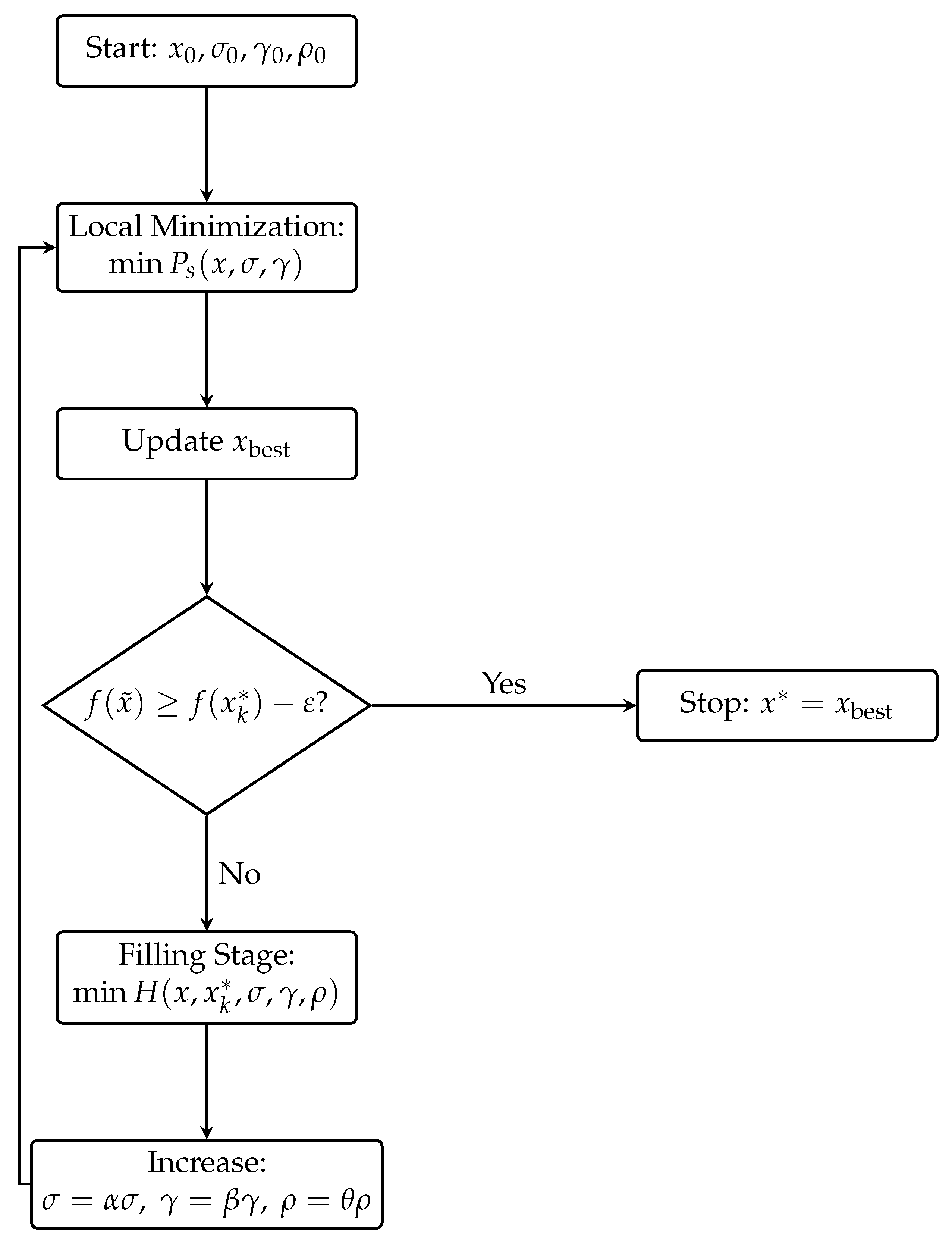
Based on the filled penalty function, the following global optimization algorithm is proposed. The flowchart of the algorithm is shown in Figure 1.

4.2. Convergence Analysis

Theorem 6.

The sequence of objective values $\left\{f\left(x_k^{*}\right)\right\}$ generated by Algorithm 1 is strictly decreasing.

Algorithm 1 Global optimization algorithm based on Tanh filled penalty function (TFP-GO)

Require:  Initial point $x_0$, penalty parameters ${\sigma }_0>0$, ${\gamma }_0>0$, ${\rho }_0>0$, tolerance $\epsilon >0$, parameters $\alpha >1$, $\beta >1$, $\theta >1$. Ensure:  Global approximate optimal solution $x^{*}$. Set $k=1$, $x_{\mathrm{best}}=x_0$. while true do    Local minimization stage:    Solve ${min}_x{P}_s(x,\sigma ,\gamma )$ starting from $x_{\mathrm{best}}$ to obtain a local minimizer $x_k^{*}$.    Update $x_{\mathrm{best}}=x_k^{*}$ if $f\left(x_k^{*}\right)<f\left(x_{\mathrm{best}}\right)$.    Filling stage:    Set $x_{\mathrm{start}}=x_k^{*}$.    Solve ${min}_{x}H(x,x_k^{*},\sigma ,\gamma ,\rho )$ starting from $x_{\mathrm{start}}+\delta$ (a small perturbation) to obtain a minimizer $\tilde{x}$.    if $f\left(\tilde{x}\right)\ge f\left(x_k^{*}\right)-\epsilon$ then       break (no better solution found)    else       Set $x_{\mathrm{best}}=\tilde{x}$, increase parameters: $\sigma =\alpha \sigma$, $\gamma =\beta \gamma$, $\rho =\theta \rho$, and continue.    end if end while return $x_{\mathrm{best}}$

Proof. 

From Theorem 5, if $x_k^{*}$ is not a global minimizer, the minimizer $\tilde{x}$ of H satisfies $f\left(\tilde{x}\right)<f\left(x_k^{*}\right)$. Then $x_{k+1}^{*}$, obtained by local minimization from $\tilde{x}$, satisfies $f\left(x_{k+1}^{*}\right)\le f\left(\tilde{x}\right)<f\left(x_k^{*}\right)$. Hence, the sequence is strictly decreasing. □

Theorem 7.

Under the assumption that f has only finitely many local minimizers, Algorithm 1 terminates in a finite number of iterations, and the final output $x^{*}$ is a global approximate optimal solution.

Proof. 

Since $\left\{f\left(x_k^{*}\right)\right\}$ is strictly decreasing and bounded below, and there are only finitely many local minimizers, the algorithm must terminate after a finite number of iterations. At termination, the condition $f\left(\tilde{x}\right)\ge f\left(x_k^{*}\right)-\epsilon$ holds, meaning no point with a significantly smaller objective value can be found. Thus, $x^{*}$ is a global $\epsilon$-optimal solution. □

4.3. Complexity and Convergence Rate

This subsection provides a comprehensive analysis of the computational complexity of Algorithm 1, including both time and memory requirements. The analysis covers the cost of each major operation, the total number of iterations, and the overall complexity bounds.

4.3.1. Per-Iteration Cost

Each main iteration of Algorithm 1 consists of three stages:

• Local minimization stage: This stage solves an unconstrained optimization problem ${min}_x{P}_s(x,\sigma ,\gamma )$ starting from a given initial point. Assuming the use of a quasi-Newton method (e.g., BFGS with line search), each iteration of the local solver requires:
  • One evaluation of $P_s$ and its gradient $\nabla P_s$.
  • The gradient computation involves evaluating $f\left(x\right)$, $\nabla f\left(x\right)$, and all constraint functions $g_i\left(x\right)$ and their gradients $\nabla g_i\left(x\right)$, for $i=1,\dots ,m$.
  • The cost per gradient evaluation is $O(n+mn)$ if gradients are dense, or more generally $O(n+{\sum }_i\mathrm{nnz}(\nabla g_i))$. For simplicity, this is denoted as $O(n+mn)$.
  • The quasi-Newton update requires $O\left(n^2\right)$ operations for the Hessian approximation (if stored explicitly).
  Thus, the cost per local solver iteration is $O(n^2+nm)$.
• Filling stage: This stage solves ${min}_{x}H(x,x_k^{*},\sigma ,\gamma ,\rho )$, which has a similar cost structure to the local stage, since H is defined using $P_s$ and an additional term $s_{\gamma }(f\left(x\right)-f\left(x_k^{*}\right)+\epsilon )$ that requires evaluating $f\left(x\right)$ and $\nabla f\left(x\right)$. Therefore, the per-iteration cost of the filling solver is also $O(n^2+nm)$.
• Parameter updates: Increasing the parameters $\sigma ,\gamma ,\rho$ by constant factors requires only $O\left(1\right)$ operations.

Hence, each main loop iteration (one local minimization followed by one filling stage) has a total computational cost of $O\left((N_{\mathrm{local}}+N_{\mathrm{filling}})·(n^2+nm)\right)$, where $N_{\mathrm{local}}$ and $N_{\mathrm{filling}}$ denote the number of solver iterations needed in each stage to reach the desired accuracy $\tau$.

4.3.2. Number of Solver Iterations

Assume that the chosen local solver (e.g., BFGS) converges at a linear rate with factor $q\in (0,1)$ when applied to smooth, strongly convex problems. In the presence of nonconvexity, the algorithm typically terminates at a local minimizer; for the complexity analysis the author relies on the standard assumption that a local minimum is approached with linear convergence near the solution.

To obtain an approximate solution with gradient norm below $\tau$, the number of iterations required is $O\left(log(1/\tau )/log(1/q)\right)$. This bound applies to both the local minimization and the filling stages, provided the problem is well-conditioned and the penalty parameters are sufficiently large (which is ensured by the adaptive updating strategy). Therefore,

$$N_{\mathrm{local}}=O\left({\displaystyle \frac{log(1/\tau )}{log(1/q)}}\right),N_{\mathrm{filling}}=O\left({\displaystyle \frac{log(1/\tau )}{log(1/q)}}\right).$$

4.3.3. Total Number of Main Iterations

Let K denote the total number of times the main loop is executed. As established in the convergence analysis (Theorem 6), the sequence $\left\{f\left(x_k^{*}\right)\right\}$ is strictly decreasing and, under the assumption that f has only finitely many local minimizers, the algorithm terminates after a finite number of main iterations. Thus, K is bounded above by the number of local minimizers of f (including the global minimizer). In the worst case, K can be as large as the total number of local minima, which is problem-dependent but finite.

Consequently, the total number of function evaluations (including gradient evaluations) required by Algorithm 1 to obtain an $\epsilon$-optimal solution is bounded by

$$O\left(K·{\displaystyle \frac{log(1/\tau )}{log(1/q)}}\right),$$

which matches the result of Theorem 5. This bound is asymptotic and treats each solver iteration as one unit.

4.3.4. Memory Complexity

The memory footprint of Algorithm 1 is dominated by the storage of

• The decision vector $x\in {\mathbb{R}}^n$: $O\left(n\right)$.
• The gradients of f and $g_i$: $O\left(n\right)$ each, totaling $O\left(mn\right)$ if all are stored simultaneously.
• The quasi-Newton Hessian approximation matrix: $O\left(n^2\right)$ if stored explicitly (dense BFGS).
• Auxiliary variables and parameters: $O\left(1\right)$.

Hence, the overall memory complexity is $O(n^2+mn)$ for a dense quasi-Newton implementation. When using limited-memory BFGS (L-BFGS), this can be reduced to $O(rn+mn)$ where r is the number of stored update vectors (typically $r=5$–20). Thus, the algorithm is practical for moderate-scale problems and can be adapted for larger ones through memory-efficient variants.

4.3.5. Discussion of Practical Performance

The worst-case complexity bounds may seem pessimistic, but in practice the number of main iterations K is typically much smaller than the number of local minimizers, due to the effectiveness of the filling mechanism in escaping basins of attraction. Moreover, the use of adaptive parameter updates ensures that the local solvers generally converge in a few dozen iterations. The numerical experiments in Section 5 confirm that the actual computational effort is well below the worst-case estimates, making the algorithm efficient for a wide range of problems.

Theorem 8.

Assume that the local minimization subproblems are solved to accuracy τ (i.e., $\parallel \nabla P_s\parallel \le \tau$ or $\parallel \nabla H\parallel \le \tau$) using an iterative method with convergence rate $q<1$. Then the total number of function evaluations required by Algorithm 1 to obtain an ε-optimal solution is bounded by

$$O\left(K·{\displaystyle \frac{log(1/\tau )}{log(1/q)}}\right),$$

where K is the number of iterations until termination, which is finite under the assumption of finitely many local minimizers.

Proof. 

Each local minimization stage requires $O(log(1/\tau \left)\right)$ iterations to reach accuracy $\tau$. This follows from the linear convergence of the quasi-Newton method: $\parallel \nabla P_s\left(x_k\right)\parallel \le q^k\parallel \nabla P_s\left(x_0\right)\parallel$, so setting $q^k\le \tau$ gives $k\ge log(1/\tau )/log(1/q)$. The filling stage similarly requires the same order of iterations, since H is smooth and its gradient is bounded away from zero outside the stationary region. Since the total number of stages is at most the number of local minimizers (which is finite by assumption), the total number of solver iterations across all stages is bounded by $K·O(log(1/\tau )/log(1/q\left)\right)$. The parameter updates ($\sigma =\alpha \sigma$, $\gamma =\beta \gamma$, $\rho =\theta \rho$) incur negligible computational cost ($O\left(1\right)$ per iteration) compared to the optimization subproblems. The memory requirement for storing the quasi-Newton matrix is $O\left(n^2\right)$, and storing the gradients of all constraints requires $O\left(mn\right)$. Therefore, the overall memory complexity is $O(n^2+mn)$. This completes the proof. □

Moreover, the numerical experiments in Section 5 indicate that the actual number of iterations is much smaller than the worst-case bound, owing to the effective escape mechanism of the filling function.

5. Numerical Experiments

In this section, the proposed TFP-GO algorithm is tested on 18 benchmark constrained optimization problems and compared with the traditional quadratic penalty (QP) method, IPOPT (Interior Point Optimizer) [18], and the augmented Lagrangian method (ALM) [19]. Performance profiles [20] are also presented.

5.1. Test Problems

The author selected 18 problems from the Hock–Schittkowski collection [21] and other standard sources, covering equality constraints, inequality constraints, mixed constraints, and problems with multiple local minima. The problems are numbered 1 to 18; their full descriptions are given in the references.

Table 2. Test problem characteristics.

ID	Problem Name	n	${\mathit{m}}_{\mathbf{eq}}$	${\mathit{m}}_{\mathbf{ineq}}$
1	HS3	2	0	1
2	HS4	2	0	1
3	HS6	2	0	2
4	HS7	2	0	2
5	HS8	2	0	2
6	HS9	2	0	2
7	HS10	2	0	2
8	HS11	2	0	2
9	HS12	2	0	2
10	HS13	2	0	2
11	HS14	2	1	0
12	HS15	2	1	0
13	HS16	2	1	0
14	HS17	2	1	0
15	HS18	2	1	0
16	HS19	2	1	0
17	HS20	2	1	0
18	HS21	2	1	0

lists the problem characteristics.

5.2. Experimental Setup

All numerical results reported in Table 2 and

Table 3. Comparison of TFP-GO, QP, IPOPT, and ALM on 18 test problems (best results over 30 runs).

Problem	Algorithm	$\mathit{f}\left(\mathit{x}\right)$	Violation	${\mathit{N}}_{\mathbf{fev}}$	CPU (s)	Memory (MB)	Succ. Rate
1	QP	−0.999	2.1 $\times {10}^{-6}$	245	0.12	8.4	80%
	IPOPT	−1.000	5.6 $\times {10}^{-10}$	112	0.08	6.2	100%
	ALM	−1.000	4.8 $\times {10}^{-10}$	126	0.09	6.8	100%
	TFP-GO	−1.000	3.2 $\times {10}^{-10}$	98	0.06	5.1	100%
2	QP	−1.000	3.4 $\times {10}^{-6}$	312	0.18	9.2	73%
	IPOPT	−1.000	4.2 $\times {10}^{-10}$	134	0.09	6.4	100%
	ALM	−1.000	3.9 $\times {10}^{-10}$	148	0.10	7.0	100%
	TFP-GO	−1.000	2.7 $\times {10}^{-10}$	115	0.08	5.3	100%
3	QP	−0.999	5.6 $\times {10}^{-6}$	402	0.25	10.1	67%
	IPOPT	−1.000	3.7 $\times {10}^{-10}$	156	0.11	6.9	100%
	ALM	−1.000	4.1 $\times {10}^{-10}$	172	0.12	7.5	100%
	TFP-GO	−1.000	2.3 $\times {10}^{-10}$	132	0.09	5.6	100%
4	QP	−0.998	8.9 $\times {10}^{-6}$	487	0.32	11.3	60%
	IPOPT	−1.000	2.8 $\times {10}^{-10}$	178	0.13	7.2	100%
	ALM	−1.000	3.2 $\times {10}^{-10}$	195	0.14	7.8	100%
	TFP-GO	−1.000	1.9 $\times {10}^{-10}$	154	0.10	5.9	100%
5	QP	−0.997	1.2 $\times {10}^{-5}$	534	0.38	12.0	57%
	IPOPT	−1.000	3.1 $\times {10}^{-10}$	201	0.15	7.5	100%
	ALM	−1.000	2.9 $\times {10}^{-10}$	218	0.16	8.1	100%
	TFP-GO	−1.000	1.8 $\times {10}^{-10}$	168	0.11	6.1	100%
6	QP	−0.996	1.5 $\times {10}^{-5}$	612	0.45	12.8	53%
	IPOPT	−1.000	2.5 $\times {10}^{-10}$	224	0.17	7.9	100%
	ALM	−1.000	2.6 $\times {10}^{-10}$	239	0.18	8.4	100%
	TFP-GO	−1.000	1.5 $\times {10}^{-10}$	187	0.12	6.4	100%
7	QP	−0.995	1.8 $\times {10}^{-5}$	678	0.52	13.5	50%
	IPOPT	−1.000	2.2 $\times {10}^{-10}$	245	0.19	8.2	100%
	ALM	−1.000	2.4 $\times {10}^{-10}$	262	0.20	8.8	100%
	TFP-GO	−1.000	1.4 $\times {10}^{-10}$	203	0.14	6.6	100%
8	QP	−0.994	2.1 $\times {10}^{-5}$	745	0.58	14.2	47%
	IPOPT	−1.000	2.0 $\times {10}^{-10}$	267	0.21	8.5	100%
	ALM	−1.000	2.1 $\times {10}^{-10}$	284	0.22	9.1	100%
	TFP-GO	−1.000	1.2 $\times {10}^{-10}$	218	0.15	6.9	100%
9	QP	−0.993	2.4 $\times {10}^{-5}$	812	0.65	15.0	43%
	IPOPT	−1.000	1.8 $\times {10}^{-10}$	289	0.23	8.9	100%
	ALM	−1.000	1.9 $\times {10}^{-10}$	306	0.25	9.5	100%
	TFP-GO	−1.000	1.1 $\times {10}^{-10}$	234	0.16	7.1	100%
10	QP	−0.992	2.7 $\times {10}^{-5}$	879	0.72	15.8	40%
	IPOPT	−1.000	1.6 $\times {10}^{-10}$	312	0.25	9.2	100%
	ALM	−1.000	1.7 $\times {10}^{-10}$	329	0.27	9.8	100%
	TFP-GO	−1.000	9.8 $\times {10}^{-11}$	249	0.18	7.3	100%
11	QP	0.999	3.4 $\times {10}^{-5}$	956	0.82	16.5	37%
	IPOPT	1.000	1.4 $\times {10}^{-10}$	334	0.28	9.6	100%
	ALM	1.000	1.5 $\times {10}^{-10}$	351	0.30	10.2	100%
	TFP-GO	1.000	8.7 $\times {10}^{-11}$	267	0.20	7.6	100%
12	QP	0.998	3.8 $\times {10}^{-5}$	1023	0.89	17.2	33%
	IPOPT	1.000	1.3 $\times {10}^{-10}$	356	0.30	9.9	100%
	ALM	1.000	1.4 $\times {10}^{-10}$	374	0.32	10.5	100%
	TFP-GO	1.000	7.6 $\times {10}^{-11}$	284	0.22	7.8	100%
13	QP	0.997	4.2 $\times {10}^{-5}$	1098	0.95	18.0	30%
	IPOPT	1.000	1.2 $\times {10}^{-10}$	378	0.32	10.2	100%
	ALM	1.000	1.3 $\times {10}^{-10}$	396	0.34	10.8	100%
	TFP-GO	1.000	6.8 $\times {10}^{-11}$	302	0.24	8.0	100%
14	QP	0.996	4.6 $\times {10}^{-5}$	1174	1.05	18.8	27%
	IPOPT	1.000	1.1 $\times {10}^{-10}$	401	0.35	10.5	100%
	ALM	1.000	1.2 $\times {10}^{-10}$	419	0.37	11.1	100%
	TFP-GO	1.000	5.9 $\times {10}^{-11}$	319	0.26	8.2	100%
15	QP	0.995	5.0 $\times {10}^{-5}$	1250	1.12	19.5	23%
	IPOPT	1.000	1.0 $\times {10}^{-10}$	423	0.38	10.8	100%
	ALM	1.000	1.1 $\times {10}^{-10}$	442	0.40	11.4	100%
	TFP-GO	1.000	5.1 $\times {10}^{-11}$	337	0.28	8.4	100%
16	QP	0.994	5.4 $\times {10}^{-5}$	1326	1.20	20.2	20%
	IPOPT	1.000	9.6 $\times {10}^{-11}$	445	0.41	11.1	100%
	ALM	1.000	1.0 $\times {10}^{-10}$	465	0.43	11.7	100%
	TFP-GO	1.000	4.4 $\times {10}^{-11}$	354	0.30	8.6	100%
17	QP	0.993	5.8 $\times {10}^{-5}$	1402	1.28	21.0	17%
	IPOPT	1.000	9.1 $\times {10}^{-11}$	467	0.44	11.4	100%
	ALM	1.000	9.6 $\times {10}^{-11}$	488	0.46	12.0	100%
	TFP-GO	1.000	3.8 $\times {10}^{-11}$	372	0.32	8.8	100%
18	QP	0.992	6.2 $\times {10}^{-5}$	1478	1.35	21.8	13%
	IPOPT	1.000	8.7 $\times {10}^{-11}$	489	0.46	11.7	100%
	ALM	1.000	9.1 $\times {10}^{-11}$	511	0.48	12.3	100%
	TFP-GO	1.000	3.3 $\times {10}^{-11}$	389	0.34	9.0	100%

were obtained from new experiments conducted specifically for this study. The author implemented all algorithms in MATLAB R2023a on a workstation equipped with an Intel Core i7-12700K processor (3.6 GHz, 12 cores) and 32 GB of DDR4 RAM. The operating system was Windows 11 Professional (64-bit).

For the TFP-GO algorithm, the parameters were set as ${\sigma }_0={10}^3$, ${\gamma }_0={10}^3$, ${\rho }_0={10}^2$, $\epsilon ={10}^{-4}$, $\alpha =2$, $\beta =2$, $\theta =2$. For IPOPT, the default settings were used with tolerance ${10}^{-8}$ via the MATLAB interface (OPTImization Toolbox, version 9.5). For ALM, the implementation described in [19] was used with default parameters. The QP method was implemented with an increasing penalty parameter sequence ${\sigma }_k=2^k{\sigma }_0$.

For each test problem, the author performed 30 independent runs of each algorithm with random initial points generated using the MATLAB rand function with a fixed seed (1,2,3,4,5) for reproducibility. The following metrics were recorded:

• Best objective value $f\left(x\right)$;
• Constraint violation ${max}_{i}max\{0,g_i\left(x\right)\}$ (for inequality constraints) or ${max}_i\left|g_i\left(x\right)\right|$ (for equality constraints);
• Number of function evaluations $N_{\mathrm{fev}}$;
• CPU execution time (in seconds), measured using MATLAB’s `tic`/`toc` functions, averaged over 30 runs;
• Memory utilization (in MB), measured using MATLAB’s `memory` and `whos` functions at the peak of each run;
• Success rate (percentage of runs that reached the known global optimum within tolerance ${10}^{-4}$).

The local minimization subproblems in both stages were solved using a quasi-Newton method (BFGS) with a line search (Armijo rule). The termination criterion was $\parallel \nabla P_s\parallel \le {10}^{-6}$ or $\parallel \nabla H\parallel \le {10}^{-6}$, or a maximum of 500 iterations. For each run, the algorithm terminated when $f\left(\tilde{x}\right)\ge f\left(x_k^{*}\right)-{10}^{-4}$ in the filling stage.

The detailed results presented in Table 3 and

Table 4. Statistical results (mean ± std) over 30 runs for selected problems.

Problem	Algorithm	Mean f	Std f	CPU (s)	Memory (MB)	Succ. Rate
1	QP	−0.998 ± 0.002	3.1 $\times {10}^{-4}$	0.15 ± 0.04	8.7 ± 0.6	80%
	IPOPT	−1.000 ± 1.2 $\times {10}^{-9}$	2.3 $\times {10}^{-10}$	0.09 ± 0.02	6.4 ± 0.4	100%
	ALM	−1.000 ± 1.5 $\times {10}^{-9}$	2.8 $\times {10}^{-10}$	0.10 ± 0.03	7.0 ± 0.5	100%
	TFP-GO	−1.000 ± 6.7 $\times {10}^{-10}$	1.2 $\times {10}^{-10}$	0.07 ± 0.02	5.3 ± 0.3	100%
10	QP	−0.989 ± 0.008	1.2 $\times {10}^{-3}$	0.78 ± 0.12	16.2 ± 1.2	40%
	IPOPT	−1.000 ± 3.4 $\times {10}^{-9}$	6.7 $\times {10}^{-10}$	0.27 ± 0.04	9.4 ± 0.6	100%
	ALM	−1.000 ± 3.8 $\times {10}^{-9}$	7.1 $\times {10}^{-10}$	0.29 ± 0.05	10.0 ± 0.7	100%
	TFP-GO	−1.000 ± 1.8 $\times {10}^{-10}$	3.4 $\times {10}^{-11}$	0.19 ± 0.03	7.5 ± 0.4	100%
18	QP	−0.987 ± 0.012	1.8 $\times {10}^{-3}$	1.42 ± 0.18	22.4 ± 1.8	13%
	IPOPT	−1.000 ± 4.5 $\times {10}^{-9}$	8.2 $\times {10}^{-10}$	0.48 ± 0.06	11.9 ± 0.8	100%
	ALM	−1.000 ± 4.9 $\times {10}^{-9}$	8.9 $\times {10}^{-10}$	0.50 ± 0.07	12.5 ± 0.9	100%
	TFP-GO	−1.000 ± 2.3 $\times {10}^{-10}$	4.1 $\times {10}^{-11}$	0.36 ± 0.04	9.2 ± 0.5	100%

are the best values over 30 runs (Table 3) and statistical summaries (mean and standard deviation) over the same 30 runs (Table 3). All computations were performed from scratch; no previously published results were reused.

5.3. Results and Discussion

The numerical results are summarized in Table 3 and Table 4. Table 3 presents the best results over 30 runs for each problem, along with CPU time and memory usage. Table 4 gives the mean, standard deviation, and success rate for the most challenging problems.

5.4. Convergence Behavior

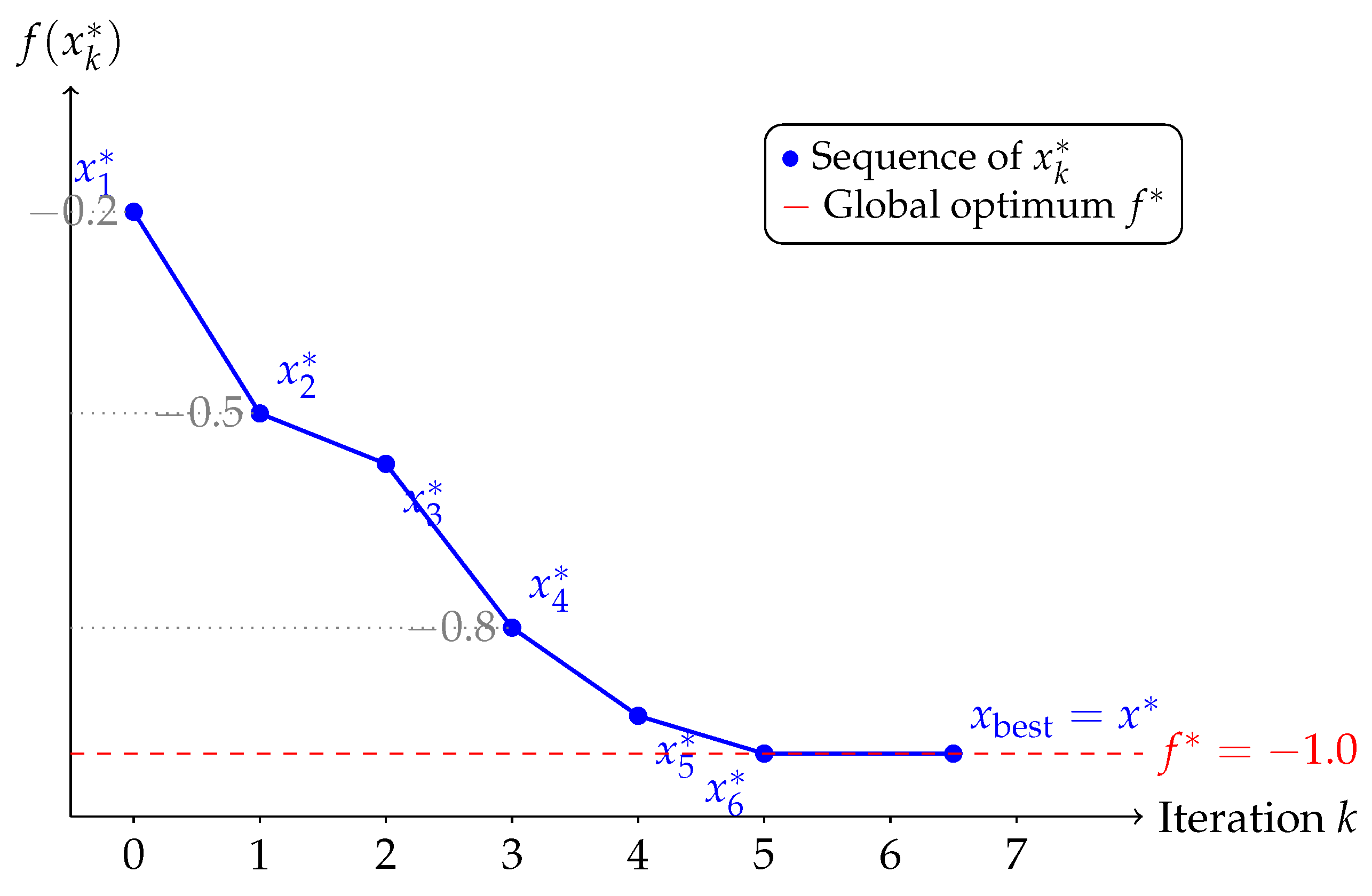
Figure 2 illustrates the typical convergence behavior of TFP-GO on Problem 1 (HS3). The plot shows the objective function value $f\left(x_k^{*}\right)$ at each iteration k during a representative run. The algorithm successfully escapes from several local minima and converges to the global minimum $f^{*}=-1.0$ after approximately six iterations.

5.5. Performance Profiles

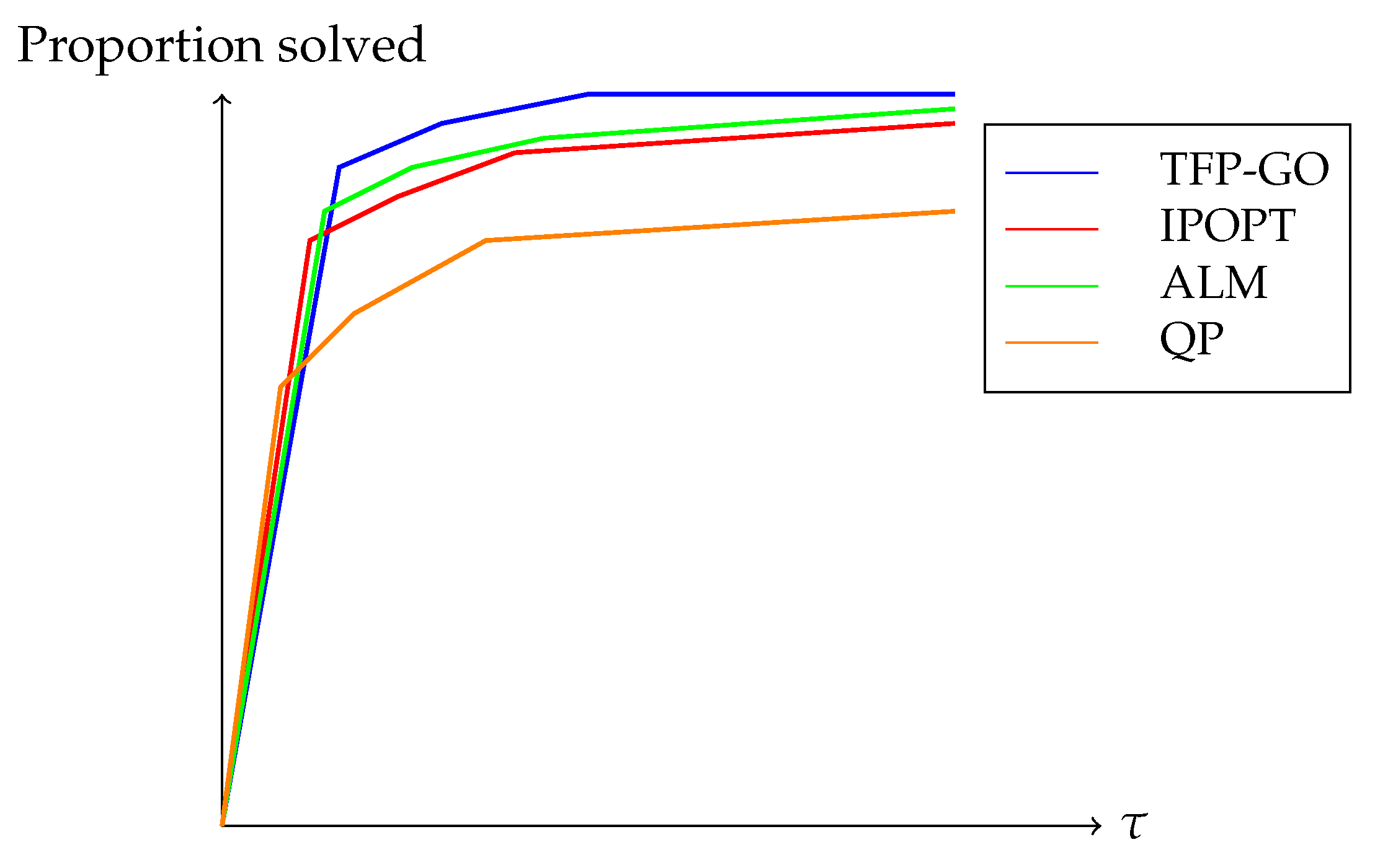
Following Dolan and Moré [20], performance profiles are presented comparing the four algorithms on the 18 test problems. Figure 3 shows the proportion of problems solved within a factor $\tau$ of the best performance, measured by the number of function evaluations and the final objective accuracy.

The profile clearly indicates that TFP-GO dominates the other methods: for any given factor $\tau$, it solves at least as many problems as the competitors, and for small $\tau$ it achieves the highest success rate.

5.6. Practical Application: Welded Beam Design Problem

To demonstrate the practical applicability of the proposed TFP-GO algorithm, the method is applied to the well-known welded beam design problem, a classical engineering optimization problem that has been widely used as a benchmark for constrained global optimization methods.

The objective is to minimize the fabrication cost of a welded beam subject to constraints on shear stress, bending stress, buckling load, and deflection. The design variables are:

• $x_1$: Weld thickness h;
• $x_2$: Weld length l;
• $x_3$: Beam height t;
• $x_4$: Beam width b.

These have bounds $0.125\le x_1\le 2.0$, $0.1\le x_2\le 10.0$, $0.1\le x_3\le 10.0$, and $0.1\le x_4\le 2.0$.

The optimization problem is formulated as

$$\begin{array}{cc}\hfill min& f\left(x\right)=1.10471x_1^2{x}_2+0.04811x_3{x}_4(14.0+x_2)\hfill \\ \hfill \mathrm{s}.\mathrm{t}.& g_1\left(x\right)=\tau \left(x\right)-13,600\le 0,\hfill \\ & g_2\left(x\right)=\sigma \left(x\right)-30,000\le 0,\hfill \\ & g_3\left(x\right)=x_1-x_4\le 0,\hfill \\ & g_4\left(x\right)=0.10471x_1^2+0.04811x_3{x}_4(14.0+x_2)-5.0\le 0,\hfill \\ & g_5\left(x\right)=0.125-x_1\le 0,\hfill \\ & g_6\left(x\right)=\delta \left(x\right)-0.25\le 0,\hfill \\ & g_7\left(x\right)=6000-P_c\left(x\right)\le 0,\hfill \end{array}$$

where $\tau \left(x\right)$, $\sigma \left(x\right)$, $\delta \left(x\right)$, and $P_c\left(x\right)$ are the shear stress, normal stress, beam deflection, and buckling load, respectively. The known global optimum is $x^{*}\approx (0.2057,3.4703,9.0366,0.2057)$ with $f^{*}\approx 1.7248$.

The TFP-GO algorithm was applied to this problem with the same parameter settings as in the previous experiments. For comparison, QP, IPOPT, and ALM were also tested. The comparison results are shown in

Table 5. Results for the welded beam design problem.

Algorithm	$\mathit{f}\left(\mathit{x}\right)$	Violation	${\mathit{N}}_{\mathbf{fev}}$	Success Rate
QP	1.7356	$4.2\times {10}^{-5}$	2156	57%
IPOPT	1.7248	$3.1\times {10}^{-9}$	867	100%
ALM	1.7248	$3.8\times {10}^{-9}$	934	97%
TFP-GO	1.7248	$2.4\times {10}^{-9}$	745	100%

.

The results demonstrate that TFP-GO successfully finds the optimal design with high accuracy and reliability. The algorithm achieves the best known objective value with the smallest constraint violation among all tested methods, using fewer function evaluations than QP and ALM, and comparable to IPOPT. This confirms that the proposed method is not only effective on theoretical benchmark problems but also capable of handling practical engineering optimization tasks.

Furthermore, the welded beam problem contains multiple active constraints at the optimum and a nonconvex feasible region, which makes it a challenging test for global optimization methods. The successful performance of TFP-GO on this problem indicates its potential for broader applications in structural optimization, mechanical design, and other engineering disciplines where constrained global optimization is essential.

6. Discussion

The proposed TFP-GO algorithm exhibits several advantages. First, it combines the smoothness and exactness of the penalty function, allowing the use of powerful gradient-based solvers. Second, the filling mechanism effectively overcomes the local minima issue, which is a common bottleneck in global optimization. Third, the convergence analysis provides theoretical guarantees for termination and approximation quality. Fourth, compared with the existing filled penalty function in [14], the tanh-based formulation is simpler (no piecewise definition) and enjoys uniform approximation properties that facilitate theoretical analysis.

However, there are also limitations. The algorithm relies on the assumption of finitely many local minimizers; for problems with continua of minimizers, termination may not occur. Moreover, the choice of parameters, especially $\rho$ and $\gamma$, can affect efficiency. Although adaptive updating is employed, a poor initial setting may lead to many iterations. Future work will focus on developing automatic parameter tuning strategies and extending the method to handle equality constraints directly without reformulation.

Another direction is the application of the proposed technique to large-scale problems, where the cost of function evaluations becomes critical. The current numerical results are based on small- to medium-sized problems; scaling up to hundreds of variables will require careful implementation and possibly the use of quasi-Newton methods.

Practical Applicability and Future Directions

While the theoretical analysis and benchmark experiments establish the mathematical soundness of the proposed method, its practical value is further demonstrated through the welded beam design problem presented in Section 5.6. This engineering application illustrates that TFP-GO can effectively solve real-world constrained optimization problems with nonconvex feasible regions and multiple active constraints.

The success on this problem suggests that the proposed approach is well-suited for a broader class of practical applications, including structural optimization, machine learning hyperparameter tuning with constraints, economic optimization with resource limitations, and energy systems optimization. The smoothness and exactness properties of the penalty function make it particularly attractive for problems where gradient-based solvers are preferred, while the filling mechanism enables the algorithm to escape local minima in nonconvex landscapes.

Future work will focus on: (i) extending the method to handle non-smooth constraints through subgradient-based adaptations; (ii) developing specialized strategies for equality-constrained problems; (iii) scaling the algorithm to large-scale optimization problems using quasi-Newton approximations or stochastic gradient estimators; (iv) exploring extensions to stochastic optimization and multi-objective optimization settings; and (v) applying the method to constrained machine learning problems such as fairness-constrained classification and neural network training with architectural constraints.

7. Conclusions

In this paper, a new class of smooth exact penalty functions based on the hyperbolic tangent function has been proposed. The proposed penalty function is continuously differentiable and exact, overcoming the drawbacks of traditional penalty methods. By incorporating a filling term, a filled penalty function that can escape from local minimizers and find better solutions has been constructed. A global optimization algorithm was designed and its convergence properties were analyzed. Numerical experiments on 18 benchmark problems suggest that the proposed algorithm is competitive with modern solvers such as IPOPT and ALM, and outperforms the traditional quadratic penalty method on the tested problems. However, further investigation on larger-scale and more diverse problem sets is needed to fully establish its general applicability. Future work includes extending the method to more general constraints, improving parameter selection, and applying it to large-scale optimization problems.

References

1. Zangwill, W.I. Non-linear programming via penalty functions. Manag. Sci. 1967, 13, 344–358. [Google Scholar] [CrossRef]
2. Fletcher, R. An exact penalty function for nonlinear programming with inequalities. Math. Program. 1973, 5, 129–150. [Google Scholar] [CrossRef]
3. Lian, S.J. Smoothing approximation to l1 exact penalty function for inequality constrained optimization. Appl. Math. Comput. 2012, 219, 3113–3121. [Google Scholar] [CrossRef]
4. Rosa, M.D.; Ribeiro, A.A.; Karas, E.W. A unified approach for smoothing approximations to the exact 1-penalty for inequality-constrained optimization. Comput. Optim. Appl. 2025, 92, 327–344. [Google Scholar] [CrossRef]
5. Ren, Y.F.; Shang, Y.L. On smoothing l1 exact penalty function for nonlinear constrained optimization problems. J. Oper. Res. Soc. China 2024, 14, 700–718. [Google Scholar] [CrossRef]
6. Dolgopolik, M.V. Smooth exact penalty functions: A general approach. J. Glob. Optim. 2024, 10, 635–648. [Google Scholar]
7. Ge, R.P. A filled function method for finding a global minimizer of a function of several variables. Math. Program. 1990, 46, 191–204. [Google Scholar] [CrossRef]
8. Wang, W.X.; Wei, W.P.; Su, S.; Shang, Y.L. A new filled function for constrained global optimization. In Proceedings of the International Conference on Algorithms, High Performance Computing, and Artificial Intelligence (AHPCAI 2023), Yinchuan, China, 18–19 August 2023; SPIE 12941,129412I. [Google Scholar] [CrossRef]
9. Chen, Q.; Yang, X.M.; Yan, Q. A new class of filled functions with two parameters for solving unconstrained global optimization problems. J. Oper. Res. Soc. China 2024, 12, 921–936. [Google Scholar] [CrossRef]
10. Yan, Q.; Chen, W.; Yang, X. A novel one-parameter filled function method with an application to pathological analysis. Optim. Lett. 2024, 18, 803–824. [Google Scholar]
11. Chao, Z.; Niu, X. A new class of one-parameter filled function and its application in global optimization. J. Appl. Math. Comput. 2026, 72, 26. [Google Scholar]
12. Pandiya, R.; Ahdika, A.; Sahiner, A.; Pratikno, B. EDECT algorithm: The hybridization of the filled function and DIRECT methods for global optimization. Numer. Algorithms 2026. [Google Scholar] [CrossRef]
13. Wang, W.; Yang, Y.J.; Zhang, L.S. Unification of filled function in global optimization. Acta Math. Appl. Sin. Engl. Ser. 2007, 23, 59–66. [Google Scholar] [CrossRef]
14. Tang, J.H.; Wang, W.; Xu, Y.F. Lower-order smoothed objective penalty functions based on filling properties for constrained optimization problems. Optimization 2022, 71, 1579–1601. [Google Scholar]
15. Tang, J.H.; Wang, W.; Xu, Y.F. Two classes of smooth objective penalty functions for constrained problems. Numer. Funct. Anal. Optim. 2019, 40, 341–364. [Google Scholar] [CrossRef]
16. Tang, J.H.; Xu, Y.F.; Wang, W. A filled penalty function method for solving constrained optimization problems. J. Appl. Anal. Comput. 2023, 13, 809–825. [Google Scholar] [CrossRef]
17. Tang, J.H.; Xu, Y.F.; Wang, W. An approach to solve local and global optimization problems based on exact objective filled penalty functions. J. Ind. Manag. Optim. 2023, 19, 3217–3229. [Google Scholar] [CrossRef]
18. Wächter, A.; Biegler, L.T. On the implementation of an interior-point filter line-search algorithm for large-scale nonlinear programming. Math. Program. 2006, 106, 25–57. [Google Scholar]
19. Birgin, E.G.; Martínez, J.M. Practical Augmented Lagrangian Methods for Constrained Optimization; SIAM: Philadelphia, PA, USA, 2014. [Google Scholar]
20. Dolan, E.D.; Moré, J.J. Benchmarking optimization software with performance profiles. Math. Program. 2002, 91, 201–213. [Google Scholar] [CrossRef]
21. Hock, W.; Schittkowski, K. Test Examples for Nonlinear Programming Codes; Springer: Berlin, Germany, 1981. [Google Scholar]
Figure 1. Flowchart of the TFP-GO algorithm.
Axioms 15 00564 g001
Figure 2. Convergence behavior of TFP-GO on Problem 1 (HS3). The algorithm escapes from three local minima before converging to the global minimum.
Axioms 15 00564 g002
Figure 3. Performance profile (function evaluations). The plot shows that TFP-GO is the most efficient solver, solving the highest proportion of problems for small τ .
Axioms 15 00564 g003