Noise-Adjusted Shrinkage Covariance Estimation in High Dimensions

Abstract

High-dimensional covariance estimation remains a fundamental challenge when the number of variables (p) substantially exceeds the sample size (n). In such settings, the sample covariance matrix is unstable, singular, and heavily contaminated by estimation noise. Although shrinkage estimators improve stability and thresholding methods promote sparsity, each approach alone may introduce bias or lose structural information. This study proposes a Noise-Adjusted Shrinkage Covariance (NASC) framework as a post-processing enhancement strategy for shrinkage-based covariance estimators. The framework first stabilizes the covariance structure through shrinkage toward a structured target, then suppresses noise-induced small covariance entries via thresholding, and finally applies a stabilization step to ensure positive definiteness of the resulting estimator. Sensitivity analyses were conducted to investigate the effects of the shrinkage and thresholding parameters, and the Monte Carlo simulations were subsequently performed using the best-performing parameter configuration. The simulation results showed that shrinkage alone may not sufficiently suppress entrywise noise, whereas NASC-adjusted estimators improved upon their corresponding shrinkage baselines in many scenarios, with the strongest gains observed for sparse covariance structures and for shrinkage estimators that do not explicitly suppress entrywise estimation noise. Improvements were more limited for highly optimized shrinkage estimators. Real-data analyses were conducted on the SRBCT and colon cancer benchmark datasets. On the SRBCT dataset, numerical stability and positive-definiteness properties were examined, while LOOCV-LDA classification performance without prior feature selection or dimensionality reduction was evaluated on the colon cancer dataset. The results suggest that NASC provides a computationally simple and numerically stable extension to classical shrinkage covariance estimation methods for high-dimensions.

1. Introduction

In multivariate statistics, the sample covariance matrix $\left(S\right)$ is central to many fundamental methods such as dimensionality reduction, classification, portfolio optimization, and multivariate hypothesis testing. However, in the high-dimensional regime where the number of variables $\left(p\right)$ is much larger than the number of observations $\left(n\right)$ $(n\ll p)$, the classical sample covariance matrix $S$ becomes both numerically unstable (often singular/ill-conditioned) and a high-variance estimator; this directly undermines the reliability of subsequent analyses (inversion, discriminant analysis, correlation-based network inference, etc.).

Ledoit and Wolf’s work on large-dimensional covariance estimation highlighted the practical implications of the high-dimensional ill-conditioning of $S$, clearly demonstrating the need for well-conditioned estimators [1]. The idea of regularization in covariance estimation is rooted in the observation that sample eigenvalues systematically appear “overspread” (large values appear too large, small values too small). This observation is one of the starting points for Stein’s approach to estimating the covariance matrix (particularly the line that developed around his 1975 Rietz lectures) [2,3]. From this perspective, shrinkage methods pull the covariance structure towards a target structure to make it more stable; thus, the estimation variance is reduced and the invertibility/conditionality of the matrix is improved [4]. However, shrinkage often produces a dense covariance matrix: a large number of covariance inputs remain, though very small in size. Yet, in high-dimensional data, especially in many applications, it is often accepted that the covariance structure can be approximately sparse (or “most small inputs are at the noise level”).

A key line that directly utilizes this intuition is to regularize the covariance matrix through thresholding. Bickel and Levina provided a strong theoretical basis for the thresholding approach by showing that the covariance estimator obtained by input-based hard thresholding can be consistent in the operator norm under appropriate sparsity assumptions and under the condition ${\displaystyle \frac{logp}{n}}\to 0$ [5]. Later, Cai and Liu proposed adaptive thresholding that takes into account the variability of each covariance input, showing that universal (single-threshold) approaches can remain suboptimal in some classes and that adaptive procedures can achieve better convergence rates [6]. While thresholding methods simplify interpretation by eliminating small covariances, two practical challenges arise when used alone:

(i) The selection of the “noise threshold” is sensitive because the input-based estimation error can grow in the $n\ll p$ regime;

(ii) Naive thresholding can, in some cases, compromise fundamental structural properties such as positive definiteness.

Therefore, sparsity-based covariance estimation has also been studied through penalized regularization approaches. Lam and Fan (2009) investigated sparsistency and convergence properties for large covariance and precision matrix estimation [7]. Furthermore, Rothman, Levina, and Zhu (2009) proposed generalized thresholding operators that combine shrinkage and thresholding behaviors in a unified framework [8]. In addition, the POET approach introduced a low-rank plus sparse decomposition framework for high-dimensional covariance estimation [9]. More recently, shrinkage-based covariance estimation has continued to evolve through nonlinear shrinkage methods, structured targets, and data-driven shrinkage intensities [10,11,12,13]. These developments further highlight the importance of shrinkage for stabilizing covariance estimation in high-dimensional settings.

A second active research direction concerns the development of structured covariance estimators that combine shrinkage with additional structural constraints such as banding, tapering, or sparsity. These approaches aim to exploit prior knowledge about dependence patterns (e.g., locality, approximate sparsity, or structured correlation decay). For example, recent work has explored structured shrinkage toward banded or Toeplitz-type targets as well as hybrid estimators that combine shrinkage with tapering or thresholding mechanisms to improve performance under various covariance structures [14,15].

Third, modern research has increasingly emphasized theoretical guarantees and statistical inference in high-dimensional covariance models. Recent studies have investigated projection-based inference, structured shrinkage toward nonparametric covariance estimators, and improved estimation procedures under complex dependence structures [16]. These developments reflect a broader trend in high-dimensional statistics toward combining multiple regularization principles to achieve both statistical efficiency and structural interpretability.

Despite these advances, an important practical tension remains between two widely used regularization strategies. Shrinkage methods are primarily designed to stabilize the global spectral structure of the covariance matrix, while thresholding methods aim to remove small entrywise covariances that are likely to arise from sampling noise. In many high-dimensional applications, however, these two sources of estimation difficulty coexist: the sample covariance matrix is simultaneously spectrally unstable and artificially dense due to noise-level correlations. Consequently, methods that address only one of these issues may remain suboptimal.

Motivated by this observation, this study proposes a hybrid covariance estimation strategy that integrates shrinkage-based stabilization, entrywise thresholding, and positive-definite stabilization within a unified framework. The central idea is to first reduce the estimation variance through shrinkage toward a structured target matrix (such as the identity matrix or a diagonal matrix, which serves as a stable reference toward which the sample covariance matrix is shrunk), then apply thresholding to eliminate small covariance entries and, finally perform a stabilization step to ensure that the resulting covariance estimator remains positive definite and numerically well-conditioned. The aim of this study is to evaluate whether this sequential shrinkage–thresholding–stabilization framework can improve existing shrinkage covariance estimators under different high-dimensional regimes.

The remainder of this paper is organized as follows. Section 2 reviews the theoretical background of high-dimensional covariance estimation, summarizes existing shrinkage and thresholding approaches and, introduces the proposed NASC framework and describes its construction. Section 3 presents the sensitivity analyses used for parameter selection, reports the Monte Carlo simulation study, evaluates the performance of the proposed framework under different covariance structures and dimensionality settings, and illustrates its practical applicability using real high-dimensional datasets. Finally, Section 4 concludes the paper and discusses potential directions for future research.

2. Materials and Methods

2.1. What Fails in High Dimensions?

In high-dimensional undersized datasets ($n\ll p$) the sample covariance matrix $S$ loses much of its classical “well-behaved” properties, directly undermining the reliability of numerous multivariate methods. The fundamental problem is, when ($n\ll p$), $S$ becomes singular and irreversible. Even if $p$ and $n$ are of the same order, $S$ is often ill-conditioned, and the inversion operation dramatically increases the estimation error. Therefore, analyses based on $S$, such as regression, classification, dimension reduction, portfolio optimization, and graphical inference, either become technically impractical or are excessively sensitive to small sample fluctuations [17,18]. However, at high dimensions, there is not only a “numerical stability” problem; a second breakdown emerges: $S$ appears artificially dense due to noise accumulation; numerous small covariance inputs reflect sample noise, not actually a weak/insignificant relationship. Therefore, the input-based thresholding approach, especially under approximate sparsity, offers consistent prediction guarantees in the operator norm by suppressing small inputs (e.g., under condition ${\displaystyle \frac{logp}{n}}\to 0$) [5,6].

In summary, what fails at a high level is not just the singularity of $S$; it is simultaneously (i) spectral distortion/instability and (ii) the accumulation of spurious small correlations caused by noise [19]. This dual breakdown is the fundamental starting point that explains why methods using shrinkage alone or thresholding alone can systematically remain suboptimal in certain data structures.

2.2. Two Distinct Sources of Estimation Error

To formally characterize the sources of estimation error in high-dimensional covariance estimation, we first introduce basic notation and the statistical framework used throughout the paper.

Let $X_1,{\dots ,X}_nϵ {\mathbb{R}}^p$ denote independent observations of a $p$-dimensional random vector $X={(X_1,{\dots ,X}_p)}^T$, where $p$ represents the number of variables and $n$ the sample size. The mean vector is $\mu =E\left[X_i\right]$ and population covariance matrix is defined as

$$\mathsf{\Sigma }=E\left[\left(X_i-\mu \right){\left(X_i-\mu \right)}^T\right]$$

(1)

The classical estimator of $\mathsf{\Sigma }$ is the sample covariance matrix:

$$\mathrm{S}={\displaystyle \frac{1}{n}}{\displaystyle \sum _{i=1}^n}\left(X_i-\overline{X}\right){\left(X_i-\overline{X}\right)}^T$$

(2)

where $\overline{X}$ denotes the sample mean vector. To evaluate the accuracy of a covariance estimator $\widehat{\mathsf{\Sigma }},$ we measure estimation error using the Frobenius norm:

$${‖\widehat{\mathsf{\Sigma }}-\mathsf{\Sigma }‖}_F^2={\displaystyle \sum _{i=1}^p}{\displaystyle \sum _{j=1}^p}{\left({\widehat{\sigma }}_{ij}-{\sigma }_{ij}\right)}^2$$

(3)

The Frobenius norm measures the overall discrepancy between two matrices by aggregating the squared values of all matrix entries.

The estimation error of a covariance estimator $\widehat{\mathsf{\Sigma }}$ can be decomposed into two components that reflect different sources of uncertainty. Specifically,

$$\widehat{\mathsf{\Sigma }}-\mathsf{\Sigma }=\underset{Stochasticcomponent}{\underbrace{\left(\widehat{\mathsf{\Sigma }}-E\left[\widehat{\mathsf{\Sigma }}\right]\right)}}+\underset{structuralcomponenet}{\underbrace{(E\left[\widehat{\mathsf{\Sigma }}\right]-\mathsf{\Sigma })}}$$

(4)

$$\begin{gathered} E{‖\widehat{\mathsf{\Sigma }}-\mathsf{\Sigma }‖}_F^2=\mathrm{E}{‖\widehat{\mathsf{\Sigma }}-E\left[\widehat{\mathsf{\Sigma }}\right]‖}_F^2+{E‖E\left[\widehat{\mathsf{\Sigma }}\right]-\mathsf{\Sigma }‖}_F^2 \\ MSE=Variance+{Bias}^2 \end{gathered}$$

(5)

In high-dimensional settings the variance component of the sample covariance matrix increases rapidly with the dimension. In fact, the Frobenius risk of the sample covariance matrix grows on the order of

$${E‖S-\mathsf{\Sigma }‖}_F^2=O\left({\displaystyle \frac{p^2}{n}}\right)$$

(6)

The rate in Equation (6) follows from the fact that the covariance matrix contains approximately $p^2$ entries, and each covariance entry is estimated with variability of order $O\left({\displaystyle \frac{1}{n}}\right).$ Since the Frobenius loss aggregates the squared estimation errors over all matrix elements, the total estimation risk scales as $p^{2}xO\left({\displaystyle \frac{1}{n}}\right)$, which yields $O\left({\displaystyle \frac{p^2}{n}}\right)$. Therefore, when the dimension $p$ increases faster than the sample size $n$, the estimation error of the sample covariance matrix may increase rapidly.

This result reflects the fundamental difficulty of high-dimensional covariance estimation: the number of covariance parameters increases quadratically with the dimension, while the available information grows only linearly with the sample size [1,5,20].

2.3. Why Shrinkage Alone Is Incomplete?

Shrinkage estimators represent one of the most widely used approaches for stabilizing covariance estimation in high-dimensional settings. The central idea is to combine the sample covariance matrix with a structured target matrix in order to reduce estimation variance and improve numerical stability. A general form of a linear shrinkage estimator can be written as

$${\widehat{\mathsf{\Sigma }}}_{shrink}=\left(1-\alpha \right)S+\alpha T$$

(7)

where $S$ denotes the sample covariance matrix, $T$ is a structured target matrix, and $\alpha ϵ \left[\mathrm{0,1}\right]$ is the shrinkage intensity controlling the amount of regularization. Such estimators reduce the dispersion of the empirical eigenvalues and improve the conditioning of the covariance matrix, which is particularly important in high-dimensional case where $p$ is comparable to or larger than $n$ [4,21].

The performance of shrinkage estimators largely depends on the choice of the shrinkage intensity parameter $\alpha$. A wide range of estimation strategies for $\alpha$ have been proposed in the literature. Because the value of $\alpha$ determines the balance between the sample covariance matrix and the target matrix, different estimation methods for $\alpha$ lead to different shrinkage covariance estimators and potentially different covariance structures. A summary of commonly used shrinkage intensity estimators and the corresponding shrinkage covariance formulations is provided in

Table 1. Common shrinkage covariance estimators and their corresponding shrinkage intensity estimators.

${\widehat{\mathsf{\Sigma }}}_{\mathit{s}\mathit{h}\mathit{r}\mathit{i}\mathit{n}\mathit{k}}$	Form	$\widehat{\mathit{\alpha }}$
${\widehat{\mathsf{\Sigma }}}_{EB}$	$S+{\widehat{\alpha }}_{EB}T$	${\displaystyle \frac{p-1}{ntr\left(S\right)}}$
${\widehat{\mathsf{\Sigma }}}_{SRE}$	$S+{\widehat{\alpha }}_{SRE}T$	$p(p-1){\left[2ntr\left(S\right)\right]}^{-1}$
${\widehat{\mathsf{\Sigma }}}_{SDE}$	$\left(1-{\widehat{\alpha }}_{SDE}\right)S+{\widehat{\alpha }}_{SDE}T$	$p(p-1){\left[2ntr\left(S^{-1}\right)-p\right]}^{-1}$
${\widehat{\mathsf{\Sigma }}}_{CSE}$	${\widehat{\alpha }}_{CSE}S+{(1-\widehat{\alpha }}_{CSE})T$	${\displaystyle \frac{n}{n+m}}$ where $0<m<{\displaystyle \frac{2\left[p\left(1+\beta \right)-2\right]}{p-\beta }}$, $\beta ={\displaystyle \frac{(tr{\left(S\right))}^2}{tr\left(S^2\right)}}$ for $p\ge 2$ dimensions.
${\widehat{\mathsf{\Sigma }}}_{OAS}$	$\left(1-{\widehat{\alpha }}_{OAS}\right)S+{\widehat{\alpha }}_{OAS}T$	$min\left({\displaystyle \frac{\left(1-\frac{2}{p}\right)tr\left(S^2\right)+{\left(trS\right)}^2}{(n+1-\frac{2}{p})\left[tr\left(S^2\right)-\frac{{\left(trS\right)}^2}{p}\right]}},1\right)$
${\widehat{\mathsf{\Sigma }}}_{LW}$	$\left(1-{\widehat{\alpha }}_{LW}\right)S+{\widehat{\alpha }}_{LW}T$	$min\left({\displaystyle \frac{{\displaystyle {\sum }_{i=1}^n}{{‖{x_i}^{\prime }{x}_i-S‖}^2}_F}{n^2\left[tr\left(S^2\right)-\frac{{\left(trS\right)}^2}{p}\right]}},1\right)$

EB: Empirical Bayes Estimator [22], SRE: Stipulated Ridge Estimator [23], SDE: Stipulated Diagonal Estimator [23], CSE: Convex Sum Estimator [24,25], OAS: Oracle Approximation [26], LW: Ledoit-Wolf Estimator [1].

.

Note that the estimators ${\widehat{\mathsf{\Sigma }}}_{EB}$ and ${\widehat{\mathsf{\Sigma }}}_{SRE}$ are originally formulated as ridge-type shrinkage estimators of the form $S+\alpha T$, while the remaining estimators are commonly written in the convex combination form $\left(1-\alpha \right)S+\alpha T$.

From the perspective of the error decomposition introduced in the previous section, shrinkage primarily acts by reducing the stochastic component of the estimation error. By shrinking the sample covariance matrix toward a structured target, the variability of the estimator is substantially reduced, leading to improved stability of the estimated covariance matrix [27].

However, shrinkage estimators typically produce dense covariance matrices, meaning that most covariance entries remain nonzero even when the true covariance structure is approximately sparse. In high-dimensional data, many empirical covariance entries are small in magnitude and arise primarily from sampling fluctuations rather than genuine dependence between variables. Because shrinkage acts globally on the covariance matrix, it does not explicitly remove these noise-level correlations [5,6].

As a result, while shrinkage effectively stabilizes the spectral structure of the covariance matrix, it does not directly address the entrywise noise that often appears in high-dimensional covariance estimation. This limitation motivates the consideration of additional regularization mechanisms that operate directly on individual covariance entries.

2.4. Limitations of Thresholding-Based Covariance Estimation

An alternative line of research focuses on sparsity-based regularization methods that operate directly on individual covariance entries. The central idea is that, in many high-dimensional applications, the true covariance matrix is approximately sparse, meaning that many off-diagonal elements are either zero or negligibly small. Under this assumption, small empirical covariances are often interpreted as spurious correlations generated by sampling variability and can be removed through entrywise regularization procedures such as thresholding [5,6,7,8].

A general form of thresholding-based covariance estimation can be written as

$${\widehat{\mathsf{\Sigma }}}_{thr}=T_{\tau }\left(S\right)$$

(8)

where $S$ denotes the sample covariance matrix, $\tau$ is a thresholding parameter, and $T_{\tau }\left(.\right)$ represents an entrywise thresholding operator applied to the elements of $S$. By shrinking small empirical covariances toward zero, thresholding methods aim to recover sparse covariance structures and improve interpretability in high-dimensional settings.

A central challenge in thresholding-based covariance estimation concerns the selection of the threshold parameter. In high-dimensional settings, theoretical results often suggest choosing the threshold level proportional to $logp/n$, which reflects the magnitude of sampling fluctuations in the sample covariance matrix [5,6]. Under suitable sparsity assumptions, such choices can ensure consistent estimation of the covariance matrix. However, another important limitation of thresholding-based covariance estimators is that the resulting matrices are generally not guaranteed to remain positive definite after entrywise thresholding, which may lead to numerical instability and difficulties in subsequent statistical inference [28]. To address this issue, several studies have proposed sparse covariance estimation procedures that explicitly incorporate positive definiteness constraints within the estimation framework [29,30,31].

2.5. Proposed Framework: Noise-Adjusted Shrinkage Covariance NASC

Motivated by the complementary strengths and limitations of shrinkage and sparsity-based covariance estimators, we introduce the NASC framework as a sequential post-processing procedure for shrinkage-based covariance estimators. Existing shrinkage estimators are typically treated as final covariance estimators. The NASC framework is motivated by the question of whether shrinkage should be regarded as the final stage of covariance regularization, or whether additional noise-adjustment and stabilization procedures can further improve the resulting covariance estimates. Rather than introducing a new shrinkage estimator, NASC investigates whether an additional thresholding and stabilization stage can systematically enhance existing shrinkage estimators across different covariance structures and dimensionality regimes.

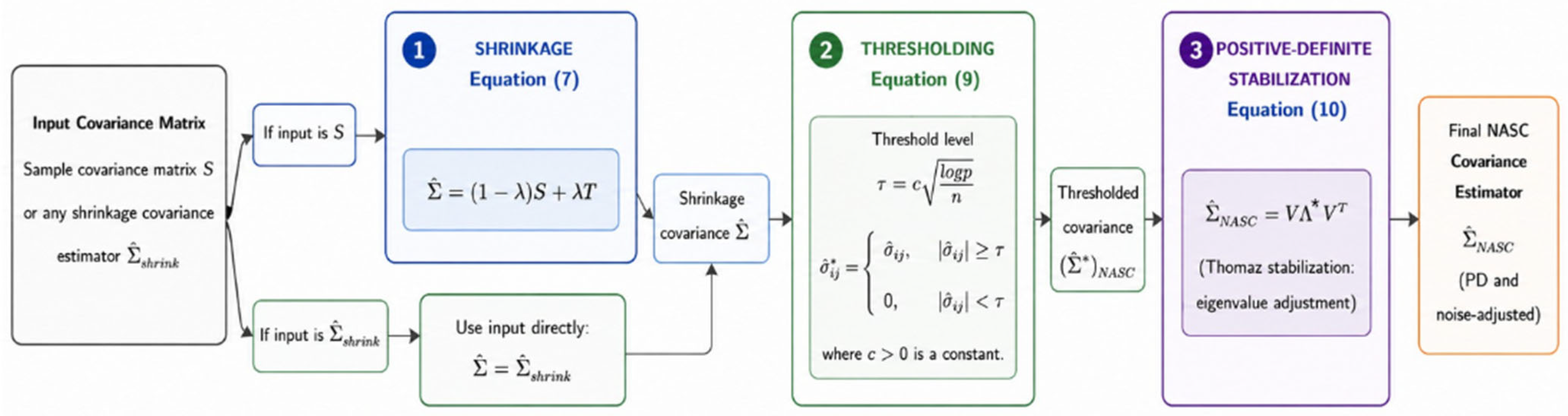
The NASC transformation is implemented through a three-stage process. In the first stage, a stabilized covariance estimator is obtained by shrinking the sample covariance matrix toward a structured target matrix using the shrinkage formulation given in Equation (7). In the second stage, the thresholding operator defined in Equation (8) is applied to the shrinkage estimator in order to suppress small covariance entries that are likely to arise from sampling noise. Finally, since entrywise thresholding may destroy the positive definiteness of the covariance matrix, a stabilization algorithm is applied to the resulting matrix to guarantee positive definiteness and improve numerical stability.

Formally, after the shrinkage and thresholding stages, the intermediate NASC estimator can be expressed compactly as

$${\widehat{{\mathsf{\Sigma }}^{*}}}_{NASC}=T_{\tau }\left({\widehat{\mathsf{\Sigma }}}_{shrink}\right)$$

(9)

where ${\widehat{\mathsf{\Sigma }}}_{shrink}$ denotes a generic shrinkage-based covariance estimator and $T_{\tau }\left(.\right)$ represents the thresholding operator applied with threshold level $\tau =c\sqrt{{\displaystyle \frac{logp}{n}}}$.

Structural Validity: Positive Definiteness

To ensure structural validity of the proposed estimator, we apply the stabilization algorithm proposed by Thomaz et al. (2004) to the NASC covariance estimator [32]. The basic idea of the Thomaz stabilization procedure is to adjust the eigenvalues of the estimated covariance matrix in order to guarantee that all eigenvalues remain strictly positive while preserving the overall covariance structure as much as possible.

The eigenvalue stabilization algorithm defined by Thomaz [32]:

• Step-1: Calculate the eigenvalues ${\lambda }_j$ and their eigenvectors $v_j$ of ${\widehat{{\mathsf{\Sigma }}^{\ast }}}_{NASC}$, where $j=1,2,\dots ,p$ and $p$ is the number of variables of the data.
• Step-2: Calculate the arithmetic mean of eigenvalues by using: $\overline{\lambda }={\displaystyle \frac{1}{p}}{\displaystyle {\sum }_{j=1}^p}{\lambda }_j$
• Step-3: Produce the following matrix of eigenvalues based on largest dispersion values:

  $${\mathsf{\Lambda }}^{\ast }=\left[\begin{array}{ccc}\max \left({\lambda }_1,\overline{\lambda }\right) 0& \dots & 0\\ ⋮& \ddots & ⋮\\ 0 0& \dots & \mathrm{m}\mathrm{a}\mathrm{x}({\lambda }_p,\overline{\lambda })\end{array}\right]$$
• Step-4: The new stabilized covariance matrix is given by:

  $${\widehat{\mathsf{\Sigma }}}_{NASC}=V{\mathsf{\Lambda }}^{\ast }{V}^T$$

  (10)

  where $V$ is matrix of eigenvectors $v_j$ of ${\widehat{{\mathsf{\Sigma }}^{\ast }}}_{NASC}$. As is seen, the algorithm stabilizes eigenvalues by expanding only the smaller and consequently less reliable eigenvalues of the covariance matrix and by keeping its larger eigenvalues unchanged. Since the adjusted eigenvalues are strictly positive, the resulting covariance estimator remains positive definite by construction.

Then, one can obtain NASC by following three stage process:

Stage-1: Compute the shrinkage covariance estimator ${\widehat{\mathsf{\Sigma }}}_{shrink}$ using the shrinkage formulation given in Equation (7).

Stage-2: Apply the thresholding operator defined in Equation (9) to the shrinkage estimator to remove noise-level correlations and compute ${\widehat{{\mathsf{\Sigma }}^{\ast }}}_{NASC}$.

Stage-3: Apply the Thomaz stabilization algorithm to the matrix ${\widehat{{\mathsf{\Sigma }}^{\ast }}}_{NASC}$ in order to guarantee positive definiteness.

The resulting matrix ${\widehat{\mathsf{\Sigma }}}_{NASC}$ in Equation (10) represents the final NASC-enhanced covariance estimate obtained from the selected shrinkage estimator.

Although the thresholding stage promotes sparsity by removing small covariance entries, the subsequent Thomaz stabilization step does not generally preserve the exact sparsity pattern. The primary role of thresholding within NASC is to suppress noise-level covariance entries before stabilization is applied. Consequently, the final NASC estimator should be interpreted as a noise-adjusted and positive-definite covariance estimator rather than a strictly sparse covariance estimator.

It is important to note that the NASC framework is not restricted to a single shrinkage formulation. Any shrinkage-based covariance estimator (e.g., Ledoit–Wolf, OAS, or other structured shrinkage estimators presented in Table 1) can be incorporated within this framework by replacing ${\widehat{\mathsf{\Sigma }}}_{shrink}$ in Equation (9). The overall workflow of the proposed NASC framework is illustrated in Figure 1.

Interpretation of the NASC framework via Error Decomposition

Let ${\widehat{\mathsf{\Sigma }}}_{shrink}$ denote the initial shrinkage estimator, $T_{\tau }\left({\widehat{\mathsf{\Sigma }}}_{shrink}\right)$ the thresholded covariance estimator, and ${\widehat{\mathsf{\Sigma }}}_{NASC}$ the final stabilized NASC estimator. The effect of NASC framework on the overall estimation error can be expressed by introducing the intermediate thresholded and shrinkage estimators as follows:

$${\widehat{\mathsf{\Sigma }}}_{NASC}-\mathsf{\Sigma }={\widehat{\mathsf{\Sigma }}}_{NASC}-T_{\tau }\left({\widehat{\mathsf{\Sigma }}}_{shrink}\right)+T_{\tau }\left({\widehat{\mathsf{\Sigma }}}_{shrink}\right)-{\widehat{\mathsf{\Sigma }}}_{shrink}+{\widehat{\mathsf{\Sigma }}}_{shrink}-\mathsf{\Sigma }$$

(11)

Taking Frobenius norms on both sides and applying the triangle inequality yields

$${‖{\widehat{\mathsf{\Sigma }}}_{NASC}-\mathsf{\Sigma }‖}_F\le {‖{\widehat{\mathsf{\Sigma }}}_{shrink}-\mathsf{\Sigma }‖}_F+{‖T_{\tau }\left({\widehat{\mathsf{\Sigma }}}_{shrink}\right)-{\widehat{\mathsf{\Sigma }}}_{shrink}‖}_F+{‖{\widehat{\mathsf{\Sigma }}}_{NASC}-T_{\tau }\left({\widehat{\mathsf{\Sigma }}}_{shrink}\right)‖}_F$$

(12)

This decomposition provides an intuitive interpretation of the NASC framework. The first term, represents the estimation error inherited from the underlying shrinkage estimator. The second term, quantifies the perturbation introduced by the thresholding step, which aims to suppress noise-induced small covariance entries and promote sparsity. The third term, captures the additional modification induced by the stabilization stage that restores positive definiteness of the covariance estimator.

Consequently, the total estimation error of the NASC framework may be viewed as the combined effect of three components: the baseline shrinkage estimation error, the thresholding perturbation, and the stabilization perturbation. Although this decomposition does not constitute a formal risk bound or asymptotic consistency result, it provides useful theoretical insight into the role of each stage within the NASC framework and clarifies how the proposed procedure modifies the original shrinkage estimator.

3. Numerical Examples

To investigate the behavior of the proposed NASC framework and evaluate its finite-sample performance, two sensitivity analyses and a Monte Carlo simulation study were conducted. The sensitivity analyses were designed to examine the effects of the shrinkage parameter $\lambda$ and the thresholding constant $c$ and to identify suitable parameter settings for the subsequent simulation study. The Monte Carlo experiment was then used to evaluate the estimation performance of the baseline NASC framework, the shrinkage estimators presented in Table 1, and their NASC-enhanced counterparts under different covariance structures and dimensionality regimes.

3.1. Simulation Settings

Population Covariance Structures: We use the following models for $\mathsf{\Sigma }$.

• Banded Sparse Covariance Structure:

  $${\mathsf{\Sigma }}_{ij}=\left\{\begin{array}{c}1,i=j\\ 0.3,\left|i-j\right|=1\\ 0.15,\left|i-j\right|=2\\ 0,\left|i-j\right|>2\end{array}\right. for 1\le i,j\le p$$
• Block-diagonal covariance structure: The covariance matrix consists of blocks of size $b={\displaystyle \frac{p}{10}}$, where within-block correlations are set to $0.5$ and between-block correlations are zero. If $p$ is not divisible by 10, the last block is taken in the remaining size. Let $k$ denote the number of blocks. Then ${{(\mathsf{\Sigma }}_k)}_{ij}=\left\{\begin{array}{c}1,i=j\\ 0.5,i\ne j\end{array}\right.$ $for 1\le i,j\le p$, and the overall covariance matrix is given by $\mathsf{\Sigma }=blockdiag\left({\mathsf{\Sigma }}_1,\dots ,{\mathsf{\Sigma }}_k\right)$.
• Autoregressive AR(1) covariance structure: ${\mathsf{\Sigma }}_{ij}={\rho }^{\left|i-j\right|} for 1\le i,j\le p$ and set $\rho =0.6$

Data Generation: $X_1,X_2,\dots ,X_n\in {\mathbb{R}}^p$ denote independent observations drawn from a multivariate normal distribution:

$$X_i~N_p\left(0,\mathsf{\Sigma }\right),i=1,\dots ,n$$

where Σ is the population covariance matrix defined above.

Sample Size and Dimension: The sample sizes considered are $nϵ\left\{30,50,100\right\}$. For each sample size, the dimensionality p is chosen such that the ratio ${\displaystyle \frac{n}{p}}$ takes the values: ${\displaystyle \frac{n}{p}}ϵ\left\{1,0.5,0.1,0.05\right\}$. This setup includes moderate as well as severe high-dimensional regimes, particularly cases where $n<<p.$

Performance Evaluation: The performance of the estimators was evaluated using the Frobenius loss defined in Equation (3), which measures the overall discrepancy between the estimated and true covariance matrices. For each combination of covariance model, sample size, and dimension, the simulation scenario was repeated over 1000 independent Monte Carlo replications, and the average loss across replications was used as the primary performance metric.

All simulation studies and covariance estimation procedures were conducted in MATLAB R2023a (MathWorks, Natick, MA, USA) on a 64-bit Windows-based system equipped with an Intel^® Core™ i7-13620H (13th Generation, 2.40 GHz) processor and 32 GB RAM. The total execution time of the simulation framework was approximately 21,194 s (about 5.88 h). The complete MATLAB implementation used in this study is provided in the Supplementary Materials.

3.2. Sensitivity Analysis

To investigate the sensitivity of the proposed NASC framework to its tuning parameters, two complementary sensitivity analyses were conducted. The first analysis focuses on the baseline NASC estimator obtained by applying the shrinkage operation defined in Equation (7), followed by the thresholding rule given in Equation (8) and the subsequent positive-definite stabilization step. Different combinations of the shrinkage weight $\lambda$ and thresholding constant $c$ were examined to evaluate the extent to which the baseline NASC formulation improves the estimation performance of the sample covariance matrix across different covariance structures and dimensionality regimes.

The second analysis focuses on the NASC-enhanced shrinkage estimators. In this case, each shrinkage estimator (EB, SRE, SDE, CSE, OAS, and LW) retained its original estimator-specific shrinkage intensity, while only the thresholding parameter c was varied. This analysis was designed to assess the sensitivity of the NASC enhancement procedure independently of the underlying shrinkage estimator.

For each parameter configuration, the squared Frobenius losses of the baseline and NASC-adjusted estimators were compared across all simulation scenarios. In the first sensitivity analysis, the baseline estimator refers to the sample covariance matrix (S), whereas in the second sensitivity analysis it refers to the corresponding shrinkage estimator (EB, SRE, SDE, CSE, OAS, or LW) prior to the NASC adjustment. An improvement was recorded whenever

$$Loss\left(NASC\right)<Loss\left(Baseline\right)$$

where $Loss$ denotes the squared Frobenius loss. The number of scenarios satisfying this condition was recorded as the number of improved cases. The improvement frequency was then calculated as

$$ImprovementFrequency\left(IF\%\right)={\displaystyle \frac{NumberofImprovedScenarios}{TotalNumberofScenarios}}\times 100$$

The results are reported both overall and separately for sparse, block-diagonal, and AR(1) covariance structures. The results of the two sensitivity analyses are presented in

Table 2. (a). Sensitivity analysis of the baseline NASC framework across different $\lambda$ and c configurations. (b). Sensitivity of NASC-enhanced shrinkage estimators to the thresholding constant $c.$

(a)
λ	c	Overall	Sparse	Block-Diagonal	AR(1)
0.25	0.5	36/36 (100.0%)	12/12 (100.0%)	12/12 (100.0%)	12/12 (100.0%)
0.25	1.0	36/36 (100.0%)	12/12 (100.0%)	12/12 (100.0%)	12/12 (100.0%)
0.25	1.5	32/36 (88.9%)	12/12 (100.0%)	8/12 (66.7%)	12/12 (100.0%)
0.25	2.0	29/36 (80.6%)	12/12 (100.0%)	5/12 (41.7%)	12/12 (100.0%)
0.50	0.5	36/36 (100.0%)	12/12 (100.0%)	12/12 (100.0%)	12/12 (100.0%)
0.50	1.0	30/36 (83.3%)	12/12 (100.0%)	6/12 (50.0%)	12/12 (100.0%)
0.50	1.5	29/36 (80.6%)	12/12 (100.0%)	5/12 (41.7%)	12/12 (100.0%)
0.50	2.0	27/36 (75.0%)	12/12 (100.0%)	5/12 (41.7%)	10/12 (83.3%)
0.75	0.5	30/36 (83.3%)	12/12 (100.0%)	6/12 (50.0%)	12/12 (100.0%)
0.75	1.0	27/36 (75.0%)	12/12 (100.0%)	5/12 (41.7%)	10/12 (83.3%)
0.75	1.5	27/36 (75.0%)	12/12 (100.0%)	5/12 (41.7%)	10/12 (83.3%)
0.75	2.0	27/36 (75.0%)	12/12 (100.0%)	5/12 (41.7%)	10/12 (83.3%)
1.00	0.5	27/36 (75.0%)	12/12 (100.0%)	5/12 (41.7%)	10/12 (83.3%)
1.00	1.0	27/36 (75.0%)	12/12 (100.0%)	5/12 (41.7%)	10/12 (83.3%)
1.00	1.5	27/36 (75.0%)	12/12 (100.0%)	5/12 (41.7%)	10/12 (83.3%)
1.00	2.0	27/36 (75.0%)	12/12 (100.0%)	5/12 (41.7%)	10/12 (83.3%)
(b)
$c$		Overall (%)	Sparse (%)	Block-Diagonal (%)	AR(1) (%)
0.5		127/216 (58.8%)	45/72 (62.5%)	49/72 (68.1%)	33/72 (45.8%)
1.0		139/216 (64.4%)	56/72 (77.8%)	42/72 (58.3%)	41/72 (56.9%)
1.5		127/216 (58.8%)	56/72 (77.8%)	30/72 (41.7%)	41/72 (56.9%)
2.0		120/216 (55.6%)	56/72 (77.8%)	23/72 (31.9%)	41/72 (56.9%)

.

The sensitivity analysis presented in Table 2 reveals several noteworthy patterns regarding the behavior of the baseline NASC estimator. First, NASC exhibited remarkable robustness under sparse covariance structures. Across all investigated combinations of the shrinkage parameter $\lambda$ and the thresholding constant $c$, NASC achieved lower Frobenius loss than the sample covariance matrix in all 12 sparse scenarios, corresponding to a 100% improvement frequency. This finding suggests that the sequential shrinkage–thresholding–stabilization strategy is particularly effective when the underlying covariance structure contains a large number of negligible covariance entries.

In contrast, the block-diagonal covariance structure was found to be the most sensitive to parameter selection. While NASC improved upon the sample covariance matrix in all block-diagonal scenarios when $\lambda =0.25$ and $c\le 1.0$, the improvement frequency gradually decreased as the regularization became more aggressive, reaching 66.7%, 50.0%, and ultimately 41.7% for larger $\lambda$ and $c$ values. This pattern suggests that excessive shrinkage and thresholding may remove covariance information associated with the true block structure, thereby reducing the relative advantage of the NASC transformation.

The AR(1) covariance structure exhibited intermediate behavior. For smaller $\lambda$ values, NASC improved the estimation performance in all considered scenarios. As $\lambda$ increased, the improvement frequency decreased slightly to 83.3%, indicating that dense dependence structures are somewhat more sensitive to regularization than sparse structures, although considerably less sensitive than block-diagonal covariance matrices.

Overall, the highest improvement frequency was obtained for the parameter combinations $(\lambda ,c)=(0.25,0.5)$ and $(0.25,1.0)$, where NASC outperformed the sample covariance matrix in all 36 simulation scenarios.

Table 2 summarizes the sensitivity of the NASC-enhanced shrinkage estimators to the thresholding constant $c$. The highest overall improvement frequency was obtained at $c=1.0$ (64.4%), indicating that moderate thresholding provides the most favorable balance between noise suppression and covariance structure preservation. The strongest improvements were observed under sparse covariance structures, where improvement frequencies reached 77.8%. In contrast, performance decreased progressively for block-diagonal structures as c increased, suggesting that aggressive thresholding may remove meaningful covariance information within dense blocks. AR(1) structures exhibited intermediate behavior, with improvement frequencies stabilizing at 56.9% once $c\ge 1$. Overall, the results support the use of $(c=1)$. Since the parameter combination achieved the highest overall improvement frequency in the baseline sensitivity analysis while also demonstrating consistent performance across all covariance structures, this configuration was adopted in the subsequent Monte Carlo simulation study.

The simulation study was designed to evaluate the NASC framework from several complementary perspectives. First, the ability of NASC to improve existing shrinkage estimators was examined by comparing each shrinkage estimator with its NASC-enhanced counterpart. Second, the behavior of the framework was investigated under sparse, block-diagonal, and AR(1) covariance structures. Third, the effect of dimensionality was assessed across different p/n ratios. Finally, the baseline NASC estimator constructed using the parameter configuration selected from the sensitivity analyses ($(\lambda ,c)=(0.25,1)$) was directly compared with the conventional shrinkage estimators in order to evaluate its standalone performance relative to existing shrinkage approaches.

3.3. Monte-Carlo Simulation

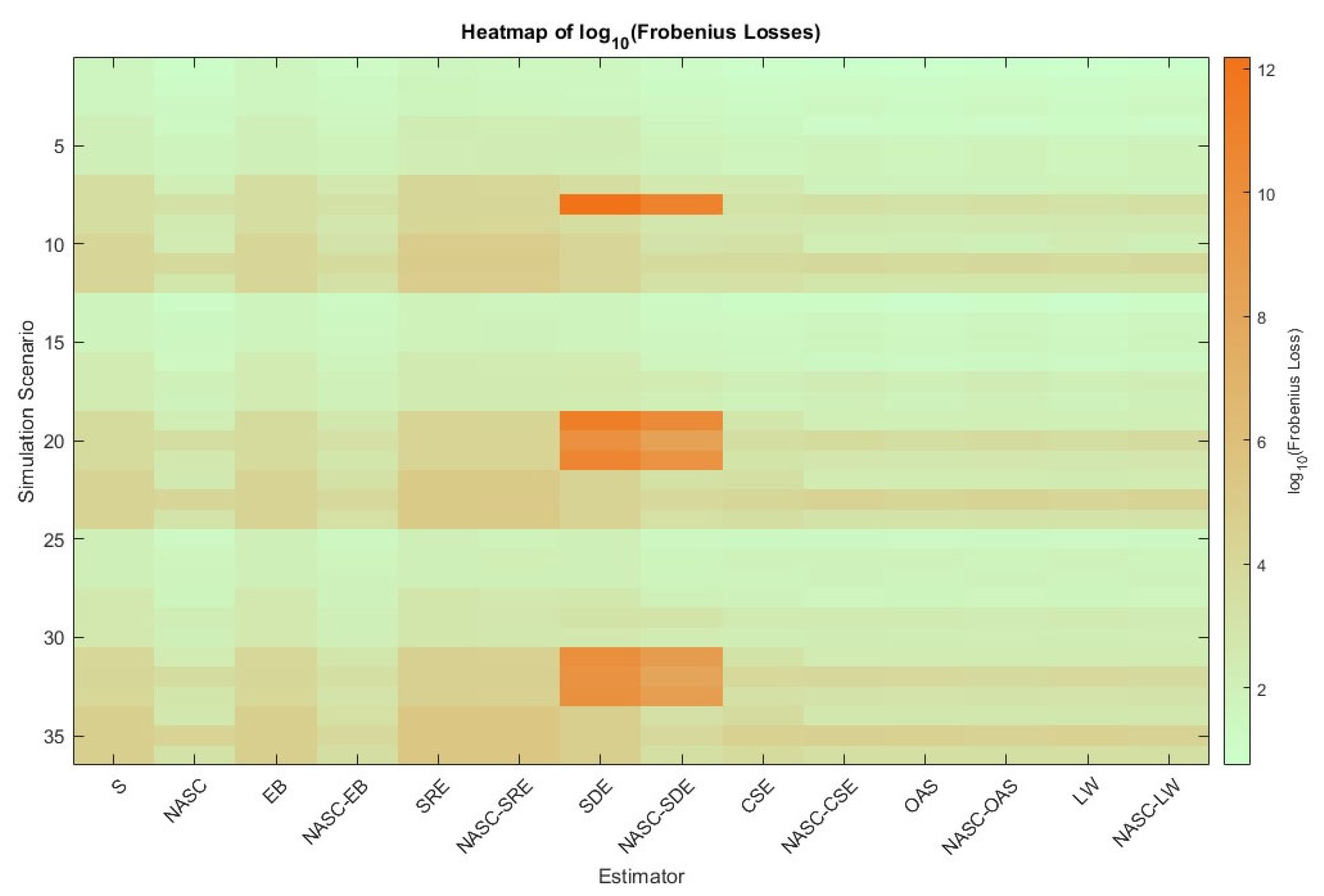
The complete simulation results, including the Frobenius loss values obtained for all covariance structures, dimensionality settings, and competing estimators, are provided in Supplementary Table S1. To facilitate interpretation of these results, Figure 2 presents a heatmap of the log-transformed loss values reported in Supplementary Table S1, providing an overall visual comparison of estimator performance across all simulation scenarios. In addition, the main findings are summarized in

Table 3. Frequency with which the NASC transformation improves the corresponding shrinkage estimator.

Baseline Shrinkage Estimator	Improved Cases	Total Scenarios	Improvement Rate (%)
${\widehat{\mathsf{\Sigma }}}_{EB}$	36	36	100.0
${\widehat{\mathsf{\Sigma }}}_{SRE}$	30	36	83.3
${\widehat{\mathsf{\Sigma }}}_{SDE}$	36	36	100.0
${\widehat{\mathsf{\Sigma }}}_{CSE}$	20	36	55.6
${\widehat{\mathsf{\Sigma }}}_{OAS}$	7	36	19.4
${\widehat{\mathsf{\Sigma }}}_{LW}$	10	36	27.8
Overall	139	216	64.4

,

Table 4. Structure-specific effectiveness of the NASC framework.

Covariance Structure	Improved Cases	Total Comparisons	Improvement Rate (%)
Sparse	56	72	77.8
Block-Diagonal	42	72	58.3
AR(1)	41	72	56.9
Overall	139	216	64.4

and

Table 5. Effect of the Dimensionality Ratio (p/n) on the Improvement Frequency of the NASC Framework.

p/n Ratio	Improved Cases	Total Comparisons	Improvement Rate (%)
1	31	54	57.4
2	33	54	61.1
10	36	54	66.7
20	39	54	72.2
Overall	139	216	64.4

using improvement frequencies and comparative performance measures. These summary tables highlight different aspects of the NASC framework, including its effectiveness across shrinkage estimators, covariance structures, dimensionality regimes, and its performance relative to existing shrinkage estimators.

Table 3 summarizes the frequency with which the NASC transformation improved the corresponding shrinkage estimator across all 36 simulation scenarios. The highest improvement rates were observed for the Empirical Bayes (EB) and Stipulated Diagonal Estimator (SDE), where the NASC-adjusted versions achieved lower Frobenius losses in all scenarios (100%). Some SDE scenarios exhibited extremely large Frobenius losses in $n\ll p$ settings, likely reflecting numerical instability associated with the Moore–Penrose pseudo-inverse. Therefore, the high improvement frequency observed for NASC-SDE is expected and should be interpreted mainly as a consequence of stabilizing a numerically unstable baseline estimator. NASC improved the performance of the Stipulated Ridge Estimator (SRE) in 83.3% of the cases. More moderate improvement frequencies were obtained for the Convex Sum Estimator (CSE), with improvements observed in 55.6% of the scenarios. In contrast, the Oracle Approximating Shrinkage (OAS) and Ledoit–Wolf (LW) estimators were improved less frequently, with improvement rates of 19.4% and 27.8%, respectively. Overall, the NASC transformation reduced the estimation loss in 139 of the 216 estimator–scenario comparisons, corresponding to an overall improvement rate of 64.4%. These results indicate that the effectiveness of the NASC transformation depends on the underlying shrinkage estimator. The largest gains were obtained for estimators that do not explicitly control entrywise estimation noise, whereas the benefits were naturally smaller for highly optimized shrinkage estimators such as OAS and LW.

Table 4 presents the effectiveness of the NASC transformation across different population covariance structures. The results are obtained by aggregating the improvement frequencies of all NASC-adjusted shrinkage estimators within each covariance structure.

As shown in Table 4, the highest improvement frequency was observed under sparse covariance structures, where NASC achieved lower Frobenius losses in 56 of the 72 shrinkage-estimator comparisons, corresponding to an improvement rate of 77.8%. In contrast, the improvement frequencies were lower for the block-diagonal and AR(1) covariance structures, with rates of 58.3% and 56.9%, respectively. Overall, NASC improved the corresponding shrinkage estimator in 139 of the 216 comparisons (64.4%). These findings indicate that while NASC provides benefits across all considered covariance models, its strongest gains are observed under sparse covariance settings.

Table 5 presents the effectiveness of the NASC transformation across different dimensionality settings. Similar to Table 2, the reported results were obtained by aggregating the improvement frequencies of all NASC-adjusted shrinkage estimators within each p/n ratio.

As shown in Table 5, the improvement frequency increased progressively as the dimensionality became larger relative to the sample size. When $n=p(p/n=1)$, NASC improved the corresponding shrinkage estimator in 31 of the 54 comparisons (57.4%). This rate increased to 61.1% and 66.7% for $p/n=2$ and $p/n=10$, respectively, and reached its highest value of 72.2% when $p/n=20$. These results indicate that the benefit of the NASC framework becomes more pronounced as the dimensionality increases. The observed trend suggests that the proposed correction is particularly effective in high-dimensional settings, where estimation noise and covariance matrix instability become increasingly severe.

3.4. Real Data Example

In this study, the SRBCT dataset [33] was used to evaluate the numerical stability of the proposed NASC framework under high-dimensional conditions, whereas the colon cancer dataset [34] was used to assess the LOOCV-LDA classification performance of the most competitive covariance estimators.

The Small Round Blue Cell Tumor (SRBCT) dataset is a widely used benchmark dataset in high-dimensional classification and covariance estimation studies. The dataset contains gene expression measurements obtained from cDNA microarray experiments and consists of 63 training samples belonging to four tumor classes: Ewing’s sarcoma (EWS, $n$ = 23), Burkitt lymphoma (BL, $n$ = 8), Neuroblastoma (NB, $n$ = 12), and Rhabdomyosarcoma (RMS, $n$ = 20). Each sample includes expression levels for 2308 genes, resulting in a typical high-dimensional setting where the number of variables substantially exceeds the number of observations ($n\ll p$) [33].

The colon cancer dataset is a well-known high-dimensional gene expression dataset originally introduced by Alon et al. for studying tumor classification problems. The dataset consists of gene expression measurements obtained from colon tissue samples, including both tumor and normal tissues. After preprocessing, the dataset contains expression levels for 2000 genes measured across 62 samples, of which 40 correspond to tumor tissues and 22 correspond to normal tissues [34].

To evaluate the practical behavior of the proposed covariance estimation framework, the SRBCT benchmark dataset was analyzed from two complementary perspectives. First, all covariance estimators were compared in terms of their numerical stability properties, including condition number (CN) and positive definiteness characteristics assessed through the minimum eigenvalue of the estimated covariance matrices. The condition number of an estimated covariance matrix $\widehat{\mathsf{\Sigma }}$ was defined as

$$\kappa \left(\widehat{\mathsf{\Sigma }}\right)={\displaystyle \frac{{\lambda }_{max}\left(\widehat{\mathsf{\Sigma }}\right)}{{\lambda }_{min}\left(\widehat{\mathsf{\Sigma }}\right)}}$$

where ${\lambda }_{max}\left(\widehat{\mathsf{\Sigma }}\right)$ and ${\lambda }_{min}\left(\widehat{\mathsf{\Sigma }}\right)$ denote the largest and smallest eigenvalues of $\widehat{\mathsf{\Sigma }}$, respectively. Smaller condition number values indicate better numerical conditioning and greater stability of the covariance estimator. An estimated covariance matrix satisfying this condition is strictly positive definite, whereas values close to zero indicate near-singularity and numerical instability. Negative minimum eigenvalues imply that the covariance estimator is not positive definite.

As an additional evaluation, the classification performances of the baseline NASC estimator, OAS, and LW estimators, which were identified as the most competitive estimators in the simulation study, were examined within a Linear Discriminant Analysis (LDA) framework using the leave-one-out cross-validation (LOOCV) procedure on the colon cancer dataset. The results are presented

Table 6. Numerical stability and positive definiteness properties of covariance estimators on the SRBCT dataset.

Covariance Estimator	Minimum Eigvalue	$\mathit{\kappa }\left(\widehat{\mathsf{\Sigma }}\right)$
$S$	−5.93 × 10−14	7.76 × 1021
${\widehat{\mathsf{\Sigma }}}_{NASC}$	0.70	45.53
${\widehat{\mathsf{\Sigma }}}_{EB}$	0.03	3408.48
${\widehat{\mathsf{\Sigma }}}_{NASC\_EB}$	0.34	252.76
${\widehat{\mathsf{\Sigma }}}_{SRE}$	44.98	3.95
${\widehat{\mathsf{\Sigma }}}_{NASC\_SRE}$	45.39	2.90
${\widehat{\mathsf{\Sigma }}}_{SDE}$	−5.93 × 10−14	7.76 × 1021
${\widehat{\mathsf{\Sigma }}}_{NASC\_SDE}$	0.32	270.33
${\widehat{\mathsf{\Sigma }}}_{CSE}$	0.37	218.69
${\widehat{\mathsf{\Sigma }}}_{NASC\_CSE}$	0.63	68.85
${\widehat{\mathsf{\Sigma }}}_{OAS}$	0.30	310.40
${\widehat{\mathsf{\Sigma }}}_{NASC\_OAS}$	0.49	103.64
${\widehat{\mathsf{\Sigma }}}_{LW}$	1	1
${\widehat{\mathsf{\Sigma }}}_{NASC\_LW}$	1	1

and

Table 7. LOOCV-LDA Classification Performance of the Most Competitive Covariance Estimators on the Colon Cancer Dataset.

Covariance Estimator	LOOCV Accuracy	TN	FP	FN	TP	Sensitivity	Specificity	Precision	F1-Score
${\widehat{\mathsf{\Sigma }}}_{NASC}$	0.56	11	11	16	24	0.60	0.50	0.69	0.64
${\widehat{\mathsf{\Sigma }}}_{OAS}$	0.53	2	20	9	31	0.78	0.09	0.61	0.68
${\widehat{\mathsf{\Sigma }}}_{LW}$	0.60	10	12	13	27	0.68	0.45	0.69	0.68

.

Table 6 summarizes the numerical stability and positive definiteness properties of the covariance estimators on the SRBCT dataset. The sample covariance matrix (S) and the SDE estimator exhibited near-singular behavior, with minimum eigenvalues numerically close to zero and extremely large condition numbers (7.76 × 10²¹). In contrast, the NASC-adjusted estimators substantially improved both positive definiteness and numerical conditioning. The most notable improvement was observed for the SDE estimator, whose condition number decreased from 7.76 × 10²¹ to 270.33 after applying NASC. Similar improvements were also observed for the EB, CSE, and OAS estimators. Overall, the results confirm that the NASC framework successfully achieves its intended objective of improving positive definiteness and numerical conditioning in high-dimensional covariance estimation.

Table 7 presents the LOOCV-LDA classification results of the most competitive covariance estimators on the colon cancer dataset. Among the considered estimators, the LW estimator achieved the highest classification accuracy (0.60), followed by NASC (0.56) and OAS (0.53). Although the observed accuracies do not exceed the majority-class baseline of the dataset, the primary purpose of this experiment was not to maximize predictive performance. Rather, the objective was to evaluate the behavior of different covariance estimators when directly incorporated into an LDA classifier without any prior feature selection, dimensionality reduction, or variable screening. When considered together with the numerical stability results reported in Table 6, these findings illustrate the practical applicability of the NASC framework in high-dimensional settings.

4. Conclusions and Discussion

The primary motivation of this study was the observation that shrinkage and thresholding methods are typically applied as separate covariance estimation strategies and subsequently used as final covariance estimators. Although both approaches have been shown to improve estimation performance in high-dimensional settings, neither approach alone may be sufficient to simultaneously address estimation noise, structural preservation, and numerical stability. Motivated by this limitation, we proposed the NASC framework as a sequential procedure that combines shrinkage, thresholding, and positive-definite stabilization within a unified covariance estimation strategy. An important feature of the proposed framework is that it is not tied to a specific shrinkage estimator. While the baseline NASC formulation can be directly applied to the sample covariance matrix, the same procedure can also be used as a post-processing enhancement step for existing shrinkage estimators. Therefore, the main objective of this study was not to introduce another shrinkage estimator, but rather to investigate whether a systematic shrinkage–thresholding–stabilization procedure can provide additional improvements over existing covariance estimation approaches.

To address this question, extensive sensitivity analyses and Monte Carlo simulations were conducted. The sensitivity analyses demonstrated that the baseline NASC estimator consistently improved upon the sample covariance matrix across all sparse covariance scenarios and achieved its most stable overall performance for the parameter configuration ($(\lambda ,c)=(0.25,1)$). Consequently, this configuration was adopted for the baseline NASC estimator in the subsequent simulation study, while the NASC-enhanced shrinkage estimators retained their original estimator-specific shrinkage intensities and used the thresholding constant $(c=1)$.

The Monte Carlo results provided strong evidence that the effectiveness of the NASC framework depends on both the underlying shrinkage estimator and the covariance structure. Overall, NASC reduced the Frobenius loss in 139 of the 216 shrinkage-estimator comparisons, corresponding to an improvement frequency of 64.4%. The largest gains were observed for the EB, SDE, and SRE estimators, whereas more modest improvements were obtained for highly optimized shrinkage estimators such as OAS and LW. When examined across covariance structures, the strongest improvements were observed under sparse covariance models, where the improvement frequency reached 77.8%. Furthermore, the improvement frequency increased steadily as the dimensionality increased, reaching 72.2% in the most challenging high-dimensional setting ((p/n = 20)). These findings suggest that the proposed framework becomes increasingly beneficial as estimation noise and covariance matrix instability become more pronounced.

The real-data analyses demonstrate the practical numerical and predictive behavior of the proposed framework. On the SRBCT benchmark dataset, the NASC framework substantially improved numerical stability and positive definiteness properties compared with several conventional covariance estimators. In particular, the NASC-adjusted estimators achieved considerably smaller condition numbers and strictly positive minimum eigenvalues, whereas the sample covariance matrix and some shrinkage estimators exhibited near-singular behavior under severe high-dimensional conditions. These results demonstrate that the NASC framework not only improves covariance estimation accuracy in simulations but also enhances the practical numerical stability of covariance estimation in real high-dimensional datasets.

Similarly, the LOOCV-LDA classification analysis on the colon cancer dataset showed that the NASC estimator achieved competitive classification performance relative to OAS and LW without requiring any prior feature selection or dimensionality reduction. It should be emphasized that the primary objective of the real-data analyses was not to achieve the highest possible classification accuracy. Rather, the aim was to compare the ability of the covariance estimators to perform classification within a basic LDA framework under severe high-dimensional conditions, without applying any prior feature selection or dimensionality reduction procedure. Taken together, the simulation and real-data analyses suggest that the proposed NASC framework provides a practical emprically motivated extension to classical shrinkage covariance estimation methods for challenging high-dimensional applications.

Furthermore, the performance of the NASC framework is expected to depend on the selection of both the shrinkage structure and the thresholding parameter $c$. Although sensitivity analyses were conducted in the present study, these analyses were based on a limited set of representative parameter values and were primarily intended to assess the robustness of the framework rather than to identify globally optimal tuning parameters. In particular, incorporating a data-adaptive shrinkage mechanism together with a data-driven selection of the threshold constant may further improve the estimation and classification performance of the proposed framework. Future studies may therefore focus on developing adaptive parameter selection strategies for the NASC procedure, including cross-validation-based approaches, Stein-type risk minimization methods, and information-criterion-based tuning schemes. Such extensions may provide a fully data-adaptive implementation of NASC and further enhance its practical performance in high-dimensional settings. Another potential direction for future research is to investigate the individual contributions of the thresholding and stabilization stages through ablation-type analyses and to examine how sparsity patterns evolve before and after the positive-definite stabilization step. In addition, the performance of the NASC framework under heavy-tailed and non-Gaussian distributions may also be investigated in future studies in order to assess its robustness beyond the multivariate normal setting.