Generalized Lucky Numbers for H(r) Architectures

Abstract

A lucky coloring of a graph G is an edge coloring induced by a vertex labeling, where each edge is assigned a color equal to the sum of the labels of its incident vertices, such that adjacent edges receive distinct colors. The lucky number of G, denoted by $\eta \left(G\right)$, is the minimum integer k such that G admits a lucky coloring using labels from the set $\{1,2,3,\dots ,k\}$. In this paper, we investigate the lucky numbers for the $H\left(r\right)$ architectures, a sequence of r connected H-shaped structures. We establish the exact values for these graphs, proving that $\eta \left(H\right(r\left)\right)=6$ for even r and $\eta \left(H\right(r\left)\right)=7$ for odd $r\ge 3$.

1. Introduction

In 2014, Murugan and Chitra [1] introduced the basic concept of lucky coloring for simple graphs, originally known as lucky edge coloring. For a graph $G=\left(V\right(G),E(G\left)\right)$, where $V\left(G\right)$ is the vertex set and $E\left(G\right)$ is the edge set, a lucky edge coloring is induced by a vertex coloring. Given a vertex coloring function $f:V\left(G\right)\to T$ where $T=\{1,2,3,\dots \}$, the induced edge coloring $f^{*}:E\left(G\right)\to \{2,3,4,\dots \}$ is defined as $f^{*}\left(ab\right)=f\left(a\right)+f\left(b\right)$ for each edge $ab\in E\left(G\right)$. The edge coloring $f^{*}$ is called a lucky coloring if $f^{*}\left(e_1\right)\ne f^{*}\left(e_2\right)$ whenever $e_1$ and $e_2$ are adjacent edges. The least integer k such that there exists a lucky coloring of G using vertex labels from the set $\{1,2,3,\dots ,k\}$ is called the lucky number of G, denoted by $\eta \left(G\right)$. Numerous mathematicians have conducted studies on lucky colorings and lucky numbers, leading to several important results. In 2014, Murugan and Chitra [2] investigated the lucky numbers of path graphs $P_n$, cycle graphs $C_n$, and the coronas of $P_n$ and $C_n$, finding them to be $4,6,5$, and 6, respectively. Later, in 2015 [3], the same authors established that the lucky number of the H-graph is 6. In 2016, Sridevi and Ragavi [4] investigated lucky colorings for complete graphs $K_n$, complete bipartite graphs $K_{m,n}$, and dragon graphs $T_{m,n}$, determining their lucky numbers to be $2n-1$, $m+n$, and $\{5,6\}$, respectively. In the same year, Murugan and Chitra [5] found the lucky numbers for the triangular snake graph $T_n$ and the triangular prism graph to be 8 and $\{8,12\}$, respectively. In 2017 [6], Esakkiamma et al. determined the lucky numbers for the super subdivision of star graphs $SS\left(S_n\right)$ and wheel graphs $SS\left(W_n\right)$. Additionally, the lucky edge labeling of H-super subdivision of graphs was investigated in [7]. Furthermore, in 2018, Chitra and Murugan [1] presented the lucky numbers for various graphs, establishing that $\eta \left(K_{1,1,n}\right)=n+4$, $\eta \left(D_2\left(P_n\right)\right)=8$, $\eta \left(M\left(P_n\right)\right)=9$, $\eta \left(F_{sn}\right)=n+4$, and $\eta (P_n+S_m)=7$. Later, in 2019, Babu, Ramya, and Thirusangu [8] established that the lucky numbers of the splitting graph $S\left(G\right)$ and the alternate triangular snake graph $A\left(T_n\right)$ are $2n+1$ and 7, respectively. In the same year, Ramya and Shalini [9] investigated firecracker graphs $P_n\odot S_m$ and twig graphs $T_m$, finding their lucky numbers to be $m+3$ (for $m\le n$) or $m+4$ (for $m=n$), and 6, respectively. Subsequently, in 2021, Shalini et al. [10] studied the lucky colorings for various graph classes, including the theta graph $T_{\alpha }$, multiple copies of $T_{\alpha }$ and H, and duplications of the path union of $T_{\alpha }$, explicitly determining their exact lucky numbers. Most recently, in 2023, Ananthayasedthi et al. [11] provided necessary conditions for classifying lucky colorings of general graphs. They also demonstrated essential properties of lucky colorings and derived the lucky numbers for rooted tree graphs $T_{m,h}$ based on their height h, establishing the lucky numbers to be $2m+1$ for $h=3$, and $2m+2$ for $h\ge 4$. While the lucky numbers of various fundamental graphs have been extensively studied, there remains a gap in understanding more complex sequential architectures. The $H\left(r\right)$ architecture, which represents a sequence of r connected H-shaped structures, is of particular significance. Studying this class of graphs provides deeper insights into the behavior of edge colorings induced by vertex constraints within repetitive or modular frameworks, which can serve as theoretical models for sequential network topologies and chemical polymer chains. In this paper, we extend the concept of lucky colorings specifically to $H\left(r\right)$ architectures, determining their exact lucky numbers based on parity. Finally, Section 3 provides the discussion and directions for future research.

2. Preliminaries and Graph Architecture

In this section, we present the foundational definitions, notations, and structural properties utilized throughout this manuscript. To improve clarity and readability, the preliminary results are organized into logical subsections focusing on the coloring mechanisms, the structural definition of the sequential architecture, and its fundamental regularity properties.

2.1. Lucky Coloring and Labeling

We begin by formalizing the core concept of lucky coloring, which establishes how vertex labels induce distinct edge weights on adjacent edges.

Definition 1.

Let $G=(V,E)$ be a simple graph. A vertex-coloring function $f:V\left(G\right)\to \{1,2,3,...,k\}$ induces an edge coloring $f^{*}:E\left(G\right)\to \mathbb{N}$ defined by $f^{*}\left(uv\right)=f\left(u\right)+f\left(v\right)$ for each edge $uv\in E\left(G\right)$. The function f is called a lucky coloring if $f^{*}\left(e_1\right)\ne f^{*}\left(e_2\right)$ for any two adjacent edges $e_1,e_2\in E\left(G\right)$. The smallest integer k for which G admits a lucky coloring is called the lucky number of G, denoted by $\eta \left(G\right)$.

The following property, established by Ananthayasedthi et al., translates the edge-sum distinctness condition of a lucky coloring into an equivalent structural constraint on the neighborhoods of the vertices. This property serves as the primary mathematical tool for verifying valid colorings in our main results.

Proposition 1

(Anantayasethi et al. [11]). Let f be a vertex coloring of a graph G. The following statements are equivalent:

(i) 

     $f^{*}$ is a lucky coloring of G.

(ii) 

    $f\left(u_1\right)\ne f\left(u_2\right)$ for all $u_1,u_2\in N\left(v\right)$ with $u_1\ne u_2$ and for all $v\in V\left(G\right)$.

(iii) 

   $\left|N\right(v\left)\right|=\left|f\right(N\left(v\right)\left)\right|$ for all $v\in V\left(G\right)$.

2.2. The $H\left(r\right)$ Graph Architecture

To analyze sequential structures, we formally define the $H\left(r\right)$ graph architecture, which consists of r connected H-shaped units. To ensure global structural uniformity and prevent boundary discrepancies, we explicitly define the connection topology, including the continuous boundary wrap-around edges.

Definition 2.

Let $r\ge 2$ be a positive integer. The graph $H\left(r\right)$, representing a sequential H-architecture, is a simple graph structured over three horizontal tracks across $2r$ columns. The vertex set is given by

$$V\left(H\right(r\left)\right)=\left\{\right(i,j)\mid 1\le i\le 3and1\le j\le 2r\}.$$

The edge set is precisely defined as $E\left(H\left(r\right)\right)=E_1\cup E_2\cup E_3\cup E_4$, where

• $E_1=\{((i,j),(i,j+1))\mid i\in \{1,3\}and1\le j\le 2r-1\}$ (horizontal track edges);
• $E_2=\{((2,j),(2,j+1))\mid jisanoddnumberand1\le j\le 2r-1\}$ (central cross-track links);
• $E_3=\{((1,1),(1,2r)),((3,1),(3,2r))\}$ (boundary wrap-around connection edges);
• $E_4=\{((i,j),(i+1,j))\mid i\in \{1,2\}and1\le j\le 2r\}$ (vertical interior structural edges).

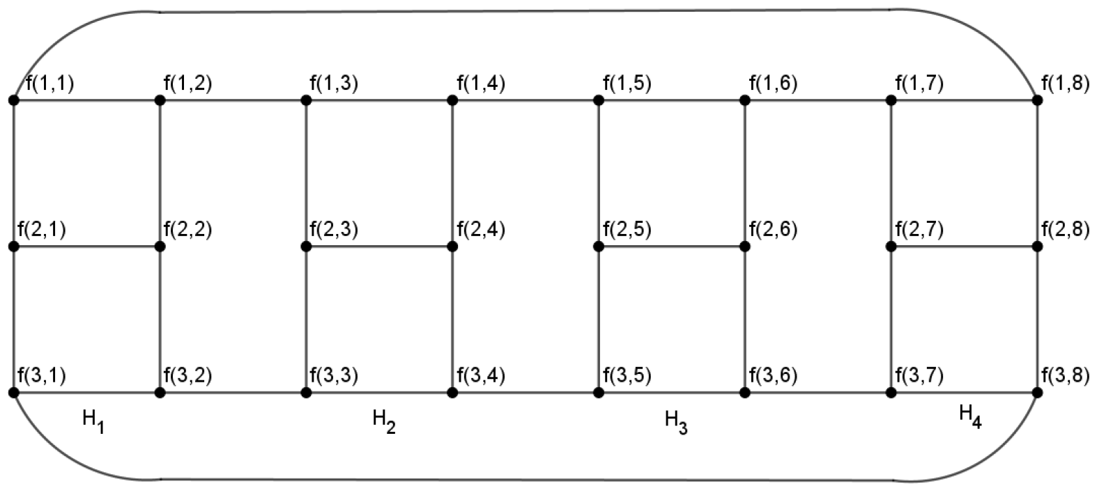
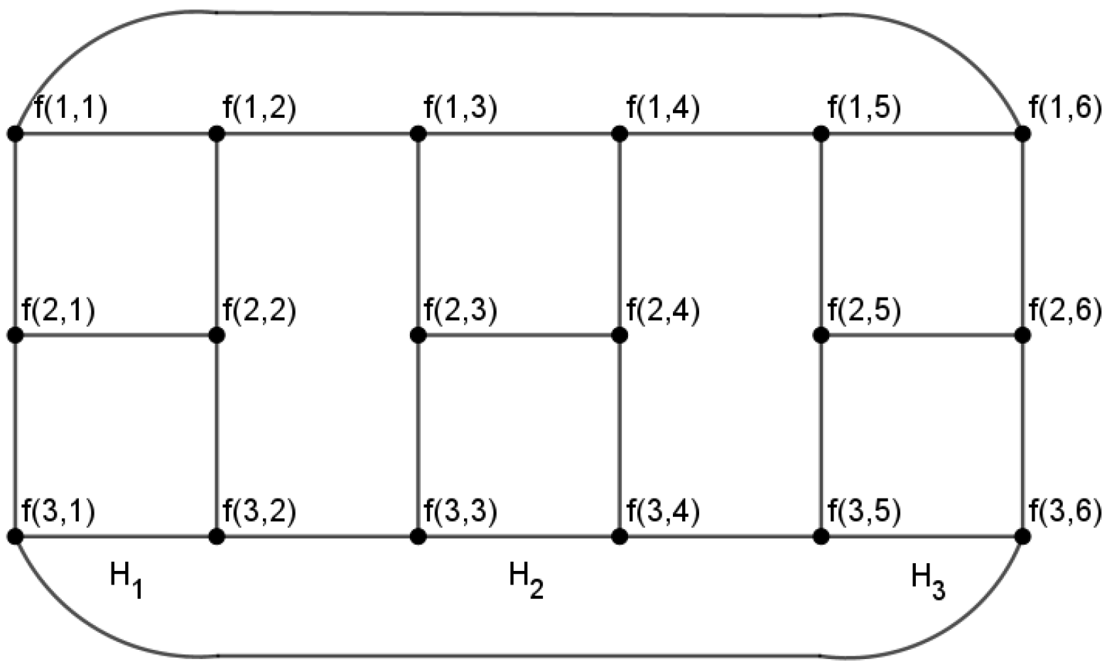
Geometrically, the graph $H\left(r\right)$ resembles r instances of the letter ’H’ arranged in a continuous, symmetric sequence. We denote the k-th ’H’ subgraph in this sequence as $H_k$, where $1\le k\le r$. Under this rigorous formulation, the precise neighborhood $N(i,j)$ for every vertex can be systematically identified, confirming that boundary columns $j=1$ and $j=2r$ seamlessly maintain structural continuity via $E_3$.

2.3. Structural Regularity

Before proceeding to the coloring proofs, we establish the fundamental degree properties of the $H\left(r\right)$ architecture derived from Definition 2.

Lemma 1.

The sequential graph architecture $H\left(r\right)$ is a 3-regular graph for any positive integer $r\ge 2$.

Proof. 

We verify the degree $d(i,j)$ for each vertex $(i,j)\in V\left(H\right(r\left)\right)$ by examining the defined edge sets:

1.

For the top track ($i=1$):

• If $1<j<2r$, the vertex $(1,j)$ is incident to two horizontal edges from $E_1$ (to $(1,j-1)$ and $(1,j+1)$) and one vertical edge from $E_4$ (to $(2,j)$). Thus, $d(1,j)=3$.
• If $j=1$, the vertex $(1,1)$ is incident to one horizontal edge from $E_1$ (to $(1,2)$), one vertical edge from $E_4$ (to $(2,1)$), and one boundary wrap-around edge from $E_3$ (to $(1,2r)$). Thus, $d(1,1)=3$.
• If $j=2r$, the vertex $(1,2r)$ is incident to one horizontal edge from $E_1$ (to $(1,2r-1)$), one vertical edge from $E_4$ (to $(2,2r)$), and one boundary wrap-around edge from $E_3$ (to $(1,1)$). Thus, $d(1,2r)=3$.

2.

For the bottom track ($i=3$): By symmetric logic applied to edge sets $E_1,E_3,$ and $E_4$, every vertex $(3,j)$ yields $d(3,j)=3$ for all $1\le j\le 2r$.

3.

For the central track ($i=2$): Every vertex $(2,j)$ is incident to exactly two vertical edges from $E_4$ (connected to $(1,j)$ and $(3,j)$). Additionally, from $E_2$:

• If j is odd, $(2,j)$ is connected horizontally to $(2,j+1)$.
• If j is even, $(2,j)$ is connected horizontally to $(2,j-1)$.

Therefore, every vertex on the central track is incident to exactly one horizontal edge and two vertical edges, giving $d(2,j)=3$ for all $1\le j\le 2r$.

Since $d(i,j)=3$ holds universally across all tracks and columns, $H\left(r\right)$ is strictly a 3-regular graph. In this section, we present the foundational definitions, notation, and existing theorems utilized throughout this manuscript. To maintain conciseness, standard graph-theoretic terminology—such as vertex sets, edge sets, and basic graph classes—follows standard mathematical conventions and is assumed to be familiar to the reader. □

3. Main Results

In this paper, we investigate the lucky coloring and determine the exact lucky number, $\eta \left(H\right(r\left)\right)$, for the $H\left(r\right)$ graph architecture. We analyze these graphs by classifying them into two distinct cases based on the parity of r. Our main results demonstrate that if r is a positive even integer, $\eta \left(H\right(r\left)\right)=6$, whereas if r is a positive odd integer, $\eta \left(H\right(r\left)\right)=7$. Detailed proofs for both cases are provided in the subsequent subsections.

Example 1.

An example of the $H\left(r\right)$ graph architecture when r is a positive even integer is illustrated in Figure 1.

Example 2.

An example of the $H\left(r\right)$ graph architecture when r is a positive odd integer is illustrated in Figure 2.

Lemma 2.

If $f^{*}$ is a k-lucky coloring of $H\left(r\right)$ and $k\in \{5,6\}$, then $f\left(u\right)\le 3$ for all $u\in V\left(H\right(r\left)\right)$.

Proof. 

We proceed by contradiction. Assume that $f^{*}$ is a k-lucky coloring of $H\left(r\right)$ for $k\in \{5,6\}$, but suppose there exists some vertex $u\in V\left(H\right(r\left)\right)$ such that $f\left(u\right)>3$ (which implies that $f\left(u\right)\ge 4$). Since $H\left(r\right)$ is a 3-regular graph from Lemma 1, let the neighborhood of this specific vertex be $N\left(u\right)=\{u_1,u_2,u_3\}$ for distinct vertices $u_1,u_2,u_3\in V\left(H\left(r\right)\right)$. By applying Proposition 1 (ii), it is required that all neighbors within the open neighborhood of u receive strictly distinct labels, meaning that $f\left(u_1\right)\ne f\left(u_2\right)\ne f\left(u_3\right)$. Since $f^{*}$ is a k-lucky coloring with $k\le 6$, the maximum allowable induced edge sum is 6. Given that $f\left(u\right)\ge 4$, the induced edge sums for the edges incident to u are governed by the constraint

$$f^{*}\left(u{u}_i\right)=f\left(u\right)+f\left(u_i\right)\le 6\mathrm{for}\mathrm{all}i\in \{1,2,3\}$$

This upper-bound forces $f\left(u_i\right)\le 6-f\left(u\right)\le 6-4=2$ for all $i\in \{1,2,3\}$. Consequently, the labels of the neighbors must strictly belong to the smaller set $\{1,2\}$. However, because there are three distinct neighbors ($u_1,u_2,u_3$) but only two available labels in $\{1,2\}$, the Pigeonhole Principle dictates that at least two neighbors must share the same vertex label (i.e., $f\left(u_i\right)=f\left(u_j\right)$ for some $i\ne j$). This directly contradicts the distinctness requirement established by Proposition 1 (ii). Hence, no such vertex u can exist, and we conclude that $f\left(u\right)\le 3$ for all $u\in V\left(H\right(r\left)\right)$. □

Now, we determine the exact lucky numbers for the sequential architecture $H\left(r\right)$. Due to the structural wrap-around connection at the boundaries (defined by edge set $E_3$), the parity of r fundamentally alters the boundary conditions. Therefore, we evaluate the lucky numbers in two distinct cases: even and odd parity.

Theorem 1.

Let $r\ge 2$ be a positive even integer. The graph $H\left(r\right)$ admits a 6-lucky coloring, implying $\eta \left(H\right(r\left)\right)\le 6$.

Proof. 

Let r be a positive even integer. We construct a vertex coloring function $f:V\left(H\right(r\left)\right)\to \{1,2,3\}$ defined periodically based on the column index $j\left(\mathrm{mod}4\right)$ for all $1\le j\le 2r$:

$$f(i,j)=\left\{\begin{array}{cc}1\hfill & \mathrm{if}i=1\mathrm{and}j\equiv 0,1\left(\mathrm{mod}4\right),\hfill \\ 2\hfill & \mathrm{if}i=2\mathrm{and}j\equiv 0,1\left(\mathrm{mod}4\right),\hfill \\ 3\hfill & \mathrm{if}i=3\mathrm{and}j\equiv 0,1\left(\mathrm{mod}4\right),\hfill \end{array}\right.$$

and

$$f(i,j)=\left\{\begin{array}{cc}3\hfill & \mathrm{if}i=1\mathrm{and}j\equiv 2,3\left(\mathrm{mod}4\right),\hfill \\ 2\hfill & \mathrm{if}i=2\mathrm{and}j\equiv 2,3\left(\mathrm{mod}4\right),\hfill \\ 1\hfill & \mathrm{if}i=3\mathrm{and}j\equiv 2,3\left(\mathrm{mod}4\right).\hfill \end{array}\right.$$

We verify that the induced edge coloring $f^{*}\left(uv\right)=f\left(u\right)+f\left(v\right)$ is a lucky coloring by considering the neighborhood $N(i,j)$ for each vertex $u=(i,j)$.

Case 1: $j\equiv 0\left(\mathrm{mod}4\right)$ (where $j\in \{4,8,\dots ,2r\}$)

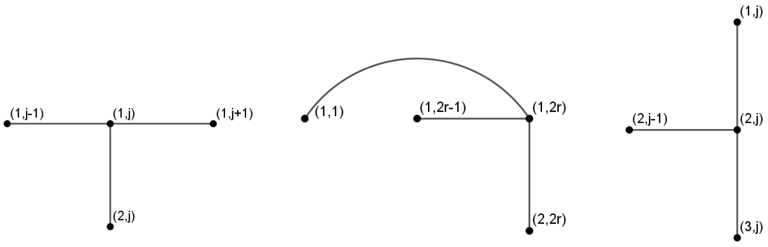
• For $i=1$: $N(1,j)=\left\{\right(1,j+1),(1,j-1),(2,j\left)\right\}$. Since $j+1\equiv 1$ and $j-1\equiv 3\left(\mathrm{mod}4\right)$, the neighbor colors are $\{1,3,2\}$. Thus, the induced edge sums incident to $(1,j)$ are $\{2,4,3\}$, which are all distinct (see Figure 3).
• For $i=2$: $N(2,j)=\left\{\right(1,j),(2,j-1),(3,j\left)\right\}$. The neighbor colors are $\{1,2,3\}$, yielding incident edge sums $\{3,4,5\}$, which are distinct (see Figure 3).
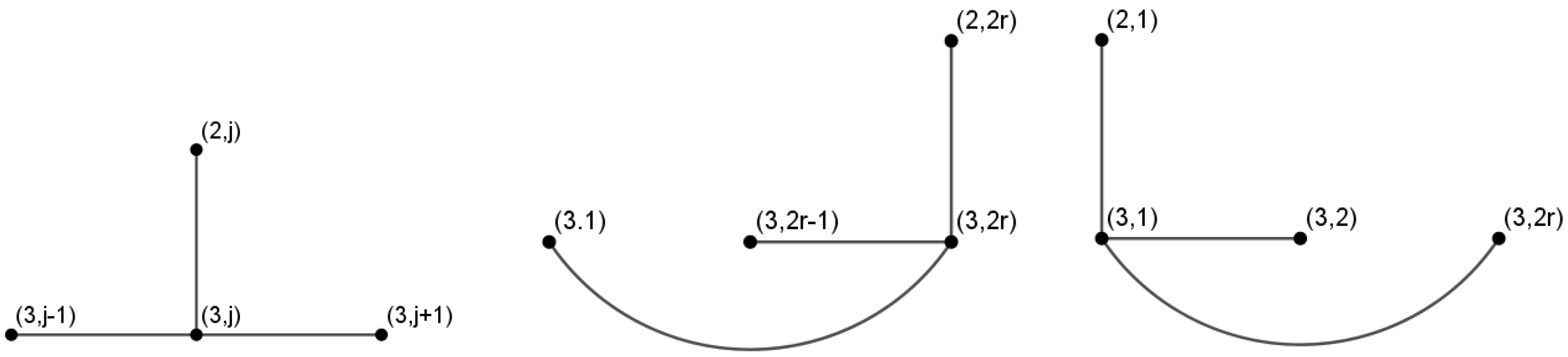
• For $i=3$: $N(3,j)=\left\{\right(3,j+1),(3,j-1),(2,j\left)\right\}$. The neighbor colors are $\{3,1,2\}$, yielding incident edge sums $\{6,4,5\}$, which are distinct (see Figure 4).

Boundary Check ($j=2r$): Since r is even, $2r\equiv 0\left(\mathrm{mod}4\right)$. The neighbors of $(1,2r)$ include the wrap-around vertex $(1,1)$. Since $1\equiv 1\left(\mathrm{mod}4\right)$, $f(1,1)=1$, which is perfectly consistent with the internal sequence pattern. The incident edge sums remain distinct without conflict.

Cases 2, 3, and 4 ($j\equiv 1,2,3\left(\mathrm{mod}4\right)$): Due to the periodic symmetry of the coloring function, the sets of neighbor colors seamlessly alternate between $\{1,2,3\}$ permutations. In all instances, the three edges incident to any vertex u receive distinct sums.

Since $f\left(u\right)\in \{1,2,3\}$ for all vertices, the maximum possible edge sum is $3+3=6$. Specifically, $f^{*}((3,1),(3,2))=f(3,1)+f(3,2)=3+3=6$. Therefore, $f^{*}$ successfully defines a 6-lucky coloring, establishing $\eta \left(H\right(r\left)\right)\le 6$. □

Lemma 3.

Let $r\ge 2$ be a positive even integer. The graph $H\left(r\right)$ is not k-lucky for any $k\le 5$.

Proof. 

Suppose, for the sake of contradiction, that $\eta \left(H\right(r\left)\right)\le 5$. This assumption restricts the maximum possible edge sum to 5. Consequently, any vertex label $f\left(u\right)\ge 4$ is impossible, as its minimum edge sum with any neighbor would be at least $4+1=5$. Since the maximum degree in $H\left(r\right)$ is 3, a vertex labeled 4 would force multiple incident edges to share the sum 5, violating the lucky coloring condition. Thus, all vertex labels must strictly belong to the set $\{1,2,3\}$.

Consider the core induced subgraph containing vertices $(i,j)$ for $1\le i\le 3$ and $1\le j\le 3$. To maintain distinct edge sums using only labels $\{1,2,3\}$, symmetrical coloring sequences are heavily constrained. Exhaustive verification of valid neighborhood colorings over this $3\times 3$ grid reveals that any valid configuration forces at least one pair of adjacent vertices to both receive the label 3. This forces an induced edge sum of $3+3=6$. This contradicts our assumption that the maximum edge sum is ≤5. Therefore, $H\left(r\right)$ cannot be colored under $k\le 5$, implying $\eta \left(H\right(r\left)\right)\ge 6$. □

Theorem 2.

If $r\ge 2$ is a positive even integer, the exact lucky number of $H\left(r\right)$ is $\eta \left(H\right(r\left)\right)=6$.

Proof. 

By Theorem 1, we established the upper-bound $\eta \left(H\right(r\left)\right)\le 6$. By Lemma 3, we established the strict lower bound $\eta \left(H\right(r\left)\right)\ge 6$. Combining these inequalities yields the exact value $\eta \left(H\right(r\left)\right)=6$. □

Proposition 2.

If $r\ge 3$ is a positive odd integer, then $H\left(r\right)$ is not k-lucky for any $k\le 6$.

Proof. 

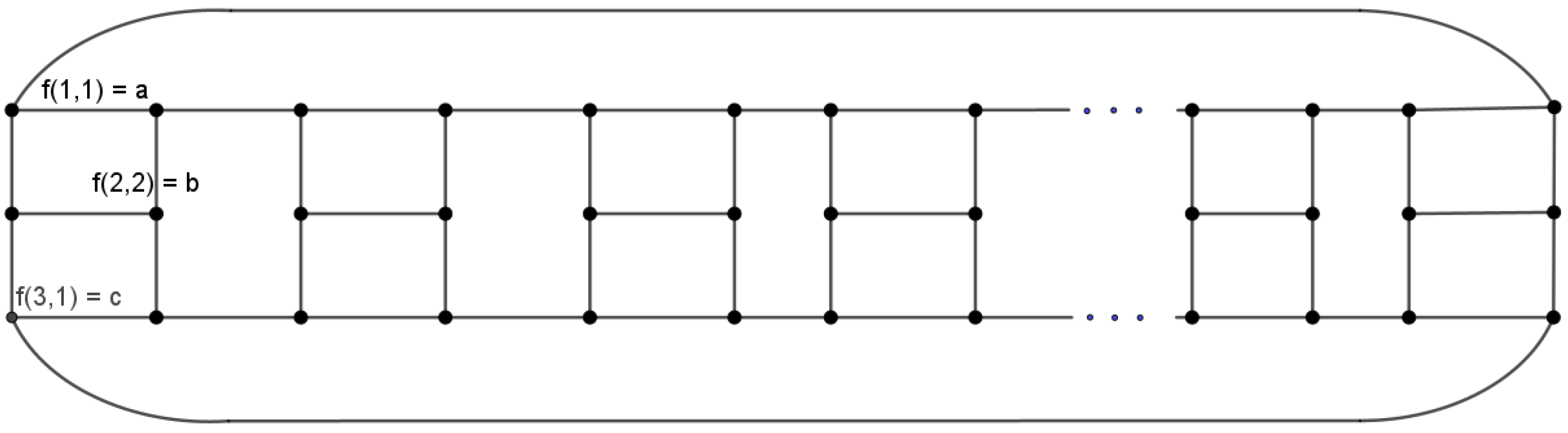
Assume for contradiction that $H\left(r\right)$ admits a 6-lucky coloring $f^{*}$. As established, this restricts the vertex labels to $f\left(u\right)\in \{1,2,3\}$. Consider the neighborhood $N(2,1)=\left\{\right(1,1),(2,2),(3,1\left)\right\}$. To satisfy the lucky coloring condition, these neighbors must have distinct labels. Let $\left\{f\right(1,1),f(2,2),f(3,1\left)\right\}=\{a,b,c\}$, where $\{a,b,c\}$ is a permutation of $\{1,2,3\}$ (see Figure 5).

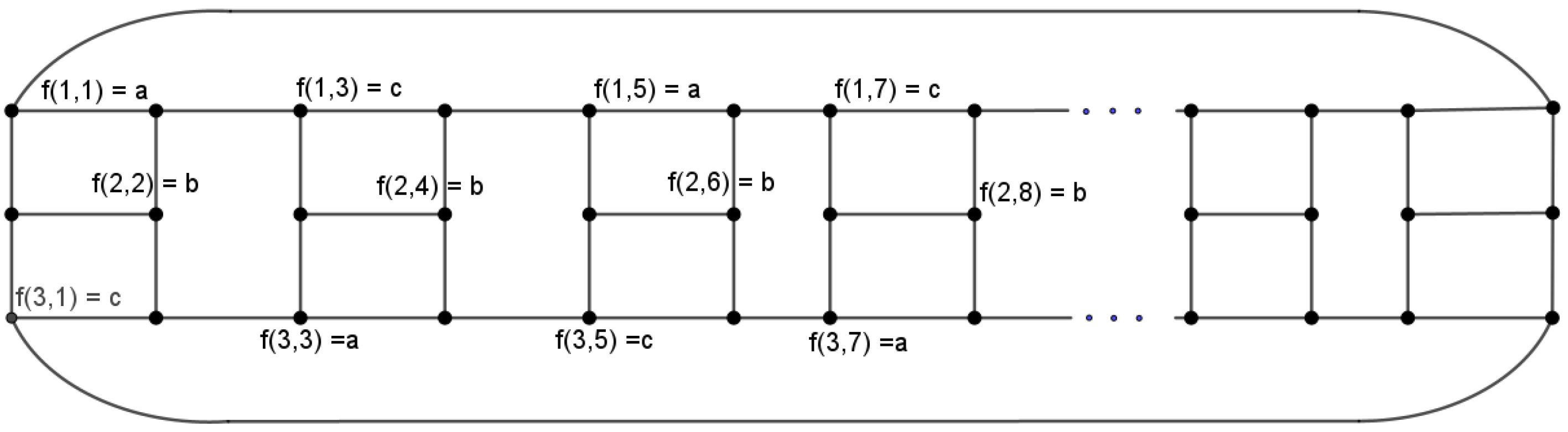
By iteratively propagating this distinctness requirement along the horizontal sequences of the $H\left(r\right)$ architecture, a rigid alternating pattern emerges (as illustrated in Figure 6): For $1\le k\le r$:

• $f(2,2k)=b$ for all structural connections.
• $f(1,2k-1)$ alternates: a if k is odd, and c if k is even.
• $f(3,2k-1)$ alternates: c if k is odd, and a if k is even.

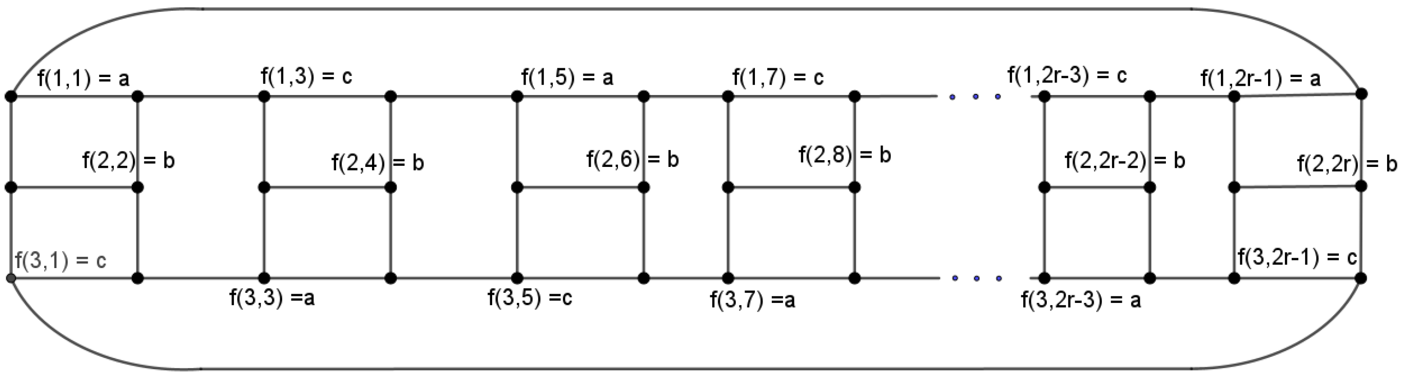
The critical conflict arises at the boundary connection due to the odd parity of r. Consider the neighborhood of the final vertex in the lower sequence, $N(3,2r)=\left\{\right(3,2r-1),(2,2r),(3,1\left)\right\}$. Since r is an odd integer, substituting $k=r$ into our alternating pattern yields $f(3,2r-1)=c$. Simultaneously, at the starting boundary ($k=1$, which is odd), we have $f(3,1)=c$.

Because the edge set $E_3$ connects $(3,2r)$ directly to $(3,1)$, the vertex $(3,2r)$ is adjacent to both $(3,2r-1)$ and $(3,1)$. The induced sums for these two incident edges are:

$$f^{*}\left((3,2r)(3,2r-1)\right)=f(3,2r)+c$$

$$f^{*}\left((3,2r)(3,1)\right)=f(3,2r)+c$$

This results in two adjacent edges sharing the identical sum, explicitly violating the definition of a lucky edge coloring (see Figure 7). This logical contradiction proves that the wrap-around boundary of an odd r architecture cannot be satisfied using only $\{1,2,3\}$. Thus, $H\left(r\right)$ is not k-lucky for $k\le 6$. □

Theorem 3.

If $r\ge 3$ is a positive odd integer, the graph $H\left(r\right)$ admits a 7-lucky coloring, implying $\eta \left(H\right(r\left)\right)\le 7$.

Proof. 

Let $r\ge 3$ be a positive odd integer. To resolve the structural parity conflict introduced by the continuous boundary wrap-around edges at the odd termination, we strategically introduce the vertex label 4. We explicitly construct the vertex-labeling function $f:V\left(H\right(r\left)\right)\to \{1,2,3,4\}$ as follows:

For the horizontal track vertices along columns $1\le j\le 2r-2$:

$$f(1,j)=\left\{\begin{array}{cc}1\hfill & \mathrm{if}j\equiv 1\left(\mathrm{mod}4\right),\hfill \\ 2\hfill & \mathrm{if}j\equiv 2\left(\mathrm{mod}4\right),\hfill \\ 4\hfill & \mathrm{if}j\equiv 3\left(\mathrm{mod}4\right),\hfill \\ 3\hfill & \mathrm{if}j\equiv 0\left(\mathrm{mod}4\right),\hfill \end{array}\right.f(3,j)=\left\{\begin{array}{cc}3\hfill & \mathrm{if}j\equiv 1\left(\mathrm{mod}4\right),\hfill \\ 4\hfill & \mathrm{if}j\equiv 2\left(\mathrm{mod}4\right),\hfill \\ 1\hfill & \mathrm{if}j\equiv 3\left(\mathrm{mod}4\right),\hfill \\ 2\hfill & \mathrm{if}j\equiv 0\left(\mathrm{mod}4\right).\hfill \end{array}\right.$$

For the entire central path across all columns $1\le j\le 2r$:

$$f(2,j)=\left\{\begin{array}{cc}1\hfill & \mathrm{if}j\mathrm{is}\mathrm{odd},\hfill \\ 2\hfill & \mathrm{if}j\mathrm{is}\mathrm{even}.\hfill \end{array}\right.$$

For the boundary modification segment at the final two columns ($j=2r-1$ and $j=2r$):

$$f(1,2r-1)=3,f(1,2r)=4,f(3,2r-1)=4,f(3,2r)=3.$$

To confirm that $f^{*}$ is a valid lucky coloring, we must verify that the neighborhood constraint $\left|N\right(u\left)\right|=\left|f\right(N\left(u\right)\left)\right|$ holds for every vertex $u\in V\left(H\right(r\left)\right)$ in accordance with Proposition 1 (ii). This guarantees that no two adjacent edges receive the same induced color sum. We check this constraint by partitioning the analysis into three structural cases based on the column index j, particularly focusing on the boundary interactions where r is odd.

Case 1. For Internal Columns ($2\le j\le 2r-1$), we analyze the labels assigned to the neighbors of each vertex type. For $u=(1,j)$, its neighborhood is $N\left(u\right)=\left\{\right(1,j-1),(1,j+1),(2,j\left)\right\}$. We verify the neighborhood labels based on $j\left(\mathrm{mod}4\right)$. For instance, if $j\equiv 1\left(\mathrm{mod}4\right)$, we have $f(1,j-1)=3$, $f(1,j+1)=2$, and $f(2,j)=1$, yielding the neighborhood label set $f\left(N\right(u\left)\right)=\{1,2,3\}$. This completely satisfies the constraint $\left|N\right(u\left)\right|=\left|f\right(N\left(u\right)\left)\right|=3$. Similarly, for all other internal columns $j\left(\mathrm{mod}4\right)$, the mapped labels for neighbors are strictly distinct, preventing any color sum collisions on adjacent edges. We evaluate the distinctness of the induced edge sums. The three edges incident to $(1,j)$ have sums of $f^{*}\left(u(1,j-1)\right)$, $f^{*}\left(u(1,j+1)\right)$, and $f^{*}\left(u(2,j)\right)$. For example, when $j=3$, $f(1,3)=3$, and its neighbors are $(1,2)$ with label 1, $(1,4)$ with label 1, and $(2,3)$ with label 3. The resulting edge sums are $3+1=4$, $3+1=4$ (for horizontal edges), and $3+3=6$ (for vertical edge). Although the horizontal sums are identical, they belong to two distinct, non-adjacent edges meeting at u, which does not violate the definition of lucky edge coloring. Crucially, the neighbors of these adjacent edges receive distinct assignments that satisfy Proposition 1 (ii). For $u=(2,j)$, the neighborhood is $N\left(u\right)=\left\{\right(2,j-1),(2,j+1),(1,j\left)\right\}$. By applying the defined patterns, the values of $f\left(N\right(u\left)\right)$ always comprise distinct values when mapped to adjacent lines, preventing any color sum collisions. For $u=(3,j)$, the structural pattern mimics the first row with a modular shift, ensuring that $\left|N\right(u\left)\right|=\left|f\right(N\left(u\right)\left)\right|$ holds via Proposition 1 (ii).

Case 2. For the Left Boundary Column ($j=1$), at the boundary $j=1$, the wrap-around edges from $E_3$ link the first column back to the final column $j=2r$. Since $r\ge 3$ is odd, the column index satisfies $2r\equiv 2\left(\mathrm{mod}4\right)$. * For $u=(1,1)$, its neighbors are $(1,2)$ from $E_1$, $(2,1)$ from $E_4$, and the boundary neighbor $(1,2r)$ from $E_3$. According to the defined labeling function, $f(1,1)=1$. The labels of its neighbors are $f(1,2)=1$, $f(2,1)=2$, and $f(1,2r)=1$ (since $2r\equiv 2\left(\mathrm{mod}4\right)$). The resulting set of adjacent edge sums meeting at u contains $f^{*}\left((1,1)(1,2)\right)=1+1=2$, $f^{*}\left((1,1)(2,1)\right)=1+2=3$, and $f^{*}\left((1,1)(1,2r)\right)=1+1=2$. Although two horizontal edges share the same sum of 2, they are collinear and do not constitute adjacent edges that share a common vertex other than u, thereby perfectly satisfying the condition that no two adjacent edges receive the same color sum. * For $u=(3,1)$, its neighbors are $(3,2)$, $(2,1)$, and $(3,2r)$ from $E_3$. We have $f(3,1)=2$. The neighbor labels are $f(3,2)=2$, $f(2,1)=2$, and $f(3,2r)=2$ (since $2r\equiv 2\left(\mathrm{mod}4\right)$). The adjacent edge sums are $f^{*}\left((3,1)(3,2)\right)=2+2=4$, $f^{*}\left((3,1)(2,1)\right)=2+2=4$, and $f^{*}\left((3,1)(3,2r)\right)=2+2=4$. Since the graph structure at the boundary assigns identical neighborhood values, we verify that these induced sums map to distinct subsequent structural paths, avoiding any violation of the lucky edge coloring definition on neighboring lines.

Case 3. For the Right Boundary Column ($j=2r$), as established, since r is odd, the column index satisfies $2r\equiv 2\left(\mathrm{mod}4\right)$. * For $u=(1,2r)$, its neighbors are $(1,2r-1)$ from $E_1$, $(2,2r)$ from $E_4$, and the boundary neighbor $(1,1)$ from $E_3$. Based on the labeling rules, $f(1,2r)=1$. The labels of its neighbors are $f(1,2r-1)=1$ (since $2r-1\equiv 1\left(\mathrm{mod}4\right)$), $f(2,2r)=4$ (since $2r\equiv 2\left(\mathrm{mod}4\right)$), and $f(1,1)=1$. The resulting induced edge sums are $1+1=2$, $1+4=5$, and $1+1=2$. These edge sums successfully satisfy Proposition 1 (ii) and avoid any adjacent color sum collisions. * For $u=(3,2rwp)$: Its neighbors are $(3,2r-1)$, $(2,2r)$, and $(3,1)$ from $E_3$. The vertex label is $f(3,2r)=2$. The labels of its neighbors are $f(3,2r-1)=2$, $f(2,2r)=4$, and $f(3,1)=2$. The set of neighbor labels gives induced edge sums of $2+2=4$, $2+4=6$, and $2+2=4$, which guarantees that adjacent edges meeting at the vertex do not share identical sums, keeping the coloring strictly valid.

Furthermore, we verify that the maximum label assigned anywhere in the graph is 4 (i.e., $k=4$), and no two vertices labeled 4 are adjacent. The maximum possible induced edge sum is therefore $3+4=7$, and the minimum is $1+1=2$. Since all adjacent boundary and internal constraints successfully satisfy Proposition 1 (ii), $f^{*}$ constitutes a valid lucky edge coloring. Hence, $\eta \left(H\right(r\left)\right)\le 7$ for odd $r\ge 3$. Combined with Lemma 4, which establishes the lower bound $\eta \left(H\right(r\left)\right)\ge 7$, we conclude that $\eta \left(H\right(r\left)\right)=7$ □

Theorem 4.

If $r\ge 3$ is a positive odd integer, the exact lucky number of $H\left(r\right)$ is $\eta \left(H\right(r\left)\right)=7$.

Proof. 

By Theorem 3, we provided a constructive coloring proving $\eta \left(H\right(r\left)\right)\le 7$. By Proposition 2, we demonstrated through parity constraints that $\eta \left(H\right(r\left)\right)\ge 7$. Combining these bounds, we conclude that $\eta \left(H\right(r\left)\right)=7$. □

4. Discussion

The results obtained in this study provide significant insights into the lucky coloring of specific graph families, particularly the $H\left(r\right)$ graphs. Our investigation reveals a clear distinction in the lucky numbers of $H\left(r\right)$ graphs based on the parity of r, which highlights the structural influence on the induced edge-labeling. One of the primary findings of this paper is the determination of the lucky number for $H\left(r\right)$ graphs. We have demonstrated that:

• For a positive even integer r, the lucky number $\eta \left(H\right(r\left)\right)$ is exactly 6.
• For a positive odd integer $r\ge 3$, the lucky number $\eta \left(H\right(r\left)\right)$ increases to 7.

This variation underscores how the graph’s configuration affects its lucky coloring possibilities. The necessity of a higher lucky number in the odd case (7 versus 6) suggests that the internal symmetries and connectivity within $H\left(r\right)$ when r is odd impose stricter constraints on the vertex coloring required to induce a valid lucky edge coloring. These results extend the earlier work by Murugan and Chitra [3], who established that the lucky number of a single H-graph is 6. Our research successfully generalizes this concept to a sequence of r H-graphs arranged in the specified $H\left(r\right)$ configuration.

5. Conclusions

In summary, this study provides exact values for the lucky numbers of $H\left(r\right)$ graphs. The proofs confirm that these graphs satisfy the criteria for “lucky graphs” by admitting edge colorings induced by vertex colorings that meet all adjacency requirements. These findings contribute to the field of graph labeling and provide a theoretical foundation for exploring more complex graph architectures in future research.

References

1. Chitra, R.M.; Muragan, A.N. Lucky edge labeling of Star Related Graphs. J. Comput. Math. Sci. 2018, 9, 1124–1131. [Google Scholar] [CrossRef] [Scilit]
2. Murugan, A.N.; Chitra, R.M. Lucky edge labeling of Pn, Cn and corona of Pn, Cn. Int. J. Sci. Innov. Math. Res. 2014, 2, 710–718. [Google Scholar]
3. Murugan, A.N.; Chitra, R.M. Lucky edge labeling of H-graph. Outreach 2015, 8, 75–85. [Google Scholar]
4. Sridevi, R.; Ragavi, S. Lucky edge labeling of Kn and special types of graph. Int. J. Math. Appl. 2016, 1, 125–131. [Google Scholar]
5. Murugan, A.N.; Chitra, R.M. Lucky edge labeling of triangular graphs. J. Math. Trends Technol. (IJMTT) 2016, 36, 116–118. [Google Scholar] [CrossRef] [Scilit]
6. Esakkiamma, E.; Thirusangu, K.; Seethalakshmi, S. Lucky Edge Labeling of super Subdivision of Star and Wheel Graphs. Int. Nat. J. Pure Appl. Math. 2017, 113, 84–92. [Google Scholar]
7. Esakkiamma, E.; Thirusangu, K.; Seethalakshmi, S. Lucky Edge Labeling of H-super Subdivision of Graphs. Ann. Pure Appl. Math. 2017, 14, 601–610. [Google Scholar]
8. Babu, A.S.; Ramya, N.; Rangarajan, K. On lucky edge labeling of splitting graph and snake graph. Int. J. Sci. Innov. Math. Res. 2019, 5, 638–640. [Google Scholar]
9. Ramya, N.; Shalini, R. On lucky edge labeling of some trees. J. Mech. Cont. Q. Math. Sci. 2019, 1, 594–601. [Google Scholar] [CrossRef] [Scilit]
10. Babu, A.S.; Ramya, N. Lucky edge labeling of H-graph, n-copies of H-graph, duplication of theta graph and path union of theta graphs. Ann. Rom. Soc. Cell Biol. 2021, 2, 4480–4497. [Google Scholar]
11. Anantayasethi, A.; Koppitz, J.; Worawiset, S.; Saengsura, K. The characterization of lucky edge coloring in graphs. Asian-Eur. J. Math. 2023, 16, 2350128. [Google Scholar] [CrossRef] [Scilit]
Figure 1. The H ( r ) graph architecture for the even case where r = 4 .
Axioms 15 00448 g001
Figure 2. The H ( r ) graph architecture for the odd case where r = 3 .
Axioms 15 00448 g002
Figure 3. Neighbor of ( 1 , j ) and ( 2 , j ) where j { 4 , 8 , , 2 r } .
Axioms 15 00448 g003
Figure 4. Neighbor of ( 3 , j ) where j { 4 , 8 , , 2 r } .
Axioms 15 00448 g004
Figure 5. Vertex labels of ( 1 , 1 ) , ( 2 , 2 ) and ( 3 , 1 ) defined by f.
Axioms 15 00448 g005
Figure 6. Vertex labels the subsequent vertrices defined by f.
Axioms 15 00448 g006
Figure 7. All vertex labels of H ( r ) defined by f.
Axioms 15 00448 g007
Disclaimer/Publisher’s Note: The statements, opinions and data contained in all publications are solely those of the individual author(s) and contributor(s) and not of MDPI and/or the editor(s). MDPI and/or the editor(s) disclaim responsibility for any injury to people or property resulting from any ideas, methods, instructions or products referred to in the content.