About a Problem of Stabilization by Noise for a System of Linear Differential Equations

Abstract

The well-known effect of stabilization by noise for Ito’s scalar linear stochastic differential equation was proven by R.Z. Khasminskii more than 50 years ago. Here, a similar statement is obtained for a system of linear stochastic differential equations. The obtained result is illustrated on the system of two linear stochastic differential equations via several special examples with numerical simulations and figures.

1. Introduction

More than 50 years ago, R.Z. Khasminskii showed [1] that the zero solution of the scalar linear stochastic differential Equation [2],

$$dx\left(t\right)=ax\left(t\right)dt+\sigma x\left(t\right)dw\left(t\right),$$

(1)

which is evidently unstable by $a>0$ and $\sigma =0$, becomes stable in probability by a sufficiently large level of noise, i.e., by the condition

$${\sigma }^2>2a.$$

(2)

During the next years research on this so-called effect of stabilization via noise was continued and developed in many other works (see, for instance, [3,4,5,6,7,8,9,10,11,12]).

Below, a new result in this direction is obtained for the system of linear stochastic differential equations [2]

$$dx\left(t\right)=Ax\left(t\right)dt+{\displaystyle \sum _{i=1}^n}{S}_{i}x\left(t\right)d{w}_i\left(t\right),$$

(3)

where $x\left(t\right)\in {\mathbf{R}}^{\mathbf{n}}$, $A,S_i\in {\mathbf{R}}^{\mathbf{n}\times \mathbf{n}}$, $w_1\left(t\right),\dots ,w_n\left(t\right)$ are mutually independent Wiener processes, by the condition that the zero solution of the deterministic linear differential equation

$$\dot{x}\left(t\right)=Ax\left(t\right)$$

(4)

is unstable.

It is known [1] that for asymptotic stability of the zero solution of Equation (4), the matrix A must satisfy the condition

$$Tr\left(A\right)<0.$$

(5)

Here, the conditions of stability in probability of the zero solution of Equation (3) are obtained under the assumption that the condition (5) does not hold, i.e., the zero solution of the deterministic linear Equation (4) is unstable. Some particular cases of this statement are considered and illustrated via special examples with numerical simulation of solutions of the system of stochastic differential equations and figures.

2. Stability

Let $\{\mathsf{\Omega },\mathfrak{F},\mathbf{P}\}$ be a complete probability space, $\{{\mathfrak{F}}_t,t\ge 0\}$ be a nondecreasing family of sub-$\sigma$-algebras of $\mathfrak{F}$, i.e., ${\mathfrak{F}}_{t_1}\subset {\mathfrak{F}}_{t_2}\subset \mathfrak{F}$ for $t_1<t_2$, and $\mathbf{E}$ be the mathematical expectation with respect to the measure $\mathbf{P}$.

Definition 1.

The solution $x\left(t\right)$ of Equation (3) is called stable in probability if for any ${\epsilon }_1>0$ and ${\epsilon }_2>0$, there exists $\delta >0$ such that $x\left(t\right)$ satisfies the condition $\mathbf{P}\{\underset{t\ge 0}{\sup }\left|x\left(t\right)\right|>{\epsilon }_1\} <{\epsilon }_2$ for any $x\left(0\right)$ such that $\mathbf{P}\left\{\right|x\left(0\right)|<\delta \}=1$.

Remark 1.

Let the function $V\left(x\right)$, $x\in {\mathbf{R}}^n$, have two derivatives, $\nabla V\left(x\right)$ and ${\nabla }^{2}V\left(x\right)$. The generator L of Equation (3) has the form [2,13]

$$LV\left(x\right)={(\nabla V\left(x\right))}^{\prime }Ax+{\displaystyle \frac{1}{2}}{\displaystyle \sum _{i=1}^n}{x}^{\prime }{S}_i{\nabla }^{2}V\left(x\right)S_{i}x,$$

(6)

where "′" is the sign of transposition, and $\nabla V\left(x\right)$ and ${\nabla }^{2}V\left(x\right)$ are, respectively, the vector of the first derivatives and the matrix of the second derivatives of the function $V\left(x\right)$.

Theorem 1.

[1,13] Let there exist a Lyapunov function $V\left(x\right)$ for which $LV\left(x\right)\le 0$. Then the zero solution of Equation (3) is stable in probability.

Theorem 2.

Let there exist a positive definite matrix $P\in {\mathbf{R}}^{\mathbf{n}\times \mathbf{n}}$ and a number $\nu \in (0,1)$ for which the matrix

$$Q=PA+A^{\prime }P-\nu {\displaystyle \sum _{i=1}^n}{S}_i^{\prime }P{S}_i$$

(7)

satisfies the condition $x^{\prime }Qx\le 0$. Then the zero solution of Equation (3) is stable in probability.

Proof. 

Following Theorem 1, it is enough to show that there exists some Lyapunov function $V\left(x\right)$, for which the condition $LV\left(x\right)\le 0$ holds.

Consider the Lyapunov function $V\left(x\right)={\left(x^{\prime }Px\right)}^{\mu }$ with $\mu =0.5(1-\nu )$ and note that

$$\begin{gathered} \nabla V\left(x\right)=2\mu {\left(x^{\prime }Px\right)}^{\mu -1}Px, \\ {\nabla }^{2}V\left(x\right)=2\mu {\left(x^{\prime }Px\right)}^{\mu -1}P+4\mu (\mu -1){\left(x^{\prime }Px\right)}^{\mu -2}P\left(x{x}^{\prime }\right)P. \end{gathered}$$

(8)

From (6) and (8), we obtain

$$\begin{gathered} LV\left(x\right)=2\mu {\left(x^{\prime }Px\right)}^{\mu -1}\left(x^{\prime }PAx\right)+\mu {\left(x^{\prime }Px\right)}^{\mu -1}{\displaystyle \sum _{i=1}^n}{x}^{\prime }{S}_i^{\prime }P{S}_{i}x \\ +2\mu (\mu -1){\left(x^{\prime }Px\right)}^{\mu -2}{\displaystyle \sum _{i=1}^n}{x}^{\prime }{S}_i^{\prime }P\left(x{x}^{\prime }\right)P{S}_{i}x \\ =\mu {\left(x^{\prime }Px\right)}^{\mu -1}{x}^{\prime }\left(PA+A^{\prime }P+{\displaystyle \sum _{i=1}^n}{S}_i^{\prime }P{S}_i\right)x \\ +2\mu (\mu -1){\left(x^{\prime }Px\right)}^{\mu -2}{\displaystyle \sum _{i=1}^n}{\left(x^{\prime }{S}_i^{\prime }Px\right)}^2. \end{gathered}$$

(9)

Using the inequality ${\left(a^{\prime }b\right)}^2\le {\left|a\right|}^2{\left|b\right|}^2$, we have

$${\left(x^{\prime }{S}_i^{\prime }Px\right)}^2={\left(x^{\prime }{S}_i^{\prime }{P}^{0.5}{P}^{0.5}x\right)}^2\le \left(x^{\prime }{S}_i^{\prime }P{S}_{i}x\right)\left(x^{\prime }Px\right).$$

So,

$${\left(x^{\prime }Px\right)}^{\mu -2}{\displaystyle \sum _{i=1}^n}{\left(x^{\prime }{S}_i^{\prime }Px\right)}^2\le {\left(x^{\prime }Px\right)}^{\mu -1}{\displaystyle \sum _{i=1}^n}\left(x^{\prime }{S}_i^{\prime }P{S}_{i}x\right).$$

(10)

As a result, substituting (10) into (9) and using (7) with $2\mu -1=-\nu$, we obtain

$$\begin{gathered} LV\left(x\right)\le \mu {\left(x^{\prime }Px\right)}^{\mu -1}{x}^{\prime }\left(PA+A^{\prime }P+{\displaystyle \sum _{i=1}^n}{S}_i^{\prime }P{S}_i+2(\mu -1){\displaystyle \sum _{i=1}^n}{S}_i^{\prime }P{S}_i\right)x \\ =\mu {\left(x^{\prime }Px\right)}^{\mu -1}{x}^{\prime }Qx\le 0. \end{gathered}$$

The proof is completed. □

Remark 2.

Note that for the scalar Equation (1), the condition on the matrix (7) takes the form $2a\le \nu {\sigma }^2<{\sigma }^2$, i.e., coincides with (2). Below, the matrix (7) is used for getting necessary conditions on the parameters of a considered system of linear stochastic differential equations.

3. System of Two Equations

Consider the system of two linear equations

$$\begin{gathered} d{x}_1=(a_{11}{x}_1+a_{12}{x}_2)dt+{\sigma }_1{x}_{1}d{w}_1\left(t\right), \\ d{x}_2=(a_{21}{x}_1+a_{22}{x}_2)dt+{\sigma }_2{x}_{2}d{w}_2\left(t\right). \end{gathered}$$

(11)

Theorem 3.

Let the following conditions hold:

$${\sigma }_1^2>2a_{11}>0,{\sigma }_2^2>2a_{22}>0,a_{12}{a}_{21}\le 0.$$

(12)

Then the zero solution of the system (11) is stable in probability.

Proof. 

For the beginning note, by the condition $a_{12}=a_{21}=0$, the system (11) splits into two independent equations, for which the condition of stability in probability is known and coincides with (12) [13].

In the general case, let us construct the matrix (7) for the system (11), using the diagonal matrix P. In this case,

$$PA=\left\{\begin{array}{cc}{p}_{11}& 0\\ 0& p_{22}\end{array}\right\}\left\{\begin{array}{cc}{a}_{11}& a_{12}\\ a_{21}& a_{22}\end{array}\right\}=\left\{\begin{array}{cc}{p}_{11}{a}_{11}& p_{11}{a}_{12}\\ p_{22}{a}_{21}& p_{22}{a}_{22}\end{array}\right\}.$$

Note also that for the system (11), the matrices $S_1$ and $S_2$ take the forms

$$S_1=\left\{\begin{array}{cc}{\sigma }_1& 0\\ 0& 0\end{array}\right\},S_1=\left\{\begin{array}{cc}0& 0\\ 0& {\sigma }_2\end{array}\right\}.$$

So, via (7), we obtain

$$Q=\left\{\begin{array}{cc}(2a_{11}-\nu {\sigma }_1^2)p_{11}& p_{11}{a}_{12}+p_{22}{a}_{21}\\ p_{11}{a}_{12}+p_{22}{a}_{21}& (2a_{22}-\nu {\sigma }_2^2)p_{22}\end{array}\right\}.$$

Note that the matrix Q is negative definite if $Tr\left(Q\right)<0$ and $\det \left(Q\right)>0$. By the conditions (12), there exists $\nu$ such that

$$2a_{11}<\nu {\sigma }_1^2,2a_{22}<\nu {\sigma }_2^2,\nu \in (0,1),$$

$$(2a_{11}-\nu {\sigma }_1^2)(2a_{22}-\nu {\sigma }_2^2)p_{11}{p}_{22}>{(p_{11}{a}_{12}+p_{22}{a}_{21})}^2.$$

(13)

To prove stability in probability of the system (11), let us note that for all possible cases of the condition $a_{12}{a}_{21}\le 0$, the matrix P, for which the condition (13) holds, the following exists:

-

It is clear in the case $a_{12}=a_{21}=0$;

-

If $a_{12}=0$ and $a_{21}\ne 0$, then $(2a_{11}-\nu {\sigma }_1^2)(2a_{22}-\nu {\sigma }_2^2)p_{11}>p_{22}{a}_{21}^2$ with small enough $p_{22}$, and similarly if $a_{12}\ne 0$ and $a_{21}=0$ with small enough $p_{11}$;

-

If $a_{12}{a}_{21}<0$, then $p_{11}$ and $p_{22}$ can be chosen such that ${\displaystyle \frac{p_{11}}{p_{22}}}=\left|{\displaystyle \frac{a_{21}}{a_{12}}}\right|$, i.e., $p_{11}{a}_{12}+p_{22}{a}_{21}=0$.

The proof is completed. □

4. Examples

Note that from the condition (12) it follows that for the system (11) $Tr\left(A\right)=a_{11}+a_{22}>0$, i.e., the condition (5) does not hold. Consider some relevant examples.

Example 1.

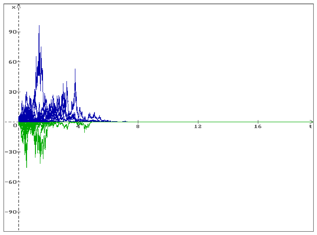
Let be $a_{11}=0.5$, $a_{12}=0$, $a_{21}=0$, $a_{22}=0.7$, ${\sigma }_1=4$, ${\sigma }_2=5$, $x_1\left(0\right)=2$, $x_2\left(0\right)=-1$. In this case, both equations of the system (11) are independent of each other. Furthermore, the solution of the first equation with a positive initial condition remains positive (blue), and the solution of the second equation with a negative initial condition remains negative (green) (see Figure 1). The zero solution of the system (11) is stable in probability, so all trajectories converge to zero.

Example 2.

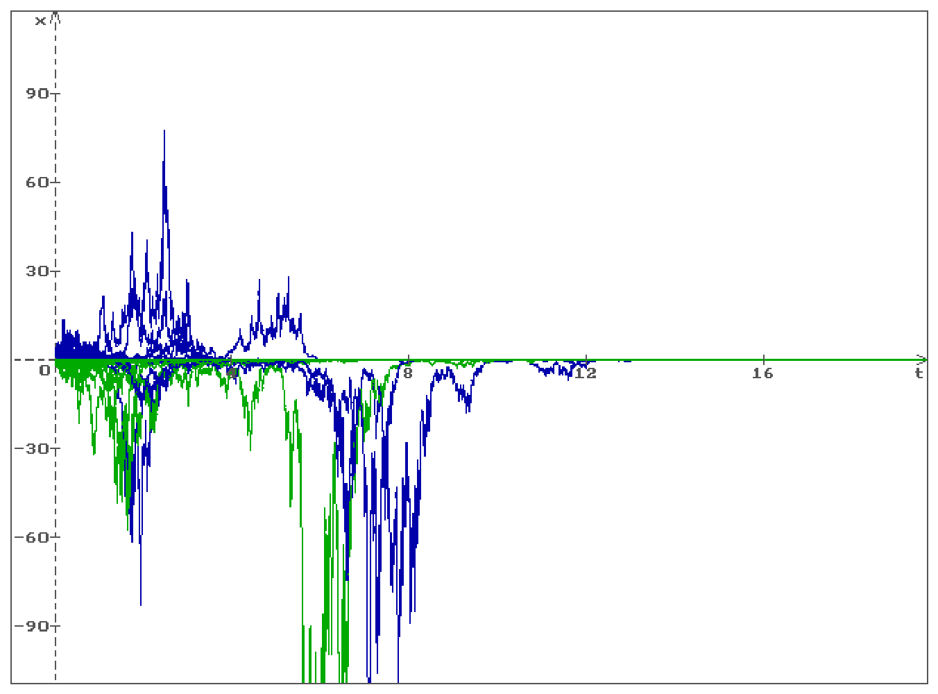
Let be $a_{11}=0.5$, $a_{12}=0.25$, $a_{21}=0$, $a_{22}=0.5$, ${\sigma }_1=4$, ${\sigma }_2=4$, $x_1\left(0\right)=2$, $x_2\left(0\right)=-1$. In this case, the second equation of the system (11) is independent of the first one; the solution of the second equation with a negative initial condition remains negative (green), and the solution of the first equation with a positive initial condition has both positive and negative values (blue) (see Figure 2). The zero solution is stable in probability, so all trajectories converge to zero.

Example 3.

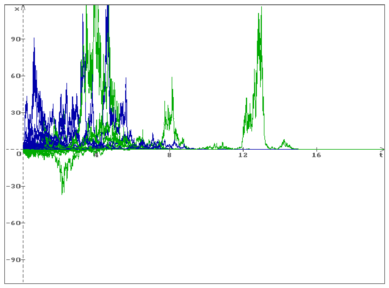
Let be $a_{11}=0.5$, $a_{12}=0$, $a_{21}=0.25$, $a_{22}=0.5$, ${\sigma }_1=4$, ${\sigma }_2=4$, $x_1\left(0\right)=2$, $x_2\left(0\right)=-1$. In this case, the first equation of the system (11) is independent of the second one; the solution of the first equation with a positive initial condition remains positive (blue), and the solution of the second equation with a negative initial condition has both negative and positive values (green) (see Figure 3). The zero solution is stable in probability, so all trajectories converge to zero.

Example 4.

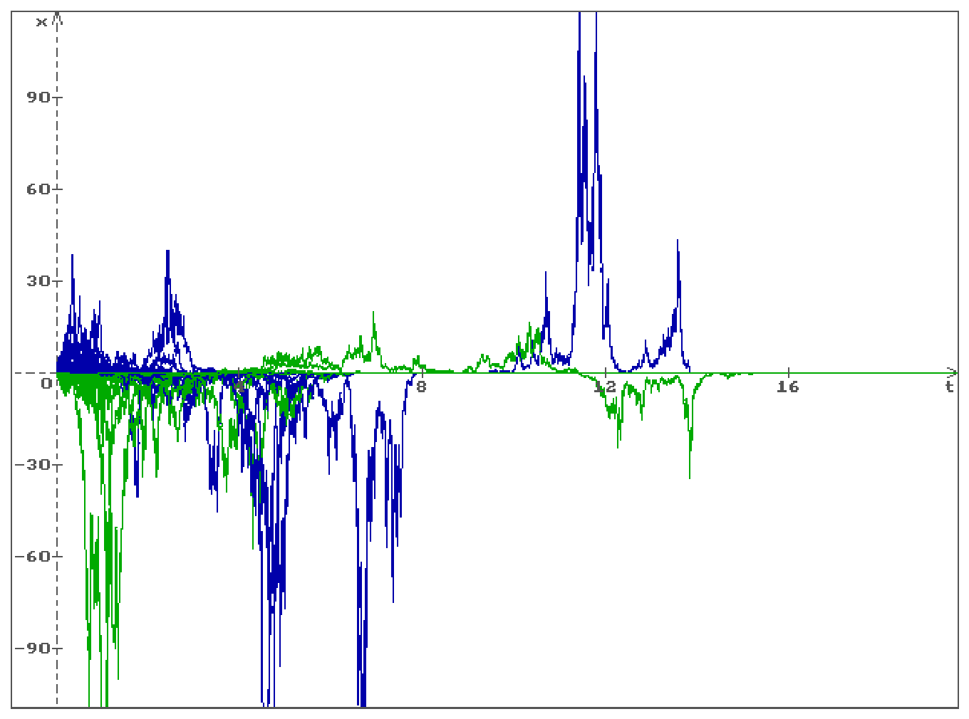
Let be $a_{11}=0.6$, $a_{12}=0.2$, $a_{21}=-0.2$, $a_{22}=0.4$, ${\sigma }_1=5$, ${\sigma }_2=4$, $x_1\left(0\right)=2$, $x_2\left(0\right)=-1$. In this case, both equations of the system (11) are dependent on each other; the solutions of the first (blue) and the second (green) equations have positive and negative values (see Figure 4). The zero solution is stable in probability, so all trajectories converge to zero.

Remark 3.

Note that for the numerical simulation of trajectories of the Wiener processes in Examples 1–4, a special procedure is used, which in detail is described in [13], pp. 29–31.

5. Conclusions

The effect of stabilization by noise, obtained by R.Z. Khasminskii for a scalar linear stochastic differential equation, is generalized for a system of n linear stochastic differential equations. In comparison with the list of works provided in the introduction, devoted to the problems of stabilization via noise, the result obtained here is a new one. It is detailed and illustrated in the example of the system of two linear stochastic differential equations and can be naturally used for a system of linear differential equations of dimension $n>2$ in various applications.

References

1. Khasminskii, R.Z. Stochastic Stability of Differential Equations; Springer: Berlin/Heidelberg, Germany, 2012. [Google Scholar]
2. Gikhman, I.I.; Skorokhod, A.V. Stochastic Differential Equations; Springer: Berlin/Heidelberg, Germany, 1972. [Google Scholar]
3. Arnold, L. Stabilization by noise revisited. Zamm-J. Appl. Math. Mech. Angew. Math. Mech. 1990, 70, 235–246. [Google Scholar] [CrossRef] [Scilit]
4. Deng, H.; Krstic, M. Output-feedback stabilization of stochastic nonlinear systems driven by noise of unknown covariance. Syst. Control Lett. 2000, 39, 173–182. [Google Scholar] [CrossRef] [Scilit]
5. Deng, H.; Krstic, M.; Williams, R.J. Stabilization of stochastic nonlinear systems driven by noise of unknown covariance. IEEE Trans. Autom. Control 2001, 46, 1237–1253. [Google Scholar] [CrossRef] [Scilit]
6. Jiang, Z.P.; Repperger, D. New results in decentralized adaptive nonlinear stabilization using output feedback. Int. J. Control 2001, 34, 659–673. [Google Scholar] [CrossRef] [Scilit]
7. Liu, S.-J.; Zhang, J.-F.; Jiang, Z.-P. Decentralized adaptive output-feedback stabilization for large-scale stochastic nonlinear systems. Automatica 2007, 43, 238–251. [Google Scholar] [CrossRef] [Scilit]
8. Hoshino, K.; Nishimura, Y.; Yamashita, Y.; Tsubakino, D. Global asymptotic stabilization of nonlinear deterministic systems using Wiener processes. IEEE Trans. Autom. Control 2016, 61, 2318–2323. [Google Scholar] [CrossRef] [Scilit]
9. Hoshino, K.; Nishimura, Y. Stabilization by noise for nonlinear systems with quantitative stability performances. IFAC-Pap. Online 2025, 59, 216–220. [Google Scholar] [CrossRef] [Scilit]
10. Shaikhet, L. About an unsolved problem of stabilization by noise for difference equations. Mathematics 2024, 12, 110. [Google Scholar] [CrossRef] [Scilit]
11. Shaikhet, L. About stabilization by Poisson’s jumps for stochastic differential equations. Appl. Math. Lett. 2024, 153, 109068. [Google Scholar] [CrossRef] [Scilit]
12. Shaikhet, L. About stabilization of the controlled inverted pendulum under stochastic perturbations of the type of Poisson’s jumps. Axioms 2025, 14, 29. [Google Scholar] [CrossRef] [Scilit]
13. Shaikhet, L. Lyapunov Functionals and Stability of Stochastic Functional Differential Equations; Springer Science & Business Media: Berlin/Heidelberg, Germany, 2013. [Google Scholar]
Figure 1. Fifty trajectories, x 1 ( t ) (blue) and x 2 ( t ) (green), of the solution of the system (11), a 11 = 0.5 , a 12 = 0 , a 21 = 0 , a 22 = 0.7 , σ 1 = 4 , σ 2 = 5 , x 1 ( 0 ) = 2 , x 2 ( 0 ) = 1 .
Axioms 15 00439 g001
Figure 2. Fifty trajectories, x 1 ( t ) (blue) and x 2 ( t ) (green), of the solution of the system (11), a 11 = 0.5 , a 12 = 0.25 , a 21 = 0 , a 22 = 0.5 , σ 1 = 4 , σ 2 = 4 , x 1 ( 0 ) = 2 , x 2 ( 0 ) = 1 .
Axioms 15 00439 g002
Figure 3. Fifty trajectories, x 1 ( t ) (blue) and x 2 ( t ) (green), of the solution of the system (11), a 11 = 0.5 , a 12 = 0 , a 21 = 0.25 , a 22 = 0.5 , σ 1 = 4 , σ 2 = 4 , x 1 ( 0 ) = 2 , x 2 ( 0 ) = 1 .
Axioms 15 00439 g003
Figure 4. Fifty trajectories, x 1 ( t ) (blue) and x 2 ( t ) (green), of the solution of the system (11), a 11 = 0.6 , a 12 = 0.2 , a 21 = 0.2 , a 22 = 0.4 , σ 1 = 5 , σ 2 = 4 , x 1 ( 0 ) = 2 , x 2 ( 0 ) = 1 .
Axioms 15 00439 g004
Disclaimer/Publisher’s Note: The statements, opinions and data contained in all publications are solely those of the individual author(s) and contributor(s) and not of MDPI and/or the editor(s). MDPI and/or the editor(s) disclaim responsibility for any injury to people or property resulting from any ideas, methods, instructions or products referred to in the content.