Controllability and Stability Analysis of Piecewise Dynamical Systems Under Integral Boundary Conditions

Abstract

This work investigates the controllability and stability properties of nonlinear piecewise dynamical systems subject to integral boundary conditions studied in arbitrary time domains. The study employs powerful mathematical ideas like fixed point theorems, Gramian-type matrices and the unified approach given by the theory of time scales. This unified approach provides results applicable seamlessly in various settings of continuous-time systems, discrete-time systems, and systems with hybrid behavior of both. This paper expands existing findings in the literature, providing a more complete view. To show the application of the theoretical results, a detailed example is presented and supported by numerical simulations to confirm the efficiency of the proposed methods.

1. Introduction

The concept of controllability was introduced by Kalman in 1960, and since then, it has become one of the main cornerstones of control theory. Controllability enables researchers to determine if a system can be driven from an initial state to a desired one by adequate control inputs [1,2,3]. This seminal idea has been applied in various fields of engineering, biology and other sciences from the design of optimal filters to the analysis of biological networks and the safety of systems. The controllability of linear and nonlinear systems has been extensively studied through the years and an extensive collection of literature exists [4,5,6]. However, many real-world systems exhibit behavior not captured by traditional models, e.g., impulsive effects or switching between different modes of operation. Such hybrid behavior is common in fields such as neural networks, population dynamics and biotechnology, where systems typically evolve via both continuous and discrete processes [7,8].

Toward the end of the nineteenth century, Hilger (1988) presented the theory of time scales, which integrates discrete and continuous analysis into a unified framework. Typically, discrete and continuous dynamical systems are examined independently, necessitating distinct proofs for each instance using discrete or continuous analysis. A time scale is a non-empty closed subset of the real numbers $\mathbb{R}$. The results derived from time scales are applicable to continuous, discrete, and any non-uniform time domains, proving beneficial in the analysis of complex dynamical systems. Consequently, the examination of differential equations on time scales has garnered significant global interest, with numerous scientists identifying applications in economics, control systems, population dynamics, and heat transfer systems [9,10,11,12,13,14,15]. While these systems have been studied for their stability and existence of solutions, their controllability, especially on hybrid time domains, has rarely been explored. This gap is significant, as many natural and engineered systems, such as the life cycles of certain insects species or economic systems, require a unified approach that combines continuous and discrete dynamics. Time scales theory provides such a framework [16,17,18,19]; however its application to piecewise impulsive systems has not been thoroughly investigated.

Fractional differential equations have been examined in several research concerning integral boundary conditions. These challenges originated from several scientific domains, including heat conduction, chemical engineering, subterranean water flow, and population dynamics, among others. For further information about fractional differential equations with integral boundary conditions, we direct the reader to [20] and the references therein.

In [21], the authors considered controllability, stability and existence of solutions for a class of piecewise impulsive dynamical systems defined on arbitrary time domains. After examining the current literature and according to their contributions, we observed that, up to now, there are no studies of nonlinear piecewise dynamical systems with integral boundary conditions in the framework of arbitrary time domains. It is this research gap that explains our study. In this work, we study the existence of solutions for a nonlinear dynamic system with impulses and integral boundary conditions. We also investigate the stability of these solutions under various conditions. Our analysis is performed on an arbitrary time domain.

$$\left\{\begin{array}{c}{z}^{\Delta }\left(\mathfrak{t}\right)={\mathcal{A}}_{\mu }\left(\mathfrak{t}\right)z\left(\mathfrak{t}\right)+{\mathcal{F}}_{\mu }(\mathfrak{t},z\left(\mathfrak{t}\right))+{\int }_{{\mathfrak{t}}_{\mu -1}}^{\mathfrak{t}}\mathcal{K}(\mathfrak{t},\hslash ){\mathcal{H}}_{\mu }(\hslash ,z(\hslash ))\Delta \hslash ,\mathfrak{t}\in {({\mathfrak{t}}_{\mu -1},{\mathfrak{t}}_{\mu }]}_T,\mu =1,2,\dots ,\ell ,\hfill \\ z\left({\mathfrak{t}}_{\mu }^{+}\right)-z\left({\mathfrak{t}}_{\mu }^{-}\right)=G_{\mu }({\mathfrak{t}}_{\mu },z\left({\mathfrak{t}}_{\mu }^{-}\right)),\mathfrak{t}={\mathfrak{t}}_{\mu },\hfill \\ z\left({\mathfrak{t}}_0\right)={\int }_0^{\xi }{\displaystyle \frac{{(\xi -\eta )}^{\nu -1}}{\Gamma \left(\nu \right)}}\delta (\eta ,z\left(\eta \right))d\eta .\hfill \end{array}\right.$$

(1)

Moreover, the study focuses on determining the controllability conditions for the subsequent system:

$$\left\{\begin{array}{c}{z}^{\Delta }\left(\mathfrak{t}\right)={\mathcal{A}}_{\mu }\left(\mathfrak{t}\right)z\left(\mathfrak{t}\right)+{\mathcal{B}}_{\mu }\left(\mathfrak{t}\right)u\left(\mathfrak{t}\right)+{\mathcal{F}}_{\mu }(\mathfrak{t},z\left(\mathfrak{t}\right))+{\int }_{{\mathfrak{t}}_{\mu -1}}^{\mathfrak{t}}\mathcal{K}(\mathfrak{t},\hslash ){\mathcal{H}}_{\mu }(\hslash ,z(\hslash ))\Delta \hslash ,\mathfrak{t}\in {({\mathfrak{t}}_{\mu -1},{\mathfrak{t}}_{\mu }]}_T,\mu =1,2,\dots ,\ell ,\hfill \\ z\left({\mathfrak{t}}_{\mu }^{+}\right)-z\left({\mathfrak{t}}_{\mu }^{-}\right)=G_{\mu }({\mathfrak{t}}_{\mu },z\left({\mathfrak{t}}_{\mu }^{-}\right)),\mathfrak{t}={\mathfrak{t}}_{\mu },\hfill \\ z\left({\mathfrak{t}}_0\right)={\int }_0^{\xi }{\displaystyle \frac{{(\xi -\eta )}^{\nu -1}}{\Gamma \left(\nu \right)}}\delta (\eta ,z\left(\eta \right))\Delta \eta .\hfill \end{array}\right.$$

(2)

In this setting, $z\left(\mathfrak{t}\right)\in {\mathbb{R}}^n$ denotes the state of the system at time $\mathfrak{t}$, while $u\left(\mathfrak{t}\right)\in {\mathbb{R}}^m$ represents the control input applied to the system. Let $I={[0,T]}_{\mathbb{T}}$, and let $0={\mathfrak{t}}_0<{\mathfrak{t}}_1<\cdots <{\mathfrak{t}}_{\ell }=T$ be a finite sequence of impulsive instants. For each $\mu =1,2,\dots ,\ell$, the system is considered on the interval ${({\mathfrak{t}}_{\mu -1},{\mathfrak{t}}_{\mu }]}_{\mathbb{T}}$. The right-hand and left-hand limits of z at $\mathfrak{t}={\mathfrak{t}}_{\mu }$ are respectively defined by $z\left({\mathfrak{t}}_{\mu }^{+}\right)={lim}_{h\to 0^{+}}z({\mathfrak{t}}_{\mu }+h),z\left({\mathfrak{t}}_{\mu }^{-}\right)={lim}_{h\to 0^{+}}z({\mathfrak{t}}_{\mu }-h).$ The coefficient matrix ${\mathcal{A}}_{\mu }\left(\mathfrak{t}\right)\in C_{\mathrm{rd}}\mathcal{R}(I,{\mathbb{R}}^{n\times n})$ is assumed to be rd-continuous and regressive, whereas ${\mathcal{B}}_{\mu }\left(\mathfrak{t}\right)\in C_{\mathrm{rd}}(I,{\mathbb{R}}^{n\times m})$ is assumed to be rd-continuous. The nonlinear functions ${\mathcal{F}}_{\mu }$, $\mathcal{K}$, ${\mathcal{H}}_{\mu }$, and $G_{\mu }$, with $G_{\ell }=0$, are assumed to satisfy appropriate hypotheses that will be specified later. For notational convenience, the state-transition matrix ${\varphi }_{{\mathcal{A}}_{\mu }}(\mathfrak{t},s)$ will be denoted by ${\varphi }_{\mu }(\mathfrak{t},s)$. To establish the existence of solutions to system (1), we first examine an associated piecewise impulsive system. This auxiliary analysis provides the analytical foundation for the subsequent development of the controllability results.

$$\left\{\begin{array}{cc}\hfill z^{\Delta }\left(\mathfrak{t}\right)& ={\mathcal{A}}_{\mu }\left(\mathfrak{t}\right)z\left(\mathfrak{t}\right)+{\mathcal{G}}_{\mu }\left(\mathfrak{t}\right),\mathfrak{t}\in {({\mathfrak{t}}_{\mu -1},{\mathfrak{t}}_{\mu }]}_{\mathbb{T}},\mu =1,2,\dots ,\ell ,\hfill \\ \hfill z\left({\mathfrak{t}}_{\mu }^{+}\right)& -z\left({\mathfrak{t}}_{\mu }^{-}\right)=G_{\mu }\left({\mathfrak{t}}_{\mu },z\left({\mathfrak{t}}_{\mu }^{-}\right)\right),\mathfrak{t}={\mathfrak{t}}_{\mu },\hfill \\ \hfill z\left({\mathfrak{t}}_0\right)& ={\int }_0^{\xi }{\displaystyle \frac{{(\xi -\eta )}^{\nu -1}}{\Gamma \left(\nu \right)}}\delta \left(\eta ,z\left(\eta \right)\right)\Delta \eta .\hfill \end{array}\right.$$

(3)

Here, ${\mathcal{G}}_{\mu }\left(\mathfrak{t}\right)\in C_{\mathrm{rd}}(I,{\mathbb{R}}^n)$ denotes a given rd-continuous vector-valued function, while all remaining symbols have the same meanings as those introduced for system (1).

The present work unifies and extends existing results within a time-scale framework, thereby allowing continuous, discrete, and hybrid dynamical systems to be treated in a single setting. To illustrate the practical relevance of the proposed theory, examples are provided on different time domains, demonstrating the applicability of the derived results across a range of dynamical behaviours. In addressing these issues, this study contributes to the analysis and control of complex dynamic systems and provides a rigorous foundation for the development of effective control strategies.

2. Preliminaries

The basic definitions and the results from the existing literature will be recalled in this section.

In the framework of dynamic equations, a time scale $\mathbb{T}$ is any non-empty closed subset of $\mathbb{R}$, carrying the topology and order of the real line. Examples include $\mathbb{R}$, $\mathbb{Z}$, and $\mathbb{N}$. Two key operators are defined:

1.

$\sigma :\mathbb{T}\to \mathbb{T},\sigma \left(\mathfrak{t}\right)=inf\{s\in \mathbb{T}:s>\mathfrak{t}\}$, where $inf\varnothing =sup\mathbb{T}$.

2.

$\delta :\mathbb{T}\to \mathbb{T},\delta \left(\mathfrak{t}\right)=sup\{s\in \mathbb{T}:s<\mathfrak{t}\}$, where $sup\varnothing =inf\mathbb{T}$.

These operators help analyze dynamic systems on both continuous and discrete time scales.

Define $\vartheta \left(t\right)=\sigma \left(t\right)-t$, with $\vartheta :\mathbb{T}\to [0,\infty )$, where $\sigma$ is the forward jump operator. We take ${\mathbb{T}}^{\kappa }$ to be the time scale $\mathbb{T}$, excluding the maximum element m if it is left-scattered; if such an element does not exist, ${\mathbb{T}}^{\kappa }$ is simply $\mathbb{T}$ [21]. This set ${\mathbb{T}}^{\kappa }$ is used to simplify analysis by excluding isolated maximum points when necessary.

Now we define the generalized derivative of the time scales.

Definition 1

([22]). Let $f:\mathbb{T}\to \mathbb{R}$ and suppose $t\in {\mathbb{T}}^{\kappa }$. A real number $f^{\delta }\left(t\right)$ is defined as the higher derivative of f at t; given any λ > 0, one can find a neighborhood U around t for which all s ∈ U fulfill

$$\left|{\displaystyle \frac{f\left(\sigma \right(t\left)\right)-f\left(s\right)}{\sigma \left(t\right)-s}}-f^{\delta }\left(t\right)\right|\le \lambda .$$

Remark 1.

The definition of the higher derivative $f^{\delta }\left(t\right)$ generalizes the concept of differentiation to arbitrary time scales. For specific choices of $\mathbb{T}$, it recovers familiar forms:

• When $\mathbb{T}=\mathbb{R}$, the higher derivative $f^{\delta }\left(t\right)$ coincides with the ordinary derivative of f; that is, $f^{\delta }\left(t\right)=f^{\prime }\left(t\right)$.
• When $\mathbb{T}=h\mathbb{Z}$ for some $h>0$, the higher derivative $f^{\delta }\left(t\right)$ reduces to the forward h-difference operator.

Now, we will explore the concept of the generalized exponential function.

Definition 2

([22]). If a function $p:T\to \mathbb{R}$ satisfies $1+\mu \left(t\right)p\left(t\right)\ne 0$ for all $t\in T$, then p is called regressive. The set of all such functions is represented by $\mathcal{R}$.

Definition 3

([22]). For any function p belonging to the set of regressive functions $\mathcal{R}$ and for any point $\mathfrak{t}$ in the time scale $\mathfrak{t}$, the circle minus operation, written as $\ominus p\left(\mathfrak{t}\right)$, is given by

$$\ominus p\left(\mathfrak{t}\right)=-{\displaystyle \frac{p\left(\mathfrak{t}\right)}{1+\mu \left(\mathfrak{t}\right)p\left(\mathfrak{t}\right)}}.$$

Definition 4

([22]). Given a regressive function $p\in \mathcal{R}$ and points $t,s\in T$, the function $e_p(t,s)$ defines the generalized exponential on the time scale $\mathfrak{t}$ as:

$$e_p(\mathfrak{t},s)=exp\left({\int }_s^t{\hslash }_{\mu \left(\tau \right)}\left(p\left(\tau \right)\right)\Delta \tau \right),$$

where ${\hslash }_h\left(z\right)$ is a function defined as:

$${\hslash }_h\left(z\right)=\left\{\begin{array}{cc}{\displaystyle \frac{1}{h}}log(1+zh),\hfill & \mathit{if}h>0,\hfill \\ z,\hfill & \mathit{if}h=0.\hfill \end{array}\right.$$

Here, $\mu \left(\tau \right)$ represents the graininess of the time scale $\mathfrak{t}$ at the point τ, and $\Delta \tau$ denotes the delta integral. This definition generalizes the classical exponential function to time scales by incorporating the structure of $\mathfrak{t}$ through the function ${\hslash }_h\left(z\right)$.

For further details and related concepts on time scales, readers are encouraged to refer to the relevant monographs [22,23].

Theorem 1

([24,25]). Let $A_0\in C_{rd}\mathcal{R}(T,M_n\left(\mathbb{R}\right))$. Then, the linear system below has a unique solution.

$$\left\{\begin{array}{cc}{z}^{\Delta }\left(\mathfrak{t}\right)=\hfill & A_0\left(\mathfrak{t}\right)z\left(\mathfrak{t}\right),\hfill \\ z\left({\mathfrak{t}}_0\right)=\hfill & {\int }_0^{\xi }{\displaystyle \frac{{(\xi -\eta )}^{\nu -1}}{\Gamma \left(\nu \right)}}\delta (\eta ,z\left(\eta \right))\Delta \eta \in {\Re }^n,{\mathfrak{t}}_0(\mathfrak{t}>{\mathfrak{t}}_0)\in T,\hfill \end{array}\right.$$

(4)

is written as $z\left(\mathfrak{t}\right)={\varphi }_{A_0}(\mathfrak{t},{\mathfrak{t}}_0){\int }_0^{\xi }{\displaystyle \frac{{(\xi -\eta )}^{\nu -1}}{\Gamma \left(\nu \right)}}\delta (\eta ,z\left(\eta \right))\Delta \eta$, where ${\varphi }_{A_0}(\mathfrak{t},{\mathfrak{t}}_0)$ is the matrix that describes the transitions of the system defined by Equation (4).

Theorem 2

([24]). If $A_0\in \mathrm{CrdR}(T,M_n\left(\mathbb{R}\right))$ and $G_0\in \mathrm{Crd}(T,{\mathbb{R}}^n)$, the following system has exactly one solution:

$$\left\{\begin{array}{c}{z}^{\Delta }\left(t\right)=A_0\left(t\right)z\left(t\right)+G_0\left(t\right),\hfill \\ z\left(t_0\right)={\int }_{{\xi }_0}^{\infty }{(\xi -\eta )}^{\nu -1}{\Gamma }_{\nu }\delta (\eta ,z\left(\eta \right))\Delta \eta \in {\mathbb{R}}^n,t_0,t>t_0\in T.\hfill \end{array}\right.$$

The solution is given by:

$$z\left(t\right)={\phi }_{A_0}(t,t_0){\int }_{{\xi }_0}^{\infty }{(\xi -\eta )}^{\nu -1}{\Gamma }_{\nu }\delta (\eta ,z\left(\eta \right))\Delta \eta +{\int }_{t_0}^t{\phi }_{A_0}(t,\sigma (\hslash ))G_0(\hslash )\Delta \hslash .$$

Lemma 1.

A function $z\in PC(I,{\mathbb{R}}^n)$ is known as a solution of the system (3) if it satisfies $z\left({\mathfrak{t}}_0\right)={\int }_0^{\xi }{\displaystyle \frac{{(\xi -\eta )}^{\nu -1}}{\Gamma \left(\nu \right)}}\delta (\eta ,z\left(\eta \right))\Delta \eta$ and the following equation

$$z\left(\mathfrak{t}\right)=\left\{\begin{array}{c}{\psi }_1(\mathfrak{t},{\mathfrak{t}}_0){\int }_0^{\xi }{\displaystyle \frac{{(\xi -\eta )}^{\nu -1}}{\Gamma \left(\nu \right)}}\delta (\eta ,z\left(\eta \right))\Delta \eta +{\int }_{{\mathfrak{t}}_0}^{\mathfrak{t}}{\psi }_1(t,\sigma (\hslash )){\mathcal{G}}_1(\hslash )\Delta \hslash ,\mathfrak{t}\in {({\mathfrak{t}}_0,{\mathfrak{t}}_1)}_T\hfill \\ {\psi }_{\mu }(\mathfrak{t},{\mathfrak{t}}_{\mu -1})\Delta (\mu -1;1){\int }_0^{\xi }{\displaystyle \frac{{(\xi -\eta )}^{\nu -1}}{\Gamma \left(\nu \right)}}\delta (\eta ,z\left(\eta \right))\Delta \eta \hfill \\ +{\displaystyle {\sum }_{i=1}^{\mu -1}}{\int }_{{\mathfrak{t}}_{i-1}}^{t_i}\Delta (\mu -1;i+1){\psi }_i(\mathfrak{t},\sigma (\hslash )){\mathcal{G}}_i(\hslash )\Delta \hslash ,\hfill \\ +{\displaystyle {\sum }_{i=1}^{\mu -1}}\Delta (\mu -1;i+1)G_i({\mathfrak{t}}_i,z\left({\mathfrak{t}}_i^{-}\right))\hfill \\ +{\int }_{{\mathfrak{t}}_{\mu -1}}^{\mathfrak{t}}{\psi }_{\mu }(t,\sigma (\hslash )){\mathcal{G}}_{\mu }(\hslash )\Delta \hslash ,\mathfrak{t}\in {({\mathfrak{t}}_{\mu -1},{\mathfrak{t}}_{\mu }]}_T,\mu =2,3,\dots \ell ,\hfill \end{array}\right.$$

(5)

where

$$\begin{array}{c}\hfill \Delta (\mu ,i)={\Pi }_{x=\mu }^i{\psi }_x(t_x,t_{x-1}).\end{array}$$

Proof. 

From Theorem 2, for all $\mathfrak{t}\in (t_0,t_1)$ we have

$$\begin{array}{c}\hfill z\left(\mathfrak{t}\right)={\psi }_1(\mathfrak{t},{\mathfrak{t}}_0){\int }_0^{\xi }{\displaystyle \frac{{(\xi -\eta )}^{\nu -1}}{\Gamma \left(\nu \right)}}\delta (\eta ,z\left(\eta \right))\Delta \eta +{\int }_{{\mathfrak{t}}_0}^{\mathfrak{t}}{\psi }_1(t,\sigma (\hslash )){\mathcal{G}}_1(\hslash )\Delta \hslash ,\end{array}$$

which gives

$$\begin{array}{c}\hfill z\left({\mathfrak{t}}_1\right)={\psi }_1(t_1,t_0){\int }_0^{\xi }{\displaystyle \frac{{(\xi -\eta )}^{\nu -1}}{\Gamma \left(\nu \right)}}\delta (\eta ,z\left(\eta \right))\Delta \eta +{\int }_{{\mathfrak{t}}_0}^{t_1}{\psi }_1(t,\sigma (\hslash )){\mathcal{G}}_1(\hslash )\Delta ,\hslash ,\end{array}$$

also for $\mathfrak{t}\in {(t_1,t_2]}_T$

$$\begin{array}{cc}\hfill z\left(\mathfrak{t}\right)=& {\psi }_1(t,t_1)z\left({\mathfrak{t}}_1^{+}\right)+{\int }_{{\mathfrak{t}}_1}^{\mathfrak{t}}{\psi }_2(t,\sigma (\hslash )){\mathcal{G}}_2(\hslash )\Delta \hslash ,\hfill \\ \hfill z\left(\mathfrak{t}\right)=& {\psi }_1(t,t_1)\left\{{\psi }_1(t_1,t_0){\int }_0^{\xi }{\displaystyle \frac{{(\xi -\eta )}^{\nu -1}}{\Gamma \left(\nu \right)}}\delta (\eta ,z\left(\eta \right))\Delta \eta +{\int }_{{\mathfrak{t}}_0}^{\mathfrak{t}}{\psi }_1(t,\sigma (\hslash )){\mathcal{G}}_1(\hslash )\Delta \hslash \right\}\hfill \\ \hfill & +G_1(t_1,z\left({\mathfrak{t}}_1^{+}\right))+{\int }_{{\mathfrak{t}}_1}^{\mathfrak{t}}{\psi }_2(t,\sigma (\hslash )){\mathcal{G}}_2(\hslash )\Delta \hslash .\hfill \end{array}$$

When $\mu =2$, the solution $z\left(\mathfrak{t}\right)$ has the form given in Equation (5). Now, the result holds for a fixed $\mu =l$, where $3\le l\le \ell -1$; that is, $z\left(\mathfrak{t}\right)$ can be expressed in the same form:

$$\begin{array}{cc}\hfill z\left(\mathfrak{t}\right)=& {\psi }_l(t,t_{l-1})\{\Delta (l-1;1){\int }_0^{\xi }{\displaystyle \frac{{(\xi -\eta )}^{\nu -1}}{\Gamma \left(\nu \right)}}\delta (\eta ,z\left(\eta \right))\Delta \eta \hfill \\ \hfill & +{\displaystyle \sum _{i=1}^{l-1}}{\int }_{{\mathfrak{t}}_{i-1}}^{t_i}\Delta (l-1;i+1){\psi }_i(\mathfrak{t},\sigma (\hslash )){\mathcal{G}}_i(\hslash )\Delta \hslash \hfill \\ \hfill & +{\displaystyle \sum _{i=1}^{l-1}}\Delta (l-1;i+1)G_i({\mathfrak{t}}_i,z\left({\mathfrak{t}}_i^{-}\right))\}\hfill \\ \hfill & +{\int }_{{\mathfrak{t}}_{l-1}}^{\mathfrak{t}}{\psi }_l(t,\sigma (\hslash )){\mathcal{G}}_l(\hslash )\Delta \hslash ,\mathfrak{t}\in {(t_{l-1},t_l]}_T\hfill \end{array}$$

Thus, we have

$$\begin{array}{cc}\hfill z\left({\mathfrak{t}}_l\right)=& {\psi }_l(t_l,t_{l-1})\{\Delta (l-1;1){\int }_0^{\xi }{\displaystyle \frac{{(\xi -\eta )}^{\nu -1}}{\Gamma \left(\nu \right)}}\delta (\eta ,z\left(\eta \right))\Delta \eta \hfill \\ \hfill & +{\displaystyle \sum _{i=1}^{l-1}}{\int }_{{\mathfrak{t}}_{i-1}}^{t_i}\Delta (l-1;i+1){\psi }_i(\mathfrak{t},\sigma (\hslash )){\mathcal{G}}_i(\hslash )\Delta \hslash \hfill \\ \hfill & +{\displaystyle \sum _{i=1}^{l-1}}\Delta (l-1;i+1)G_i({\mathfrak{t}}_i,z\left({\mathfrak{t}}_i^{-}\right))\}+{\int }_{{\mathfrak{t}}_{l-1}}^{t_l}{\psi }_l(t_l,\sigma (\hslash )){\mathcal{G}}_l(\hslash )\Delta \hslash ,\hfill \end{array}$$

So, for all $\mathfrak{t}\in {(t_l,t_{l+1}]}_T$

$$\begin{array}{cc}\hfill z\left(\mathfrak{t}\right)=& {\psi }_{l+1}(t,t_l)\{\Delta (l;1){\int }_0^{\xi }{\displaystyle \frac{{(\xi -\eta )}^{\nu -1}}{\Gamma \left(\nu \right)}}\delta (\eta ,z\left(\eta \right))\Delta \eta +{\displaystyle \sum _{i=1}^l}{\int }_{{\mathfrak{t}}_{i-1}}^{t_i}\Delta (l;i+1){\psi }_i(\mathfrak{t},\sigma (\hslash )){\mathcal{G}}_i(\hslash )\Delta \hslash \hfill \\ \hfill & +{\displaystyle \sum _{i=1}^l}\Delta (l;i+1)G_i({\mathfrak{t}}_i,z\left({\mathfrak{t}}_i^{-}\right))\}+{\int }_{{\mathfrak{t}}_l}^{\mathfrak{t}}{\psi }_{l+1}(t,\sigma (\hslash )){\mathcal{G}}_{l+1}(\hslash )\Delta \hslash \hfill \end{array}$$

This demonstrates that the result is true for $\mu =l+1$. By the principle of Mathematical Induction, the form of the solution $z\left(\mathfrak{t}\right)$ given by Equation (5) holds for all $\mu$ in the range $2\le \mu \le \ell$.

□

In light of the above lemma we introduce the following definition.

Definition 5.

A function $z\in PC(I,{\mathbb{R}}^n)$ is known as solution of the system (1) if it holds $z\left({\mathfrak{t}}_0\right)={\int }_0^{\xi }{\displaystyle \frac{{(\xi -\eta )}^{\nu -1}}{\Gamma \left(\nu \right)}}\delta (\eta ,z\left(\eta \right))\Delta \eta$ and the following equation

$$z\left(\mathfrak{t}\right)=\left\{\begin{array}{c}{\psi }_1(\mathfrak{t},{\mathfrak{t}}_0){\int }_0^{\xi }{\displaystyle \frac{{(\xi -\eta )}^{\nu -1}}{\Gamma \left(\nu \right)}}\delta (\eta ,z\left(\eta \right))\Delta \eta +{\int }_{{\mathfrak{t}}_0}^{\mathfrak{t}}{\psi }_1(t,\sigma (\hslash ))\left({\mathcal{F}}_1\right(\hslash ,z(\hslash )\hfill \\ +{\int }_{{\mathfrak{t}}_0}^{\hslash }\mu (\hslash ,s){\mathcal{H}}_1(s,z\left(s\right))\Delta s)\Delta \hslash ,\mathfrak{t}\in {({\mathfrak{t}}_0,{\mathfrak{t}}_1)}_T\hfill \\ {\psi }_{\mu }(\mathfrak{t},{\mathfrak{t}}_{\mu -1})\{\Delta (\mu -1;1){\int }_0^{\xi }{\displaystyle \frac{{(\xi -\eta )}^{\nu -1}}{\Gamma \left(\nu \right)}}\delta (\eta ,z\left(\eta \right))\Delta \eta \hfill \\ +{\displaystyle {\sum }_{i=1}^{\mu -1}}{\int }_{{\mathfrak{t}}_{i-1}}^{t_i}\Delta (\mu -1;i+1){\psi }_i({\mathfrak{t}}_i,\sigma (\hslash ))({\mathcal{F}}_i(\hslash ,z(\hslash ))\hfill \\ +{\int }_{{\mathfrak{t}}_{i-1}}^{\hslash }\mu (\hslash ,z(\hslash )){\mathcal{H}}_i(s,z\left(s\right))\Delta s)\Delta \hslash ,+{\displaystyle {\sum }_{i=1}^{\mu -1}}\Delta (\mu -1;i+1)G_i({\mathfrak{t}}_i,z\left({\mathfrak{t}}_i^{-}\right))\}\hfill \\ +{\int }_{{\mathfrak{t}}_{\mu -1}}^{\mathfrak{t}}{\psi }_{\mu }(t,\sigma (\hslash ))({\mathcal{F}}_{\mu }(\hslash ,z(\hslash ))+{\int }_{{\mathfrak{t}}_{\mu -1}}^{\hslash }\mu (\hslash ,s){\mathcal{H}}_{\mu }(s,z\left(s\right))\Delta s)\Delta \hslash ,\mathfrak{t}\in {({\mathfrak{t}}_{\mu -1},{\mathfrak{t}}_{\mu }]}_T,\mu =2,3,\dots \ell .\hfill \end{array}\right.$$

Our main results are based on the following set of assumptions.

1.

The non-linear functions ${\mathcal{F}}_{\mu }$, ${\mathcal{H}}_{\mu }$, $G_{\mu }$: ${[{\mathfrak{t}}_{\mu -1},t_{\mu }]}_T\times {\Re }^n\to {\Re }^n$, $\mu =1,2,\dots ,\ell$ are continuous and there exist positive constants $L_{{\mathcal{F}}_{\mu }}$, $L_{{\mathcal{H}}_{\mu }}$, and $L_{G_{\mu }}$ such that

$$\begin{array}{c}\hfill \parallel {\mathcal{F}}_{\mu }(t,z)-{\mathcal{F}}_{\mu }(t,x)\parallel \le L_{{\mathcal{F}}_{\mu }}\parallel z-x\parallel \\ \hfill \parallel {\mathcal{H}}_{\mu }(t,z)-{\mathcal{H}}_{\mu }(t,x)\parallel \le L_{{\mathcal{H}}_{\mu }}\parallel z-x\parallel \\ \hfill \parallel G_{\mu }(t,z)-G_{\mu }(t,x)\parallel \le L_{G_{\mu }}\parallel z-x\parallel \end{array}$$

for all $\mathfrak{t}\in {[t\mu -1,t_{\mu }]}_T$ and $z,x\in {\Re }^n$.

2.

Let $\mathcal{K}$ be a continuous function on the domain ${[{\mathfrak{t}}_{\mu -1},t_{\mu }]}_T\times {[{\mathfrak{t}}_{\mu -1},t_{\mu }]}_T\to \mathbb{R}$, with $\mu =1,2,\dots ,\ell$, and suppose there exists $M_{\mathcal{K}}>0$ such that

$${\int }_{{\mathfrak{t}}_{\mu -1}}^{t_{\mu }}\left|\mathcal{K}(t,s)\right|\Delta s\le M_{\mathcal{K}}.$$

For the convincing of notation, we set

$$\begin{array}{cc}\hfill \parallel {\mathcal{F}}_{\mu }(t,0)\parallel \le & M_{{\mathcal{F}}_{\mu }},\parallel {\mathcal{H}}_{\mu }(t,0)\parallel \le M_{{\mathcal{H}}_{\mu }},\parallel G_{\mu }(t,0)\parallel \le M_{G_{\mu }},\mu =1,2,\dots ,\ell ;\hfill \\ \hfill \parallel {\psi }_{\mu }(\mathfrak{t},s)\parallel \le & M_{\mu },t,s\in {[{\mathfrak{t}}_{\mu -1},t_{\mu }]}_T,\mu =1,2,\dots ,\ell ;\hfill \\ \hfill a_{\mu }=& M_{{\mathcal{F}}_{\mu }}+M_{\mathcal{K}}{M}_{{\mathcal{H}}_{\mu }};b_{\mu }=L_{{\mathcal{F}}_{\mu }}+M_{\mathcal{K}}{L}_{{\mathcal{H}}_{\mu }},\mu =1,2,\dots ,\ell ;\hfill \\ \hfill {\mathbb{M}}_1=& M_1{l}_1{a}_1;{\mathbb{M}}_{\mu }=M_{\mu }{l}_{\mu }{b}_{\mu }+{\displaystyle \sum _{i=1}^{\mu -1}}{M}_{\mu }\parallel \Delta (\mu -1;i+1)\parallel (M_i{l}_i{a}_i+M_{{\mathbf{G}}_{\mathbf{i}}}),\mu =2,3,\dots ,\ell ;\hfill \\ \hfill {\mathbb{Z}}_1=& M_1{l}_1{b}_1;{\mathbb{Z}}_{\mu }=M_{\mu }{l}_{\mu }{b}_{\mu }+{\displaystyle \sum _{i=1}^{\mu -1}}{M}_{\mu }\parallel \Delta (\mu -1;i+1)\parallel (M_i{l}_i{b}_i+M_{{\mathbf{G}}_{\mathbf{i}}}),\mu =2,3,\dots ,\ell .\hfill \end{array}$$

3. Existence and Stability

This section aims to demonstrate the existence of solutions while providing a stability analysis of the system in Equation (1).

Theorem 3.

If assumptions (1) and (2) are satisfied, then Equation (1) admits a unique solution. Furthermore, this solution satisfies the condition:

$$\mathbb{Z}=\underset{\mu =1,2,\dots ,\ell }{max}\left\{{\mathbb{Z}}_{\mu }\right\}<1,$$

Proof. 

For a positive constant $\rho$ given as

$$\begin{array}{c}\hfill \rho \ge max\left\{\begin{array}{c}{\displaystyle \frac{M_1\parallel {\int }_0^{\xi }\frac{{(\xi -\eta )}^{\nu -1}}{\Gamma \left(\nu \right)}\delta (\eta ,z\left(\eta \right))\Delta \eta \parallel +{\mathbb{M}}_1}{1-{\mathbb{Z}}_1}},\hfill \\ ma{x}_{\mu =2,3,\dots ,\ell }{\displaystyle \frac{M_{\mu }\parallel \Delta (\mu -1;1){\int }_0^{\xi }\frac{{(\xi -\eta )}^{\nu -1}}{\Gamma \left(\nu \right)}\delta (\eta ,z\left(\eta \right))\Delta \eta \parallel +{\mathbb{M}}_{\mu }}{1-{\mathbb{Z}}_{\mu }}},\hfill \end{array}\right.\end{array}$$

define an operator $F:D_{\rho }\to D_{\rho }$ such that

$$\begin{array}{cc}\hfill (Fz)(\mathfrak{t})=& {\psi }_1(\mathfrak{t},{\mathfrak{t}}_0){\int }_0^{\xi }{\displaystyle \frac{{(\xi -\eta )}^{\nu -1}}{\Gamma (\nu )}}\delta (\eta ,z(\eta ))\Delta \eta +{\int }_{{\mathfrak{t}}_0}^{\mathfrak{t}}{\psi }_1(t,\sigma (\hslash ))({\mathcal{F}}_1(\hslash ,z(\hslash )\hfill \\ \hfill & +{\int }_{{\mathfrak{t}}_0}^{\hslash }\mu (\hslash ,s){\mathcal{H}}_1(s,z(s))\Delta s)\Delta \hslash ,\mathfrak{t}\in {({\mathfrak{t}}_0,{\mathfrak{t}}_1)}_T\hfill \\ \hfill & (\times )(Fz)(\mathfrak{t})={\psi }_{\mu }(\mathfrak{t},{\mathfrak{t}}_{\mu -1})\{\Delta (\mu -1;1){\int }_0^{\xi }{\displaystyle \frac{{(\xi -\eta )}^{\nu -1}}{\Gamma (\nu )}}\delta (\eta ,z(\eta ))\Delta \eta \hfill \\ \hfill & +{\displaystyle \sum _{i=1}^{\mu -1}}{\int }_{{\mathfrak{t}}_{i-1}}^{t_i}\Delta (\mu -1;i+1){\psi }_i({\mathfrak{t}}_i,\sigma (\hslash ))({\mathcal{F}}_i(\hslash ,z(\hslash ))\hfill \\ \hfill & +{\int }_{{\mathfrak{t}}_{i-1}}^{\hslash }\mu (\hslash ,z(\hslash )){\mathcal{H}}_1(s,z(s))\Delta s)\Delta \hslash ,+{\displaystyle \sum _{i=1}^{\mu -1}}\Delta (\mu -1;i+1)G_i({\mathfrak{t}}_i,z({\mathfrak{t}}_i^{-}))\}\hfill \\ \hfill & +{\int }_{{\mathfrak{t}}_{\mu -1}}^{\mathfrak{t}}{\psi }_{\mu }(t,\sigma (\hslash ))({\mathcal{F}}_{\mu }(\hslash ,z(\hslash ))+{\int }_{{\mathfrak{t}}_{\mu -1}}^{\hslash }\mu (\hslash ,s){\mathcal{H}}_{\mu }(s,z(s))\Delta s)\Delta \hslash ,\mathfrak{t}\in {({\mathfrak{t}}_{\mu -1},{\mathfrak{t}}_{\mu }]}_T,\mu =2,3,\dots \ell .\hfill \end{array}$$

Any function $z\in PC(I,{\mathbb{R}}^n)$ that fulfills $Fz=z$ serves as a FP of F and solves the system given by Equation (1). We use the Banach fixed point theorem (FPT) to prove the existence of such a function. For ease of understanding, the proof is divided into two main steps:

1.

We demonstrate that the operator F maps $D_{\rho }$ into itself. To this end, let $z\in D_{\rho }$ and $\mathfrak{t}\in {({\mathfrak{t}}_0,{\mathfrak{t}}_1)}_T$; we calculate

$$\begin{array}{cc}\hfill \parallel \left(Fz\right)\left(\mathfrak{t}\right)\parallel \le & ∥{\psi }_1(\mathfrak{t},{\mathfrak{t}}_0){\int }_0^{\xi }{\displaystyle \frac{{(\xi -\eta )}^{\nu -1}}{\Gamma \left(\nu \right)}}\delta (\eta ,z\left(\eta \right))\Delta \eta ∥\hfill \\ \hfill & +{\int }_{{\mathfrak{t}}_0}^{\mathfrak{t}}∥{\psi }_1(t,\sigma (\hslash ))∥∥{\mathcal{F}}_1(\hslash ,z(\hslash ))∥\hfill \\ \hfill & +{\int }_{{\mathfrak{t}}_0}^{\hslash }\left|\mathcal{K}(\hslash ,s)\right|∥{\mathcal{H}}_1(s,z\left(s\right))∥\Delta s)\Delta \hslash .\hfill \end{array}$$

Now, using the assumption (1) and (2), we get

$$\begin{array}{cc}\hfill ∥\left(Fz\right)\left(\mathfrak{t}\right)∥\le & M_1∥{\int }_0^{\xi }{\displaystyle \frac{{(\xi -\eta )}^{\nu -1}}{\Gamma \left(\nu \right)}}\delta (\eta ,z\left(\eta \right))\Delta \eta ∥M_1{l}_1(M_{{\mathcal{F}}_1}+M_{\mathcal{K}}{M}_{{\mathcal{H}}_1})\hfill \\ \hfill & +M_1{l}_1(L_{{\mathcal{F}}_1}+M_{\mathcal{K}}{L}_{{\mathcal{H}}_1})\rho \hfill \\ \hfill \le & M_1∥{\int }_0^{\xi }{\displaystyle \frac{{(\xi -\eta )}^{\nu -1}}{\Gamma \left(\nu \right)}}\delta (\eta ,z\left(\eta \right))\Delta \eta ∥+{\mathbb{M}}_1+{\mathbb{Z}}_1\rho \hfill \\ \hfill \le & \rho .\hfill \end{array}$$

(6)

For every $z\in D_{\rho }$ and $\mathfrak{t}\in {({\mathfrak{t}}_{\mu -1},{\mathfrak{t}}_{\mu }]}_T$ $\mu =2,3,\dots ,\ell$, we have

$$\begin{array}{cc}\hfill \left(Fz\right)\left(\mathfrak{t}\right)\le & M_{\mu }\parallel \Delta (\mu -1;1){\int }_0^{\xi }{\displaystyle \frac{{(\xi -\eta )}^{\nu -1}}{\Gamma \left(\nu \right)}}\delta (\eta ,z\left(\eta \right))\Delta \eta \parallel \hfill \\ \hfill & +{\displaystyle \sum _{i=1}^{\mu -1}}{M}_{\mu }\parallel \Delta (\mu -1;i+1)\parallel M_i{l}_i(L_{{\mathcal{F}}_i}\rho +M_{{\mathcal{F}}_i}+M_{\mathcal{K}}{L}_{{\mathcal{H}}_i}\rho +M_{\mathcal{K}}{M}_{{\mathcal{H}}_i})\hfill \\ \hfill & +{\displaystyle \sum _{i=1}^{\mu -1}}{M}_{\mu }\parallel \Delta (\mu -1;i+1)\parallel \parallel M_{G_i}\hfill \\ \hfill & +L{G}_i\parallel \rho +M_{\mu }{l}_{\mu }(L_{{\mathcal{F}}_{\mu }}\rho +M_{{\mathcal{F}}_{\mu }}+M_{\mathcal{K}}{L}_{{\mathcal{H}}_{\mu }}\rho +M_{\mathcal{K}}{M}_{{\mathcal{H}}_{\mu }})\hfill \\ \hfill \le & M_{\mu }\parallel \Delta (\mu -1;1){\int }_0^{\xi }{\displaystyle \frac{{(\xi -\eta )}^{\nu -1}}{\Gamma \left(\nu \right)}}\delta (\eta ,z\left(\eta \right))\Delta \eta \parallel +{\mathbb{M}}_{\mu }+{\mathbb{Z}}_{\mu }\rho \hfill \\ \hfill \le & \rho \hfill \end{array}$$

(7)

As a consequence of the previous two inequalities, we have for all $\mathfrak{t}\in I$, the norm of $Fz$ satisfies: $\parallel Fz\parallel \le \rho$. Therefore, the operator F maps the set $D_{\rho }$ into itself.

2.

We show that the operator F satisfies the contraction mapping property. We consider two arbitrary functions $z,x\in D_{\rho }$ and a point $\mathfrak{t}\in {({\mathfrak{t}}_0,{\mathfrak{t}}_1)}_T$, and we get

$$\begin{array}{cc}\hfill \parallel \left(Fz\right)\left(\mathfrak{t}\right)-\left(Fx\right)\left(\mathfrak{t}\right)\parallel \le & {\int }_{{\mathfrak{t}}_0}^{\mathfrak{t}}\parallel {\psi }_1(t,\sigma (\hslash ))\parallel (\parallel {\mathcal{F}}_1(\hslash ,z(\hslash ))-{\mathcal{F}}_1(\hslash ,x(\hslash ))\parallel \Delta \hslash \hfill \\ \hfill & +{\int }_{{\mathfrak{t}}_0}^{\mathfrak{t}}\parallel {\psi }_1(t,\sigma (\hslash ))\parallel {\int }_{{\mathfrak{t}}_0}^{\hslash }\left|\mathcal{K}(\hslash ,s)\right|\parallel {\mathcal{H}}_1(s,z\left(s\right))-{\mathcal{H}}_1(s,x\left(s\right))\parallel )\Delta s\Delta \hslash \hfill \\ \hfill \le & M_1{l}_1{L}_{{\mathcal{F}}_1}{\parallel z-x\parallel }_{PC}+M_1{l}_1{M}_{\mathcal{K}}{L}_{{\mathcal{H}}_1}{\parallel z-x\parallel }_{PC}\hfill \\ \hfill \le & {\mathbb{Z}}_1{\parallel z-x\parallel }_{PC}\hfill \end{array}$$

(8)

Also for $z,x\in D_{\rho }$ and $\mathfrak{t}\in {({\mathfrak{t}}_{\mu -1},t_{\mu }]}_T$, $\mu =2,3,\dots ,\ell$, we have

$$\parallel \left(Fz\right)\left(\mathfrak{t}\right)-\left(Fx\right)\left(\mathfrak{t}\right)\parallel \le {\mathbb{Z}}_{\mu }{\parallel z-x\parallel }_{PC}$$

(9)

From the Inequalities (8) and (9), we derive the following result

$${\parallel \left(Fz\right)-\left(Fx\right)\parallel }_{PC}\le \mathbb{Z}{\parallel z-x\parallel }_{PC},$$

we conclude that the operator F is a contraction mapping.

With Steps 1 and 2, we confirm that F meets all prerequisites of the Banach FPT, which secures the existence and uniqueness of a solution to Equation (1). □

Under less restrictive conditions, we aim to demonstrate the existence of at least one solution to Equation (1), using Schauder’s FPT as the central tool. The involved nonlinear mappings ${\mathcal{F}}_{\mu },{\mathcal{H}}_{\mu },G_{\mu }$ are assumed to be continuous on their domains, with uniform bounds provided by positive constants $C_{{\mathcal{F}}_{\mu }},C_{{\mathcal{H}}_{\mu }},C_{G_{\mu }}$.

We set

$$\begin{array}{cc}\hfill & d_{\mu }=C_{{\mathcal{F}}_{\mu }}+M_{\mathcal{K}}{C}_{{\mathcal{H}}_{\mu }},\mu =1,2,\dots ,\ell ;{\mathcal{M}}_1=M_1{l}_1{d}_1;\hfill \\ \hfill & {\mathcal{M}}_{\mu }=M_{\mu }{l}_{\mu }{d}_{\mu }+{\displaystyle \sum _{i=1}^{\mu -1}}{M}_{\mu }\parallel \Delta (\mu -1;i+1)\parallel (M_i{l}_i{d}_i+C_{G_i}),\mu =2,3,\dots ,\ell .\hfill \end{array}$$

Theorem 4.

If assumptions (2) and (3) hold, then the system described by Equation (1) admits at least one solution.

Proof. 

We define $F:D_{{\rho }_1}\to D_{{\rho }_1}$ in the same way as in Theorem 3

$$\begin{array}{c}\hfill {\rho }_1\ge max\left\{\begin{array}{c}{M}_1\parallel {\int }_0^{\xi }{\displaystyle \frac{{(\xi -\eta )}^{\nu -1}}{\Gamma \left(\nu \right)}}\delta (\eta ,z\left(\eta \right))\Delta \eta \parallel +{\mathcal{M}}_1,\hfill \\ ma{x}_{\mu =2,3,\dots ,\ell }\left(M_{\mu }\parallel \Delta (\mu -1;1){\int }_0^{\xi }{\displaystyle \frac{{(\xi -\eta )}^{\nu -1}}{\Gamma \left(\nu \right)}}\delta (\eta ,z\left(\eta \right))\Delta \eta \parallel +{\mathcal{M}}_{\mu }\right)\hfill \end{array}\right..\end{array}$$

Applying the same method as in step 1 of Theorem 3, we verify that the operator F preserves the set $D_{{\rho }_1}$ under the conditions given by assumptions (2) and (3). Specifically, for all $z\in D_{{\rho }_1}$ and $\mathfrak{t}\in I$, we have: ${\parallel Fz\parallel }_{PC}\le {\rho }_1$.

Step 2: To prove that F is a continuous operator, let ${\left\{z_n\right\}}_{n=1}^{\infty }$ be any sequence in $D_{{\rho }_1}$ that satisfies the following condition: $\parallel z_n{-z\parallel }_{PC}\to 0\mathrm{as}n\to \infty$, where $z\in D_{{\rho }_1}$. Our goal is to show that: $\parallel F{z}_n{-Fz\parallel }_{PC}\to 0\mathrm{as}n\to \infty$. For any $\mathfrak{t}\in {({\mathfrak{t}}_0,{\mathfrak{t}}_1)}_T$

$$\begin{array}{cc}\hfill \parallel \left(F{z}_n\right)\left(\mathfrak{t}\right)-\left(Fz\right)\left(\mathfrak{t}\right)\parallel \le & {\int }_{{\mathfrak{t}}_0}^{\mathfrak{t}}\parallel {\psi }_1(t,\sigma (\hslash ))\parallel \parallel {\mathcal{F}}_1(\hslash ,z_n(\hslash ))-{\mathcal{F}}_1(\hslash ,z(\hslash ))\parallel \Delta \hslash \hfill \\ \hfill & +{\int }_{{\mathfrak{t}}_0}^{\mathfrak{t}}\parallel {\psi }_1(t,\sigma (\hslash ))\parallel {\int }_{{\mathfrak{t}}_0}^{\hslash }\left|\mathcal{K}(\hslash ,s)\right|\parallel {\mathcal{H}}_1(s,z_n\left(s\right))-{\mathcal{H}}_1(s,z\left(s\right))\parallel )\Delta s\Delta \hslash \hfill \\ \hfill \le & M_1{\int }_{{\mathfrak{t}}_0}^{\mathfrak{t}}\parallel {\mathcal{F}}_1(\hslash ,z(\hslash ))-{\mathcal{F}}_1(\hslash ,x(\hslash ))\parallel \Delta \hslash \hfill \\ \hfill & +M_1{\int }_{{\mathfrak{t}}_0}^{\mathfrak{t}}{\int }_{{\mathfrak{t}}_0}^{\hslash }\left|\mathcal{K}(\hslash ,s)\right|\parallel {\mathcal{H}}_1(s,z\left(s\right))-{\mathcal{H}}_1(s,x\left(s\right))\parallel )\Delta s\Delta \hslash .\hfill \end{array}$$

(10)

Also, for $\mathfrak{t}\in {({\mathfrak{t}}_{\mu -1},t_{\mu }]}_T$, $\mu =2,3,\dots ,\ell$,

$$\begin{array}{cc}\hfill \parallel \left(F{z}_n\right)\left(\mathfrak{t}\right)-\left(Fz\right)\left(\mathfrak{t}\right)\parallel \le & {\displaystyle \sum _{i=1}^{\mu -1}}{\int }_{{\mathfrak{t}}_{i-1}}^{t_i}{M}_{\mu }\parallel \Delta (\mu -1;i+1)\parallel M_i(\parallel {\mathcal{F}}_i(\hslash ,z_n(\hslash ))-{\mathcal{F}}_i(\hslash ,z(\hslash ))\parallel \hfill \\ \hfill & +{\int }_{{\mathfrak{t}}_{i-1}}^{\hslash }\left|\mathcal{K}(\hslash ,s)\right|\parallel {\mathcal{H}}_i(s,z_n\left(s\right))-{\mathcal{H}}_i(s,z\left(s\right))\parallel \Delta s)\Delta \hslash ,\hfill \\ \hfill & +{\displaystyle \sum _{i=1}^{\mu -1}}{M}_{\mu }\parallel \Delta (\mu -1;i+1)\parallel \parallel G_i({\mathfrak{t}}_i,z_n\left(t_i^{-}\right))-G_i({\mathfrak{t}}_i,z\left({\mathfrak{t}}_i^{-}\right))\parallel \hfill \\ \hfill & +{\int }_{{\mathfrak{t}}_{\mu -1}}^{\mathfrak{t}}{M}_{\mu }(\parallel {\mathcal{F}}_{\mu }(\hslash ,z_n(\hslash ))-{\mathcal{F}}_{\mu }(\hslash ,z(\hslash ))\parallel \hfill \\ \hfill & +{\int }_{{\mathfrak{t}}_{\mu -1}}^{\hslash }\left|\mathcal{K}(\hslash ,s)\right|\parallel {\mathcal{H}}_{\mu }(s,z_n\left(s\right))-{\mathcal{H}}_{\mu }(s,z\left(s\right))\parallel \Delta s)\Delta \hslash .\hfill \end{array}$$

(11)

Because ${\mathcal{F}}_{\mu }$, ${\mathcal{H}}_{\mu }$, and $G_{\mu }$ exhibit continuity in their respective domains, and in light of Inequalities (10) and (11), the Lebesgue Dominated Convergence Theorem ensures that the desired conclusion holds for every $\mathfrak{t}\in I$: $\parallel F{z}_n{-Fz\parallel }_{PC}\to 0$ as $\parallel z_n{-z\parallel }_{PC}\to 0$.

From the preceding analysis, we conclude that the operator F is continuous.

Step 3: To establish the relative compactness of $F\left(D_{{\rho }_1}\right)$, it suffices to show that the operator F is equicontinuous. Let us take an arbitrary $z\in D_{{\rho }_1}$ and two points ${\tau }_1,{\tau }_2$ such that $0<{\tau }_1<{\tau }_2\le t_1$; we then observe that

$$\begin{array}{cc}\hfill \parallel \left(Fz\right)\left({\tau }_2\right)-\left(Fz\right)\left({\tau }_1\right)\parallel \le & \parallel {\psi }_1({\tau }_2,t_0)-{\psi }_1({\tau }_1,t_0)\parallel ∥{\int }_0^{\xi }{\displaystyle \frac{{(\xi -\eta )}^{\nu -1}}{\Gamma \left(\nu \right)}}\delta (\eta ,z\left(\eta \right))\Delta \eta ∥\hfill \\ \hfill & (\times ){\int }_{{\mathfrak{t}}_0}^{{\tau }_1}∥{\psi }_1({\tau }_2,\sigma (\hslash ))-{\psi }_1({\tau }_1,\sigma (\hslash ))∥(\parallel {\mathcal{F}}_1(\hslash ,z(\hslash ))\parallel \hfill \\ \hfill & +\left|\mathcal{K}(\hslash ,s)\right|\parallel {\mathcal{H}}_1(s,z_n\left(s\right))\Delta s)\Delta \hslash \hfill \\ \hfill & +{\int }_{{\tau }_1}^{{\tau }_2}\parallel {\psi }_1({\tau }_2,\sigma (\hslash ))\parallel (\parallel {\mathcal{F}}_1(\hslash ,z(\hslash ))\parallel +\left|\mathcal{K}(\hslash ,s)\right|\parallel {\mathcal{H}}_1(s,z\left(s\right))\parallel \Delta s)\Delta \hslash \hfill \\ \hfill \le & \parallel {\psi }_1({\tau }_2,\sigma (\hslash ))-{\psi }_1({\tau }_1,\sigma (\hslash ))\parallel ∥{\int }_0^{\xi }{\displaystyle \frac{{(\xi -\eta )}^{\nu -1}}{\Gamma \left(\nu \right)}}\delta (\eta ,z\left(\eta \right))\Delta \eta ∥\hfill \\ \hfill & +{sup}_{\mathfrak{t}\in {[{\mathfrak{t}}_0,{\mathfrak{t}}_1]}_T}\parallel {\psi }_1({\tau }_2,t)-{\psi }_1({\tau }_1,t)\parallel ({\tau }_1-t_0)d_1+({\tau }_2-{\tau }_1)d_1.\hfill \end{array}$$

(12)

Also, for any $z\in D_{{\rho }_1}$ and ${\mathfrak{t}}_{\mu -1}<{\tau }_1<{\tau }_2\le t_{\mu }$, $\mu =2,3,\dots ,\ell$, we get

$$\begin{array}{cc}\hfill \parallel (Fz)({\tau }_2)-(Fz)({\tau }_1)\parallel \le & \parallel {\psi }_1({\tau }_2,{\mathfrak{t}}_{\mu -1})-{\psi }_1({\tau }_1,{\mathfrak{t}}_{\mu -1})\parallel \parallel \{\Delta (\mu -1;1){\int }_0^{\xi }{\displaystyle \frac{{(\xi -\eta )}^{\nu -1}}{\Gamma (\nu )}}\delta (\eta ,z(\eta ))\Delta \eta \parallel \hfill \\ \hfill & +{\displaystyle \sum _{i=1}^{\mu -1}}{\int }_{{\mathfrak{t}}_{i-1}}^{t_i}\Delta (\mu -1;i+1)M_i{l}_i{d}_i+{\displaystyle \sum _{i=1}^{\mu -1}}\Delta (\mu -1;i+1)C_{G_i}\}\hfill \\ \hfill & +d_{\mu }({\tau }_1-{\mathfrak{t}}_{\mu -1}){sup}_{\mathfrak{t}\in {[{\mathfrak{t}}_0,{\mathfrak{t}}_1]}_T}\parallel {\psi }_{\mu }({\tau }_2,t)-{\psi }_{\mu }({\tau }_1,t)\parallel +M_{\mu }{d}_{\mu }({\tau }_2-{\tau }_1).\hfill \end{array}$$

(13)

Since, ${\psi }_{\mu }(t,s),\mu =1,2,\dots ,\ell$ are continuous, so ${sup}_{t_0\le s\le {\tau }_1\le {\tau }_2}\parallel {\psi }_{\mu }({\tau }_2,s)-{\psi }_{\mu }({\tau }_1,s)\parallel \to 0$ as ${\tau }_2\to {\tau }_1$. From the Inequalities (12) and (13), it is evident that the right-hand side of these inequalities tends to zero as ${\tau }_2\to {\tau }_1$ and thus from these inequalities $\parallel (Fz)({\tau }_2)-(Fz)({\tau }_1)\parallel \to 0$ as ${\tau }_2\to {\tau }_1$.

From the above analysis, we conclude that $F(D_{{\rho }_1})$ is equicontinuous. Additionally, as established in Step 1, $F(D_{{\rho }_1})$ is uniformly bounded. Together, these properties imply that $F(D_{{\rho }_1})$ is relatively compact. Using the Arzelà–Ascoli Theorem in conjunction with the above findings, we conclude that the operator $F:D_{{\rho }_1}\to D_{{\rho }_1}$ is completely continuous. Consequently, all the necessary criteria for applying Schauder’s FPT are met, which implies that F has at least one FP, which in turn represents a solution to Equation (1). □

Our focus now shifts to the stability results associated with the system in Equation (1). We begin this analysis by stating a definition of stability.

Definition 6.

We define a solution z of the system described by Equation (1) as stable if for every $\lambda >0$, there exists a constant $\gamma =\gamma (\lambda )$ such that the inequality

$$\parallel z(t)-\overline{z}(t)\parallel \le \lambda \mathit{for}\mathit{all}t\in I$$

holds whenever the initial condition

$$\parallel z(0)-\overline{z}(0)\parallel <\gamma$$

is satisfied. The function $\overline{z}$ represents another solution to the system, with initial condition

$$\overline{z}(0)={\int }_{t_0^{\xi }}{\displaystyle \frac{{(\xi -\eta )}^{\nu -1}}{\Gamma (\nu )}}\delta (\eta ,\overline{z}(\eta ))\Delta \eta ,$$

and for each μ, we have

$$\overline{z}({\mathfrak{t}}_{\mu }^{+})-\overline{z}({\mathfrak{t}}_{\mu }^{-})=G_{\mu }({\mathfrak{t}}_{\mu },\overline{z}({\mathfrak{t}}_{\mu }^{-})),\mu =1,2,\dots ,\ell .$$

We proceed by stating the stability theorem, which addresses the conditions under which the system remains stable.

Theorem 5.

If the hypotheses of Theorem 3 are satisfied, the system given by Equation (1) is stable.

Proof. 

Under the assumptions of Theorem 3, the system described by Equation (1) admits a unique solution $z(\mathfrak{t})$. Let $\overline{z}(\mathfrak{t})$ be another solution of the system with the properties: $\overline{z}({\mathfrak{t}}_{\mu }^{+})-\overline{z}({\mathfrak{t}}_{\mu }^{-})=G_{\mu }({\mathfrak{t}}_{\mu },\overline{z}({\mathfrak{t}}_{\mu }^{-}))$, $\mu =1,2,\dots ,\ell$. Then for $\mathfrak{t}\in {({\mathfrak{t}}_0,{\mathfrak{t}}_1)}_T$,

$$\begin{array}{cc}\hfill \parallel z(\mathfrak{t})-\overline{z}(\mathfrak{t})\parallel \le & \parallel {\psi }_1(t,t_0)\parallel \parallel {\int }_0^{\xi }{\displaystyle \frac{{(\xi -\eta )}^{\nu -1}}{\Gamma (\nu )}}\delta (\eta ,z(\eta ))\Delta \eta -{\int }_0^{\xi }{\displaystyle \frac{{(\xi -\eta )}^{\nu -1}}{\Gamma (\nu )}}\delta (\eta ,z(\eta ))\Delta \eta \parallel \hfill \\ \hfill & +{\int }_{{\mathfrak{t}}_0}^{\mathfrak{t}}\parallel {\psi }_1(t,\sigma (\hslash ))\parallel \parallel {\mathcal{F}}_1(\hslash ,z(\hslash ))-{\mathcal{F}}_1(\hslash ,\overline{z}(\hslash ))\parallel \Delta \hslash \hfill \\ \hfill & +{\int }_{{\mathfrak{t}}_0}^{\mathfrak{t}}\parallel {\psi }_1(t,\sigma (\hslash ))\parallel {\int }_{{\mathfrak{t}}_0}^{\hslash }\left|\mathcal{K}(\hslash ,s)\right|\parallel {\mathcal{H}}_1(s,z(s))-{\mathcal{H}}_1(s,\overline{z}(s))\parallel )\Delta s\Delta \hslash \hfill \\ \hfill \le & M_1\gamma +M_1{l}_1{L}_{{\mathcal{F}}_1}\parallel z-\overline{z}{\parallel }_{PC}+M_1{l}_1{M}_{\mathcal{K}}{L}_{{\mathcal{H}}_1}{\parallel z-\overline{z}\parallel }_{PC}\hfill \\ \hfill \le & M_1\gamma +{\mathbb{Z}}_1{\parallel z-\overline{z}\parallel }_{PC}.\hfill \end{array}$$

(14)

Also, for $\mathfrak{t}\in {({\mathfrak{t}}_{\mu -1},t_{\mu }]}_T$, $\mu =2,3,\dots ,\ell$,

$$\begin{array}{cc}\hfill \parallel z(\mathfrak{t})-\overline{z}(\mathfrak{t})\parallel & \le M_{\mu }\parallel \Delta (\mu -1;1)\parallel \parallel \gamma +{\mathbb{Z}}_{\mu }{\parallel z-\overline{z}\parallel }_{PC}.\hfill \end{array}$$

(15)

From the above inequalities for $\mathfrak{t}\in l$, we have

$$\parallel z-\overline{z}{\parallel }_{PC}\le {\displaystyle \frac{M_{\gamma }}{1-\mathbb{Z}}}$$

(16)

where $M=max\{M_1,{max}_{\mu =2,3,\dots ,\ell }{M}_{\mu }\parallel \Delta (\mu -1;1)\parallel \}$. Now, by putting $\gamma ={\displaystyle \frac{\lambda (1-\mathbb{Z})}{M}}$, from the above inequality, for all $\mathfrak{t}\in l$,$\parallel z-\overline{z}{\parallel }_{PC}\le \lambda$.

So, by the definition of stability, the system (1) is stable. □

4. Controllability Analysis for the Proposed Model

The initial part of this section is devoted to the definitions and lemmas needed for the controllability analysis of system (2).

Definition 7.

The control system described by Equation (1) is said to be controllable on the interval I if a control function $u(t)$ exists, which ensures that for any given initial state, ${\int }_0^{\xi }{\displaystyle \frac{{(\xi -\eta )}^{\nu -1}}{\Gamma (\nu )}}\delta (\eta ,z(\eta ))\Delta \eta$ and final target state ${\int }_{\mathfrak{t}}^{\xi }{\displaystyle \frac{{(\xi -\eta )}^{\nu -1}}{\Gamma (\nu )}}\delta (\eta ,z(\eta ))\Delta \eta$, the solution of the system (1.1) satisfies $z({\mathfrak{t}}_0)={\int }_0^{\xi }{\displaystyle \frac{{(\xi -\eta )}^{\nu -1}}{\Gamma (\nu )}}\delta (\eta ,z(\eta ))\Delta \eta$ and $z(\mathfrak{t})={\int }_{\mathfrak{t}}^{\xi }{\displaystyle \frac{{(\xi -\eta )}^{\nu -1}}{\Gamma (\nu )}}\delta (\eta ,z(\eta ))\Delta \eta$.

We now present the controllability result for the following piecewise impulsive linear system:

$$\begin{array}{cc}\hfill z^{\Delta }(\mathfrak{t})& ={\mathcal{A}}_{\mu }(\mathfrak{t})z(\mathfrak{t})+{\mathcal{B}}_{\mu }(\mathfrak{t})u(\mathfrak{t}),\mathfrak{t}\in {({\mathfrak{t}}_{\mu -1},{\mathfrak{t}}_{\mu }]}_T,\mu =1,2,\dots \ell ,\hfill \\ \hfill & z({\mathfrak{t}}_0)={\int }_0^{\xi }{\displaystyle \frac{{(\xi -\eta )}^{\nu -1}}{\Gamma (\nu )}}\delta (\eta ,z(\eta ))\Delta \eta .\hfill \end{array}$$

(17)

The above system has the following solution

$$\begin{array}{c}\hfill z(\mathfrak{t})=\left\{\begin{array}{c}{\psi }_1(\mathfrak{t},{\mathfrak{t}}_0){\int }_0^{\xi }{\displaystyle \frac{{(\xi -\eta )}^{\nu -1}}{\Gamma (\nu )}}\delta (\eta ,z(\eta ))\Delta \eta +{\int }_{{\mathfrak{t}}_0}^{\mathfrak{t}}{\psi }_1(t,\sigma (\hslash )){\mathcal{B}}_1(\hslash )u(\mathfrak{t}),\Delta \hslash ,\mathfrak{t}\in {({\mathfrak{t}}_0,{\mathfrak{t}}_1)}_T\hfill \\ {\psi }_{\mu }(\mathfrak{t},{\mathfrak{t}}_{\mu -1})\Delta (\mu -1;1){\int }_0^{\xi }{\displaystyle \frac{{(\xi -\eta )}^{\nu -1}}{\Gamma (\nu )}}\delta (\eta ,z(\eta ))\Delta \eta \hfill \\ +{\displaystyle {\sum }_{i=1}^{\mu -1}}{\int }_{{\mathfrak{t}}_{i-1}}^{t_i}\Delta (\mu -1;i+1){\psi }_i(\mathfrak{t},\sigma (\hslash )){\mathcal{B}}_i(\hslash )u(\mathfrak{t})\Delta \hslash ,\hfill \\ +{\int }_{{\mathfrak{t}}_{\mu -1}}^{\mathfrak{t}}{\psi }_{\mu }(t,\sigma (\hslash )){\mathcal{B}}_{\mu }(\hslash )u(\mathfrak{t})\Delta \hslash ,\mathfrak{t}\in {({\mathfrak{t}}_{\mu -1},{\mathfrak{t}}_{\mu }]}_T,\mu =2,3,\dots \ell .\hfill \end{array}\right.\end{array}$$

We start by defining the controllability Gramian matrix, which is essential for analyzing the system’s controllability.

$$\begin{array}{cc}\hfill W_{\mu }& ={\int }_{{\mathfrak{t}}_{\mu -1}}^{t_{\mu }}\Delta (\ell ;\mu +1){\psi }_{\mu }(t_{\mu },\sigma (\hslash )){\mathcal{B}}_{\mu }(\hslash ){\mathcal{B}}_{\mu }^{*}(\hslash ){\Delta }^{*}(\ell ;\mu +1)\Delta \hslash ,\mu =1,2,\dots ,\ell \hfill \end{array}$$

(18)

Remark 2

([17]). rank$([W_1,W_2,\dots ,W_{\ell }])=rank(W_1+W_2+\dots +W_{\ell })$.

We now establish the necessary and sufficient conditions required for the controllability of the linear system represented by Equation (17).

Theorem 6.

The linear system described by Equation (17) is controllable on the interval I if

$$\begin{array}{c}\hfill rank([W_1,W_2,\dots ,W_{\ell }])=n.\end{array}$$

Proof. 

Sufficiency: let $rank([W_1,W_2,\dots ,W_{\ell }])=n$ then from the Remark 2, we have

$$\begin{array}{c}\hfill rank(W)=rank([W_1,W_2,\dots ,W_{\ell }])=n,\end{array}$$

Consequently, we introduce the control function as

$$u(\mathfrak{t})={\displaystyle \sum _{\mu =1}^{\ell }}{v}_{\mu }(\mathfrak{t}){\psi }_{{[{\mathfrak{t}}_{\mu -1},t_{\mu }]}_T}(\mathfrak{t}),\mathfrak{t}\in l,$$

(19)

where

$$\begin{array}{cc}\hfill v_{\mu }(\mathfrak{t})& ={\mathcal{B}}_{\mu }^{*}(\mathfrak{t}){\psi }_{\mu }^{*}(t_{\mu },\sigma (\hslash )){\Delta }^{*}(\ell ;\mu +1)W^{-1}({\int }_{\mathfrak{t}}^{\xi }{\displaystyle \frac{{(\xi -\eta )}^{\nu -1}}{\Gamma (\nu )}}\delta (\eta ,z(\eta ))\Delta \eta \hfill \\ \hfill & -\Delta (\ell ,1){\int }_0^{\xi }{\displaystyle \frac{{(\xi -\eta )}^{\nu -1}}{\Gamma (\nu )}}\delta (\eta ,z(\eta ))\Delta \eta )\Delta \hslash ,\hfill \\ \hfill & \mathfrak{t}\in {({\mathfrak{t}}_{\mu -1},t_{\mu }]}_T,\mu =1,2,\dots ,\ell \hfill \end{array}$$

and

$${\psi }_{{[{\mathfrak{t}}_{\mu -1},t_{\mu }]}_T}(\mathfrak{t})=\left\{\begin{array}{cc}1,\hfill & if\mathfrak{t}\in {({\mathfrak{t}}_{\mu -1},t_{\mu }]}_T,\hfill \\ 0,\hfill & otherwise.\hfill \end{array}\right.$$

At the final time $\mathfrak{t}=T$, the solution of Equation (17) yields:

$$\begin{array}{cc}\hfill z(\mathfrak{t})& =\Delta (\ell ,1){\int }_0^{\xi }{\displaystyle \frac{{(\xi -\eta )}^{\nu -1}}{\Gamma (\nu )}}\delta (\eta ,z(\eta ))\Delta \eta +{\displaystyle \sum _{i=1}^{\ell }}{\int }_{{\mathfrak{t}}_{i-1}}^{t_i}\Delta (\ell ,i+1){\psi }_i(\mathfrak{t},\sigma (\hslash )){\mathcal{B}}_i(\hslash )u(\hslash )\Delta \hslash \hfill \\ \hfill & =\Delta (\ell ,1){\int }_0^{\xi }{\displaystyle \frac{{(\xi -\eta )}^{\nu -1}}{\Gamma (\nu )}}\delta (\eta ,z(\eta ))\Delta \eta )\Delta \hslash \hfill \\ \hfill & +{\displaystyle \sum _{i=1}^{\ell }}{\int }_{{\mathfrak{t}}_{i-1}}^{t_i}\Delta (\ell ,i+1){\psi }_i(\mathfrak{t},\sigma (\hslash )){\mathcal{B}}_i(\hslash ){\mathcal{B}}_i^{*}(\hslash ){\psi }_i^{*}(t_i,\sigma (\hslash )){\Delta }^{*}(\ell ;\mu +1)\hfill \\ \hfill & \times W^{-1}\left({\int }_{\mathfrak{t}}^{\xi }{\displaystyle \frac{{(\xi -\eta )}^{\nu -1}}{\Gamma (\nu )}}\delta (\eta ,z(\eta ))\Delta \eta -\Delta (\ell ,1){\int }_0^{\xi }{\displaystyle \frac{{(\xi -\eta )}^{\nu -1}}{\Gamma (\nu )}}\delta (\eta ,z(\eta ))\Delta \eta \right)\Delta \hslash \hfill \\ \hfill & =\Delta (\ell ,1){\int }_0^{\xi }{\displaystyle \frac{{(\xi -\eta )}^{\nu -1}}{\Gamma (\nu )}}\delta (\eta ,z(\eta ))\Delta \eta )\hfill \\ \hfill & +{\displaystyle \sum _{i=1}^{\ell }}{W}_i{W}^{-1}\left({\int }_{\mathfrak{t}}^{\xi }{\displaystyle \frac{{(\xi -\eta )}^{\nu -1}}{\Gamma (\nu )}}\delta (\eta ,z(\eta ))\Delta \eta -\Delta (\ell ,1){\int }_0^{\xi }{\displaystyle \frac{{(\xi -\eta )}^{\nu -1}}{\Gamma (\nu )}}\delta (\eta ,z(\eta ))\Delta \eta \right)\Delta \hslash \hfill \\ \hfill & ={\int }_{\mathfrak{t}}^{\xi }{\displaystyle \frac{{(\xi -\eta )}^{\nu -1}}{\Gamma (\nu )}}\delta (\eta ,z(\eta ))\Delta \eta .\hfill \end{array}$$

Based on the control input $u(t)$ described in Equation (19), we can steer the system described by Equation (17) from any initial state $z({\mathfrak{t}}_0)$ to any desired final state $z(\mathfrak{t})$ within the interval I. This proves that the system exhibits controllability on I. □

Necessity

For the sake of contradiction, assume that the system (17) is controllable on I, but the combined matrix $[W_1,W_2,\dots ,W_{\ell }]$ has a rank smaller than n. Based on Remark 2, this leads to $\mathrm{rank}(W)<n$, implying the existence of some vector $z_{\alpha }\in {\mathbb{R}}^n$ for which $z_{\alpha }^{*}W{z}_{\alpha }=0$; in other words,

$$\begin{array}{c}\hfill z_{\alpha }^{*}{W}_1{z}_{\alpha }+z_{\alpha }^{*}{W}_2{z}_{\alpha }+\dots ,+z_{\alpha }^{*}{W}_{\ell }{z}_{\alpha }=0,\end{array}$$

hence

$$z_{\alpha }^{*}{W}_{\mu }{z}_{\alpha }=0,\mu =1,2,\dots ,\ell .$$

(20)

Now, from Equation (18) and (20), we get

$$\begin{array}{c}\hfill {\int }_{{\mathfrak{t}}_{\mu -1}}^{t_{\mu }}{z}_{\alpha }^{*}\Delta (\ell ,\mu +1){\psi }_{\mu }(t_{\mu },\sigma (\hslash )){\mathcal{B}}_{\mu }(\hslash ){\mathcal{B}}_{\mu }^{*}(\hslash ){\psi }_{\mu }^{*}(t_{\mu },\sigma (\hslash )){\Delta }^{*}(\ell ;\mu +1)z_{\alpha }\Delta \hslash =0,\end{array}$$

which gives that

$$z_{\alpha }^{*}\Delta (\ell ,\mu +1){\psi }_{\mu }(t_{\mu },\sigma (\hslash )){\mathcal{B}}_{\mu }(\hslash )=0,\mathfrak{t}\in {[{\mathfrak{t}}_{\mu -1},t_{\mu }]}_T,\mu =1,2,\dots ,\ell$$

(21)

Since the system in Equation (17) is controllable over the interval I, we can infer that for any

$${\int }_0^{\xi }{\displaystyle \frac{{(\xi -\eta )}^{\nu -1}}{\Gamma (\nu )}}\delta (\eta ,z(\eta ))\Delta \eta \in {\mathbb{R}}^n,$$

a control function $v_1(\mathfrak{t})$ exists that will drive the system’s state, as specified by Equation (17), to zero at $t=T$, i.e.,

$$0=z(\mathfrak{t})=\Delta (\ell ,1){\int }_0^{\xi }{\displaystyle \frac{{(\xi -\eta )}^{\nu -1}}{\Gamma (\nu )}}\delta (\eta ,z(\eta ))\Delta \eta +{\displaystyle \sum _{i=1}^{\ell }}{\int }_{{\mathfrak{t}}_{i-1}}^{t_i}\Delta (\ell ,i+1){\psi }_i(\mathfrak{t},\sigma (\hslash )){\mathcal{B}}_i(\hslash )v_1(\hslash )\Delta \hslash .$$

(22)

Moreover, for the given integral

$${\int }_0^{\xi }{\displaystyle \frac{{(\xi -\eta )}^{\nu -1}}{\Gamma (\nu )}}\delta (\eta ,z(\eta ))\Delta \eta \in {\mathbb{R}}^n,$$

and considering the system in Equation (17) is controllable on I, a control function $v_2(t)$ exists that ensures the system’s state reaches $z_{\alpha }$ at $t=T$, i.e.,

$$z_{\alpha }=z(\mathfrak{t})=\Delta (\ell ,1){\int }_0^{\xi }{\displaystyle \frac{{(\xi -\eta )}^{\nu -1}}{\Gamma (\nu )}}\delta (\eta ,z(\eta ))\Delta \eta +{\displaystyle \sum _{i=1}^{\ell }}{\int }_{{\mathfrak{t}}_{i-1}}^{t_i}\Delta (\ell ,i+1){\psi }_i(\mathfrak{t},\sigma (\hslash )){\mathcal{B}}_i(\hslash )v_2(\hslash )\Delta \hslash .$$

(23)

Now, from the above equations we have

$$\begin{array}{c}\hfill z_{\alpha }={\displaystyle \sum _{i=1}^{\ell }}{\int }_{{\mathfrak{t}}_{i-1}}^{t_i}\Delta (\ell ,i+1){\psi }_i(\mathfrak{t},\sigma (\hslash )){\mathcal{B}}_i(\hslash )(v_2(\hslash )-v_1(\hslash )\Delta \hslash .\end{array}$$

Multiplying by $z_{\alpha }^{*}$ on both sides, we get

$$z_{\alpha }^{*}{z}_{\alpha }={\displaystyle \sum _{i=1}^{\ell }}{\int }_{{\mathfrak{t}}_{i-1}}^{t_i}{z}_{\alpha }^{*}\}\Delta (\ell ,i+1){\psi }_i(\mathfrak{t},\sigma (\hslash )){\mathcal{B}}_i(\hslash )(v_2(\hslash )-v_1(\hslash )\Delta \hslash .$$

(24)

from Equations (21) and (24), we get $z_{\alpha }^{*}{z}_{\alpha }=0$. Thus, $z_{\alpha }=0$, which contradicts the fact that $z_{\alpha }\ne 0$. This confirms the controllability of the system under the given assumptions and conditions.

Next, by applying (1), we formulate the solution to the non-linear system (2).

Definition 8.

To be a solution of the system (2), a function $z\in PC(I,{\mathbb{R}}^n)$ must satisfy

$$z({\mathfrak{t}}_0)={\int }_0^{\xi }{\displaystyle \frac{{(\xi -\eta )}^{\nu -1}}{\Gamma (\nu )}}\delta (\eta ,z(\eta ))\Delta \eta ,$$

along with the following equation.

$$z(\mathfrak{t})=\left\{\begin{array}{c}{\psi }_1(\mathfrak{t},{\mathfrak{t}}_0){\int }_0^{\xi }{\displaystyle \frac{{(\xi -\eta )}^{\nu -1}}{\Gamma (\nu )}}\delta (\eta ,z(\eta ))\Delta \eta +{\int }_{{\mathfrak{t}}_0}^{\mathfrak{t}}{\psi }_1(t,\sigma (\hslash ))({\mathcal{B}}_1(\hslash )\hfill \\ +{\mathcal{F}}_1(\hslash ,z(\hslash ))+{\int }_{{\mathfrak{t}}_0}^{\hslash }\mathcal{K}(\hslash ,s){\mathcal{H}}_1(s,z(s))\Delta s)\Delta \hslash ,\mathfrak{t}\in {({\mathfrak{t}}_0,{\mathfrak{t}}_1)}_T\hfill \\ {\psi }_{\mu }(\mathfrak{t},{\mathfrak{t}}_{\mu -1})\{\Delta (\mu -1;1){\int }_0^{\xi }{\displaystyle \frac{{(\xi -\eta )}^{\nu -1}}{\Gamma (\nu )}}\delta (\eta ,z(\eta ))\Delta \eta \hfill \\ +{\displaystyle {\sum }_{i=1}^{\mu -1}}{\int }_{{\mathfrak{t}}_{i-1}}^{t_i}\Delta (\mu -1;i+1){\psi }_i({\mathfrak{t}}_i,\sigma (\hslash ))({\mathcal{B}}_{1}u(\hslash )\hfill \\ +{\mathcal{F}}_i(\hslash ,z(\hslash ))+{\int }_{{\mathfrak{t}}_{i-1}}^{\hslash }\mathcal{K}(\hslash ,(s)){\mathcal{H}}_1(s,z(s))\Delta s)\Delta \hslash +{\displaystyle {\sum }_{i=1}^{\mu -1}}\Delta (\mu -1;i+1)G_i({\mathfrak{t}}_i,z({\mathfrak{t}}_i^{-}))\}\hfill \\ +{\int }_{{\mathfrak{t}}_{\mu -1}}^{\mathfrak{t}}{\psi }_{\mu }(t,\sigma (\hslash ))({\mathcal{B}}_1(\hslash )u(\hslash )+{\mathcal{F}}_{\mu }(\hslash ,z(\hslash ))+{\int }_{{\mathfrak{t}}_{\mu -1}}^{\hslash }\mathcal{K}(\hslash ,s){\mathcal{H}}_{\mu }(s,z(s))\Delta s)\Delta \hslash ,\hfill \\ \mathfrak{t}\in {({\mathfrak{t}}_{\mu -1},{\mathfrak{t}}_{\mu }]}_T,\mu =2,3,\dots \ell .\hfill \end{array}\right.$$

Before we proceed with the controllability results for the nonlinear system in Equation (2), we first introduce a significant lemma.

Lemma 2.

When the linear system in Equation (17) is controllable on the interval I, $u(\mathfrak{t})$ can be expressed as:

$$u(\mathfrak{t})={\displaystyle \sum _{\mu =1}^{\ell }}{v}_{\mu }(\mathfrak{t}){\psi }_{{[{\mathfrak{t}}_{\mu -1},t_{\mu }]}_T}(\mathfrak{t}),\mathfrak{t}\in l,$$

(25)

where

$$\begin{array}{c}\hfill v_{\mu }(\mathfrak{t})={\mathcal{B}}_{\mu }^{*}(\mathfrak{t}){\psi }_{\mu }^{*}(t_{\mu },\sigma (\hslash )){\Delta }^{*}(\ell ;\mu +1)W^{-1}(\mathbb{P}(z))\mathfrak{t}\in {({\mathfrak{t}}_{\mu -1},t_{\mu }]}_T,\mu =1,2,\dots ,\ell ,\end{array}$$

with

$$\begin{array}{cc}\hfill \mathbb{P}(z)=& {\int }_{\mathfrak{t}}^{\xi }{\displaystyle \frac{{(\xi -\eta )}^{\nu -1}}{\Gamma (\nu )}}\delta (\eta ,z(\eta ))\Delta \eta -\Delta (\ell ,1){\int }_0^{\xi }{\displaystyle \frac{{(\xi -\eta )}^{\nu -1}}{\Gamma (\nu )}}\delta (\eta ,z(\eta ))\Delta \eta \hfill \\ \hfill & -{\displaystyle \sum _{i=1}^{\ell }}{\int }_{{\mathfrak{t}}_{i-1}}^{t_i}\Delta (\ell ,i+1){\psi }_i({\mathfrak{t}}_i,\sigma (\hslash ))\hfill \\ \hfill & (\times )\left({\mathcal{F}}_i(\hslash ,z(\hslash ))+{\int }_{{\mathfrak{t}}_{i-1}}^{\hslash }\mathcal{K}(\hslash ,s){\mathcal{H}}_i(s,z(s))\Delta s\right)\Delta \hslash -{\displaystyle \sum _{i=1}^{\ell }}\Delta (\ell ,i+1)G_i({\mathfrak{t}}_i,z({\mathfrak{t}}_i^{-})),\hfill \end{array}$$

steers the state $z(\mathfrak{t})$ of the nonlinear system described by Equation (2) from the initial state ${\int }_0^{\xi }{\displaystyle \frac{{(\xi -\eta )}^{\nu -1}}{\Gamma (\nu )}}\delta (\eta ,z(\eta ))\Delta \eta$ to the final state ${\int }_{\mathfrak{t}}^{\xi }{\displaystyle \frac{{(\xi -\eta )}^{\nu -1}}{\Gamma (\nu )}}\delta (\eta ,z(\eta ))\Delta \eta$ at $\mathfrak{t}=T$.

Proof. 

At $\mathfrak{t}=T$, from the solution of the system given in Equation (2), we have:

$$\begin{array}{cc}\hfill z(\mathfrak{t})& =\Delta (\ell ,1){\int }_0^{\xi }{\displaystyle \frac{{(\xi -\eta )}^{\nu -1}}{\Gamma (\nu )}}\delta (\eta ,z(\eta ))\Delta \eta +{\displaystyle \sum _{i=1}^{\ell }}{\int }_{{\mathfrak{t}}_{i-1}}^{t_i}\Delta (\ell ,i+1){\psi }_i({\mathfrak{t}}_i,\sigma (\hslash ))\hfill \\ \hfill & \left({\mathcal{B}}_i(\hslash )u(\hslash )+{\mathcal{F}}_i(\hslash ,z(\hslash ))+{\int }_{{\mathfrak{t}}_{i-1}}^{\hslash }\mathcal{K}(\hslash ,s){\mathcal{H}}_i(s,z(s))\Delta s\right)\Delta \hslash +{\displaystyle \sum _{i=1}^{\ell -1}}\Delta (\ell -1,i+1)G_i({\mathfrak{t}}_i,z({\mathfrak{t}}_i^{-}))\hfill \\ \hfill & =\Delta (\ell ,1){\int }_0^{\xi }{\displaystyle \frac{{(\xi -\eta )}^{\nu -1}}{\Gamma (\nu )}}\delta (\eta ,z(\eta ))\Delta \eta +{\displaystyle \sum _{i=1}^{\ell }}{\int }_{{\mathfrak{t}}_{i-1}}^{t_i}\Delta (\ell ,i+1){\psi }_i({\mathfrak{t}}_i,\sigma (\hslash ))\hfill \\ \hfill & \left({\mathcal{F}}_i(\hslash ,z(\hslash ))+{\int }_{{\mathfrak{t}}_{i-1}}^{\hslash }\mathcal{K}(\hslash ,s){\mathcal{H}}_i(s,z(s))\Delta s\right)\Delta \hslash \hfill \\ \hfill & +{\displaystyle \sum _{i=1}^{\ell }}{\int }_{{\mathfrak{t}}_{i-1}}^{t_i}\Delta (\ell ,i+1){\psi }_i({\mathfrak{t}}_i,\sigma (\hslash )){\mathcal{B}}_i(\hslash ){\mathcal{B}}_i^{*}(\hslash ){\psi }_i^{*}(t_i,\sigma (\hslash )){\Delta }^{*}(\ell ;\mu +1)W^{-1}\hfill \\ \hfill & \times {\int }_{\mathfrak{t}}^{\xi }{\displaystyle \frac{{(\xi -\eta )}^{\nu -1}}{\Gamma (\nu )}}\delta (\eta ,z(\eta ))\Delta \eta -\Delta (\ell ,1){\int }_0^{\xi }{\displaystyle \frac{{(\xi -\eta )}^{\nu -1}}{\Gamma (\nu )}}\delta (\eta ,z(\eta ))\Delta \eta \hfill \\ \hfill & -{\displaystyle \sum _{i=1}^{\ell }}{\int }_{{\mathfrak{t}}_{i-1}}^{t_i}\Delta (\ell ,i+1){\psi }_i({\mathfrak{t}}_i,\sigma (\hslash ))\left({\mathcal{F}}_i(s,z(s))+{\int }_{{\mathfrak{t}}_{i-1}}^s\mathcal{K}(s,\tau ){\mathcal{H}}_i(\tau ,z(\tau ))d\tau \right)\Delta \hslash \hfill \\ \hfill & -{\displaystyle \sum _{i=1}^{\ell }}\Delta (\ell ,i+1)G_i({\mathfrak{t}}_i,z({\mathfrak{t}}_i^{-}))\Delta \hslash )+{\displaystyle \sum _{i=1}^{\ell }}\Delta (\ell -1,i+1)G_i({\mathfrak{t}}_i,z({\mathfrak{t}}_i^{-}))\hfill \\ \hfill & =z_T.\hfill \end{array}$$

Therefore, the desired result is obtained □

Using the Banach FPT, We now define the sufficient conditions that guarantee the controllability of the nonlinear system in Equation (2). We begin by introducing some preliminary notations.

$$\begin{array}{cc}\hfill {\mathbb{C}}_{\mu }=& su{p}_{{\mathfrak{t}\in [{\mathfrak{t}}_{\mu -1},t_{\mu }]}_T}\parallel {\psi }_{\mu }(\mathfrak{t},s){\mathcal{B}}_{\mu }(\mathfrak{t}){\mathcal{B}}_{\mu }^{*}(\mathfrak{t}){\psi }_{\mu }^{*}(\mathfrak{t},s)\parallel ,\mu =1,2,\dots ,\ell \hfill \\ \hfill M_{{\mathcal{B}}_{\mu }}=& su{p}_{\mathfrak{t}\in {[{\mathfrak{t}}_{\mu -1},t_{\mu }]}_T}\parallel {\mathcal{B}}_{\mu }\parallel ;\hfill \\ \hfill c_{\mu }=& {\mathbb{C}}_{\mu }\parallel {\Delta }^{*}(\ell ,\mu +1)\parallel \parallel W^{-1}\parallel \hfill \\ \hfill {\mathbb{K}}_1=& M_1\parallel {\int }_0^{\xi }{\displaystyle \frac{{(\xi -\eta )}^{\nu -1}}{\Gamma (\nu )}}\delta (\eta ,z(\eta ))\Delta \eta \parallel +{\mathbb{M}}_1,\mu =1,2,\dots ,\ell \hfill \\ \hfill & +l_1{c}_1\left(\parallel {\int }_{\mathfrak{t}}^{\xi }{\displaystyle \frac{{(\xi -\eta )}^{\nu -1}}{\Gamma (\nu )}}\delta (\eta ,z(\eta ))\Delta \eta \parallel +\parallel \Delta (\ell ,1){\int }_0^{\xi }{\displaystyle \frac{{(\xi -\eta )}^{\nu -1}}{\Gamma (\nu )}}\delta (\eta ,z(\eta ))\Delta \eta \parallel +{\mathbb{M}}_{\ell }\right);\hfill \\ \hfill {\mathbb{T}}_1=& {\mathbb{Z}}_1+{\mathbb{Z}}_1{l}_1{c}_1;\hfill \\ \hfill {\mathbb{K}}_{\mu }=& M_1\parallel \Delta (\mu -1,1){\int }_0^{\xi }{\displaystyle \frac{{(\xi -\eta )}^{\nu -1}}{\Gamma (\nu )}}\delta (\eta ,z(\eta ))\Delta \eta \parallel +{\mathbb{M}}_{\mu }+\left({\displaystyle \sum _{i=1}^{\mu -1}}\parallel \Delta (\mu -1,i+1)\parallel l_i{c}_i+l_{\mu }{c}_{\mu }\right)\hfill \\ \hfill & \times \left(\parallel {\int }_{\mathfrak{t}}^{\xi }{\displaystyle \frac{{(\xi -\eta )}^{\nu -1}}{\Gamma (\nu )}}\delta (\eta ,z(\eta ))\Delta \eta \parallel +\parallel \Delta (\ell ,1){\int }_0^{\xi }{\displaystyle \frac{{(\xi -\eta )}^{\nu -1}}{\Gamma (\nu )}}\delta (\eta ,z(\eta ))\Delta \eta \parallel +{\mathbb{M}}_{\ell }\right),\hfill \\ \hfill \mu =& 2,3,\dots ,\ell ;\hfill \\ \hfill {\mathbb{T}}_{\mu }=& {\mathbb{Z}}_{\mu }+\left({\displaystyle \sum _{i=1}^{\mu -1}}{M}_{\mu }\parallel \Delta (\mu -1,i+1)\parallel l_i{c}_i+l_{\mu }{c}_{\mu }\right){\mathbb{Z}}_{\ell },\mu =2,3,\dots ,\ell ;\hfill \\ \hfill {\mathcal{M}}_1=& M_1\parallel {\int }_0^{\xi }{\displaystyle \frac{{(\xi -\eta )}^{\nu -1}}{\Gamma (\nu )}}\delta (\eta ,z(\eta ))\Delta \eta \parallel +{\overline{\mathbb{M}}}_1\hfill \\ \hfill & +l_1{c}_1\left(\parallel {\int }_{\mathfrak{t}}^{\xi }{\displaystyle \frac{{(\xi -\eta )}^{\nu -1}}{\Gamma (\nu )}}\delta (\eta ,z(\eta ))\Delta \eta \parallel +M_1\parallel {\int }_0^{\xi }{\displaystyle \frac{{(\xi -\eta )}^{\nu -1}}{\Gamma (\nu )}}\delta (\eta ,z(\eta ))\Delta \eta \parallel +{\overline{\mathbb{M}}}_1\right)\hfill \\ \hfill {\mathcal{M}}_{\mu }=& M_{\mu }\parallel \Delta (\mu -1,1){\int }_0^{\xi }{\displaystyle \frac{{(\xi -\eta )}^{\nu -1}}{\Gamma (\nu )}}\delta (\eta ,z(\eta ))\Delta \eta \parallel +{\overline{\mathbb{M}}}_{\mu }+\left({\displaystyle \sum _{i=1}^{\mu -1}}{M}_{\mu }\parallel \Delta (\mu -1,i+1)\parallel l_i{c}_i+l_{\mu }{c}_{\mu }\right)\hfill \\ \hfill & \times \left(\parallel {\int }_{\mathfrak{t}}^{\xi }{\displaystyle \frac{{(\xi -\eta )}^{\nu -1}}{\Gamma (\nu )}}\delta (\eta ,z(\eta ))\Delta \eta \parallel +\parallel \Delta (\ell ,1){\int }_0^{\xi }{\displaystyle \frac{{(\xi -\eta )}^{\nu -1}}{\Gamma (\nu )}}\delta (\eta ,z(\eta ))\Delta \eta \parallel +{\overline{\mathbb{M}}}_{\ell }\right),\mu =2,3,\dots ,\ell ;\hfill \end{array}$$

Theorem 7.

If assumptions (1) and (2) are met and the linear system (17) is controllable on I, then the nonlinear impulsive system in (2) is also controllable on I, provided the inequality

$$\mathbb{T}=\underset{\mu =1,2,\dots ,\ell }{max}\{{\mathbb{T}}_{\mu }\}<1$$

holds.

Proof. 

For ${\rho }_2\ge ma{x}_{\mu =1,2,\dots ,\ell }\left\{{\displaystyle \frac{{\mathbb{K}}_{\mu }}{1-{\mathbb{T}}_{\mu }}}\mathfrak{t}\right\}$ define an operator $F_1:D_{{\rho }_2}\to D_{{\rho }_2}$ such that

$$\begin{array}{cc}\hfill (F_{1}z)(\mathfrak{t})=& {\psi }_1(\mathfrak{t},{\mathfrak{t}}_0){\int }_0^{\xi }{\displaystyle \frac{{(\xi -\eta )}^{\nu -1}}{\Gamma (\nu )}}\delta (\eta ,z(\eta ))\Delta \eta +{\int }_{{\mathfrak{t}}_0}^{\mathfrak{t}}{\psi }_1(t,\sigma (\hslash ))({\mathcal{B}}_1(\hslash )u(\hslash )+{\mathcal{F}}_1(\hslash ,z(\hslash ))\hfill \\ \hfill & +{\int }_{{\mathfrak{t}}_0}^{\hslash }\mathcal{K}(\hslash ,s){\mathcal{H}}_1(s,z(s))\Delta s)\Delta \hslash ,\mathfrak{t}\in {({\mathfrak{t}}_0,{\mathfrak{t}}_1)}_T\hfill \\ \hfill (F_{1}z)(\mathfrak{t})=& {\psi }_{\mu }(\mathfrak{t},{\mathfrak{t}}_{\mu -1})\{\Delta (\mu -1;1){\int }_0^{\xi }{\displaystyle \frac{{(\xi -\eta )}^{\nu -1}}{\Gamma (\nu )}}\delta (\eta ,z(\eta ))\Delta \eta \hfill \\ \hfill & +{\displaystyle \sum _{i=1}^{\mu -1}}{\int }_{{\mathfrak{t}}_{i-1}}^{t_i}\Delta (\mu -1;i+1){\psi }_i({\mathfrak{t}}_i,\sigma (\hslash ))({\mathcal{B}}_1(\hslash )u(\hslash )+{\mathcal{F}}_i(\hslash ,z(\hslash ))\hfill \\ \hfill & +{\int }_{{\mathfrak{t}}_{i-1}}^{\hslash }\mathcal{K}(\hslash ,z(\hslash )){\mathcal{H}}_1(s,z(s))\Delta s)\Delta \hslash +{\displaystyle \sum _{i=1}^{\mu -1}}\Delta (\mu -1;i+1)G_i({\mathfrak{t}}_i,z({\mathfrak{t}}_i^{-}))\}\hfill \\ \hfill & +{\int }_{{\mathfrak{t}}_{\mu -1}}^{\mathfrak{t}}{\psi }_{\mu }(t,\sigma (\hslash ))({\mathcal{B}}_{\mu }(\hslash )u(\hslash )+{\mathcal{F}}_{\mu }(\hslash ,z(\hslash ))+{\int }_{{\mathfrak{t}}_{\mu -1}}^{\hslash }\mathcal{K}(\hslash ,s){\mathcal{H}}_{\mu }(s,z(s))\Delta s)\Delta \hslash ,\mathfrak{t}\in {({\mathfrak{t}}_{\mu -1},{\mathfrak{t}}_{\mu }]}_T,\mu =2,3,\dots \ell \hfill \end{array}$$

As specified in Equation (25), the control function $u(\mathfrak{t})$ is utilized in our formulation. The solution $z(\mathfrak{t})$ to the nonlinear system (2) satisfies the integral condition

$$z(\mathfrak{t})={\int }_{\mathfrak{t}}^{\xi }{\displaystyle \frac{{(\xi -\eta )}^{\nu -1}}{\Gamma (\nu )}}\delta (\eta ,z(\eta ))\Delta \eta ,$$

as established by the preceding lemma. Consequently, establishing a fixed point for the operator $F_1$ is sufficient to prove controllability. Thus, for any $z\in D_{{\rho }_2}$ and $\mathfrak{t}\in {({\mathfrak{t}}_0,{\mathfrak{t}}_1)}_T$, we have:

$$\begin{array}{cc}\hfill \parallel (F_{1}z)(\mathfrak{t})\parallel \le & {\psi }_1(\mathfrak{t},{\mathfrak{t}}_0){\int }_0^{\xi }{\displaystyle \frac{{(\xi -\eta )}^{\nu -1}}{\Gamma (\nu )}}\delta (\eta ,z(\eta ))\Delta \eta \hfill \\ \hfill & +{\int }_{{\mathfrak{t}}_0}^{\mathfrak{t}}{\psi }_1(t,\sigma (\hslash ))({\mathcal{B}}_1(\hslash )u(\hslash )+{\mathcal{F}}_1(\hslash ,z(\hslash ))\hfill \\ \hfill & +{\int }_{{\mathfrak{t}}_0}^{\hslash }\mathcal{K}(\hslash ,s){\mathcal{H}}_1(s,z(s))\Delta s)\Delta \hslash \hfill \\ \hfill \le & M_1\parallel {\int }_0^{\xi }{\displaystyle \frac{{(\xi -\eta )}^{\nu -1}}{\Gamma (\nu )}}\delta (\eta ,z(\eta ))\Delta \eta \parallel \hfill \\ \hfill & +{\int }_{{\mathfrak{t}}_0}^{\mathfrak{t}}\parallel {\psi }_1(t,\sigma (\hslash ))\parallel (L_{{\mathcal{F}}_1}{\rho }_2+M_{{\mathcal{F}}_1}+M_{\mathcal{K}}{L}_{{\mathcal{H}}_1}{\rho }_2+M_{{\mathcal{H}}_1})\Delta \hslash \hfill \\ \hfill & +{\int }_{{\mathfrak{t}}_0}^{\mathfrak{t}}\parallel {\psi }_1(t,\sigma (\hslash ))({\mathcal{B}}_1(\hslash )({\mathcal{B}}_1^{*}(\hslash ){\psi }_1^{*}(t,\sigma (\hslash ))\parallel \parallel {\Delta }^{*}(\ell ;2)\parallel \parallel W^{-1}\parallel \parallel \mathbb{P}(z)\parallel \Delta \hslash ,\hfill \end{array}$$

(26)

where

$$\begin{array}{cc}\hfill \mathbb{P}(z)\le & \parallel {\int }_{\mathfrak{t}}^{\xi }{\displaystyle \frac{{(\xi -\eta )}^{\nu -1}}{\Gamma (\nu )}}\delta (\eta ,z(\eta ))\Delta \eta \parallel \hfill \\ \hfill & +\parallel \Delta (\ell ,1)\parallel {\int }_0^{\xi }{\displaystyle \frac{{(\xi -\eta )}^{\nu -1}}{\Gamma (\nu )}}\delta (\eta ,z(\eta ))\Delta \eta \parallel \hfill \\ \hfill & +{\displaystyle \sum _{i=1}^{\ell }}{\int }_{{\mathfrak{t}}_{i-1}}^{t_i}\parallel \Delta (\ell ,i+1)\parallel \parallel {\psi }_i({\mathfrak{t}}_i,\sigma (\hslash ))\parallel \parallel \left({\mathcal{F}}_i(\hslash ,z(\hslash ))\parallel +{\int }_{{\mathfrak{t}}_{i-1}}^{\hslash }\left|\mathcal{K}(\hslash ,s)\right|\parallel {\mathcal{H}}_i(s,z(s))\parallel \Delta s\right)\Delta \hslash \hfill \\ \hfill & +{\displaystyle \sum _{i=1}^{\ell }}\parallel \Delta (\ell ,i+1)\parallel \parallel G_i({\mathfrak{t}}_i,z({\mathfrak{t}}_i^{-}))\parallel \hfill \\ \hfill \le & \parallel {\int }_{\mathfrak{t}}^{\xi }{\displaystyle \frac{{(\xi -\eta )}^{\nu -1}}{\Gamma (\nu )}}\delta (\eta ,z(\eta ))\Delta \eta \parallel +\parallel \Delta (\ell ,1)\parallel +{\mathbb{M}}_{\ell }+{\mathbb{Z}}_{\ell }{\rho }_2.\hfill \end{array}$$

(27)

Thus from the above inequalities, we have

$$\begin{array}{cc}\hfill \parallel (F_{1}z)(\mathfrak{t})\parallel \le & M_1\parallel {\int }_0^{\xi }{\displaystyle \frac{{(\xi -\eta )}^{\nu -1}}{\Gamma (\nu )}}\delta (\eta ,z(\eta ))\Delta \eta \parallel +{\mathbb{M}}_1+{\mathbb{Z}}_1{\rho }_2+c_1{l}_1\parallel {\Delta }^{*}(\ell ;2)\parallel \parallel W^{-1}\parallel \hfill \\ \hfill & \times \left(\parallel {\int }_{\mathfrak{t}}^{\xi }{\displaystyle \frac{{(\xi -\eta )}^{\nu -1}}{\Gamma (\nu )}}\delta (\eta ,z(\eta ))\Delta \eta \parallel +\parallel \Delta (\ell ,1)\parallel {\int }_0^{\xi }{\displaystyle \frac{{(\xi -\eta )}^{\nu -1}}{\Gamma (\nu )}}\delta (\eta ,z(\eta ))\Delta \eta \parallel +{\mathbb{M}}_{\ell }+{\mathbb{Z}}_{\ell }{\rho }_2\right){\mathbb{K}}_1+{\mathbb{T}}_1{\rho }_2\hfill \\ \hfill \le & {\rho }_2\hfill \end{array}$$

(28)

Similarly, for $z\in D_{{\rho }_2}$ and $\mathfrak{t}\in {({\mathfrak{t}}_{\mu -1},t_{\mu }]}_T$, $\mu =2,3,\dots ,\ell$ we can calculate

$$\begin{array}{cc}\hfill \parallel (F_{1}z)(\mathfrak{t})\parallel & \le M_{\mu }\parallel \Delta (\mu -1;1){\int }_0^{\xi }{\displaystyle \frac{{(\xi -\eta )}^{\nu -1}}{\Gamma (\nu )}}\delta (\eta ,z(\eta ))\Delta \eta \parallel \hfill \\ \hfill & +{\displaystyle \sum _{i=1}^{\mu -1}}{M}_{\mu }\parallel \Delta (\mu -1;i+1)\parallel M_i{l}_i(L_{{\mathcal{F}}_i}{\rho }_2+M_{{\mathcal{F}}_i}+M_{\mathcal{K}}{L}_{{\mathcal{H}}_i}{\rho }_2+M_{\mathcal{K}}{M}_{{\mathcal{H}}_i})\hfill \\ \hfill & +{\displaystyle \sum _{i=1}^{\mu -1}}{M}_{\mu }\parallel \Delta (\mu -1;i+1)\parallel {\mathbb{C}}_i{l}_i\parallel {\Delta }^{*}(\ell ;i+1)\parallel \parallel W^{-1}\parallel \parallel \mathbb{P}(x)\parallel \hfill \\ \hfill & +{\displaystyle \sum _{i=1}^{\mu -1}}{M}_{\mu }\parallel \Delta (\mu -1;i+1)\parallel \parallel (M_{G_i}+L_{G_i}{\rho }_2)(L_{{\mathcal{F}}_{\mu }}{\rho }_2+M_{{\mathcal{F}}_{\mu }}+M_{\mathcal{K}}{L}_{{\mathcal{H}}_{\mu }}{\rho }_2+M_{\mathcal{K}}{M}_{{\mathcal{H}}_{\mu }})\hfill \\ \hfill & +c_{\mu }{l}_{\mu }\parallel {\Delta }^{*}(\ell ;i+1)\parallel \parallel W^{-1}\parallel \parallel \mathbb{P}(z)\parallel .\hfill \end{array}$$

(29)

Therefore, combining Inequalities (27) and (29), it follows that

$$\begin{array}{cc}\hfill \parallel (F_{1}z)(\mathfrak{t})\parallel \le & M_{\mu }\parallel \Delta (\mu -1;1){\int }_0^{\xi }{\displaystyle \frac{{(\xi -\eta )}^{\nu -1}}{\Gamma (\nu )}}\delta (\eta ,z(\eta ))\Delta \eta \parallel +{\mathbb{M}}_{\mu }\hfill \\ \hfill & +\left({\displaystyle \sum _{i=1}^{\mu -1}}{M}_{\mu }\parallel \Delta (\mu -1;i+1)\parallel +l_i{c}_i+l_{\mu }{c}_{\mu }\right)\hfill \\ \hfill & \times \left(\parallel {\int }_{\mathfrak{t}}^{\xi }{\displaystyle \frac{{(\xi -\eta )}^{\nu -1}}{\Gamma (\nu )}}\delta (\eta ,z(\eta ))\Delta \eta \parallel +\parallel \Delta (\ell ,1)\parallel {\int }_0^{\xi }{\displaystyle \frac{{(\xi -\eta )}^{\nu -1}}{\Gamma (\nu )}}\delta (\eta ,z(\eta ))\Delta \eta \parallel +{\mathbb{M}}_{\ell }\right)\hfill \\ \hfill & +{\mathbb{Z}}_{\mu }{\rho }_2+\left(M_{\mu }\parallel \Delta (\mu -1;i+1)\parallel +l_i{c}_i+l_{\mu }{c}_{\mu }\right){\mathbb{Z}}_{\mu }{\rho }_2\hfill \\ \hfill \le & {\mathbb{K}}_{\mu }+{\mathbb{T}}_{\mu }{\rho }_2\hfill \\ \hfill \le & {\rho }_2.\hfill \end{array}$$

(30)

Now, from the inequalities (28) and (30), for all $\mathfrak{t}\in l$, we get $\parallel (F_{1}z)(\mathfrak{t})\parallel \le {\rho }_2$. Hence the operator $F_1$ maps $D_{{\rho }_2}$ into $D_{{\rho }_2}$. We now demonstrate that the operator $F_1$ fulfills the criteria of a contraction mapping. To prove this, let $z,x\in D_{{\rho }_2}$ and $\mathfrak{t}\in {({\mathfrak{t}}_0,{\mathfrak{t}}_1)}_T$. We analyze

$$\begin{array}{cc}\hfill \parallel (F_{1}z)(\mathfrak{t})-(F_{1}x)(\mathfrak{t})\parallel \le & {\int }_{{\mathfrak{t}}_0}^{\mathfrak{t}}\parallel {\psi }_1(t,\sigma (\hslash ))({\mathcal{B}}_1(\hslash )({\mathcal{B}}_1^{*}(\hslash ){\psi }_1^{*}(t,\sigma (\hslash ))\parallel \parallel {\Delta }^{*}(\ell ;2)\parallel \parallel W^{-1}\parallel \parallel \mathbb{P}(z)-\mathbb{P}(x)\parallel \Delta \hslash \hfill \\ \hfill & +{\int }_{{\mathfrak{t}}_0}^{\mathfrak{t}}\parallel \psi (t,\sigma (\hslash ))\parallel \parallel {\mathcal{F}}_1(\hslash ,z(\hslash ))-{\mathcal{F}}_1(\hslash ,x(\hslash ))\parallel \Delta \hslash \hfill \\ \hfill & +{\int }_{{\mathfrak{t}}_0}^{\mathfrak{t}}\parallel \psi (t,\sigma (\hslash ))\parallel {\int }_{{\mathfrak{t}}_0}^{\hslash }\left|\mathcal{K}(\hslash ,s)\right|\parallel {\mathcal{H}}_1(s,z(s))-{\mathcal{H}}_1(s,x(s))\parallel \Delta s\Delta \hslash ,\hfill \end{array}$$

(31)

where

$$\begin{array}{cc}\hfill \parallel \mathbb{P}(z)-\mathbb{P}(x)\parallel \le & {\displaystyle \sum _{i=1}^{\ell }}{\int }_{{\mathfrak{t}}_{i-1}}^{t_i}\parallel \Delta (\ell ;i+1)\parallel \parallel {\psi }_i({\mathfrak{t}}_i,\sigma (\hslash ))\parallel (\parallel {\mathcal{F}}_i(\hslash ,z(\hslash ))-{\mathcal{F}}_i(\hslash ,x(\hslash ))\parallel \hfill \\ \hfill & {\int }_{{\mathfrak{t}}_{i-1}}^{\hslash }\left|\mathcal{K}(\hslash ,s)\right|\parallel {\mathcal{H}}_i(s,z(s))-{\mathcal{H}}_i(s,x(s))\parallel \Delta s)\Delta \hslash \hfill \\ \hfill & +{\displaystyle \sum _{i=1}^{\ell -1}}\parallel \Delta (\ell ;i+1)\parallel \parallel G_i({\mathfrak{t}}_i,z({\mathfrak{t}}_i^{-}))-G_i({\mathfrak{t}}_i,x(t_i^{-}))\parallel \hfill \\ \hfill \le & {\mathbb{Z}}_{\ell }{\parallel z-x\parallel }_{PC}\hfill \end{array}$$

(32)

Combining the above inequalities yields:

$$\begin{array}{cc}\hfill \parallel (F_{1}z)(\mathfrak{t})-(F_{1}x)(\mathfrak{t})\parallel \le & l_1{c}_1{\mathbb{Z}}_{\ell }{\parallel z-x\parallel }_{PC}+{\mathbb{Z}}_1{\parallel z-x\parallel }_{PC}\hfill \\ \hfill \le & {\mathbb{T}}_1{\parallel z-x\parallel }_{PC}.\hfill \end{array}$$

(33)

Also for $z,x\in D_{{\rho }_2}$ and $\mathfrak{t}\in {({\mathfrak{t}}_{\mu -1},t_{\mu }]}_T$ $\mu =2,3,\dots ,\ell$ we get

$$\begin{array}{cc}\hfill \parallel (F_{1}z)(\mathfrak{t})-(F_{1}x)(\mathfrak{t})\parallel \le & \parallel {\psi }_{\mu }(t,{\mathfrak{t}}_{\mu -1})\parallel \{{\displaystyle \sum _{i=1}^{\mu -1}}{\int }_{{\mathfrak{t}}_{i-1}}^{t_i}\parallel \Delta (\mu -1;i+1)\parallel \parallel {\psi }_i({\mathfrak{t}}_i,\sigma (\hslash ))\parallel (\parallel {\mathcal{F}}_i(\hslash ,z(\hslash ))-{\mathcal{F}}_i(\hslash ,x(\hslash ))\parallel \hfill \\ \hfill & +{\int }_{{\mathfrak{t}}_{i-1}}^{\hslash }\left|\mathcal{K}(\hslash ,s)\right|\parallel {\mathcal{H}}_i(s,z(s))-{\mathcal{H}}_i(s,x(s))\parallel \Delta s)\Delta \hslash \hfill \\ & +{\displaystyle \sum _{i=1}^{\mu -1}}{\int }_{{\mathfrak{t}}_{i-1}}^{t_i}\parallel \Delta (\mu -1;i+1)\parallel \hfill \\ \hfill & \times \parallel {\psi }_i({\mathfrak{t}}_i,\sigma (\hslash ))({\mathcal{B}}_i(\hslash ){\mathcal{B}}_i^{*}(\hslash ){\psi }_i^{*}(t,\sigma (\hslash ))\parallel \parallel \Delta (\ell ;i+1)\parallel \parallel W^{-1}\parallel \parallel \mathbb{P}(z)-\mathbb{P}(x)\parallel \Delta \hslash \hfill \\ \hfill & +{\displaystyle \sum _{i=1}^{\mu -1}}\parallel \Delta (\mu -1;i+1)\parallel \parallel G_i({\mathfrak{t}}_i,z({\mathfrak{t}}_i^{-}))-G_i({\mathfrak{t}}_i,(t_i^{-}))\parallel \}\hfill \\ \hfill & +{\int }_{{\mathfrak{t}}_{\mu -1}}^{\mathfrak{t}}\parallel {\psi }_{\mu }(t,\sigma (\hslash ))\parallel (\parallel {\mathcal{F}}_{\mu }(\hslash ,z(\hslash ))\hfill \\ \hfill & -{\mathcal{F}}_{\mu }(\hslash ,x(\hslash ))\parallel +{\int }_{{\mathfrak{t}}_{\mu -1}}^{\hslash }\left|\mathcal{K}(\hslash ,s)\right|\parallel {\mathcal{H}}_{\mu }(s,z(s))-{\mathcal{H}}_{\mu }(s,x(s))\parallel \Delta s)\Delta \hslash \hfill \\ \hfill & +{\int }_{{\mathfrak{t}}_{i-1}}^{t_i}\parallel {\psi }_{\mu }(t,\sigma (\hslash ))({\mathcal{B}}_{\mu }(\hslash ){\mathcal{B}}_{\mu }^{*}(\hslash ){\psi }_{\mu }^{*}(t,\sigma (\hslash ))\parallel \parallel \Delta (\ell ;\mu +1)\parallel \parallel W^{-1}\parallel \parallel \mathbb{P}(z)-\mathbb{P}(x)\parallel \Delta \hslash .\hfill \end{array}$$

(34)

Now from the above inequalities, we have

$$\begin{array}{cc}\hfill \parallel (F_{1}z)(\mathfrak{t})-(F_{1}x)(\mathfrak{t})\parallel \le & {\mathbb{Z}}_{\mu }{\parallel z-x\parallel }_{PC}+\left({\displaystyle \sum _{i=1}^{\mu -1}}{M}_{\mu }\parallel \Delta (\mu -1;i+1)\parallel l_i{c}_i+l_{\mu }{c}_{\mu }\right){\mathbb{Z}}_{\ell }{\parallel z-x\parallel }_{PC}\hfill \\ \hfill \le & {\mathbb{T}}_{\mu }{\parallel z-x\parallel }_{PC}\hfill \end{array}$$

(35)

Therefore, from the Inequalities (33) and (35) for all $\mathfrak{t}\in l$, we have

$$\begin{array}{c}\hfill \parallel (F_{1}z)(\mathfrak{t})-(F_{1}x)(\mathfrak{t}){\parallel \le \mathbb{T}\parallel z-x\parallel }_{PC}.\end{array}$$

From the above analysis, we conclude that the operator $F_1$ is a contraction mapping. Since $F_1$ satisfies all the conditions of the Banach FPT, it follows that $F_1$ has a unique FP. Hence, the fixed point yields a valid solution for the nonlinear system in Equation (29), confirming that the system is indeed controllable on the interval I. □

The subsequent section introduces the second sufficient condition for the controllability of the nonlinear system described by Equation (29), which is established through the application of Schauder’s FPT.

Theorem 8.

Assuming that the linear system outlined in Equation (17) is controllable on the interval I, and that assumptions (2) and (3) are satisfied, it follows that the nonlinear impulsive system in Equation (1) is also controllable over the same interval.

Proof. 

We introduce the operator $F_1:D_{{\rho }_3}\to D_{{\rho }_3}$, defined in a manner similar to the one in the earlier theorem, where

$$\begin{array}{c}\hfill D_{{\rho }_3}\ge ma{x}_{\mu =1,2,\dots ,\ell }\{{\mathcal{M}}_{\mu }\}\end{array}$$

Now, using the same techniques of Theorem 7, Step 1, under assumptions (2) and (3), we can show that

$$\begin{array}{c}\hfill F_1(D_{{\rho }_3})\subseteq D_{{\rho }_3}\end{array}$$

Thus, for every $z\in D_{\rho }^3$ and $\mathfrak{t}\in l$, the following holds:

$$\parallel F_1{z\parallel }_{PC}\le D_{\rho }^3$$

Next, we proceed to demonstrate that $F_1$ is a continuous operator. To do this, let ${\{z_n\}}_{n=1}^{\infty }$ be an arbitrary sequence in $D_{\rho }^3$, satisfying

$$\parallel z_n{-z\parallel }_{PC}\to 0\mathrm{as}n\to \infty ,$$

with $z\in D_{\rho }^3$. For any $\mathfrak{t}\in ({\mathfrak{t}}_0,{\mathfrak{t}}_1)T$, we have

$$\begin{array}{cc}\hfill \parallel (F_1{z}_n)(\mathfrak{t})-(F_{1}z)(\mathfrak{t})\parallel \le & c_1{\int }_{{\mathfrak{t}}_0}^{\mathfrak{t}}\parallel \mathbb{P}(z_n)-\mathbb{P}(z)\parallel \Delta \hslash +M_1{\int }_{{\mathfrak{t}}_0}^{\mathfrak{t}}\parallel {\mathcal{F}}_1(\hslash ,z_n(\hslash ))-{\mathcal{F}}_1(\hslash ,z(\hslash ))\parallel \Delta \hslash \hfill \\ \hfill & +M_1{\int }_{{\mathfrak{t}}_0}^{\mathfrak{t}}{\int }_{{\mathfrak{t}}_0}^{\hslash }\left|\mathcal{K}(\hslash ,s)\right|\parallel {\mathcal{H}}_1(s,z_n(s))-{\mathcal{H}}_1(s,z(s))\parallel \Delta s\Delta \hslash .\hfill \end{array}$$

(36)

Also for any $\mathfrak{t}\in ({\mathfrak{t}}_{\mu -1},t_{\mu }]T$, $\mu =2,3,\dots ,\ell$, we get

$$\begin{array}{cc}\hfill \parallel (F_1{z}_n)(\mathfrak{t})-(F_{1}z)(\mathfrak{t})\parallel \le & M_{\mu }\{{\displaystyle \sum _{i=1}^{\mu -1}}{\int }_{{\mathfrak{t}}_{i-1}}^{t_i}\parallel \Delta (\mu -1;i+1)\parallel M_i(\parallel {\mathcal{F}}_i(\hslash ,z_n(\hslash ))-{\mathcal{F}}_i(\hslash ,z(\hslash ))\parallel \Delta \hslash \hfill \\ \hfill & (\times ){\int }_{{\mathfrak{t}}_0}^{\hslash }\left|\mathcal{K}(\hslash ,s)\right|\parallel {\mathcal{H}}_i(s,z_n(s))-{\mathcal{H}}_i(s,z(s))\parallel \Delta s)\Delta \hslash \hfill \\ \hfill & +{\displaystyle \sum _{i=1}^{\mu -1}}{\int }_{{\mathfrak{t}}_{i-1}}^{t_i}\parallel \Delta (\mu -1;i+1)\parallel c_i\parallel \mathbb{P}(z_n)-\mathbb{P}(z)\parallel \Delta \hslash \hfill \\ \hfill & +{\displaystyle \sum _{i=1}^{\mu -1}}\parallel \Delta (\mu -1;i+1)\parallel \parallel G_i({\mathfrak{t}}_i,z({\mathfrak{t}}_i^{-}))-G_i({\mathfrak{t}}_i,x(t_i^{-}))\parallel \}\hfill \\ \hfill & +{\int }_{{\mathfrak{t}}_{\mu -1}}^{\mathfrak{t}}{M}_{\mu }(\parallel {\mathcal{F}}_{\mu }(\hslash ,z_n(\hslash ))-{\mathcal{F}}_{\mu }(\hslash ,z(\hslash ))\parallel \Delta \hslash \hfill \\ \hfill & {\int }_{{\mathfrak{t}}_0}^{\hslash }\left|\mathcal{K}(\hslash ,s)\right|\parallel {\mathcal{H}}_{\mu }(s,z_n(s))-{\mathcal{H}}_{\mu }(s,z(s))\parallel \Delta s)\Delta \hslash )+{\int }_{{\mathfrak{t}}_{i-1}}^{t_i}{c}_{\mu }\parallel \mathbb{P}(z_n)-\mathbb{P}(z)\parallel \Delta \hslash ,\hfill \end{array}$$

(37)

where

$$\begin{array}{cc}\hfill \parallel \mathbb{P}(z_n)-\mathbb{P}(z)\parallel \le & {\displaystyle \sum _{i=1}^{\ell }}{\int }_{{\mathfrak{t}}_{i-1}}^{t_i}\parallel \Delta (\ell ;i+1)\parallel \parallel {\psi }_i({\mathfrak{t}}_i,\sigma (\hslash ))\parallel (\parallel {\mathcal{F}}_i(\hslash ,z_n(\hslash ))-{\mathcal{F}}_i(\hslash ,z(\hslash ))\parallel \hfill \\ \hfill & (\times ){\int }_{{\mathfrak{t}}_{i-1}}^{\hslash }\left|\mathcal{K}(\hslash ,s)\right|\parallel {\mathcal{H}}_i(s,z_n(s))-{\mathcal{H}}_i(s,z(s))\parallel \Delta s)\Delta \hslash \hfill \\ \hfill & +{\displaystyle \sum _{i=1}^{\ell -1}}\parallel \Delta (\ell ;i+1)\parallel \parallel G_i({\mathfrak{t}}_i,z_n(t_i^{-}))-G_i({\mathfrak{t}}_i,z({\mathfrak{t}}_i^{-}))\parallel .\hfill \end{array}$$

(38)

Therefore by using the above inequalities with Lebesgue dominated convergence theorem, $\parallel (F_1{z}_n)(\mathfrak{t})-(F_{1}z)(\mathfrak{t}){\parallel }_{PC}\to 0$ as $\parallel z_n{-z\parallel }_{PC}\to 0$.

We conclude that the operator $F_1$ is continuous. The next goal is to show that $F_1(D_{{\rho }_3})$ is relatively compact. To achieve this, we begin by proving that $F_1$ is equicontinuous. Let $z\in D_{{\rho }_3}$ and $0<{\tau }_1<{\tau }_2<t_1$. We have

$$\begin{array}{cc}\hfill \parallel (F_{1}z)({\tau }_2)-(F_{1}z)({\tau }_1)\parallel \le & \parallel {\psi }_1({\tau }_2,t_0)-{\psi }_1({\tau }_1,t_0)\parallel \parallel {\int }_0^{\xi }{\displaystyle \frac{{(\xi -\eta )}^{\nu -1}}{\Gamma (\nu )}}\delta (\eta ,z(\eta ))\Delta \eta \parallel \hfill \\ \hfill & +({\tau }_2-{\tau }_1)(M_1{d}_1+c_1\parallel \mathbb{P}(x)\parallel )+{sup}_{\mathfrak{t}\in {[{\mathfrak{t}}_0,{\mathfrak{t}}_1]}_T}\parallel {\psi }_1({\tau }_2,t)-{\psi }_1({\tau }_1,t)\parallel ({\tau }_1-t_0)\hfill \\ \hfill & (d_1+M_1{M}_{{\mathcal{B}}_1}^2\parallel {\Delta }^{*}(\ell ,2)\parallel \parallel W^{-1}\parallel \parallel \mathbb{P}(z)\parallel ).\hfill \end{array}$$

(39)

Also, for any $z\in D_{{\rho }_3}$ and ${\mathfrak{t}}_{\mu -1}<{\tau }_1<{\tau }_2\le t_{\mu }$, $\mu =2,3,\dots ,\ell$, we get

$$\begin{array}{cc}\hfill \parallel (F_{1}z)({\tau }_2)-(F_{1}z)({\tau }_1)\parallel \le & \parallel {\psi }_{\mu }({\tau }_2,{\mathfrak{t}}_{\mu -1})-{\psi }_{\mu }({\tau }_1,{\mathfrak{t}}_{\mu -1})\parallel \parallel \{\Delta (\mu -1;1){\int }_0^{\xi }{\displaystyle \frac{{(\xi -\eta )}^{\nu -1}}{\Gamma (\nu )}}\delta (\eta ,z(\eta ))\Delta \eta \parallel \hfill \\ \hfill & +{\displaystyle \sum _{i=1}^{\mu -1}}\Delta (\mu -1;i+1)M_i{l}_i{d}_i+{\displaystyle \sum _{i=1}^{\mu -1}}\parallel \Delta (\mu -1;i+1)\parallel {\mathbb{C}}_{G_i}\hfill \\ \hfill & +{\displaystyle \sum _{i=1}^{\mu -1}}\Delta (\mu -1;i+1)c_i{l}_i\parallel \mathbb{P}(z)\parallel \}+({\tau }_2-{\tau }_1)(M_{\mu }{d}_{\mu }+c_{\mu }\parallel \mathbb{P}(z)\parallel )\hfill \\ \hfill & (\times ){sup}_{\mathfrak{t}\in {[{\mathfrak{t}}_0,{\mathfrak{t}}_1]}_T}\parallel {\psi }_{\mu }({\tau }_2,t)-{\psi }_{\mu }({\tau }_1,t)\parallel ({\tau }_1-{\mathfrak{t}}_{\mu -1})\hfill \\ \hfill & \times (d_{\mu }{M}_1{M}_{{\mathcal{B}}_1}^2\parallel {\Delta }^{*}(\ell ,\mu +1)\parallel \parallel W^{-1}\parallel \parallel \mathbb{P}(z)\parallel ).\hfill \end{array}$$

(40)

where

$$\parallel \mathbb{P}(z)\parallel =\parallel {\int }_{\mathfrak{t}}^{\xi }{\displaystyle \frac{{(\xi -\eta )}^{\nu -1}}{\Gamma (\nu )}}\delta (\eta ,z(\eta ))\Delta \eta \parallel +\parallel \{\Delta (\ell ;1){\int }_0^{\xi }{\displaystyle \frac{{(\xi -\eta )}^{\nu -1}}{\Gamma (\nu )}}\delta (\eta ,z(\eta ))\Delta \eta \parallel +{\mathcal{M}}_{\ell }.$$

It is clear that, as ${\tau }_2$ approaches ${\tau }_1$, the right-hand side of the above inequalities converges to 0. Therefore, we can deduce that

$$\parallel (F_{1}z)({\tau }_2)-(F_{1}z)({\tau }_1)\parallel \to 0as{\tau }_2\to {\tau }_1.$$

From the above analysis, we conclude that the operator $F_1$ is equicontinuous. Additionally, as established in Step 1, $F_1$ is uniformly bounded. Together, these properties imply that $F_1(D_{{\rho }_3})$ is relatively compact.

Using Arzela–Ascoli theorem along with these results, we deduce that the operator $F_1:D_{{\rho }_3}\to D_{{\rho }_3}$ is completely continuous. So, all the requirements of Schauder’s FPT are fulfilled. As a result, $F_1$ possesses at least one FP, which is a solution to the system described in Equation (2). This confirms the controllability of the system over the interval I.

□

5. Example

Consider the following piecewise impulsive dynamic system defined on the time domain $\mathbb{T}=[0,2]$, with impulsive points at $t_1=1$ and $t_2=2$. The system is given by:

$$z^{\Delta }(\mathfrak{t})=A_{\mu }(\mathfrak{t})z(\mathfrak{t})+F_{\mu }(t,z(\mathfrak{t}))+{\int }_{{\mathfrak{t}}_{\mu -1}}^{\mathfrak{t}}K(t,\hslash )H_{\mu }(\hslash ,z(\hslash ))\Delta \hslash ,\mathfrak{t}\in {({\mathfrak{t}}_{\mu -1},t_{\mu }]}_{\mathbb{T}},$$

$$z({\mathfrak{t}}_{\mu }^{+})-z({\mathfrak{t}}_{\mu }^{-})=G_{\mu }(t_{\mu },z({\mathfrak{t}}_{\mu }^{-})),t=t_{\mu },$$

$$z(0)=\in {\mathfrak{t}}_0^{\xi }{\displaystyle \frac{{(\xi -\eta )}^{\nu -1}}{\Gamma (\nu )}}\delta (\eta ,z(\eta ))\Delta \eta ,$$

where

• $\mu =1,2$ (two intervals: $(0,1]$ and $(1,2]$),
• $z(\mathfrak{t})\in {\mathbb{R}}^n$ is the state variable,
• $A_{\mu }(\mathfrak{t})$ is a matrix-valued function,
• $F_{\mu },H_{\mu },G_{\mu }$ are nonlinear functions,
• $K(t,\hslash )$ is the kernel of the integral term,
• $\delta (\eta ,z(\eta ))$ is the boundary condition function.

5.1. Assumptions

1.

Linear System: Let $A_1(\mathfrak{t})=A_2(\mathfrak{t})=\left[\begin{array}{cc}-1& 0\\ 0& -1\end{array}\right]$, which is a stable matrix.

2.

Nonlinear Functions:

$$F_{\mu }(t,z(\mathfrak{t}))=\left[\begin{array}{c}0.1sin(z_1(\mathfrak{t}))\\ 0.1cos(z_2(\mathfrak{t}))\end{array}\right],H_{\mu }(t,z(\mathfrak{t}))=\left[\begin{array}{c}0.2z_1(\mathfrak{t})\\ 0.2z_2(\mathfrak{t})\end{array}\right],G_{\mu }(t,z(\mathfrak{t}))=\left[\begin{array}{c}0.5z_1(\mathfrak{t})\\ 0.5z_2(\mathfrak{t})\end{array}\right].$$

3.

Kernel: $K(t,\hslash )=e^{-(t-\hslash )}$, which satisfies ${\int }_{{\mathfrak{t}}_{\mu -1}}^{t_{\mu }}\left|K(t,\hslash )\right|\Delta \hslash \le 1$.

4.

Boundary Condition: $\delta (\eta ,z(\eta ))=\left[\begin{array}{c}{z}_1(\eta )\\ z_2(\eta )\end{array}\right]$, and $\nu =1$, so the integral boundary condition simplifies to:

$$z(0)={\mathfrak{t}}_0^{\xi }\left[\begin{array}{c}{z}_1(\eta )\\ z_2(\eta )\end{array}\right]\Delta \eta .$$

5.2. Existence of Solution

Using Theorem 4, we verify the assumptions:

• The nonlinear functions $F_{\mu },H_{\mu },G_{\mu }$ are Lipschitz-continuous with small Lipschitz constants ($L_{F_{\mu }}=0.1$, $L_{H_{\mu }}=0.2$, $L_{G_{\mu }}=0.5$).
• The kernel $K(t,\hslash )$ is bounded, and $M_K=1$.
• The matrix $A_{\mu }(\mathfrak{t})$ is stable, and $\parallel {\psi }_{\mu }(\mathfrak{t},s)\parallel \le e^{-(t-s)}$, where ${\psi }_{\mu }(\mathfrak{t},s)$ is the state transition matrix.

Since the conditions of Theorem 4.1 are satisfied, the system has a unique solution.

5.3. Stability Analysis

Using Theorem 5, we analyze the stability:

• The system is linear with a stable matrix $A_{\mu }(\mathfrak{t})$, and the nonlinear terms are Lipschitz with small constants.
• The impulsive effects $G_{\mu }(t,z(\mathfrak{t}))$ are also Lipschitz with $L_{G_{\mu }}=0.5$.

As a result, the system demonstrates stability, meaning that when small perturbations or disturbances are applied to the initial condition, the solution of the system experiences only minor, proportionate changes. This indicates that the system is resistant to large deviations despite small variations in its starting state.

5.4. Controllability Analysis

Consider the control system:

$$z^{\Delta }(\mathfrak{t})=A_{\mu }(\mathfrak{t})z(\mathfrak{t})+B_{\mu }(\mathfrak{t})u(\mathfrak{t})+F_{\mu }(t,z(\mathfrak{t}))+{\int }_{{\mathfrak{t}}_{\mu -1}}^{\mathfrak{t}}K(t,\hslash )H_{\mu }(\hslash ,z(\hslash ))\Delta \hslash ,$$

where

• $B_{\mu }(\mathfrak{t})=\left[\begin{array}{c}1\\ 1\end{array}\right]$,
• $u(\mathfrak{t})$ is the control input.

Using Theorem 8, we check the controllability Gramian:

$$W_{\mu }={\int }_{{\mathfrak{t}}_{\mu -1}}^{t_{\mu }}{\psi }_{\mu }(t_{\mu },\sigma (\hslash ))B_{\mu }(\hslash )B_{\mu }^{*}(\hslash ){\psi }_{\mu }^{*}(t_{\mu },\sigma (\hslash ))\Delta \hslash .$$

For $\mu =1,2$, compute $W_1$ and $W_2$. Since $B_{\mu }(\mathfrak{t})$ is full rank and ${\psi }_{\mu }(\mathfrak{t},s)$ is nonsingular, the Gramian $W=W_1+W_2$ is full rank. Thus, the system is controllable.

5.5. Numerical Solution

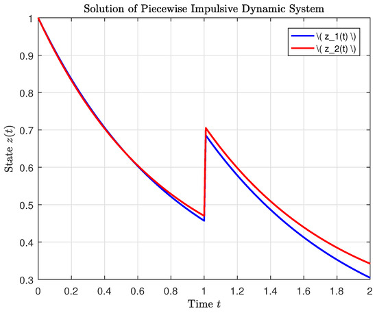
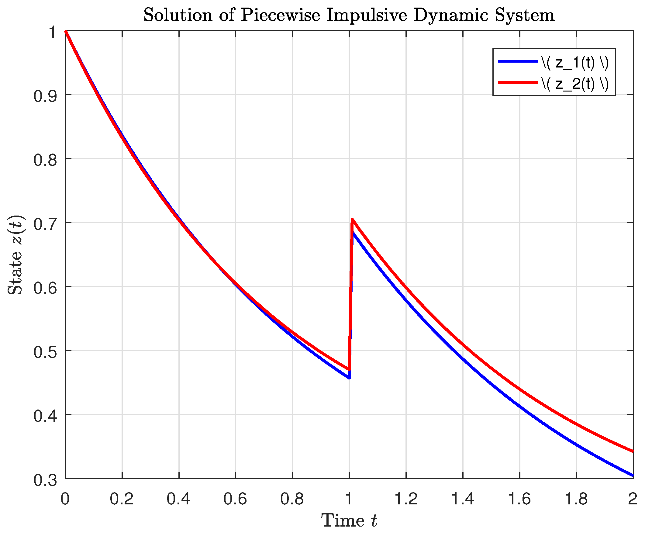
To illustrate the solution, we solve the system numerically using a simple Euler method for the time intervals $(0,1]$ and $(1,2]$.

1.

Initial Condition: $z(0)=\left[\begin{array}{c}1\\ 1\end{array}\right]$.

2.

Time Discretization: Use a step size $\Delta \mathfrak{t}=0.01$.

3.

Solution:

• For $\mathfrak{t}\in (0,1]$:

  $$z(\mathfrak{t}+\Delta t)=z(\mathfrak{t})+\Delta \mathfrak{t}\left(A_1(\mathfrak{t})z(\mathfrak{t})+F_1(\mathfrak{t},z(\mathfrak{t}))+\in {\mathfrak{t}}_0^{\mathfrak{t}}K(\mathfrak{t},\hslash )H_1(\hslash ,z(\hslash ))\Delta \hslash \right).$$
• At $t=1$, apply the impulsive effect:

  $$z(1^{+})=z(1^{-})+G_1(1,z(1^{-})).$$
• For $\mathfrak{t}\in (1,2]$:

  $$z(\mathfrak{t}+\Delta t)=z(\mathfrak{t})+\Delta t\left(A_2(\mathfrak{t})z(\mathfrak{t})+F_2(t,z(\mathfrak{t}))+{\int }_1^{\mathfrak{t}}K(t,\hslash )H_2(\hslash ,z(\hslash ))\Delta \hslash \right).$$

Figure 1 shows the numerical behaviour of the given system $z(\mathfrak{t})$.

Figure 1. $z\left(\mathfrak{t}\right)$.

6. Conclusions

In this paper, we study the existence of solutions for a class of nonlinear impulsive differential systems with integral boundary conditions on arbitrary time scales. We developed a generalized model with discrete and continuous behaviors based on the theory of time scales. The existence of unique and multiple solutions and stability of the system were proved using Banach and Schauder fixed point theorems. The controllability problem is reduced to a fixed point problem, and sharp conditions for control are derived. Simulations in different time domains confirmed the theoretical results.

The present research generalizes the known results and fills the gap in the existing literature by extending the controllability analysis to piecewise impulsive systems on time scales. The results of this work are of special interest in areas such as biology, engineering and economics, where impulsive effects and switching behavior are usual features of systems. This work provides a unified framework for controllability and stability, and practical tools for control design and management of complex dynamic systems. Extensions to infinite dimensional spaces could be considered in future work. Applications to emerging areas such as networked systems and artificial intelligence would further extend the impact of this work.

References

- Wonham, W. On pole assignment ble linear systems. IEEE Trans. Autom. Control 1967, 12, 660–665. [Google Scholar] [CrossRef] [Scilit]
- Helwa, M.-K.; Schoellig, A.P. On the construction of safe controllable regions for affine systems with applications to robotics. Automatica 2018, 98, 323–330. [Google Scholar] [CrossRef] [Scilit]
- Hussain, S.; Sarwar, M.; Shah, S.K.; Abodayeh, K.; De la Sen, M. Approximate controllability and existence results of the Sobolev-type fractional stochastic differential equations driven by a fractional Brownian motion. Fractal Fract. 2026, 10, 203. [Google Scholar] [CrossRef] [Scilit]
- Chaves-Silva, F.-W.; Zhang, X.; Zuazua, E. Controllability of evolution equations with memory. SIAM J. Control Optim. 2017, 55, 2437–2459. [Google Scholar] [CrossRef] [Scilit]
- Si, Y.; Wang, J.; Fečkan, M. Controllability of linear and nonlinear systems governed by Stieltjes differential equations. Appl. Math. Comput. 2020, 376, 125139. [Google Scholar] [CrossRef] [Scilit]
- Wang, J.; Luo, Z.; Fečkan, M. Relative controllability of semilinear delay differential systems with linear parts defined by permutable matrices. Eur. J. Control 2017, 38, 39–46. [Google Scholar] [CrossRef] [Scilit]
- Lu, X.; Li, H.; Wang, C.; Zhang, X. Stability analysis of positive switched impulsive systems with delay on time scales. Int. J. Robust Nonlinear Control 2020, 30, 6879–6890. [Google Scholar] [CrossRef] [Scilit]
- Hussain, S.; Sarwar, M.; Shah, S.K.; Abodayeh, K.; Ansari, K.J.; Promsakon, C.; Sitthiwirathham, T. A study on the controllability of Atangana–Baleanu–Caputo fractional neutral differential equations with delay. Chaos Solitons Fractals 2025, 201, 117365. [Google Scholar] [CrossRef] [Scilit]
- Bainov, D.; Simeonov, P.S. Impulsive Differential Equations: Periodic Solutions and Applications; CRC Press: Boca Raton, FL, USA, 1993; Volume 66. [Google Scholar]
- Yang, T.; Chua, L.O. Impulsive control and synchronization of nonlinear dynamical systems and application to secure communication. Int. J. Bifurc. Chaos Appl. Sci. Eng. 1997, 7, 645–664. [Google Scholar] [CrossRef] [Scilit]
- Lakshmikantham, V.; Simeonov, P.S. Theory of Impulsive Differential Equations; World Scientific: Singapore, 1989. [Google Scholar]
- Negi, S.S.; Abbas, S.; Malik, M.; Grace, S.R. New oscillation criteria for p-Laplacian dynamic equations on time scales. Rocky Mt. J. Math. 2020, 50, 659–670. [Google Scholar] [CrossRef] [Scilit]
- Wu, J.; Asamoah, B.; Kong, Z.; Ditterich, J. Exploring the suitability of piecewise-linear dynamical system models for cognitive neural dynamics. Front. Neurosci. 2025, 19, 1582080. [Google Scholar] [CrossRef] [Scilit]
- Kattan, D.A.; Hammad, H.A. Existence and stability results for piecewise Caputo–Fabrizio fractional differential equations with mixed delays. Fractal Fract. 2023, 7, 644. [Google Scholar] [CrossRef] [Scilit]
- Bianchini, G.; Paoletti, S. Linear fractional representations and L2-stability analysis of continuous piecewise affine systems. IEEE Control Syst. Lett. 2021, 5, 229–234. [Google Scholar] [CrossRef] [Scilit]
- Kumar, V.; Malik, M. Stability and controllability results of evolution system with impulsive condition on time scales. Differ. Equ. Appl. 2019, 11, 543–561. [Google Scholar] [CrossRef] [Scilit]
- Kumar, V.; Djemai, M.; Defoort, M.; Malik, M. Total controllability results for a class of time-varying switched dynamical systems with impulses on time scales. Asian J. Control 2022, 24, 474–482. [Google Scholar] [CrossRef] [Scilit]
- Nasser, B.B.; Djemai, M.; Defoort, M.; Laleg-Kirati, T.M. Time scale observability and constructibility of linear dynamic equations. Int. J. Control 2022, 95, 1994–2004. [Google Scholar] [CrossRef] [Scilit]
- Kumar, V.; Malik, M.; Djemai, M. Results on abstract integro hybrid evolution system with impulses on time scales. Nonlinear Anal. Hybrid Syst. 2021, 39, 100986. [Google Scholar] [CrossRef] [Scilit]
- Algolam, M.S.; Hussain, S.; Younis, B.A.; Osman, O.; Muflh, B.; Aldwoah, K.; Eljaneid, N. Stability and controllability analysis of stochastic fractional differential equations under integral boundary conditions driven by Rosenblatt process with impulses. Fractal Fract. 2025, 9, 146. [Google Scholar] [CrossRef] [Scilit]
- Kumar, V.; Djemai, M. Existence, stability and controllability of piecewise impulsive dynamic systems on arbitrary time domain. Appl. Math. Model. 2023, 117, 529–548. [Google Scholar] [CrossRef] [Scilit]
- Bohner, M.; Peterson, A. Dynamic Equations on Time Scales: An Introduction with Applications; Birkh”auser: Boston, MA, USA, 2001. [Google Scholar]
- Bohner, M.; Peterson, A. Advances in Dynamic Equations on Time Scales; Birkh”auser: Boston, MA, USA, 2003. [Google Scholar]
- Lupulescu, V.; Younus, A. On controllability and observability for a class of linear impulsive dynamic systems on time scales. Math. Comput. Model. 2011, 54, 1300–1310. [Google Scholar] [CrossRef] [Scilit]
- Sarwar, M.; Rahmat, G.; Hussain, S.; Mufarrej, M.Y.B.; Abodayeh, K. Fixed point theorems for a subfamily of non-expansive evolution operators. Eur. J. Pure Appl. Math. 2025, 18, 6147. [Google Scholar] [CrossRef] [Scilit]
Disclaimer/Publisher’s Note: The statements, opinions and data contained in all publications are solely those of the individual author(s) and contributor(s) and not of MDPI and/or the editor(s). MDPI and/or the editor(s) disclaim responsibility for any injury to people or property resulting from any ideas, methods, instructions or products referred to in the content. |
© 2026 by the authors. Licensee MDPI, Basel, Switzerland. This article is an open access article distributed under the terms and conditions of the Creative Commons Attribution (CC BY) license.