Article

Bifurcation, Phase Portrait and Traveling Wave Solution of Aizhan–Gudekli–Nurshuak–Zhanbota Equation


College of Computer Science, Chengdu University, Chengdu 610106, China
*
Author to whom correspondence should be addressed.
Axioms 2026, 15(6), 434; https://doi.org/10.3390/axioms15060434
Submission received: 10 May 2026 / Revised: 9 June 2026 / Accepted: 10 June 2026 / Published: 11 June 2026

Abstract

This paper investigates the bifurcation, phase portrait, and traveling wave solutions of the Aizhan–Gudekli–Nurshuak–Zhanbota equation. By performing a simple linear transformation on the solution of the equation and applying the traveling wave transformation, the original equations are reduced to a system of ordinary differential equations. Through a qualitative analysis of the resulting two-dimensional dynamical system, the types and stability of equilibrium points are classified under various parameter conditions. Using both the dynamical system method and the complete discriminant system, multiple families of exact traveling wave solutions including solitary, kink, and periodic wave solutions are derived for different parameter ranges. Numerical simulations using Maple software are performed to visualize selected solutions. The obtained solutions are novel and provide a theoretical foundation for understanding the physical applications of the equation.

1. Introduction

Research on complex-valued nonlinear partial differential equations [1,2,3,4,5] has become a prominent frontier in mathematical physics and applied mathematics. These equations, characterized by complex field variables, naturally arise in fields, where they describe the evolution of wave envelopes and coherent structures [6]. Key models in this domain include the foundational nonlinear Schrödinger equation [7], along with significant generalizations like the high-dispersion Lakshmanan–Porsezian–Daniel equation [8], the Fokas–Lenells equation [9], and the coupled Twin-Core system [10]. Current research focuses on uncovering novel soliton dynamics [11], rogue waves [12,13], and modulation instability [14] while extending the analysis to non-autonomous, stochastic, and higher-dimensional settings [15]. Advances in the inverse scattering technique [16], dynamical system method [17,18,19], Riemann–Hilbert method [20], and neural network method [21,22] are driving the field forward, deepening our understanding of nonlinear wave phenomena and enabling new applications in photonics and beyond [23,24,25].
In this paper, we will consider the following Aizhan–Gudekli–Nurshuak–Zhanbota (AGNZ) equation [26,27]
i Q t + Q x t + i V Q x i 2 Q 2 R t + ( 1 1 2 R Q ) V Q = 0 , i R t R x t + i V R x i 2 R 2 Q t ( 1 1 2 R Q ) V R = 0 , V x + 1 2 ( R Q ) t = 0 ,
where Q = Q ( x , t ) and R = R ( x , t ) are unknown complex functions, and V = V ( x , t ) represents a real function. AGNZ equations are a class of nonlinear evolution equations with coupled complex-valued fields and real-valued potential fields, which have potential applications in wave phenomena and nonlinear physics.
To simplify Equation (1), we make the following assumptions
R = ε Q ¯ ,
where Q ¯ stands for the complex conjugate of Q, and ε = ± 1 .
Next, substituting Equation (2) into Equation (1), Equation (1) can be rewritten as
i Q t + Q x t + i ( V Q ) x + i ε 2 | Q 2 | Q t + ( 1 ε 2 | Q 2 | ) V Q = 0 , V x = ε 2 ( | Q | 2 ) t .
In reference [26], Ibrahim and his collaborators obtained the traveling wave solutions of Equation (1) by using the modified exp- [ ξ ] -expansion method and the modified simple equation method. In reference [27], Afridi used the N-fold Darboux transformation to study the soliton and rogue wave solutions of Equation (1). Compared with the existing literature (see Refs. [26,27]), this paper not only considers the traveling wave solution of Equation (1) but also obtains the Jacobian function solution. Moreover, this article also discusses the dynamic behavior of Equation (1) and its perturbation system, which have not been reported in the existing literature.
The rest of this article is organized as follows: In Section 2, we use a traveling wave transformation to simplify Equation (3) into ordinary differential equations. In Section 3, the qualitative behavior of Equation (8) and its perturbed system is analyzed. In Section 4, we derive the wave-making solution of Equation (3) based on the method of dynamic system analysis. In Section 5, we use the method of the complete discriminant system to derive the traveling wave solution to Equation (3). In Section 6, we use Maple mathematical software to draw graphs of some solutions. In Section 7, we present the results and discussion. In Section 8, a brief summary is presented.

2. Mathematical Derivation

Firstly, we present a complex-valued traveling wave transformation
Q ( x , t ) = q ( ξ ) e i ϑ , V ( x , t ) = v ( ξ ) , ξ = x + c t , ϑ = x + σ t + ϑ 0 ,
where q and v stand for the wave amplitude, c denotes the soliton speed, ϑ represents the phase portion, σ stands for the wave number, and ϑ 0 represents the phase constant.
Inserting Equation (4) into Equation (3) and splitting the real and imaginary parts respectively, we can obtain the following equations
c q 2 σ q ε 2 ( σ + v ) q 3 = 0 , ( 2 c + σ + v ) q c ε 2 q 2 q = 0 .
Integrating the second equation of Equation (5) yields
v = c ε 2 q 2 2 c σ .
Inserting Equation (6) into the first equation of Equation (5), we obtain
q 1 4 q 5 + ε q 3 2 σ c q = 0 .

3. Qualitative Analysis of Equation (7)

Let d q d ξ = z . Thus, we can obtain a two-dimensional dynamical system of Equation (7) as follows
d q d ξ = z , d z d ξ = 1 4 q ( q 4 + 4 ε q 2 8 σ c ) ,
with Hamiltonian system
H ( q , z ) = 1 2 z 2 1 24 q 6 ( ξ ) ε 4 q 4 ( ξ ) + σ c q 2 ( ξ ) = h ,
where h is an integral constant.
According to the theory of planar dynamical systems, consider the function
F ( q ) = 1 4 q ( q 4 + 4 ε q 2 8 σ c ) ,
Δ = 16 ( 1 + 2 σ c ) , and denote by q j ( j = 0 , 1 , 2 ) the real root of F ( q j ) = 0 .
Let E j ( q j , 0 ) be the equilibrium point of system (8). The coefficient matrix at this equilibrium is
M ( q j , 0 ) = 0 1 F ( q j ) 0 .
Furthermore, define
J ( q j , y ) = det M ( q j , 0 ) = F ( q j ) .
Based on the linearization theory of the power system, relevant conclusions such as the type of equilibrium point can be obtained.
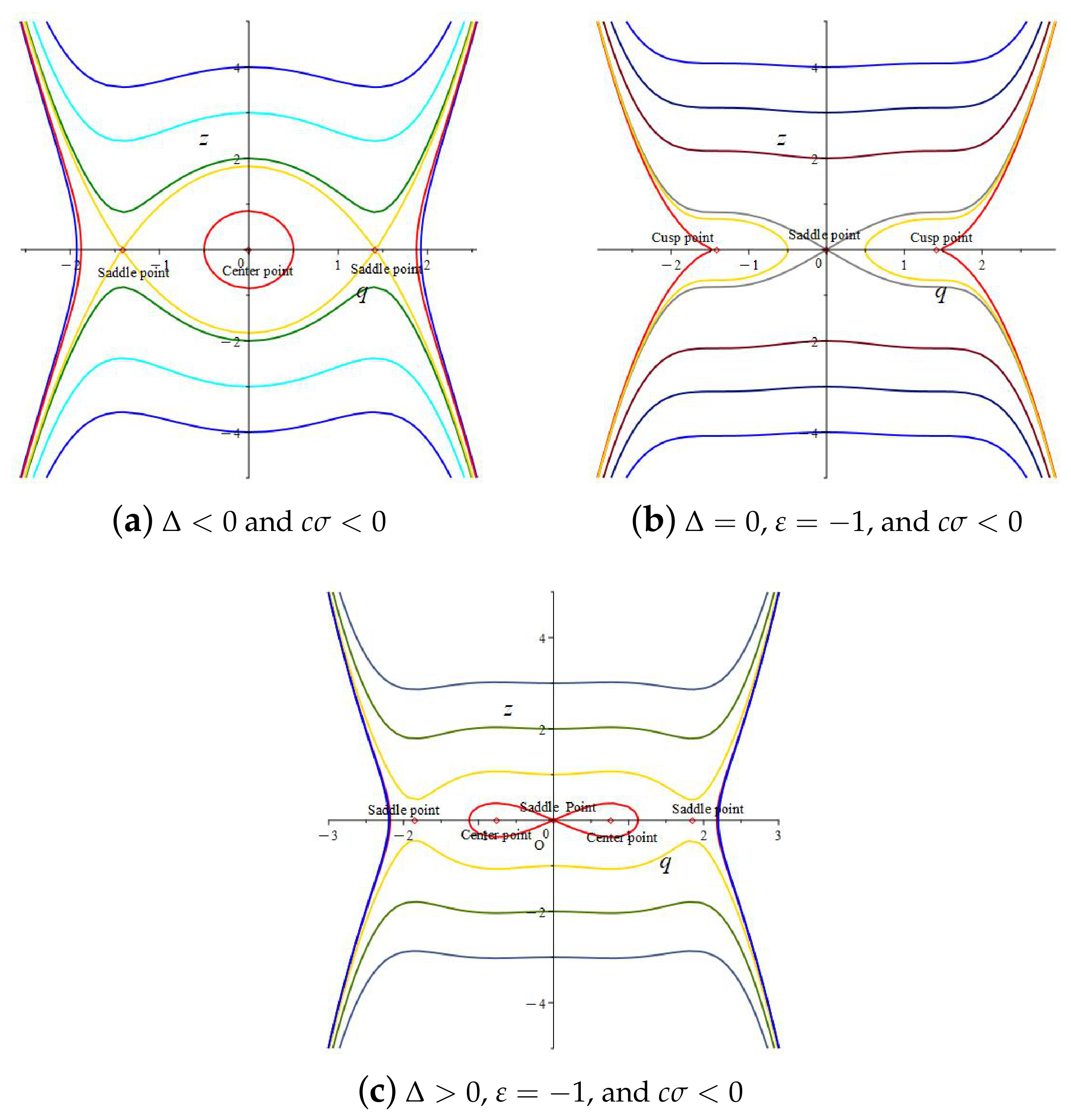
(I) Δ < 0 or Δ > 0 , ε > 0 , and σ c < 0 :
If J ( 0 , 0 ) < 0 , E 0 ( 0 , 0 ) , the unique equilibrium of Equation (8), acts as a saddle point, as shown in Figure 1a.
(II) Δ = 0 , ε = 1 , and σ c < 0 :
If J ( 0 , 0 ) < 0 , the equilibrium point E 0 ( 0 , 0 ) is a saddle point, as shown in Figure 1b.
If E 1 ± ( ± 2 , 0 ) , the points E 1 ± ( ± 2 , 0 ) become cusp points. Additionally, the Poincaré index of these equilibria equals zero.
Here, E 0 ( 0 , 0 ) and E 1 ± ( ± 2 , 0 ) are three equilibrium points of Equation (8).
(III) Δ > 0 , ε = 1 , and σ c < 0 :
If J ( 0 , 0 ) > 0 , the equilibrium point E 0 ( 0 , 0 ) is a saddle point (as illustrated in Figure 1c).
If J ± 2 ε + 2 1 + 2 σ c , 0 < 0 , the points E 2 ± ± 2 ε + 2 1 + 2 σ c , 0 act as center points, as shown in Figure 1c.
Notably, E 0 ( 0 , 0 ) and E 2 ± ± 2 ε + 2 1 + 2 σ c , 0 constitute the three equilibrium points of Equation (8).
Remark 1. 
In (I) (single saddle point), there are homoclinic orbits connecting saddle points in phase space, corresponding to bright soliton solutions (such as Q 1 ( x , t ) in Section 4). In (III) (where the center point is surrounded by two saddle points), the closed orbit around the center point corresponds to the periodic wave solution (such as Q 3 ( t , x ) in Section 4). The heteroclinic orbit connecting the two saddle points corresponds to a twisted/anti-twisted wave solution Q 2 ( t , x ) , Q 6 ( t , x ) in Section 4.
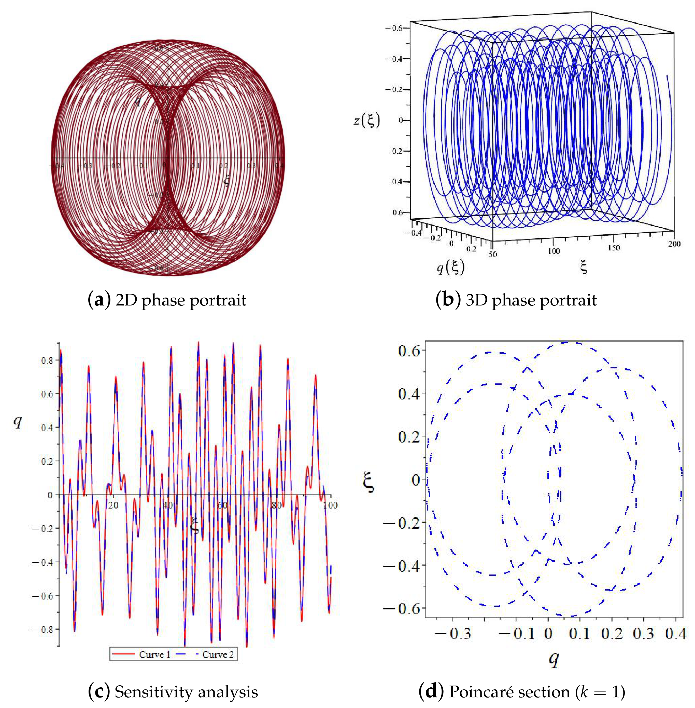
In this section, we will investigate the two-dimensional planar dynamical system (8) that includes a perturbation term.
d q d ξ = z , d z d ξ = 1 4 q ( q 4 + 4 ε q 2 8 σ c ) + A cos ( k ξ ) .
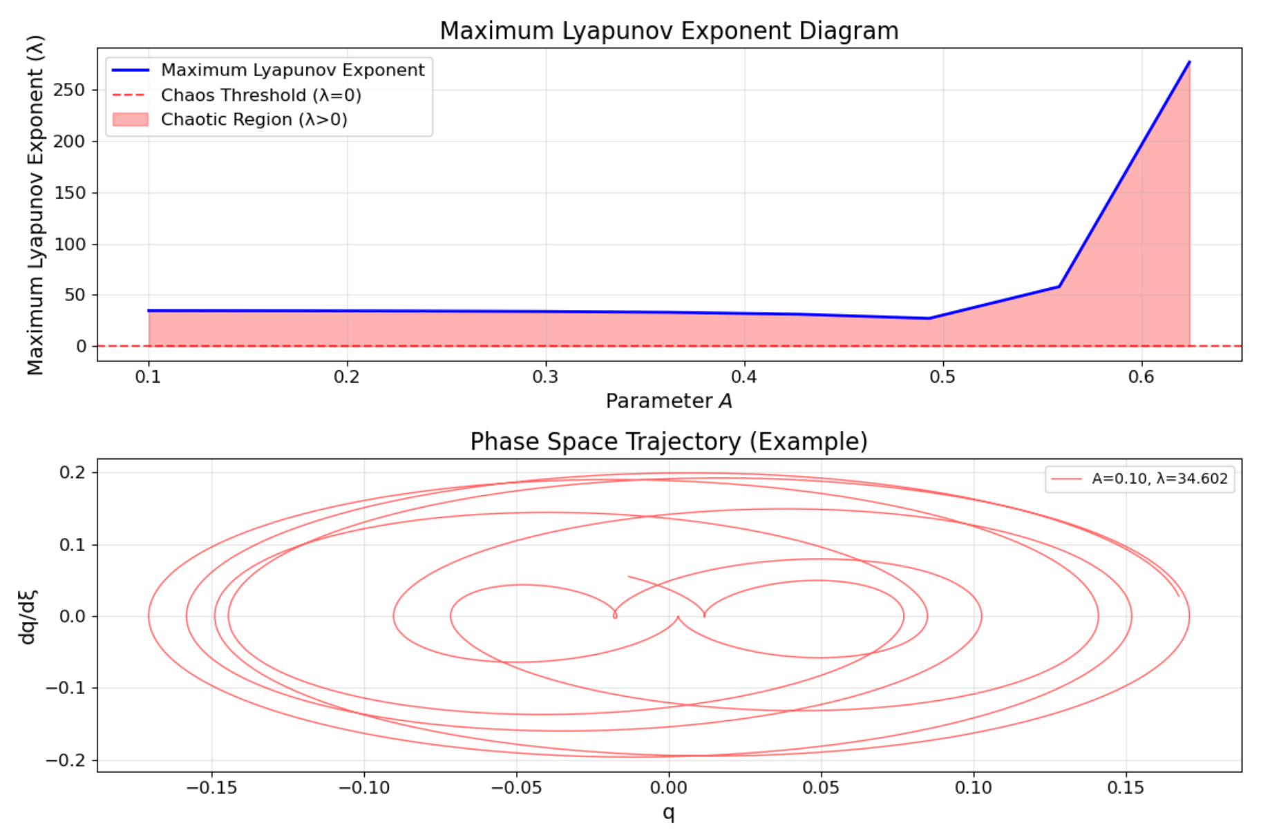
As shown in Figure 2 and Figure 3, we plotted the two-dimensional phase diagram, three-dimensional phase diagram, sensitivity map, Poincaré section and maximum Lyapunov exponent of system (13). In Figure 3, when the curve is above the horizontal zero line, there is only a very small difference in the initial conditions of the system (13), and the long-term motion of the system will quickly diverge towards completely different states. When the curve is below the zero line, the system (13) eventually converges to a stable periodic motion or stationary state, and its behavior is predictable.

4. Traveling Wave Solutions of Equation (1) Under Method of Dynamical System

Set F h ( q ) = 1 24 q 6 ( ξ ) + ε 4 q 4 ( ξ ) 2 σ c q 2 ( ξ ) + h , and h 1 = F 0 ( q 1 ± ) , where q 1 ± = ± 2 ε + 2 1 + 2 σ c .

4.1. ε < 0 and 3 8 < σ c < 0

(i) If h = 0 , Equation (9) can be expressed in the equivalent form
y = ± 1 12 q 2 ( ρ 1 q 2 ) ( ρ 2 q 2 ) ,
where the roots ρ 1 , 2 are given by ρ 1 , 2 = 3 ε 9 + 24 σ c .
Substituting Equation (14) into the transformation d q d ξ = z and performing the integration yields two solitary wave solutions
Q 1 ( x , t ) = ± ρ 1 ρ 2 sech 2 ( ρ 1 ρ 2 12 ) 1 2 ( x + c t ) ρ 2 ρ 1 tanh 2 ( ρ 1 ρ 2 12 ) 1 2 ( x + c t ) e i ( x + σ t + ϑ 0 ) .
(ii) In the case where h = h 1 , Equation (9) can be recast as
y = ± 1 12 q 2 ( q 2 ρ 3 ) ( ρ 4 q 2 ) 2 ,
with the parameters defined as ρ 3 = 2 ε 4 1 + 2 σ c and ρ 4 = 2 ε + 4 1 + 2 σ c .
Integrating Equation (16) under the same substitution d q d ξ = z leads to two kink wave solutions
Q 2 ( x , t ) = ± ρ 3 ρ 4 tanh ( ρ 4 ( ρ 4 ρ 3 ) 12 ) 1 2 ( x + c t ) ρ 4 sech 2 ( ρ 4 ( ρ 4 ρ 3 ) 12 ) 1 2 ( x + c t ) ρ 3 e i ( x + σ t + ϑ 0 ) .
(iii) For h ( 0 , h 1 ) , Equation (26) can be rewritten as
y = ± 1 12 ( ρ 5 q 2 ) ( q 2 + ρ 6 ) ( ρ 7 q 2 ) ,
where ρ 6 = 2 ρ 5 + 12 ε + ( 2 ρ 5 + 12 ε ) 2 8 ( 2 ρ 5 2 + 12 ε ρ 5 48 σ c ) 4 , ρ 7 = 2 ρ 5 12 ε + ( 2 ρ 5 + 12 ε ) 2 8 ( 2 ρ 5 2 + 12 ε ρ 5 48 σ c ) 4 , and ρ 5 ( ρ 3 , ρ 2 ) .
Substituting Equation (18) into d q d ξ = z and performing the integration, we derive two periodic wave solutions
Q 3 ( x , t ) = [ ρ 5 ρ 6 sn 2 ( ρ 7 ( ρ 5 + ρ 6 ) 12 ( x + c t ) , ρ 5 ( ρ 6 + ρ 7 ) ρ 7 ( ρ 5 ρ 6 ) · ρ 6 + ρ 5 cn 2 ( ρ 7 ( ρ 5 + ρ 6 ) 12 ( x + c t ) , ρ 5 ( ρ 6 + ρ 7 ) ρ 7 ( ρ 5 ρ 6 ) ) ) 1 ] 1 2 e i ( x + σ t + ϑ 0 ) .

4.2. ε < 0 and σ c = 9 8

If h = h 1 , Equation (9) can be rewritten as
y = ± 1 12 q q 2 + 3 ε .
Substituting Equation (20) into d q d ξ = z and integrating, we obtain
Q 4 ± ( x , t ) = ± 3 3 2 ( 1 + tanh 3 3 ( x + c t ) + ln 3 3 ) ) e i ( x + σ t + ϑ 0 ) .
Q 5 ± ( x , t ) = ± 3 3 2 ( 1 tanh 3 3 ( x + c t ) ln 3 3 ) ) e i ( x + σ t + ϑ 0 ) .

4.3. ε < 0 and 1 2 < σ c < 3 8

If h = h 1 , Equation (9) can be rewritten as
y = ± 1 12 q 2 ρ 3 ρ 4 q 2 2 .
Substituting Equation (23) into d q d ξ = z and integrating, we derive two solitary wave solutions
Q 6 ± ( x , t ) = ± ρ 3 ρ 4 ρ 4 + ( ρ 3 ρ 4 ) tanh 2 ρ 4 ( ρ 4 ρ 3 ) 12 ( x + c t ) e i ( x + σ t + ϑ 0 ) .

5. Traveling Wave Solutions of Equation (1) Under Method of Complete Discriminant System

We multiply both sides of Equation (7) by d u d ξ and then integrate it once to obtain
d q d ξ 2 = 1 12 q 6 ε 2 q 4 + 2 σ c q 2 + d ,
where d is the integral constant.
Next, we can proceed with the transformation f ( ξ ) = q 2 ( ξ ) . Then, Equation (25) becomes
± 1 3 ( ξ ξ 0 ) = d f f ( f 3 + c 2 f 2 + c 1 f + c 0 ) ,
where c 2 = 6 ε , c 1 = 24 σ c , and c 0 = 12 d .
To simplify the calculation, we can denote the third-order polynomial as
G ( f ) = f 3 + c 2 f 2 + c 1 f + c 0 .
Then, its complete discrimination system is
Δ = 27 2 c 2 3 27 + c 0 c 2 c 1 3 2 4 c 1 c 2 2 3 3 , D 1 = c 1 c 2 2 3 .
Based on Liu’s method [28], we can obtain the traveling wave solution of Equation (3).
Case I. If Δ = 0 , D 1 < 0 , then Equation (27) can be written as G ( f ) = ( f a ) 2 ( f b ) , where both a and b are real numbers, a b , and b > 0 .
When a > b and f > b , or when a < 0 and f < 0 , it can be obtained from Equation (26) that
± 1 3 ξ ξ 0 = 1 a ( a b ) ln a ( f b ) f ( a b ) 2 | f a | .
When a > b and f < 0 , or when a < f < b , it can be obtained from Equation (26) that
± 1 3 ξ ξ 0 = 1 a ( a b ) ln a ( f b ) + f ( b a ) 2 | f a | .
When b > a > 0 , it can be obtained from Equation (26) that
± 1 3 ξ ξ 0 = 1 a ( b a ) arcsin a ( f b ) + f ( a b ) b | f a | .
Case II. If Δ = 0 , D 1 = 0 , then Equation (27) can be written as G ( f ) = ( f α ) 3 , where α is a real number.
When f > α and f > 0 , or when f < α and f < 0 , it can be obtained from Equation (1)
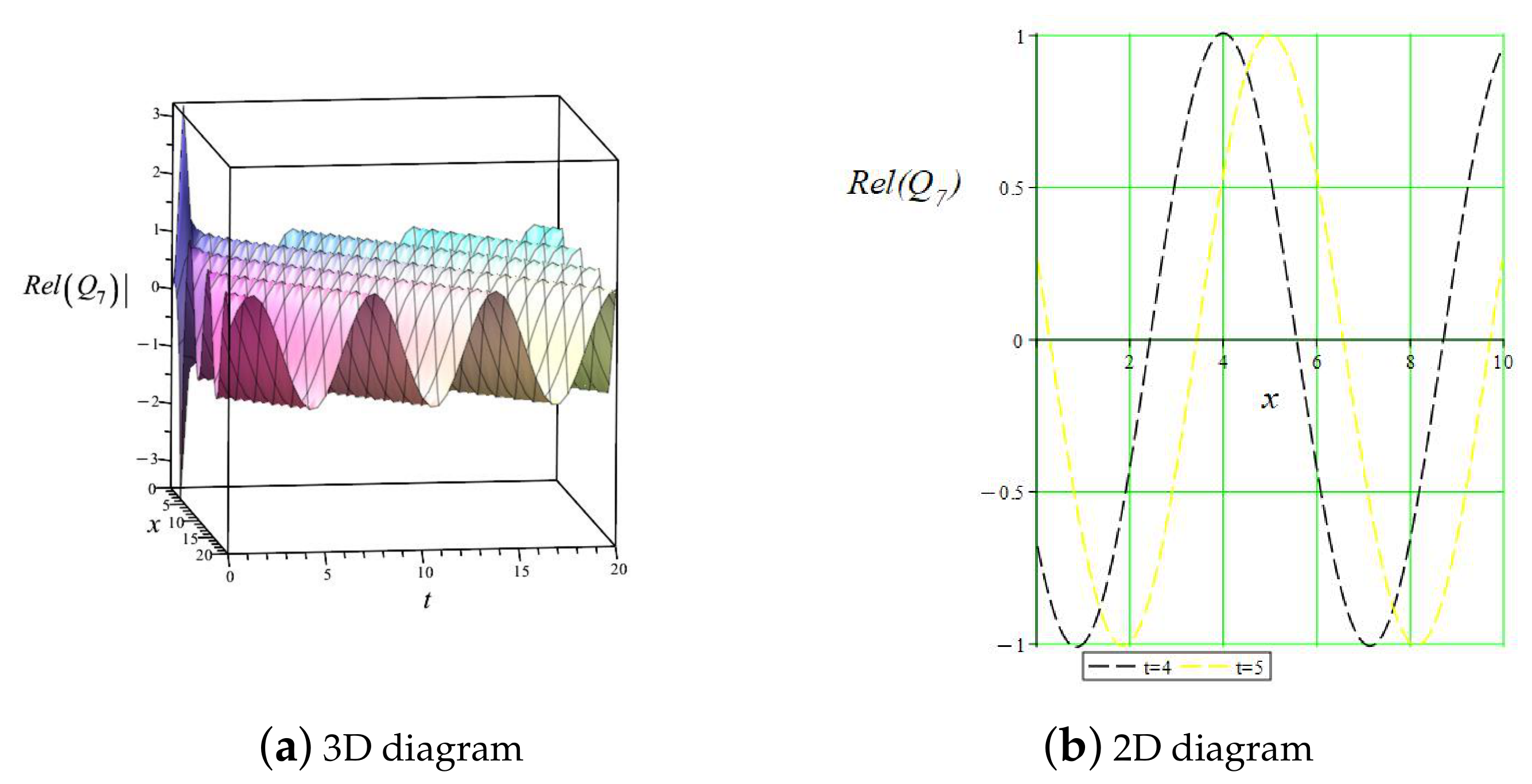
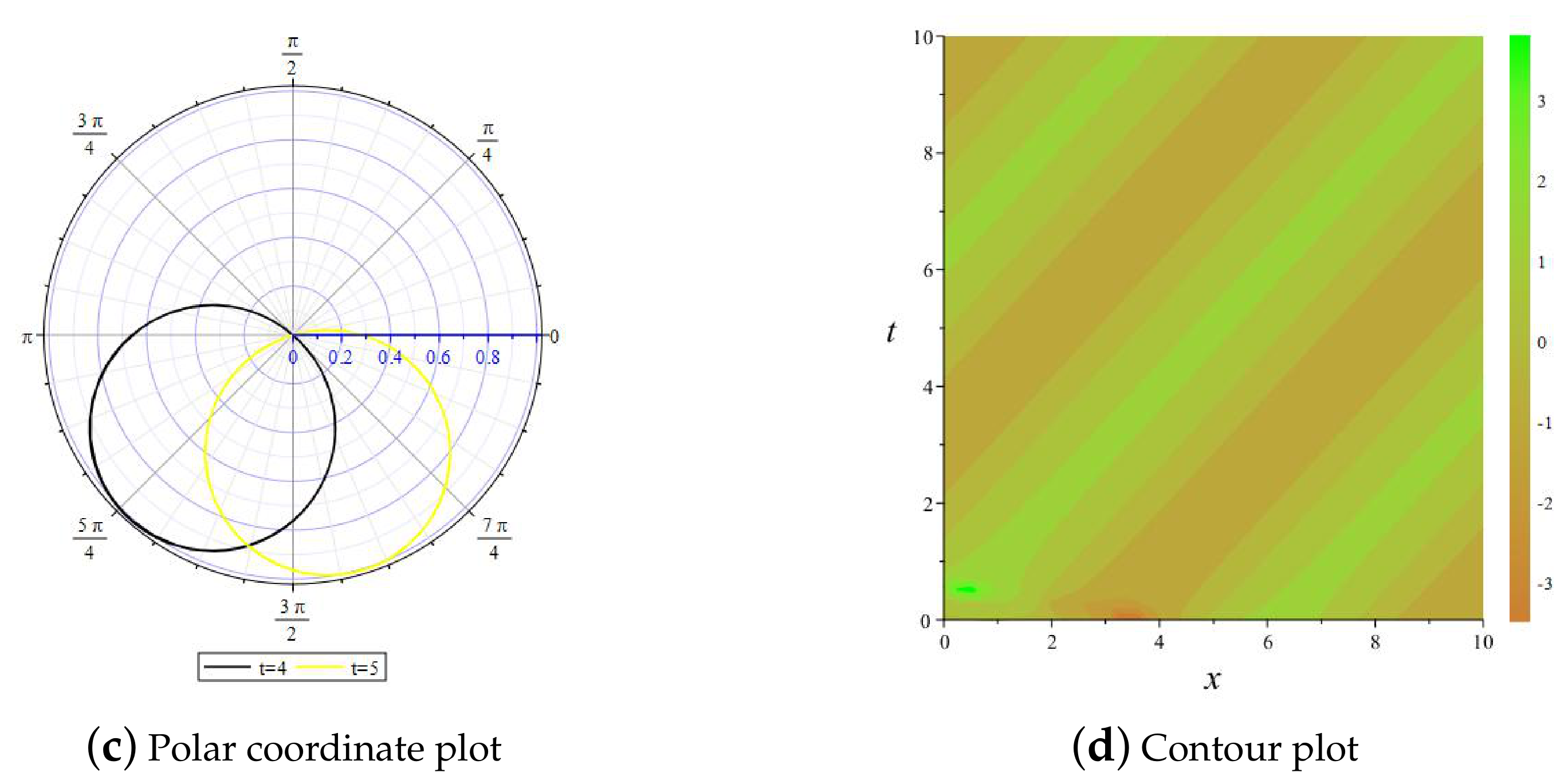
Q 7 ( x , t ) = ± 12 α α 2 ( x + c t ξ 0 ) 2 12 + α · e i ( x + σ t + ϑ 0 ) .
Case III. If Δ > 0 , D 1 < 0 , then Equation (27) can be written as G ( f ) = ( f m ) ( f n ) ( f l ) , where m, n and l are real numbers, and 0 < m < n < l .
When 0 < f < l , it can be obtained from Equation (1) that
Q 8 ( x , t ) = ± l m sn 2 n ( m l ) 1 12 ( x + c t ξ 0 ) , β l sn 2 n ( m l ) 1 12 ( x + c t ξ 0 ) , β ( m l ) e i ( x + σ t + ϑ 0 ) ,
Q 9 ( x , t ) = ± l ( m n ) sn 2 n ( m l ) 1 12 ( x + c t ξ 0 ) , β n ( m l ) ( m n ) sn 2 n ( m l ) 1 12 ( x + c t ξ 0 ) , β ( m l ) e i ( x + σ t + ϑ 0 ) ,
where β 2 = l ( m n ) n ( m l ) .
Case IV. If Δ < 0 , then Equation (27) can be written as G ( f ) = ( f γ 1 ) [ ( f γ 2 ) 2 + γ 3 2 ] , where γ 1 , γ 2 and γ 3 are real numbers, and γ 1 > 0 , γ 2 , γ 3 > 0 . So, it can be obtained from Equation (1) that
Q 10 ( x , t ) = ± a 1 cn 2 γ 3 m 1 γ 1 6 m m 1 ( x + c t ξ 0 ) , m + a 2 a 3 cn 2 γ 3 m 1 γ 1 6 m m 1 ( x + c t ξ 0 ) , m + a 4 e i ( x + σ t + ϑ 0 ) ,
where a 1 = 1 2 γ 1 ( a 3 a 4 ) , a 2 = 1 2 γ 1 ( a 4 a 3 ) , a 3 = γ 1 γ 2 γ 3 m 1 , a 4 = γ 1 γ 2 γ 3 m 1 , a 5 = γ 3 2 γ 2 ( γ 1 γ 2 ) γ 1 γ 3 , m 1 = a 5 ± a 5 2 + 1 and m 2 = 1 1 + m 1 2 .

6. Numerical Simulation

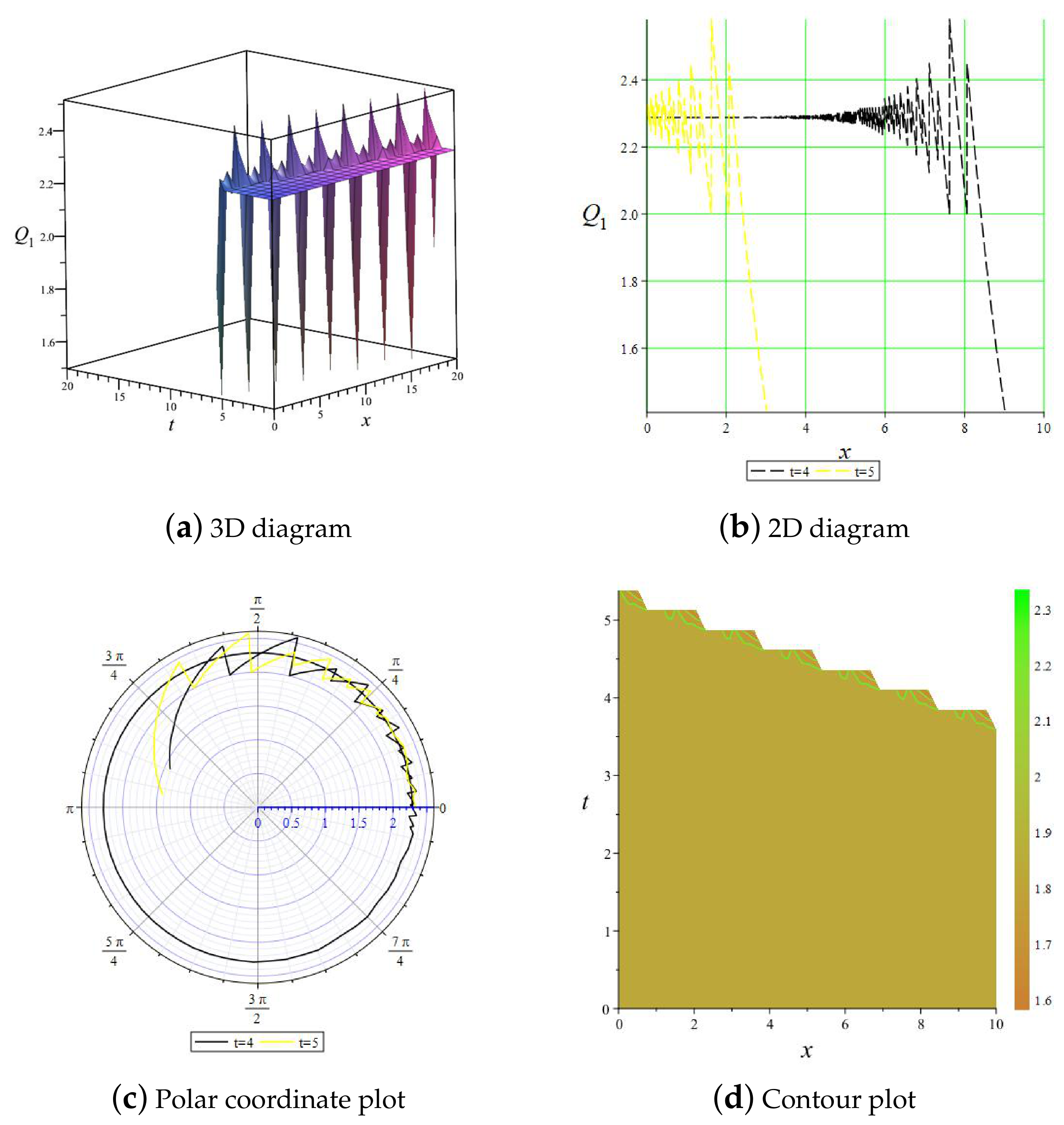
When ε = 1 , c = 6 , σ = 1 , ϑ 0 = 0 , we plot a 3D graphic, 2D graphic, polar plot and contour plot of the solution Q 1 ( t , x ) , as shown in Figure 4. Figure 4 shows the evolution of the solitary wave solution Q 1 ( t , x ) , and its three-dimensional and two-dimensional profiles and contour map jointly confirm that the solution has a localized and stable bell-shaped waveform, which corresponds to the physical form of the homoclinic orbit in Figure 1, namely a standard bright soliton. When c 0 = 1 , c 1 = 3 , c 2 = 3 , α = 1 , c = 1 , ϑ 0 = 0 , we plot a 3D graphic, 2D graphic, polar plot and contour plot of the solution Q 7 ( t , x ) , as shown in Figure 5. Figure 5 shows a graph of the rational functional solution Q 7 ( t , x ) , whose waveform characteristics are significantly different from Q 7 ( t , x ) , exhibiting smoother peaks and algebraic decay characteristics. Figure 4a and Figure 5b show the three-dimensional evolution of solution Q 1 and Q 7 over time t and space x. Figure 4b and Figure 5b represent the distribution of Q 1 and Q 7 with x at different times t. Figure 4c and Figure 5c show the distribution of polar coordinates of the solution at t = 4 and t = 5 . Figure 4d and Figure 5d show the distribution of solution Q 1 and Q 7 displayed by the gambler in the time and space planes with different colors.

7. Results and Discussion

This paper investigated the traveling wave solutions and dynamic behavior of the AGNZ equation using both the complete discriminant system method and the planar dynamical system analysis method. The traveling wave solutions of the AGNZ equation were obtained through the complete discriminant system method, including Jacobian function solutions, hyperbolic function solutions, trigonometric function solutions, rational function solutions, etc. The dynamic behavior of a two-dimensional planar dynamical system was obtained using the dynamical system method while also considering the dynamic behavior of its perturbed system. Compared with the existing literature (see [26,27]), this study provided a more general Jacobian function solution and also obtained the dynamic behavior of two-dimensional dynamical systems, which have not been reported in the previous literature. The biggest innovation of this article is to reduce the original equations by introducing a simplified relationship R = ε Q ¯ and then use a complex-valued traveling wave transformation to transform partial differential equations into ordinary differential equations. By linearizing and analyzing the Jacobian matrix of the obtained planar dynamical system, the system characterizes the types of equilibrium points, phase diagram topology, and bifurcation behavior in different parameter regions. Specifically, under the influence of disturbance terms, the system exhibits more diverse dynamic patterns. Multiple types of analytical traveling wave solutions are successfully derived, and their explicit expressions are given. With the help of Maple mathematical software, three-dimensional graphics, two-dimensional profiles, polar coordinates, and contour lines are visualized for solutions under typical parameters, intuitively demonstrating the morphology and propagation characteristics of our understanding.

8. Conclusions

In this paper, we studied the bifurcation, phase portrait, and traveling wave solutions of AGNZ equations. By employing methods from planar dynamical system theory and the complete discriminant system, we conducted a qualitative analysis of the corresponding traveling wave system, classified its equilibrium points, and obtained a series of exact traveling wave solutions including solitary, kink, and periodic wave solutions under different parameter conditions. We also used Maple software (https://www.maplesoft.com/) to perform numerical simulations and visualize some of the obtained solutions. Additionally, we point out that these solutions are novel and can provide a theoretical basis for understanding the physical applications of the equation. Finally, we indicate that the two-dimensional dynamical system considered in this study features a fifth-order polynomial and suggest that future research could involve more complex and higher-order dynamical systems.

Author Contributions

Software, J.W.; writing—original draft preparation, Z.L.; writing—review and editing, Z.L. All authors have read and agreed to the published version of the manuscript.

Funding

This research received no external funding.

Data Availability Statement

Data are contained within the article.

Conflicts of Interest

The authors declare no conflicts of interest.

References

  1. Yokuş, A.; Durur, H.; Ekici, M.H. Effect of diffusion parameters on traveling wave solutions of singular perturbed Boussinesq equation. An. Int. J. Optim. Control Theor. Appl. 2025, 15, 343–353. [Google Scholar] [CrossRef]
  2. Babaogulu, M.; Dipesh; Kumar, P. Investigation of stability and oscillatory behavior of alle-lochemical influence on plants in time delay differential equation model. Trans. Comput. Model. Intell. Syst. 2025, 1, 10013. [Google Scholar] [CrossRef]
  3. Hussain, A.; Chaudhary, U.A.; Junaid-U-Rehman, M.; Jhangeer, A. Stability, sensitivity, chaotic be-havior, and soliton solution of the perturbed Kaup-Newell equation. Ain Shams Eng. J. 2026, 17, 104097. [Google Scholar] [CrossRef]
  4. Tang, L. Bifurcation analysis, chaotic behavior, cubic-quartic optical solitons and phase portraits for the nonlinear coupled Kaup-Newell equation in birefringent fibers. Math. Methods Appl. Sci. 2026, 49, 239–253. [Google Scholar] [CrossRef]
  5. Xu, Z.; Hong, Q.; Wang, Y.; Gong, Y. Highly efficient semi-implicit structure-preserving algorithms for preserving the symmetry and quadratic invariants of complex-valued nonlinear partial differential equations. J. Comput. Phys. 2026, 558, 114868. [Google Scholar] [CrossRef]
  6. Mahmood, S.S.; Murad, M.A.S. Optical solutions of weakly nonlocal media for nonlinear conformable Schrödinger equation by extended simplest equation method. Phys. Lett. A 2025, 560, 130936. [Google Scholar] [CrossRef]
  7. Tang, L. Qualitative analysis, traveling wave solutions and chaotic behavior for the perturbed Schrödinger-Hirota equation with cubic-quintic-septic law of self-phase modulation. Mod. Phys. Lett. B 2025, 40, 2550170. [Google Scholar] [CrossRef]
  8. Lin, B.; Zhang, Y. Riemann–Hilbert problem with arbitrary order poles for the vector Laksh-manan–Porsezian–Daniel equation. Phys. A Stat. Mech. Its Appl. 2026, 690, 131459. [Google Scholar] [CrossRef]
  9. Wang, L.; Tian, S. A novel Transformer-Enhanced PINN approach to the Fokas–Lenells equa-tion: Forward and inverse problems. Chaos Solitons Fractals 2026, 204, 117787. [Google Scholar] [CrossRef]
  10. Rabie, W.B.; Ahmed, H.M. Construction cubic-quartic solitons in optical metamaterials for the perturbed twin-core couplers with Kudryashov’s sextic power law using extended F-expansion method. Chaos Solitons Fractals 2022, 160, 112289. [Google Scholar] [CrossRef]
  11. El-Nabulsi, R.A.; Anukool, W. Soliton dynamics under fractional action-induced non-Markovian dissipation and memory effects. Phys. A Stat. Mech. Its Appl. 2026, 693, 131562. [Google Scholar] [CrossRef]
  12. Fan, F.; Yu, G. Breathers and rogue waves on the background of periodic traveling waves in the Hirota equation. Phys. D Nonlinear Phenom. 2026, 492, 135229. [Google Scholar] [CrossRef]
  13. Qiu, T.; Wang, M.; Wang, Z.; Liu, X.-K.; Sun, J. Modulational instability, rogue waves and multi-pole solitons for the fifth-order reverse space-time nonlinear Schrödinger equation. Phys. D Nonlinear Phenom. 2026, 488, 135101. [Google Scholar] [CrossRef]
  14. Arnous, A.H.; Hosseini, K.; Murad, M.A.S.; Kumar, S. Soliton structures, modulational instability, and chaotic dynamics of the coupled Schrödinger—Boussinesq equation. Chaos Solitons Fractals 2026, 206, 117969. [Google Scholar] [CrossRef]
  15. Wang, Z.; Zhang, L. Finite fractal dimension of random attractor for stochastic non-autonomous strongly damped wave equation. Comput. Math. Appl. 2018, 75, 3343–3357. [Google Scholar] [CrossRef]
  16. Zhang, F.; Han, P.; Zhang, Y. Inverse scattering transform for the focusing two-component Hirota equation with nonzero boundary conditions. J. Math. Anal. Appl. 2026, 554, 129941. [Google Scholar] [CrossRef]
  17. Wang, J.; Li, Z. The impact of standard Wiener process on the qualitative analysis and traveling wave solutions of stochastic nonlinear Kodama equation in the Stratonovich sense. AIMS Math. 2025, 10, 24997–25010. [Google Scholar] [CrossRef]
  18. Farooq, F.B.; Raza, N.; Shahbaz, M.; Ali, S.; Bayram, M. A comprehensive study of qualitative analysis and soliton dynamics related to kairat-II-X-type equation. Ain Shams Eng. J. 2026, 17, 104172. [Google Scholar] [CrossRef]
  19. Li, Z.; Hussain, E. Bifurcation analysis and chaotic behaviors of and a traveling-wave solution to the Zhiber–Shabat Equation with a truncated M-Fractional derivative. Fractal Fract. 2026, 10, 335. [Google Scholar] [CrossRef]
  20. Hu, B.; Shen, Z.; Zhang, L. The nonlocal generalized nonlinear Schrödinger equation with step-like initial data via the Riemann–Hilbert method. Appl. Math. Lett. 2026, 179, 109943. [Google Scholar] [CrossRef]
  21. Li, Z. Solving the exactly explicit solutions of the conformable space-time fractional Phi-4 equation via neural networks method. Phys. Lett. A 2026, 581, 131535. [Google Scholar] [CrossRef]
  22. Li, Z.; Wu, M.; Hussain, E.; Yildirim, Y. Exactly explicit solutions of (2+1)-dimensional conformable fractional diffusive Predator–Prey model via neural networks method. Front. Phys. 2026, 14, 1824530. [Google Scholar] [CrossRef]
  23. Evirgen, F.; Özdemir, N. Multistage adomian decomposition method for solving NLP problems over a nonlinear fractional dynamical system. J. Comput. Nonlinear Dyn. 2011, 6, 021003. [Google Scholar] [CrossRef]
  24. Shams, M. Theoretical advances in two-step iterative schemes fornonlinear problems. Trans. Comput. Model. Intell. Syst. 2025, 1, 10011. [Google Scholar] [CrossRef]
  25. Tang, C.; Li, X.; Wang, Q. Solvability of indefinite stochastic LQ optimal control problems for jump diffusion models. J. Dynamcial Control Syst. 2026, 32, 9. [Google Scholar] [CrossRef]
  26. Ibrahim, R.A.; Bekir, A.; Ertaş, A.G.; Zahran, E.H.M. The travelling wave solutions of the Aizhan-Gudekli-Nurshuak-Zhanbota equation and its numerical treatment. Kuwait J. Sci. 2026, 53, 100550. [Google Scholar] [CrossRef]
  27. Afridi, M.I. Dynamical behaviours of the multi-solitons and rogue waves in the Aizhan-Gudekli-Nurshuak-Zhanbota model with the N-fold Darboux transformation in nonlinear sciences. Ain Shams Eng. J. 2026, 17, 103940. [Google Scholar] [CrossRef]
  28. Liu, C. Trial equation method to nonlinear evolution equations with rank inhomogeneous: Mathematical discussions and its applications. Commun. Theor. Phys. 2006, 45, 219–223. [Google Scholar] [CrossRef]
Figure 1. 2D phase portraits of Equation (8).
Axioms 15 00434 g001
Figure 2. Qualitative analysis of Equation (13) for ε = 1 ,   c = 1 ,   σ = 3 ,   A = 1.2 ,   k = 0.6 .
Axioms 15 00434 g002
Figure 3. Maximum Lyapunov exponent of Equation (13) for ε = 0.1 ,   c = 1 ,   σ = 13 ,   A = 0.5 ,   k = 1 .
Axioms 15 00434 g003
Figure 4. Traveling wave solution | Q 1 ( x , t ) | of Equation (3) for ε = 1 ,   c = 6 ,   σ = 1 ,   ϑ 0 = 0 .
Axioms 15 00434 g004
Figure 5. Traveling wave solution R e l ( Q 7 ( x , t ) ) of Equation (3) for c 0 = 1 ,   c 1 = 3 ,   c 2 = 3 ,   α = 1 ,   c = 1 ,   ϑ 0 = 0 .
Axioms 15 00434 g005aAxioms 15 00434 g005b
Disclaimer/Publisher’s Note: The statements, opinions and data contained in all publications are solely those of the individual author(s) and contributor(s) and not of MDPI and/or the editor(s). MDPI and/or the editor(s) disclaim responsibility for any injury to people or property resulting from any ideas, methods, instructions or products referred to in the content.