The Double-Slit Experiment in the Bivector Standard Model

Abstract

The double-slit experiment is commonly interpreted as evidence that a single electron must be described by a spatially extended wavefunction whose path amplitudes interfere. Here, we present an alternative geometric formulation within the Bivector Standard Model, in which the observed far-field interference pattern is reproduced while the phase is attributed to an internal bivector clock carried by the electron. In this approach, each electron remains localized and produces a single detection event, while the familiar fringe pattern emerges statistically from the accumulation of many impacts. Interference arises from the comparison of clock phases associated with geometrically distinct paths, rather than from the superposition of spatial waves. The resulting probability distribution recovers the standard two-slit interference factor, the single-slit diffraction envelope, and the usual fringe-spacing relation in the Fraunhofer regime. The de Broglie wavelength emerges as the spatial manifestation of this transported phase. This formulation provides a geometric account of the origin of phase in single-electron interference, consistent with standard results while offering a distinct physical interpretation.

1. Introduction

The double-slit experiment [1] occupies a central place in the foundations of quantum mechanics because it is widely taken to demonstrate that even a single electron must be described by a spatially extended wavefunction. In the conventional account, the electron is assigned amplitudes associated with both slits, and the observed fringe pattern emerges from their superposition, while individual detections remain localized on the screen. This description successfully reproduces the observed intensity distribution which is widely used in standard treatments of single-particle interference.

At the same time, the experimental record consists of two complementary observables: localized single-particle detection events and the statistical distribution obtained from many such events. While each detection is discrete, the accumulated ensemble reveals a stable phase-dependent fringe pattern extending across the apparatus. This invites a more focused question: does the observed fringe law uniquely require a delocalized, self-interfering wave description, or can the long-range phase structure emerge instead from the internal dynamics of the bivector electron?

The purpose of the present paper is to examine this question within the Bivector Standard Model (BiSM) [2], in which the electron carries an internal bivector degree of freedom whose periodic evolution defines an intrinsic clock. The two slits are treated as geometric channels associated with different traversal times from the slit plane to a point on the screen. The phase relevant for the detection statistics is then assigned by the accumulated internal clock phase along these channels. The resulting probability distribution reproduces the standard two-slit interference factor together with the usual single-slit diffraction envelope, while maintaining a localized-event description in which each electron contributes exactly one detection event.

We retain the standard double-slit geometry in the Fraunhofer regime [1,3,4]. Electrons are emitted from a localized source, pass through two narrow apertures separated by a distance d, and are detected on a screen a distance $L\gg d$ downstream. The emission rate is sufficiently low that at most one electron is present in the apparatus at any time, so the observed pattern is built up event-by-event from localized impacts. In both the conventional and present treatments, this build-up is understood statistically but the phase difference between channels is deterministic.

The structure of the paper is as follows. We first summarize the bivector description of spin, the rotor-based internal evolution used in the present model, and the associated internal clock. We then derive the relative phase associated with the two geometric channels and show that, in the far–field limit, the resulting detection probability reproduces the familiar interference law. Finally, we present an event-by-event numerical simulation demonstrating the progressive build-up of the pattern and discuss the scope and limitations of the present formulation.

2. Bivector Spin and Internal Clock

In the BiSM, the electron is described by a real geometric bivector structure rather than solely by a spinor representation. This structure arises from an alternative linearization of the Klein–Gordon equation based on $Cl(2,2)$ [2,5,6,7]. The bivector Body Fixed Frame (BFF) has proper time $\tau$. The Laboratory Fixed Frame (LFF) uses coordinate time, t, and represents a scalar mapping of proper-time phase evolution into spacetime coordinates.

The essential feature required for the present work is that the bivector undergoes continuous internal rotation, providing a natural geometric origin for a periodic phase. This periodic motion is identified with the internal clock used in the two-slit construction.

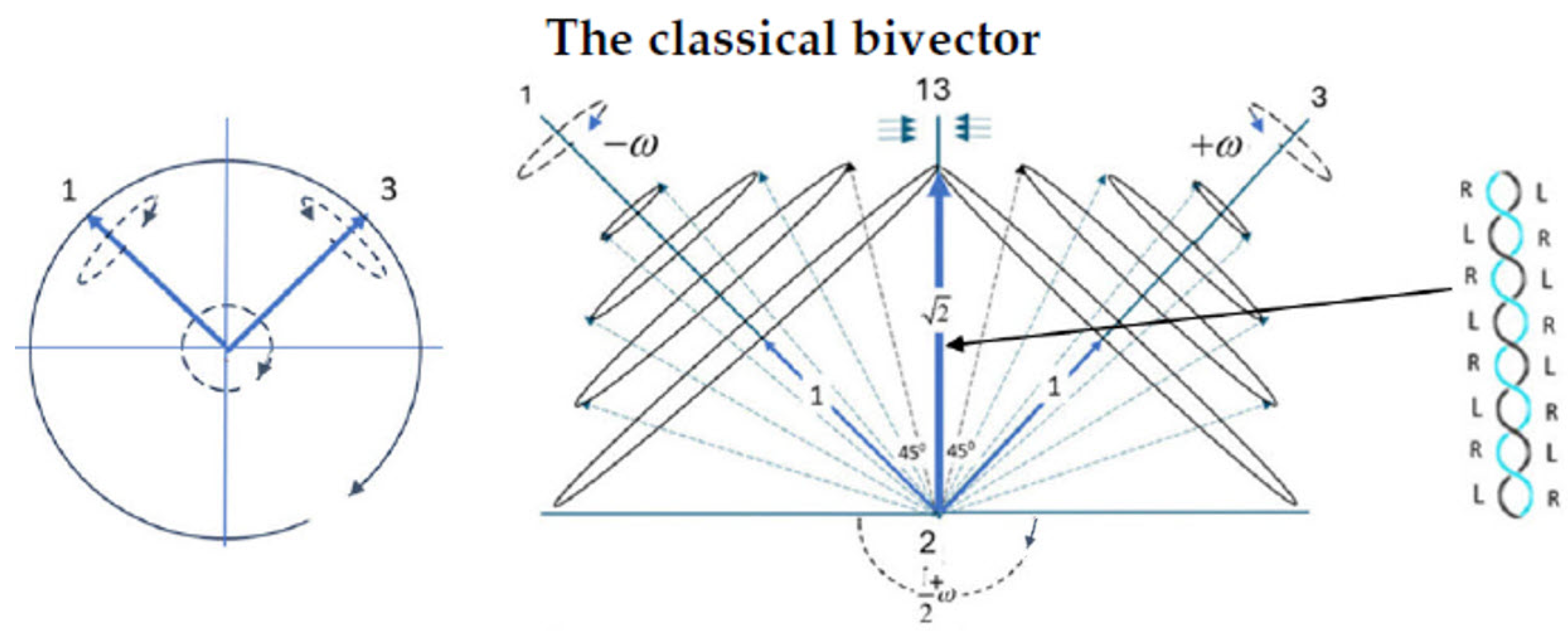
To visualize the motion, Figure 1 shows the bivector in the BFF as a classical structure defined by the blades $e_1$ and $e_3$, [8], rotating about the orthogonal axis $e_2$. This motion generates two cones of angular momentum, ${\mathbf{S}}_1$ and ${\mathbf{S}}_3$, which counter-precess at twice the frequency of the torque axis. The two blades have opposite chirality and form a mirror–symmetric pair about the bisector plane. Their coupled motion defines a continuous internal rotation that underlies the bivector structure.

Bivector spin is defined as the wedge product of the two angular momenta,

$$B={\mathbf{S}}_1\wedge {\mathbf{S}}_3,$$

(1)

thereby defining the interaction plane. Using solutions of Euler’s equations [2,9], the scalar and wedge products are

$$\begin{array}{cc}\hfill {\mathbf{S}}_1·{\mathbf{S}}_3& =cos\Phi \hfill \\ \hfill {\mathbf{S}}_1\wedge {\mathbf{S}}_3& =e_{2}sin\Phi ,\hfill \end{array}$$

(2)

where $\Phi$ is the angle between the two axes. The geometric product then gives

$$\begin{array}{cc}\hfill Q_B(\Phi )& ={\mathbf{S}}_1{\mathbf{S}}_3=cos\Phi +e_{2}sin\Phi \hfill \\ \hfill & =\exp (e_2\Phi ).\hfill \end{array}$$

(3)

This expresses the bivector dynamics by a rotor and therefore is a phase. It is carried by an electron and is transported through one slit or the other, but not both simultaneously.

As the angle $\Phi \to 0$, the system approaches a scalar limit corresponding to a symmetric double-helix state with even parity [2]. This defines the magnetic quantum state of $m=0$, which carries no external polarization or helicity. Here we assume that as spins propagate to the screen, no fields are present, and they do so in the $m=0$ state.

The Bivector Clock

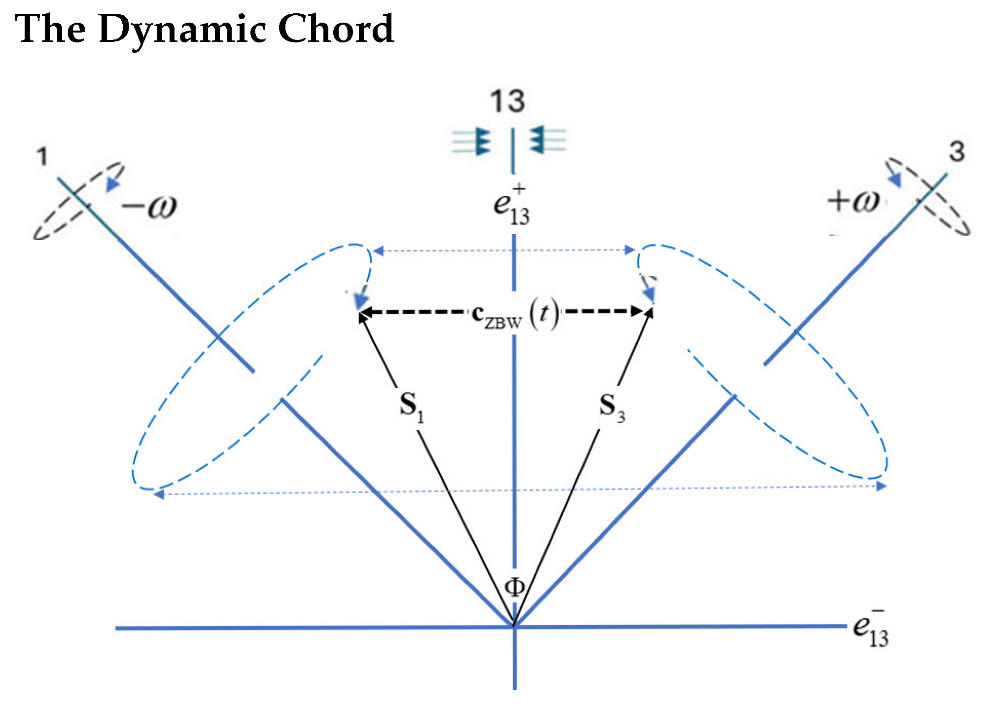
The counter-precessing blades generate a periodic internal motion. This is illustrated in Figure 2 as an oscillating chord, $c_{\mathrm{ZBW}}\left(\tau \right)$, between the tips of the two angular-momentum cones. The motion is parameterized by proper time $\tau$ and corresponds to the Zitterbewegung (ZBW) internal oscillation [10,11]. This periodic motion defines a natural internal phase and therefore an intrinsic clock carried by all electrons.

The phase relevant for the present work is associated with the rotor describing this internal motion, Equation (3). This accumulates from the slit plane to the detection screen. The two slits do not act as sources of waves and do not divide the electron into spatial components. Instead, for any given detection point, each slit defines a distinct geometrically admissible trajectory with a corresponding traversal time. Differences in traversal time lead directly to differences in accumulated clock phase. The second slit does not act dynamically on the electron; it serves only to define an alternative geometrically allowed path that enters the phase comparison at detection. In the conventional interpretation, the phase difference associated with the two channels is attributed to interference between matter-wave amplitudes. In the present formulation, the same phase relation arises from the transported internal clock phase carried by a localized electron. The two slits define distinct geometric traversal histories whose path-length difference,

$$\Delta s=s_1-s_2$$

(4)

determines the relative clock phase at the screen. The second slit therefore contributes geometrically through the definition of the phase-comparison term, rather than dynamically through self-interference.

In this way, the geometry of the apparatus fixes the path-length difference $\Delta s\left(y\right)$, which determines the proper-time difference $\Delta \tau \left(y\right)$, and hence the relative phase $\Delta \varphi \left(y\right)$ carried by the electron. The detection probability is therefore governed by this phase difference, establishing a deterministic mapping from geometry to phase from the traversal time.

3. The Clock as a Bivector Rotor

Let B denote the unit bivector generating this internal rotation, normalized such that

$$B^2=-1.$$

(5)

This rotation is generated by the Pauli bivector

$$B=i{\sigma }_2.$$

(6)

where the Pauli matrices are defined in the BFF, ${\sigma }_i$. The internal clock state is represented by the rotor [8]

$$R\left(\varphi \right)=\exp \left(-{\displaystyle \frac{1}{2}}\varphi i{\sigma }_2\right),$$

(7)

where $\varphi$ is the accumulated internal phase. Because the generator satisfies Equation (5), the exponential takes the trigonometric form

$$R\left(\varphi \right)=\cos \left({\displaystyle \frac{\varphi }{2}}\right)-i{\sigma }_2\sin \left({\displaystyle \frac{\varphi }{2}}\right).$$

(8)

The scalar projection of the rotor, ${\langle ·\rangle }_0$, isolates the phase-dependent amplitude,

$${\langle R\left(\varphi \right)\rangle }_0=\cos \left({\displaystyle \frac{\varphi }{2}}\right).$$

(9)

At this stage, the phase $\varphi$ is a purely internal BFF quantity. No wave number appears here, because the BFF contains no distinguished laboratory direction along which a spatial phase gradient can be defined. The rotor therefore represents a transported internal phase rather than a pre-existing wave in space.

The scalar projection has a direct correspondence with the standard trace operation in quantum mechanics, giving the scalar part of a multivector M,

$${\langle M\rangle }_0={\displaystyle \frac{1}{2}}\mathrm{Tr}\left(M\right),$$

(10)

While traces in the conventional formalism are associated with expectation values, the scalar projection, Equation (9), instead corresponds to the invariant part of a rotor and functions as an amplitude whose square yields the detection probability. The scalar projection therefore isolates the common phase associated with the rotor. The quantum-mechanical phase $\exp \left(i\varphi \right)$ and the bivector rotor phase $\exp (-B{\displaystyle \frac{\varphi }{2}})$ are mathematically equivalent. The difference is that the bivector phase has an explicit geometric interpretation as a rotation in a real plane, whereas the wavefunction phase is usually treated as an abstract complex quantity.

The two-slit apparatus produces different elapsed proper times along different geometric channels. The observable interference arises from the comparison of the corresponding internal rotor phases.

Channel Rotors and Relative Phase

The two geometric channels do not correspond to different bivector planes; both share the same internal generator B in their respective BFF descriptions. What differs between them is only the accumulated clock phase associated with the elapsed traversal time along each channel.

For a given channel $i\in \{1,2\}$ and screen coordinate y, let ${\tau }_i\left(y\right)$ denote the proper time accumulated by the internal clock. The corresponding phase is

$${\varphi }_i\left(y\right)={\omega }_C{\tau }_i\left(y\right)+{\varphi }_0,$$

(11)

where ${\omega }_C$ is the Compton clock frequency and ${\varphi }_0$ is a common source phase. The associated channel rotor is

$$R_i\left(y\right)=\exp \left(-{\displaystyle \frac{1}{2}}{\varphi }_i\left(y\right)B\right),i=1,2.$$

(12)

The physically relevant quantity is the relative rotor comparing the two channel clocks,

$$R_{12}\left(y\right)=R_1\left(y\right)R_2^{-1}\left(y\right)=\exp \left(-{\displaystyle \frac{1}{2}}\Delta \varphi \left(y\right)B\right),$$

(13)

where

$$\Delta \varphi \left(y\right)={\varphi }_1\left(y\right)-{\varphi }_2\left(y\right)={\omega }_C\left({\tau }_1\left(y\right)-{\tau }_2\left(y\right)\right)={\omega }_C\Delta \tau \left(y\right).$$

(14)

The relative rotor compares two phase histories of a single particle accumulated along distinct geometric channels, rather than two coexisting wave amplitudes.

Thus the relative phase is defined as the difference in accumulated proper time of the internal bivector clock, even though the two channels themselves are distinguished geometrically in the LFF. The observable interference amplitude is obtained from the scalar projection of the relative rotor,

$${〈R_{12}\left(y\right)〉}_0=cos\left({\displaystyle \frac{\Delta \varphi \left(y\right)}{2}}\right)=cos\left({\displaystyle \frac{{\omega }_C\Delta \tau \left(y\right)}{2}}\right),$$

(15)

up to the sign convention chosen for $\Delta \varphi$.

The remaining step is to relate the invariant clock phase difference $\Delta \varphi \left(y\right)$ to the geometry of the apparatus in the LFF. The two channels reaching the same screen coordinate y have a path-length difference

$$\Delta s\left(y\right)=s_1\left(y\right)-s_2\left(y\right),$$

(16)

defined entirely in the LFF. This geometric path difference determines the corresponding proper-time difference $\Delta \tau \left(y\right)$ and therefore the internal phase mismatch between the two channel rotors.

4. On Lorentz Transformations and Complementary Sectors

The purpose of this discussion is to clarify how the bivector clock phase is an internal geometric degree of freedom defined in the BFF, while the observable interference geometry is resolved in the LFF.

In conventional quantum mechanics, complementarity is associated with non-commuting observables, e.g., position and momentum. However, for spin, the usual statement that $S_x$ and $S_y$ are complementary is not precise. They are incompatible since the two cannot simultaneously exist as dispersion free states. However, both are superpositions of the same two dimensional Hilbert space, and so exist in a single algebraic sector.

In the bivector ontology developed here, spin possesses two structurally distinct sectors arising from parity decomposition and geometric splitting [2,5]. We therefore require a definition of complementarity specific to spin, reflecting domain structure rather than operator non-commutation.

More specifically, under the change in algebra from the Minkowski signature of the usual Dirac equation, $Cl(1,3)$, to that of the bivector, $Cl(2,2)$, space bifurcates [5] into a 2D disc, $Cl(1,2)$, in the BFF, and a quaternionic sector that spins the 13-plane in the LFF, residing on the $S^3$ hypersphere. These two sectors are distinct and complementary geometric structures. They are not related by Lorentz transformations, since one belongs to spacetime geometry while the other resides in an internal quaternionic space.

4.1. Complementarity of Spin

Contextuality of spin arises from the contrast between the isotropic internal rotation of the bivector plane and the anisotropic polarization that appears in a measurement field. In the bivector model, the free-flight electron in the $m=0$ state is isotropic and carries no externally defined polarization axis. The BFF describes the internal rotational dynamics of the bivector rotor, while the LFF describes polarization only after interaction with a measurement geometry or external field. The invariant quantity transported between them is the bivector clock phase, which remains a Lorentz scalar along the worldline. The BFF and the LFF therefore do not constitute two coordinate descriptions of a single spacetime related by a Lorentz transformation. Rather, they represent complementary geometric aspects of the bivector structure of spin: the BFF describes the internal rotational dynamics, while the LFF describes the externally instantiated polarization.

4.2. Phase Is a Scalar Invariant

The connection between the two descriptions is therefore not a frame transformation but a mapping along the particle worldline,

$$d\varphi ={\displaystyle \frac{1}{\mathit{ћ}}}{p}_{\mu }d{x}^{\mu },$$

(17)

which is a Lorentz scalar valid in all frames. Thus, the invariant phase provides a bridge between proper-time evolution and laboratory kinematics, where the measurable quantities emerge using coordinate time t in the LFF. Here, complementarity is geometric rather than canonical, arising from the parity-separated structure of the bivector rotor.

5. From Clock Phase to Spatial Phase

The internal bivector rotor introduced in Section 2 defines a periodic degree of freedom in the BFF. In the absence of external fields, this rotation is uniform in proper time, $\tau$, so that the accumulated phase is

$$d\varphi ={\omega }_{C}d\tau ={\displaystyle \frac{m{c}^2}{\mathit{ћ}}}d\tau ={\displaystyle \frac{1}{\mathit{ћ}}}{p}_{\mu }d{x}^{\mu }$$

(18)

where the Compton frequency follows from the Planck relation $E=\mathit{ћ}\omega$ for a free particle.

Since the phase is accumulated along the particle worldline, the appropriate quantity is the Lorentz-invariant scalar [12], formed from the four-momentum and spacetime displacement,

$$p^{\mu }=\left({\displaystyle \frac{E}{c}},\mathbf{p}\right),d{x}^{\mu }=(cdt,d\mathbf{x})$$

(19)

For free motion, using $p_{\mu }=m{u}_{\mu }$ with $u^{\mu }=d{x}^{\mu }/d\tau$, together with the invariant interval $d{x}_{\mu }d{x}^{\mu }=c^{2}d{\tau }^2$, one obtains

$$p_{\mu }d{x}^{\mu }=m{u}_{\mu }d{x}^{\mu }=m{c}^{2}d\tau$$

(20)

thereby recovering Equation (18). In the LFF, using the Minkowski signature, the invariant takes the form

$$p_{\mu }d{x}^{\mu }=Edt-\mathbf{p}·d\mathbf{x}=Edt-pds$$

(21)

For motion along the trajectory, where $d\mathbf{x}\Vert \mathbf{p}$, one has $\mathbf{p}·d\mathbf{x}=pds$, with $ds$ the differential path length. Combining these expressions gives

$$m{c}^{2}d\tau =Edt-pds$$

(22)

This is the relativistic action differential along the electron’s worldline. It expresses the proper-time clock phase in terms of laboratory energy and momentum, converting the internal proper-time evolution into a spatial phase along the trajectory. This equality follows because both expressions are generated by the same invariant action along the worldline, so the internal rotor phase is not analogous to, but identical with, the relativistic phase increment. The distinction of the present formulation is that the observed interference pattern is not derived from a superposition of extended wave amplitudes, but from a Lorentz-invariant phase carried by a localized particle.

Each electron produces a single localized detection event, with no memory or interaction between events, and the interference pattern emerges solely from the statistical accumulation of invariant phase differences. In this sense, the role traditionally attributed to the wavefunction is replaced by a geometric phase that is intrinsic, local, and consistent with relativistic invariance.

6. Fraunhofer Geometry and Path Difference

Integrating the invariant phase along a channel gives

$$\Delta \varphi ={\displaystyle \frac{1}{\mathit{ћ}}}\int (Edt-pds)$$

(23)

for each trajectory, $ds=vdt$, so the temporal and spatial contributions are not independent but combine to give the invariant proper–time phase, Equation (18). Each path therefore accumulates phase according to its own proper time, and the observable phase difference is obtained by comparing these phases at the same spacetime event.

The electron is prepared with a fixed energy E, which is the same for both channels. The temporal contributions are therefore common to both paths and cancel in the phase difference, Equation (23), leaving a spatial phase determined solely by the path-length difference. Up to a sign convention, this can be written as

$$\Delta \varphi ={\displaystyle \frac{p}{\mathit{ћ}}}\Delta s=k\Delta s$$

(24)

where k is the wave number. The wave number k is not introduced as an independent input, but is fixed by the invariant phase gradient derived below, so the simulation tests the event-level realization of this phase law rather than imposing it.

6.1. Double Slit Geometry

A detection event at screen position y corresponds to an observation angle $\phi$ relative to the normal to the slit plane. In the Fraunhofer regime $\left|\phi \right|\ll 1$,

$$tan\phi \simeq sin\phi \simeq \phi \simeq {\displaystyle \frac{y}{L}}$$

(25)

The geometric path-length difference between the two channels is then

$$\Delta s=dsin\phi \simeq {\displaystyle \frac{yd}{L}}$$

(26)

These are defined entirely in the LFF. The phase difference therefore becomes

$$\Delta \varphi \left(y\right)=k\Delta s\approx k{\displaystyle \frac{yd}{L}}$$

(27)

The observed fringe spacing thus reflects differences in accumulated proper time between the two paths, expressed in the laboratory frame as a geometric path difference. The wave number provides the conversion between the invariant proper–time phase and its spatial manifestation.

6.2. Detection Weight and Probability

We take the interference weight at coordinate y to be proportional to the scalar part of the relative rotor, Equation (15),

$$W\left(y\right)\propto {〈R_{12}\left(y\right)〉}_0$$

(28)

Its scalar projection represents the amplitude associated with the two geometric channel histories. Because the detection probability is proportional to the square of this projection, the probability density becomes,

$$P\left(y\right)\propto W^2\left(y\right)={cos}^2\left(k{\displaystyle \frac{yd}{2L}}\right)$$

(29)

yielding a normalized intensity profile when integrated over the screen coordinates. Here, the scalar projection extracts the invariant overlap of the two rotor phases, which serves as the physically relevant amplitude; its square then gives the detection probability. The simulation does not derive the interference law; rather, it numerically samples detection events from the analytically derived clock-phase distribution to test whether the observed event-by-event build-up is reproduced.

This identification ensures that the detection rule follows from the geometric structure of the rotor rather than being introduced as an independent postulate.

7. de Broglie Wavelength

When the electron propagates in the laboratory frame, the invariant clock phase is expressed in spacetime through the phase function

$$\varphi (x,t)=\omega t-kxk={\displaystyle \frac{p}{\mathit{ћ}}},\omega ={\displaystyle \frac{E}{\mathit{ћ}}}$$

(30)

This form follows directly from the invariant phase Equation (18), and does not introduce an independent wave description. With time held fixed, a spatial translation by one de Broglie wavelength ${\lambda }_{dB}$ advances the phase by $2\pi$,

$$\Delta \varphi =\varphi (x+{\lambda }_{dB},t)-\varphi (x,t)=k{\lambda }_{dB}=2\pi$$

(31)

which gives

$${\lambda }_{dB}={\displaystyle \frac{2\pi }{k}}={\displaystyle \frac{h}{p}}$$

(32)

Thus k is the spatial phase gradient of the transported clock,

$$k={\displaystyle \frac{\Delta \varphi }{{\lambda }_{dB}}}\approx {\displaystyle \frac{\partial \varphi }{\partial x}}$$

(33)

It converts proper-time evolution into a phase accumulated per unit length along the trajectory. It provides the bridge between the internal clock and the spatial interference pattern.

For an electron of mass $m_e$ and velocity v, with momentum $p=\gamma m_{e}v$, the de Broglie wavelength is

$${\lambda }_{dB}={\displaystyle \frac{h}{\gamma m_{e}v}}$$

(34)

which can be written in terms of the Compton wavelength ${\lambda }_C=h/\left(m_{e}c\right)$ as

$${\lambda }_{dB}={\displaystyle \frac{c}{\gamma v}}{\lambda }_C$$

(35)

The de Broglie wavelength emerges as the spatial phase scale associated with transport of the internal rotor phase. The two wavelengths do not represent separate physical oscillations. Rather, the internal bivector clock evolves in proper time, while in the laboratory the same invariant phase is resolved into temporal and spatial components associated with the particle’s energy E and momentum p. This provides a geometrical origin for de Broglie matter-waves.

8. Event-by-Event Build-Up

Individual events are discrete and localized: each electron produces exactly one impact point y on the screen. No single detection event displays an interference pattern. The interference structure emerges only through the accumulation of many such events.

The probability density $P\left(y\right)$, Equation (29), follows from the scalar projection of the relative rotor, Equation (15), giving a clock-phase difference between the two geometric channels. It specifies the likelihood that a given internal clock phase, constrained by the geometry of the apparatus, produces a detection at coordinate y.

An event-by-event description may therefore be formulated as follows. For the nth electron a detection coordinate $y_n$ is drawn from the probability density $P\left(y\right)$,

$$y_n\sim P\left(y\right)n=1,\dots ,N_{\mathrm{tot}}.$$

(36)

Each event contributes a single localized hit, $y_n\in \mathbb{R}$, with no memory of previous detections. The accumulated detection pattern after $N_{\mathrm{tot}}$ electrons is represented by the empirical distribution

$$N\left(y\right)={\displaystyle \sum _{n=1}^{N_{\mathrm{tot}}}}\delta \left(y-y_n\right).$$

(37)

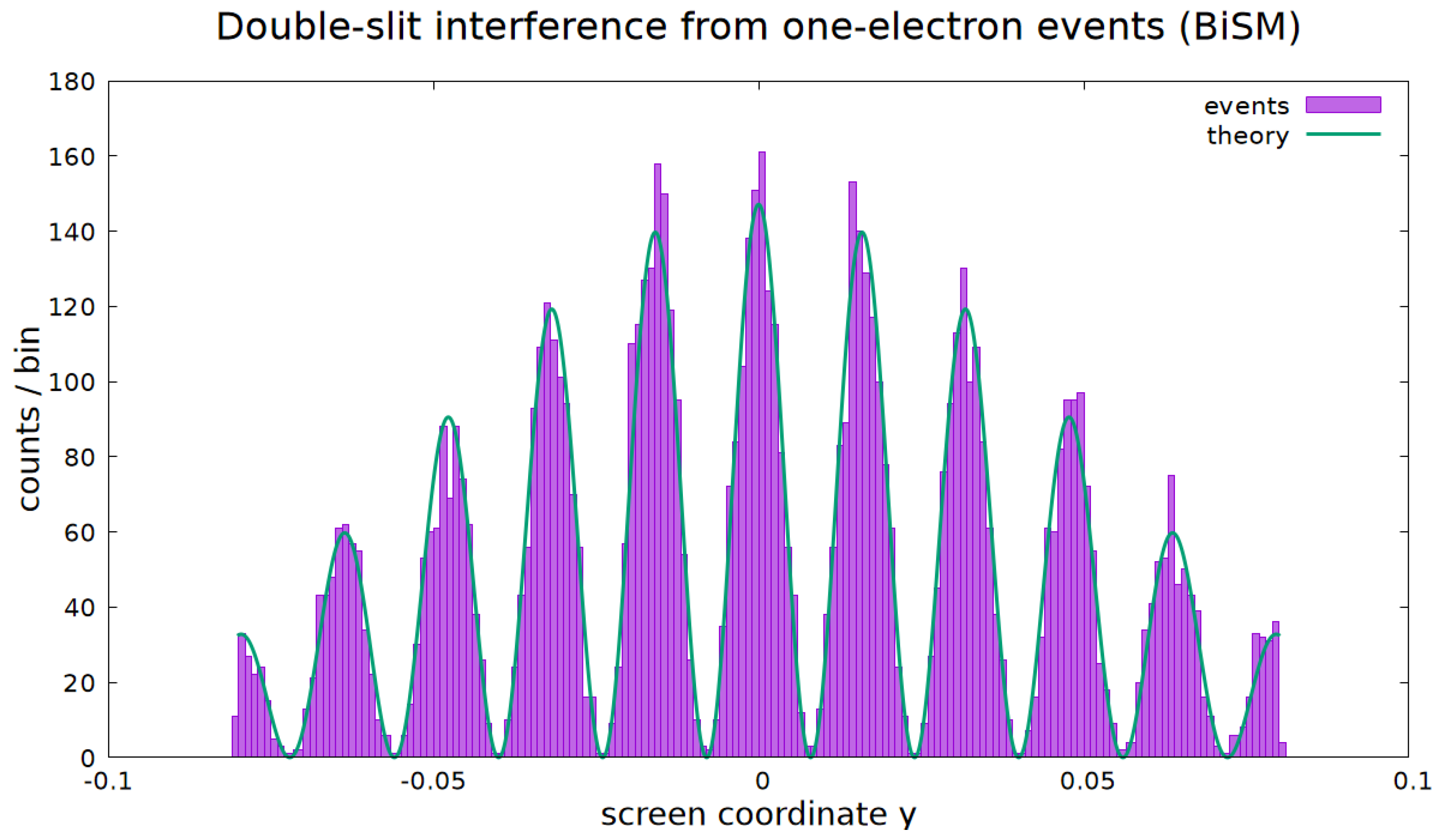
As the total number of events increases, the normalized histogram $N\left(y\right)/N_{\mathrm{tot}}$ converges to the smooth envelope defined by $P\left(y\right)$, Figure 3.

Lowering the source intensity reduces the rate at which events accumulate but does not alter the probability density $P\left(y\right)$. Consequently, the interference pattern persists unchanged in the one–electron–at–a–time limit. If one slit is closed, only a single clock history remains. In that case, the relative rotor reduces to unity; the interference weight becomes constant; and the detection distribution is governed solely by the single-slit geometry.

In the BiSM interpretation, which-way detection [1] destroys the coherence of the internal bivector clock by forcing local polarization and thereby breaking the phase relation between geometrically allowed paths. Once the bivector coherence is lost, the relative phase comparison responsible for the interference distribution can no longer occur, leaving only the classical sum of intensities.

The event–by–event build–up therefore provides a transparent account of single-electron interference. The observed pattern arises from the accumulation of localized detection events whose relative phase is fixed by the geometry of the apparatus.

8.1. Simulation of the Interference

The numerical procedure used to generate the event–by–event Double Slit interference pattern is based directly on the detection probability density derived from the rotor phase difference. For a detection coordinate y on the screen, the probability density is taken to be

$$P\left(y\right)\propto {cos}^2\left(k{\displaystyle \frac{yd}{2L}}\right){\mathrm{sinc}}^2\left(k{\displaystyle \frac{ya}{2L}}\right),$$

(38)

where a is the slit width. The cosine-squared factor arises from the scalar projection of the relative bivector rotor, giving a dependence on the phase difference $\Delta \varphi =k\Delta s$, while the ${\mathrm{sinc}}^2$ factor represents the standard single-slit diffraction envelope associated with the finite slit width.

Screen bins determine only histogram resolution. The geometric parameters of the apparatus are $N,L,d$ and a. The others are needed for the simulation. The two factors in Equation (38) are multiplicative as in Fraunhofer diffraction theory [3,4]. The simulation does not derive the pattern numerically; it tests whether event-wise sampling from the clock-phase distribution reproduces the observed build-up. The probability density is normalized numerically over the screen coordinate so that $\int P\left(y\right)dy=1$. No analytic normalization is assumed.

8.2. Event–by–Event Algorithm

Each event corresponds to a single electron detection. The sampling reflects the distribution generated by the internal clock phase differences between the two geometric channels.

• A trial emission angle $\varphi$ is sampled over the range $[-{\varphi }_{max},{\varphi }_{max}]$ by rejection sampling.
• For each trial angle, the detection weight is evaluated from the explicit two-channel geometry. The path lengths

  $$s_1=\sqrt{L^2+{(y-d/2)}^2},s_2=\sqrt{L^2+{(y+d/2)}^2}$$

  (39)

  with $y=Ltan\varphi$, determine the relative clock phase

  $$\Delta \varphi =k(s_1-s_2)$$

  (40)

  and hence the intensity follows the probability given by Equation (29).
• Once accepted, the event is assigned the screen coordinate

  $$y_n=Ltan{\varphi }_n$$

  (41)
• Each event contributes exactly one localized hit to the detection screen. There is no memory of previous events and no interaction between electrons.
• After N events, the accumulated pattern is represented as a histogram of counts per bin.
• For comparison with the event histogram, a smooth theory curve $P\left(y\right)$ is then evaluated on a uniform grid in y and normalized numerically.

Early stages of the accumulation appear noisy and structureless, while the familiar interference fringes emerge progressively as the number of events increases and statistical fluctuations diminish.

8.3. Reference Curve and Plot Construction

In Figure 3, the discrete histogram represents the simulated detection events. The smooth reference curve is obtained by evaluating the same analytic expression for $P\left(y\right)$ derived from the rotor phase difference on the screen grid, normalizing it numerically, and scaling it to counts per bin by multiplying by $N\Delta y$, where $\Delta y$ is the histogram bin width.

8.4. Approximations

Only standard and well-controlled approximations are employed:

• The far-field (Fraunhofer) approximation, $L\gg d,a$, allowing $sin\varphi \simeq y/L$.
• A well-defined longitudinal velocity v, so that geometric path-length differences correspond directly to clock time delays.
• A random initial internal phase at emission, reflecting lack of experimental control rather than intrinsic indeterminacy.
• Only the relative phase difference associated with a given screen coordinate enters the detection probability, so the observed fringe distribution is determined entirely by the geometrically defined path difference between the two admissible channels.

These approximations arise from the geometry of the apparatus and not from any assumption of wave propagation.

9. Fringe Spacings

The Double Slit experiment was first demonstrated by Thomas Young in 1802 in a celebrated presentation to the Royal Society [13,14]. His original work described the appearance of regularly spaced bright and dark bands, although numerical fringe spacings were not reported. He allowed sunlight to pass through a small aperture and then through two closely spaced slits, projecting the pattern onto a distant wall.

The fringe spacing is given by $\Delta y=\lambda L/d$, and for visible light ($\lambda \sim 5\times {10}^{-7}\mathrm{m}$), slit separations of order $d\sim {10}^{-4}\mathrm{m}$, and a screen distance $L\sim 1$–$2\mathrm{m}$, the fringe spacing becomes

$$\Delta y\sim {10}^{-3}\mathrm{m},$$

(42)

or about a millimeter, making the pattern directly visible.

In contrast, electron interference experiments involve wavelengths near ${10}^{-12}\mathrm{m}$, making the fringe spacing orders of magnitude smaller and requiring electron-optical magnification. For example, in Jönsson’s electron multi-slit experiment [15,16,17], electrons accelerated through 50 kV have a de Broglie wavelength of about $\lambda \approx 0.05$ Å. The slit spacing used for the two-slit geometry is approximately $d=2.0\mathrm{\mu }\mathrm{m}$, and the observation plane is located $L=0.35\mathrm{m}$ beyond the slits. These values imply a fringe spacing

$$\Delta y\approx {\displaystyle \frac{\lambda L}{d}}\approx 8.8\times {10}^{-7}\mathrm{m}$$

(43)

in reasonable agreement with the photographed diffraction pattern.

The simulation presented here uses scaled parameters that preserve the ratio $\lambda /d$, which determines the phase difference $\Delta \varphi =k\Delta s$, while expanding the pattern to a convenient numerical range through the choice of L. The parameters in

Table 1. Numerical parameters used in the event-by-event simulation producing the double-slit interference pattern. All values are taken directly from the Supplementary File double_slit.f90.

Parameter	Symbol	Value	Description
Number of events	N	8000	Total number of single-electron trials
Screen distance	L	$1.0$	Distance from slit plane to screen (arbitrary units)
Slit separation	d	$0.02$	Center-to-center slit separation
Slit width	a	$0.0025$	Slit width (controls envelope)
Angular range	${\varphi }_{max}$	$0.08$ rad	Maximum emission angle
Target fringes	$N_{\mathrm{fr}}$	10	Desired bright fringes across full range
Wavelength	$\lambda$	$3.19\times {10}^{-4}$	Effective de Broglie wavelength
Wave number	k	$1.97\times {10}^4$	Clock-phase gradient ($2\pi /\lambda$)
Slit amplitudes	$a_1,a_2$	$1.0,1.0$	Equal slit transmission
Histogram bins	$N_{\mathrm{bin}}$	2000	Screen bin resolution

therefore produce a fringe spacing of

$$\Delta y\approx 1.6\times {10}^{-2}$$

(44)

in the arbitrary screen units.

10. Conclusions

Hestenes [18] and Catillon [19] also discuss ZBW and a Compton clock in the context of fermions. The transported clock phase introduced here is similar in spirit to Feynman’s “stopwatch” phase [1], in that it accumulates along a path. However, in the present formulation, it represents a real internal dynamical variable of a single electron, rather than a computational phase assigned to multiple Feynman paths. Interestingly, de Broglie [20] also conceived of an internal clock, but did not resolve its frequency. Alternative realist descriptions of quantum phenomena have previously been proposed, notably Bohmian mechanics [21] and Nelson stochastic mechanics [22]. Bohmian mechanics retains a physically real guiding wave evolving in configuration space, while Nelson’s approach derives quantum behavior from an underlying stochastic process. The present formulation differs from both in that the physically relevant phase is attributed to an internal bivector rotor carried by a localized particle. No guiding wave or stochastic medium is introduced.

We have presented a formulation of single–electron double–slit interference in which the phase originates from a transported internal clock rather than from a spatially extended wave description. The internal bivector rotor defines a periodic degree of freedom in proper time, and differences in accumulated clock phase between geometric channels determine the detection statistics. The treatment is primarily classical, and the resulting interference pattern arises from geometric phase relations rather than from a quantum wave description.

The phase is a Lorentz-invariant scalar, allowing it to be expressed in both the BFF and LFF as a spatial gradient determined by the particle momentum. The de Broglie wavelength emerges as the spatial periodicity of this transported phase. This provides a direct and transparent account of single–event interference: an internal clock accumulates phase, and comparison of clock histories produces the observed pattern. The wave–like features arise from the spacetime representation of this phase. In the standard interpretation, the phase difference arises from interference between spatially extended matter waves, whereas in the bivector model it arises from comparison of transported internal clock phases carried by localized particles.

The existence of this internal clock depends on the bivector structure of spin. A point particle without internal structure cannot sustain such a clock. Interference therefore reflects internal dynamics and geometry. The presence of a deterministic internal timing mechanism suggests new ways to interpret and model quantum phenomena. These ideas might be considered speculative because the bivector approach was overlooked 100 years ago in favor of the matter–antimatter ontology. The bivector SM ontology is entirely different and not as well-tested as the SM. A relationship to spinors as fundamental, superposition, and chiral fields cannot be made, and they are replaced by real rotors that describe spin without superposition and without postulation.