A Discrete Version of Local Hausdorff Dimension on Infinite Fractal Networks

Abstract

In this paper, we define the local Hausdorff dimension on fractal networks inspired by the idea of $\alpha$-potential at a point $x\in {\mathbb{R}}^d$. We prove some basic properties of the local Hausdorff dimension and then obtain the local Hausdorff dimension of some networks. We also discuss a more generalized dimension definition, namely the subset Hausdorff dimension.

1. Introduction

The fractal property [1] was first proposed by Mandelbrot to measure the length of the coast of Britain. The length of the coast varies with different scale measurements and reaches infinity when the scale approaches 0. Mandelbrot found that a series of objects have the so-called Hausdorff dimension [2], which is not an integer. In previous research on fractals, various dimensions have been suggested, including box dimension [3], packing dimension [4], Assouad dimension [5], and quasi-Assouad dimension [6]. Very recently, Selmi et al. [7,8] discussed the general (multifractal) Hausdorff and packing dimensions of compact sets in Euclidean space and Borel probability measures by generalizing gauge dimension functions.

It is known that the Hausdorff dimension is hard to compute directly. Frostman’s significant conclusion [9] highlights the correlation between the Hausdorff dimension and potential; that is,

$${\dim }_H\left(E\right)=sup\left\{\alpha \ge 0:{\int }_{E\times E}{\displaystyle \frac{d\mu \left(x\right)d\mu \left(y\right)}{{|x-y|}^{\alpha }}}<\infty \right\},$$

(1)

where $\mu$ is a mass distribution supported on $E\subset {\mathbb{R}}^l$ (i.e., $\mu \left(E\right)=1$), and ${\dim }_H\left(E\right)$ is the Hausdorff dimension.

Throughout this paper, we consider simple, undirected, and connected graphs (networks). The fractal dimension of the network [10] is proposed to reveal the relationship between the minimum number of boxes needed to cover the network $N\left(l\right)$ and the box size l—that is, $N\left(l\right)\sim l^{-d}$, where d is the fractal dimension of the network. Considering different information in the box, such as the number of boxes, the number of nodes in each box, and the volume of each box, all box characteristics and box sizes follow the power law function, which induces different networks dimensions. Please refer to information dimension [11], correlation dimension [12], and volume dimension [13]. Some properties of complex networks, such as vulnerability and robustness, can be solved by various dimensions [14,15]. All the dimensions mentioned above are applied to illustrate the structural properties of the network at its scale. In addition, a network can be regarded as a discrete metric space, and its structure can be discussed by utilizing the dimensional properties on discrete metric spaces (see Refs. [16,17]). In terms of constructing fractals with given dimensions, Caldarola [18] introduced an infinite family of distinct d-dimensional Sierpiński tetrahedra.

Very recently, Zeng and Xi [19] provided a discrete version of the Hausdorff dimension of networks based on potential theory. Suppose that ${\{G_n=(V_n,E_n)\}}_{n\ge 0}$ is a family of networks, where $V_n$ and $E_n$ are the node set and the edge set of $G_n$, respectively. Let $d_n(u,v)$ be the metric between nodes u and v on $G_n$, and let

$$P_{\alpha }\left(G_n\right)={\displaystyle \frac{1}{{(\#V_n)}^2}}\sum _{{\displaystyle \genfrac{}{}{0pt}{}{u\ne v}{u,v\in V_n}}}{\displaystyle \frac{1}{{(d_n(u,v)/\mathrm{diam}\left(G_n\right))}^{\alpha }}}$$

be the $\alpha$-energy of $G_n$, where $\mathrm{diam}\left(G_n\right)={max}_{u,v\in V_n}{d}_n(u,v)$ is the diameter of $G_n$.

Definition 1.

For a sequence of networks $\{G_n=(V_n,E_n)\}$ with $\#V_n\to \infty$, the Hausdorff dimension ${\dim }_H\left(\left\{G_n\right\}\right)$ of $\left\{G_n\right\}$ is defined by

$${\dim }_H\left(\left\{G_n\right\}\right)=sup\left\{\alpha \ge 0:\underset{n\to \infty }{lim\; inf}{P}_{\alpha }\left(G_n\right)<\infty \right\}.$$

(2)

As far as we know, the earliest conception of local dimension originated from the mass dimension [16] and the density of fractals [20]. Let $B_v\left(r\right)=\{u:d(u,v)\le r\}$ be the ball of the central node v and radius r. A useful concept through which to investigate the local structure of a self-similar fractal F is the local dimension of its measure $\mu$ at v, which is given by

$${\dim }_{\mu }\left(v\right)=\underset{r\to 0}{lim}{\displaystyle \frac{\log \mu \left(B_v\left(r\right)\right)}{\log r}},$$

if the limit exists. The local dimension of sets has been applied in fractal geometry and information theory, as shown in [21,22]. Very recently, Achour and Selmi [23] have made fundamental contributions to the theory of generalized local Hausdorff dimension functions and local packing dimension functions in Euclidean space ${\mathbb{R}}^n$.

In recent decades, some dimensions focused on the central node of the network have been introduced. The local dimension $d_v$ of a network was proposed by Silva and Costa [24]. They found that $\#B_v\left(r\right)$ and $r^{d_v}$ are linearly positively correlated for some networks. Later, several additional local dimensions, such as fuzzy local dimension [25], local information dimension [26], and multi-local dimension [27], were studied for networks.

We intend to establish local dimensions without relying on coverings. Inspired by [19,20], we note that the $\alpha$-potential at a point $x\in {\mathbb{R}}^n$, resulting from the mass distribution $\mu$ on ${\mathbb{R}}^n$, is defined as

$${\varphi }_{\alpha }\left(x\right)=\int {\displaystyle \frac{d\mu \left(y\right)}{{|x-y|}^{\alpha }}}.$$

We provide a discrete version of the local Hausdorff dimension based on the $\alpha$-potential ${\varphi }_{\alpha }\left(x\right)$. We say a graph is local finite if every vertex has only finitely many vertices in its neighborhood of finite radius. Let $\tilde{G}=(\tilde{V},\tilde{E})$ be an infinite and local finite graph. Notice that $\mu$ is a mass distribution on fractals, and it can be discretized into a counting measure on $B_v\left(r\right)$; that is,

$$\mu \left(y\right)={\displaystyle \frac{1}{\#B_v\left(r\right)}}\mathrm{for}\mathrm{all}y\in B_v\left(r\right).$$

The continuous form of ${\varphi }_{\alpha }\left(x\right)$ contains no scale parameters and can be confined within a finite range. Hence, we introduce the radius r in the discrete form to implement the relative distance normalization via ${\displaystyle \frac{d(u,v)}{r}}$. Then the $\alpha$-potential at v of radius r in $\tilde{G}$ is naturally defined as

$$P_{\alpha }(v;r,\tilde{G})={\displaystyle \frac{1}{\#B_v\left(r\right)}}\sum _{{\displaystyle \genfrac{}{}{0pt}{}{u\ne v}{u\in B_v\left(r\right)}}}{\displaystyle \frac{1}{{(d(u,v)/r)}^{\alpha }}}.$$

Similar to the continuous version of Frostman’s lemma (see [20]), we expect that the dimension of the graph is no less than $\alpha$ whenever the $\alpha$-potential is finite. Accordingly, we present the following definition:

Definition 2.

For a node $v\in \tilde{V}$, we define the local Hausdorff dimension ${\dim }_H(v;\tilde{G})$ of node v as

$${\dim }_H(v;\tilde{G})=sup\left\{\alpha \ge 0:\underset{r\to \infty }{lim\; inf}{P}_{\alpha }(v;r,\tilde{G})<\infty \right\}.$$

The distance-based dimensions proposed in [19] and in the present paper also provide methodologies for investigating graph properties, such as the Harary index [28] and Harary energy [29].

The remainder of this paper is organized as follows: Section 2 contains some basic properties of the local Hausdorff dimension and the proof that the $\alpha$-Ahlfors regular networks possess the same local Hausdorff dimension. In Section 3, we provide a sum operation of two graphs and discuss changes in the local Hausdorff dimension under this operation. Section 4 investigates the local Hausdorff dimension of finite node sets. In the final section, we draw our conclusions.

2. Basic Properties and Results

In this section, we provide some basic notations. We use the notation $x\asymp y$ to indicate that there are positive constants $c_1$ and $c_2$ such that

$$c_{1}y\le x\le c_{2}y.$$

If only the left (right) side of the above inequality holds, then it is denoted as $y\succsim x$ ($y\precsim x$). Moreover, for two sequences $\left\{x_n\right\}$ and $\left\{y_n\right\}$, we use $\left\{x_n\right\}\asymp \left\{y_n\right\}$ to indicate that there exist positive constants $c_1$ and $c_2$ such that $c_1{y}_n\le x_n\le c_2{y}_n$ holds for all n. Let $S_k\left(v\right)=B_v\left(k\right)\setminus B_v(k-1)$ for $k\ge 1$. Thus, for $k\ge 1$, $\left\{S_k\left(v\right)\right\}$ is a sequence of disjoint spherical shells centred on the node v.

We now demonstrate that the local Hausdorff dimension is, in fact, dependent on the local structure of the base node v. The dimension calculations involve an upper estimate and a lower estimate, which will hopefully provide the same values.

The following statement can be easily obtained.

Proposition 1.

$P_{\alpha }(v;r,\tilde{G})$ are monotonically increasing in α.

Proposition 2.

If $\tilde{G}$ has a bounded diameter, then ${\dim }_H(v;\tilde{G})=0$ for any chosen node.

Proof. 

Suppose that $\mathrm{diam}\left(\tilde{G}\right)\le M$, $M>0$. We thus have

$$P_{\alpha }(v;r,\tilde{G})\ge {\displaystyle \frac{r^{\alpha }}{M^{\alpha }}}\to \infty$$

for any $\alpha >0$; this necessitates ${\dim }_H(v;\tilde{G})=0$. □

For two nodes near enough, they have the same dimension.

Proposition 3.

For two distinct nodes, $v_1$ and $v_2$, with $d(v_1,v_2)\le M$, where $M\in \mathbb{R}$, we have

$${\dim }_H(v_1;\tilde{G})={\dim }_H(v_2;\tilde{G}).$$

(3)

Proof. 

If $\mathrm{diam}\left(\tilde{G}\right)$ is bounded, then

$${\dim }_H(v_1;\tilde{G})={\dim }_H(v_2;\tilde{G})=0.$$

Now suppose that $\mathrm{diam}\left(G_n\right)\to \infty$ as $n\to \infty$. For $u\ne v_1$, $v_2$, and a large enough r, we have

$${\displaystyle \frac{1}{M+1}}{d}_n(u,v_2)\le d_n(u,v_1)\le (M+1)d_n(u,v_2).$$

Hence, the $\alpha$-potential of $v_1$ has lower and upper bounds; that is,

$${(M+1)}^{-\alpha }{P}_{\alpha }(v_2;r,\tilde{G})\le P_{\alpha }(v_1;r,\tilde{G})\le {(M+1)}^{\alpha }{P}_{\alpha }(v_2;r,\tilde{G}).$$

(4)

It is evident that ${\dim }_H(v_1;\tilde{G})\ge {\dim }_H(v_2;\tilde{G})$ by the right side of (4). Similarly, the left side of (4) yields ${\dim }_H(v_1;\tilde{G})\le {\dim }_H(v_2;\tilde{G})$. Therefore, ${\dim }_H(v_1;\tilde{G})={\dim }_H(v_2;\tilde{G})$. □

We say that $\tilde{G}$ is $\alpha$-Ahlfors regular at node v if there are positive constants $c_1$ and $c_2$ such that

$$c_1{r}^{\alpha }\le \#(\tilde{V}\cap B_v\left(r\right))\le c_2{r}^{\alpha }$$

(5)

for all reasonable $1\le r$. If (5) holds for all $v\in \tilde{G}$, we then say $\tilde{G}$ is $\alpha$-Ahlfors regular.

Lemma 1.

$\tilde{G}$ is α-Alhfors regular at v if there are positive constants $c_1$ and $c_2$ such that $c_1{\theta }^{k\alpha }\le \#(\tilde{V}\cap B_v\left({\theta }^k\right))\le c_2{\theta }^{k\alpha }$ for some $\theta >1$ and all k are large enough.

Proof. 

For $1\le r$, there exists a constant k such that ${\theta }^{k-1}\le r\le {\theta }^k$. Then

$$\#(V\cap B_v\left(r\right))\le \#(V\cap B_v\left({\theta }^k\right))\le c_2{\theta }^{k\alpha }\le c_2{\theta }^{\alpha }{r}^{\alpha }$$

and

$$\#(V\cap B_v\left(r\right))\ge \#(V\cap B_v\left({\theta }^{k-1}\right))\ge c_2{\theta }^{(k-1)\alpha }\ge c_1{\theta }^{-\alpha }{r}^{\alpha }.$$

Hence,

$$c_1{\theta }^{-\alpha }{r}^{\alpha }\le \#(V\cap B_v\left(r\right))\le c_2{\theta }^{\alpha }{r}^{\alpha }.$$

We now see that $\tilde{G}$ is $\alpha$-Ahlfors regular at v. □

The following lemma provides an effective method to approximate the potential of a node in networks.

Lemma 2.

For $0\le \alpha <d$, we have

$${\displaystyle \sum _{k=1}^n}{\left({\displaystyle \frac{1}{k}}\right)}^{\alpha }(k^d-{(k-1)}^d)\asymp {\displaystyle \frac{d}{d-\alpha }}{n}^{d-\alpha }.$$

Proof. 

To show ${\{k^d-{(k-1)}^d\}}_k\asymp {\left\{d{k}^{d-1}\right\}}_k$, it is equivalent to prove that

$$F\left(x\right)={\displaystyle \frac{x^d-{(x-1)}^d}{x^{d-1}}}=x\left(1-{\left(1-{\displaystyle \frac{1}{x}}\right)}^d\right)$$

has a positive lower bound and a finite upper bound for all $x\ge 2$.

Using the Bernoulli inequality, one has

$$F\left(x\right)\le x\left(1-{\left(1-{\displaystyle \frac{1}{x}}\right)}^{d+1}\right)\le x\left(1-\left(1-{\displaystyle \frac{d+1}{x}}\right)\right)=d+1.$$

Similarly, one has

$$F\left(x\right)\ge x\left(1-{\left(1-{\displaystyle \frac{1}{x}}\right)}^1\right)=1,$$

for $d\ge 1$, and

$$F\left(x\right)\ge x\left(1-\left(1-{\displaystyle \frac{d}{x}}\right)\right)=d,$$

for $d\in (0,1)$. It follows that $F\left(x\right)\in [min\{d,1\},d+1]$.

Hence,

$${\displaystyle \sum _{k=1}^n}{\left({\displaystyle \frac{1}{k}}\right)}^{\alpha }(k^d-{(k-1)}^d)\asymp {\displaystyle \sum _{k=1}^n}d{k}^{d-\alpha -1}.$$

Since

$$\underset{n\to \infty }{lim}{\displaystyle \frac{1}{n}}{\displaystyle \sum _{k=1}^n}{\left({\displaystyle \frac{k}{n}}\right)}^{d-\alpha -1}={\int }_0^1{x}^{d-\alpha -1}\mathrm{d}x={\displaystyle \frac{1}{d-\alpha }},$$

it follows that

$${\displaystyle \sum _{k=1}^n}{\left({\displaystyle \frac{1}{k}}\right)}^{\alpha }(k^d-{(k-1)}^d)\asymp {\displaystyle \frac{d}{d-\alpha }}{n}^{d-\alpha },$$

as desired. □

Theorem 1.

If $\tilde{G}$ is d-Ahlfors regular at v, then ${\dim }_H(v;\tilde{G})=d$.

Proof. 

We see that $\#B_v\left(r\right)\asymp r^d$ since $\tilde{G}$ is Ahlfors regular at v. We obtain

$$P_{\alpha }(v;r,\tilde{G})={\displaystyle \frac{1}{\#B_v\left(r\right)}}{\displaystyle \sum _{k=1}^r}\sum _{u\in S_v\left(k\right)}{\left({\displaystyle \frac{r}{k}}\right)}^{\alpha }\asymp {\displaystyle \frac{1}{r^d}}{\displaystyle \sum _{k=1}^r}\sum _{u\in S_v\left(k\right)}{\left({\displaystyle \frac{r}{k}}\right)}^{\alpha }.$$

(6)

We first show that ${\dim }_H\left(\tilde{G}\right)\le d$. If $\alpha >d$, we then have $P_{\alpha }(v;r,G_n)\succsim r^{\alpha -d}\to \infty$ by taking only the term $k=1$ in the sum of (6). Thus, ${\dim }_H(v;\tilde{G})\le d$.

Now assume that $\alpha <d$. We need an appropriate upper bound for $P_{\alpha }(v;r,\tilde{G})$. It follows from (6) that

$$P_{\alpha }(v;r,\tilde{G})\asymp {\displaystyle \frac{1}{r^{d-\alpha }}}{\displaystyle \sum _{k=1}^r}{\left({\displaystyle \frac{1}{k}}\right)}^{\alpha }\#S_v\left(k\right).$$

Recall that $\tilde{G}$ is d-Ahlfors regular at v. It follows that

$${\displaystyle \sum _{k=1}^t}\#S_v\left(k\right)\le c_2{t}^d,t=1,2,\dots r.$$

Since $\left\{{\left({\displaystyle \frac{1}{k}}\right)}^{\alpha }\right\}$ is a monotonically decreasing sequence, $\#S_v\left(k\right)$ attains higher priority in value assignment for smaller indices k. We may set $\#S_v\left(k\right)=c_2(k^d-{(k-1)}^d)$ for $k\in \{1,2,\dots ,r\}$ to maximize ${\sum }_{k=1}^r{\left({\displaystyle \frac{1}{k}}\right)}^{\alpha }\#S_v\left(k\right)$ and thereby obtain

$${\displaystyle \sum _{k=1}^r}{\left({\displaystyle \frac{1}{k}}\right)}^{\alpha }\#S_v\left(k\right)\le {\displaystyle \sum _{k=1}^r}{\left({\displaystyle \frac{1}{k}}\right)}^{\alpha }{c}_2\left(k^d-{(k-1)}^d\right).$$

(7)

Then, using Lemma 2, we deduce that

$$\begin{array}{cc}\hfill P_{\alpha }(v;r,\tilde{G})& \precsim r^{\alpha -d}{\displaystyle \sum _{k=1}^r}{\left({\displaystyle \frac{1}{k}}\right)}^{\alpha }{c}_2\left(k^d-{(k-1)}^d\right)\hfill \\ & \asymp r^{\alpha -d}{\displaystyle \frac{d}{d-\alpha }}{r}^{d-\alpha }<\infty .\hfill \end{array}$$

It follows that ${\dim }_H(v;\tilde{G})\ge d$. Combining all the above discussions, we conclude that ${\dim }_H(v;\tilde{G})=d$. □

Corollary 1.

If there exists a $\theta >1$ such that $\#(V\cap B_v\left({\theta }^k\right))\asymp m^k$ for all $k\ge 1$, then

$${\dim }_H(v;\tilde{G})={\displaystyle \frac{\log m}{\log \theta }}.$$

Proof. 

Notice that $m={\theta }^{\log m/\log \theta }$. Then using Theorem 1, we obtain the conclusion. □

We say that $\left\{G_n\right\}$ is $\alpha$-Ahlfors regular if there are positive constants $c_1$ and $c_2$ such that, for all $v\in G_n$, $c_1{r}^{\alpha }\le \#(V_n\cap B_v\left(r\right))\le c_2{r}^{\alpha }$, where $1\le r\le \mathrm{diam}\left(G_n\right)$.

Theorem 2.

If $\left\{G_n\right\}$ is d-Ahlfors regular, then ${\dim }_H\left(\left\{G_n\right\}\right)=d$.

Proof. 

The condition ${\left(\mathrm{diam}\left(G_n\right)\right)}^d\asymp \#V_n\to \infty$ implies $\mathrm{diam}\left(G_n\right)\to \infty$.

Suppose that $\alpha <d$. By an argument similar to that for Equation (7) and using Lemma 2, we can deduce that

$$\begin{array}{cc}\hfill P_{\alpha }\left(G_n\right)& \asymp {\displaystyle \frac{1}{{\left(\mathrm{diam}\left(G_n\right)\right)}^{2d}}}\sum _{u\in V_n}\sum _{{\displaystyle \genfrac{}{}{0pt}{}{v\ne u}{v\in V_n}}}{\left({\displaystyle \frac{\mathrm{diam}\left(G_n\right)}{d_n(u,v)}}\right)}^{\alpha }\hfill \\ \hfill & ={\displaystyle \frac{1}{{\left(\mathrm{diam}\left(G_n\right)\right)}^{2d-\alpha }}}\sum _{u\in V_n}{\displaystyle \sum _{r=1}^{\mathrm{diam}\left(G_n\right)}}\sum _{v\in S_u\left(r\right)}{\left({\displaystyle \frac{1}{r}}\right)}^{\alpha }\hfill \\ \hfill & \le {\displaystyle \frac{1}{{\left(\mathrm{diam}\left(G_n\right)\right)}^{2d-\alpha }}}\sum _{u\in V_n}{\displaystyle \sum _{r=1}^{\mathrm{diam}\left(G_n\right)}}{\left({\displaystyle \frac{1}{r}}\right)}^{\alpha }{c}_2(r^d-{(r-1)}^d)\hfill \\ \hfill & \asymp {\displaystyle \frac{1}{{\left(\mathrm{diam}\left(G_n\right)\right)}^{2d-\alpha }}}\sum _{u\in V_n}{\displaystyle \frac{d}{d-\alpha }}{\left(\mathrm{diam}\left(G_n\right)\right)}^{d-\alpha }\hfill \\ \hfill & \asymp {\displaystyle \frac{d}{d-\alpha }}<\infty ,\hfill \end{array}$$

which implies ${\dim }_H\left(\left\{G_n\right\}\right)\ge d$.

Now assume that $d<\alpha$. We have

$$\begin{array}{cc}\hfill P_{\alpha }\left(G_n\right)& \asymp {\displaystyle \frac{1}{{\left(\mathrm{diam}\left(G_n\right)\right)}^{2d}}}\sum _{u\in V_n}\sum _{{\displaystyle \genfrac{}{}{0pt}{}{v\ne u}{v\in V_n}}}{\left({\displaystyle \frac{\mathrm{diam}\left(G_n\right)}{d_n(u,v)}}\right)}^{\alpha }\hfill \\ \hfill & \ge {\displaystyle \frac{1}{{\left(\mathrm{diam}\left(G_n\right)\right)}^{2d}}}\sum _{u\in V_n}\sum _{{\displaystyle \genfrac{}{}{0pt}{}{v\ne u}{v\in V_n\cap S_u\left(1\right)}}}{\left({\displaystyle \frac{\mathrm{diam}\left(G_n\right)}{1}}\right)}^{\alpha }\hfill \\ \hfill & \ge {\left(\mathrm{diam}\left(G_n\right)\right)}^{\alpha -d}\to \infty .\hfill \end{array}$$

It follows that ${\dim }_H\left(\left\{G_n\right\}\right)\le d$, and the conclusion is complete. □

Example 1

(Lattice in ${\mathbb{Z}}^d$). Define the cubical lattice graph $L_n$ by node set ${[-n,n]}^d\cap {\mathbb{Z}}^d$ and edge set $\{u\sim v:\parallel u-v{\parallel }_1=1\}$. Consider the local Hausdorff dimension of $\tilde{L}=\underset{n\to \infty }{lim}{L}_n$ at origin O. Because of d-Ahlfors regularity of $\tilde{L}$, one has ${\dim }_H(O;\tilde{L})=d$ and ${\dim }_H\left(\left\{G_n\right\}\right)=d$.

Example 2.

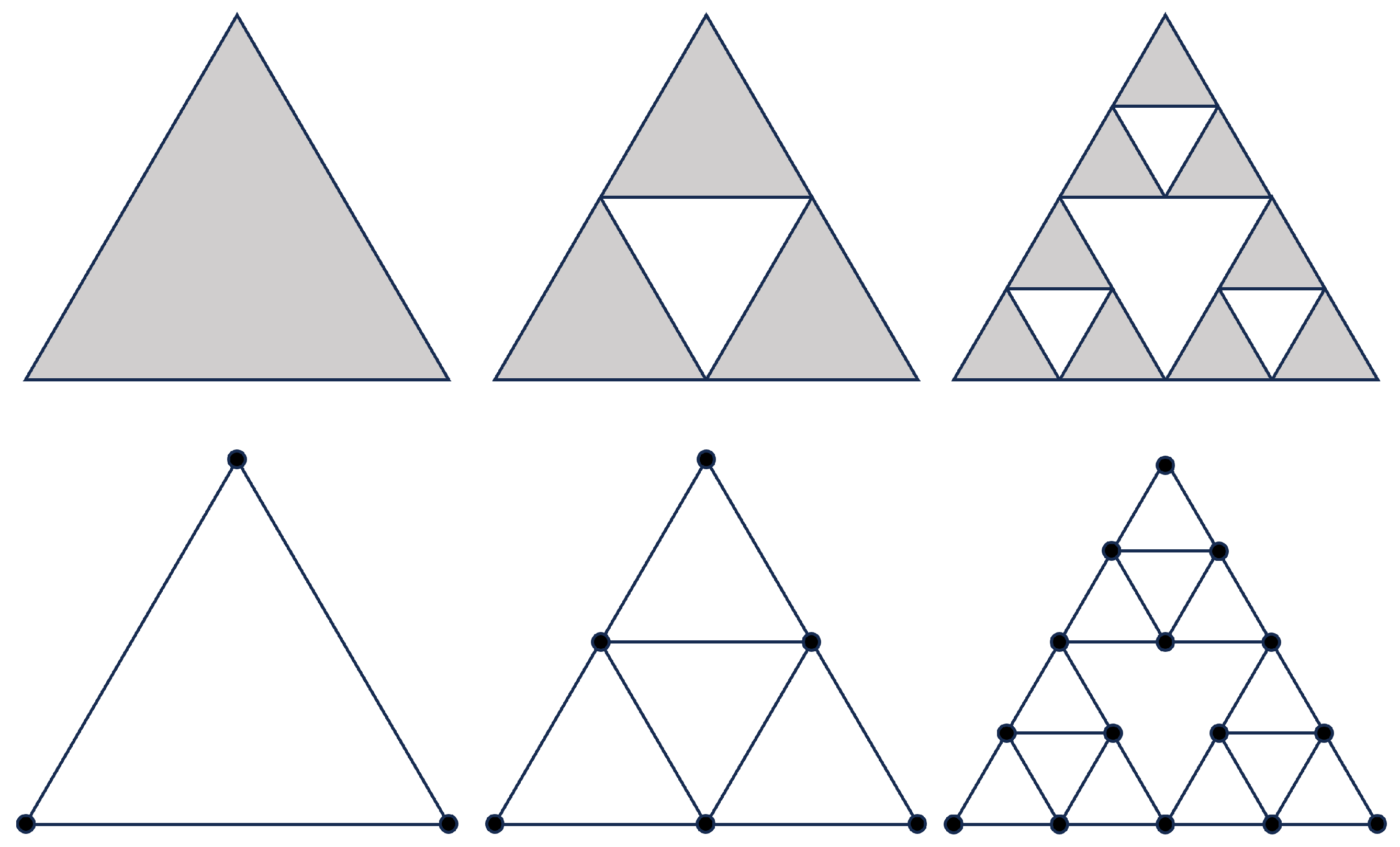
For the skeleton networks $S{T}_{\infty }=\underset{n\to \infty }{lim}S{T}_n$ induced by the d-dimensional Sierpiński tetrahedron (see Figure 1 for the Sierpiński gasket as the 2-dimensional case), we check Ahlfors regularity of $S{T}_{\infty }$ via Lemma 1. Taking $\theta =2$, $B_v\left(2^k\right)$ covers finite copies of $S{T}_k$ in $S{T}_{\infty }$. Hence, $\#(V\left(S{T}_{\infty }\right)\cap B_v\left(2^k\right))\asymp \#V_k\asymp {(d+1)}^k$. It is now clear that ${\dim }_H\left(\left\{S{T}_n\right\}\right)={\dim }_H(v;S{T}_{\infty })=\log (d+1)/\log 2$.

We now give a planar network family which may have no less than dimension 2.

Example 3.

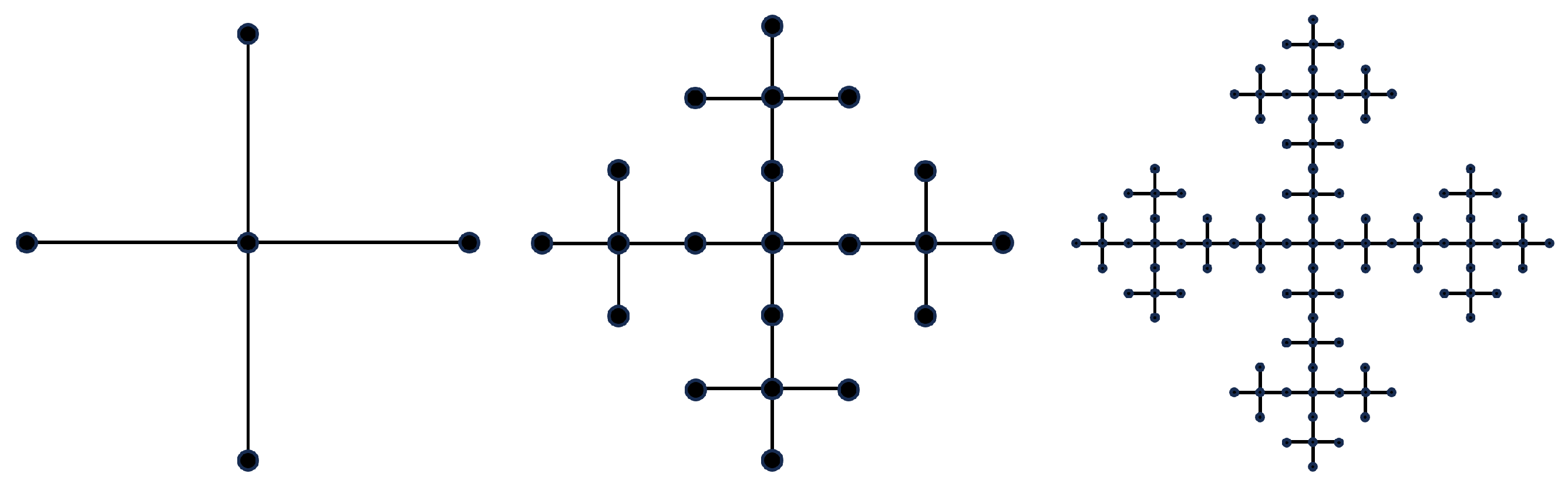
Let $K_{1,m}$ be a star graph, where $m\in \mathbb{N}$. We start with initial graph $G_1=K_{1,2^m}$ and construct $G_n$ by attaching a copy of $G_{n-1}$ to each branch of $G_{n-1}$ through the single node summation at the diametrical node. We set $\tilde{G}=\underset{n\to \infty }{lim}{G}_n$. See Figure 2 for Vicsek fractal with initial graph $K_{1,4}$. A similar argument to Example 2 shows that if $\theta =3$, then $\#(V\cap B_v\left(3^k\right))\asymp {(2^m+1)}^k$ for $v\in V$. Thus,

$${\dim }_H\left(\left\{G_n\right\}\right)={\dim }_H(v;\tilde{G})={\displaystyle \frac{\log (2^m+1)}{\log 3}}.$$

It is evident that ${\dim }_H(v;\tilde{G})\ge 2$ if $m\ge 3$. One of the reasons is that for $n\in \mathbb{N}$, despite $G_n$ being a planar graph, it can be embedded in the lattice graph of ${\mathbb{Z}}^m$.

We give an example of a heterogeneous graph below.

Example 4.

Given a root node v, a tree $\tilde{T}$ can be constructed by the following rules:

(1) 

Node u has two children if $d(u,v)=m^k-1$, $k=0,1,2,\dots$;

(2) 

Node u has only one child if $d(u,v)\ne m^k-1$.

For $m^k\le r<m^{k+1}-1$, we have ${\sum }_{i=1}^k{\left(2m\right)}^i\le \#B_v\left(r\right)<{\sum }_{i=1}^{k+1}{\left(2m\right)}^i$, which implies $\#B_v\left(r\right)\asymp {\sum }_{i=1}^k{\left(2m\right)}^i\asymp {\left(2m\right)}^k$. It is immediately evident that

$$\begin{array}{cc}\hfill P_{\alpha }(v;r,\tilde{T})& \asymp {\displaystyle \frac{1}{{\left(2m\right)}^k}}{\displaystyle \sum _{i=1}^r}{\left({\displaystyle \frac{r}{i}}\right)}^{\alpha }\#S_v\left(i\right)\hfill \\ \hfill & \asymp {\displaystyle \frac{1}{{\left(2m\right)}^k}}{\displaystyle \sum _{i=0}^k}{\displaystyle \sum _{j=m^i}^{m^{i+1}-1}}{\left({\displaystyle \frac{r}{j}}\right)}^{\alpha }\#S_v\left(j\right)\hfill \\ \hfill & \asymp {\displaystyle \frac{1}{{\left(2m\right)}^k}}{\displaystyle \sum _{i=1}^k}{\left({\displaystyle \frac{m^k}{m^i}}\right)}^{\alpha }{\left(2m\right)}^i\hfill \\ \hfill & =\left\{\begin{array}{cc}k,\hfill & \mathrm{if}\alpha ={\displaystyle \frac{\log 2m}{\log m}},\hfill \\ 2m{\displaystyle \frac{1-\frac{m^{k\alpha }}{{\left(2m\right)}^k}}{2m-m^{\alpha }}},\hfill & \mathrm{if}\alpha \ne {\displaystyle \frac{\log 2m}{\log m}}.\hfill \end{array}\right.\hfill \end{array}$$

Hence, as r tends to ∞, we have $\underset{r\to \infty }{lim}{P}_{\alpha }(v;r,\tilde{T})\asymp {\displaystyle \frac{2m}{2m-m^{\alpha }}}<\infty$ for $\alpha <{\displaystyle \frac{\log 2m}{\log m}}$, while $P_{\alpha }(v;r,\tilde{T})\to \infty$ for $\alpha \ge {\displaystyle \frac{\log 2m}{\log m}}$. We obtain ${\dim }_H(v;\tilde{T})={\displaystyle \frac{\log 2m}{\log m}}$.

It follows from Corollary 1 that the fractal dimension increases when the growth rate of the nodes is much faster than that of the network scale. Furthermore, we obtain the following theorem.

Theorem 3.

If there exists a constant $\lambda >1$ such that $\#B_v\left(r\right)\asymp {\lambda }^r$ for $r\in {\mathbb{Z}}_{+}$, then ${\dim }_H(v;\tilde{G})=\infty$.

Proof. 

We need to verify that $P_{\alpha }(v;r,\tilde{G})$ is bounded. By directly estimating the shell cardinalities, we have $\#S_v\left(k\right)\le c_2{\lambda }^k-c_1{\lambda }^{k-1}\le c_2{\lambda }^k$ for $c_2\ge c_1>0$ and $k\in \{1,2,\dots ,r\}$. Hence

$$\begin{array}{cc}\hfill P_{\alpha }(v;r,\tilde{G})& ={\displaystyle \frac{1}{\#B_v\left(r\right)}}{\displaystyle \sum _{k=1}^r}\sum _{u\in S_v\left(k\right)}{\left({\displaystyle \frac{r}{k}}\right)}^{\alpha }\hfill \\ \hfill & \precsim {\displaystyle \frac{1}{{\lambda }^r}}{\displaystyle \sum _{k=1}^r}{\left({\displaystyle \frac{r}{k}}\right)}^{\alpha }{\lambda }^k\hfill \\ \hfill & ={\displaystyle \frac{1}{{\lambda }^r}}{\displaystyle \sum _{k=1}^{\left[r/2\right]}}{\left({\displaystyle \frac{r}{k}}\right)}^{\alpha }{\lambda }^k+{\displaystyle \frac{1}{{\lambda }^r}}{\displaystyle \sum _{k=\left[r/2\right]+1}^r}{\left({\displaystyle \frac{r}{k}}\right)}^{\alpha }{\lambda }^k\hfill \\ \hfill & \le {\displaystyle \frac{r^{\alpha }}{{\lambda }^r}}{\displaystyle \sum _{k=1}^{\left[r/2\right]}}{\lambda }^k+{\displaystyle \frac{2^{\alpha }}{{\lambda }^r}}{\displaystyle \sum _{k=\left[r/2\right]+1}^r}{\lambda }^k\hfill \\ \hfill & <\infty ,\hfill \end{array}$$

for any given $\alpha >0$. The last inequality in the above formula holds since, as $r\to \infty$, $0<{\displaystyle \frac{r^{\alpha }}{{\lambda }^r}}{\sum }_{k=1}^{\left[r/2\right]}{\lambda }^k<{\displaystyle \frac{r^{\alpha }{\lambda }^{\left[r/2\right]+1}}{(\lambda -1){\lambda }^r}}\to 0$ and $0<{\displaystyle \frac{2^{\alpha }}{{\lambda }^r}}{\sum }_{k=\left[r/2\right]+1}^r{\lambda }^k<{\displaystyle \frac{2^{\alpha }}{{\lambda }^r}}·{\displaystyle \frac{{\lambda }^{r+1}}{\lambda -1}}={\displaystyle \frac{2^{\alpha }\lambda }{\lambda -1}}<\infty$ for any given $\alpha >0$. It follows that ${\dim }_H(v;\tilde{G})=\infty$. □

Example 5.

The binary tree is a tree with node set ${\{a,b\}}^{\mathbb{N}}=\{\mathsf{\varnothing },a,b,aa,ab,ba,bb,\dots \}$ and edge set $\{u\sim v:v=ua\mathit{or}ub\}$. The Fibonacci tree $\tilde{F}$ is a node-induced subtree of a binary tree with node set $\{v=v_1{v}_2\cdots v_m\in {\{a,b\}}^{\mathbb{N}}:v_i{v}_{i+1}\ne bb\mathit{for}\mathit{all}i\}$. Using the analytical expression of the Fibonacci sequence, we obtain $\#B_v\left(r\right)\asymp {\phi }^r$, where $\phi ={\displaystyle \frac{1+\sqrt{5}}{2}}>1$ and v is a node in $\tilde{F}$. By Theorem 3, it is plain that ${\dim }_H(v;\tilde{F})=\infty$.

From the definition of $d_v$, $\#B_v\left(r\right)\asymp r^{d_v}$, we see that the local dimension of $v\in \tilde{G}$ is $d_v$ if and only if $\tilde{G}$ is $d_v$-Ahlfors regular at v. For general graphs, define the upper and lower local dimensions by

$${\overline{d}}_v=\underset{r\to \infty }{\overline{lim}}{\displaystyle \frac{\log \#B_v\left(r\right)}{\log r}}\mathrm{and}{\underline{d}}_v=\underset{r\to \infty }{\underline{lim}}{\displaystyle \frac{\log \#B_v\left(r\right)}{\log r}},$$

respectively.

Theorem 4.

We have ${\dim }_H(v;\tilde{G})\le {\overline{d}}_v$.

Proof. 

For a bounded-diameter graph $\tilde{G}$, ${\dim }_H(v;\tilde{G})=0\le {\overline{d}}_v$. Now assume that $\mathrm{diam}\left(\tilde{G}\right)=\infty$. It is sufficient to show

$$\underset{r\to \infty }{lim}{\displaystyle \frac{1}{\#B_v\left(r\right)}}\sum _{u\in B_v\left(r\right)}{\left({\displaystyle \frac{r}{d(u,v)}}\right)}^{\alpha }=\infty \mathrm{for}\mathrm{any}\alpha >{\overline{d}}_v.$$

Note that $c\#B_v\left(r\right)\le r^{{\overline{d}}_v+\epsilon }$ for a constant $c>0$ and $\epsilon \in (0,\alpha -{\overline{d}}_v)$. We thus obtain

$$\begin{array}{cc}\hfill {\displaystyle \frac{1}{\#B_v\left(r\right)}}\sum _{u\in B_v\left(r\right)}{\left({\displaystyle \frac{r}{d(u,v)}}\right)}^{\alpha }& ={\displaystyle \frac{r^{\alpha -{\overline{d}}_v-\epsilon }}{\#B_v\left(r\right)}}\sum _{u\in B_v\left(r\right)}{\left({\displaystyle \frac{1}{d(u,v)}}\right)}^{\alpha }{r}^{{\overline{d}}_v+\epsilon }\hfill \\ \hfill & \ge {\displaystyle \frac{r^{\alpha -{\overline{d}}_v-\epsilon }}{\#B_v\left(r\right)}}\sum _{u\in B_v\left(r\right)}{\left({\displaystyle \frac{1}{d(u,v)}}\right)}^{\alpha }c\#B_v\left(r\right)\hfill \\ \hfill & =c{r}^{\alpha -{\overline{d}}_v-\epsilon }\sum _{u\in B_v\left(r\right)}{\left({\displaystyle \frac{1}{d(u,v)}}\right)}^{\alpha }\hfill \\ \hfill & \ge c{r}^{\alpha -{\overline{d}}_v-\epsilon }\to \infty .\hfill \end{array}$$

It follows that ${\dim }_H(v;\tilde{G})\le {\overline{d}}_v$. □

3. Single Node Sum of Two Graphs

Let $\widetilde{G^{\prime }}$ and $\widetilde{G^{″}}$ be two infinite networks. Select nodes $u^{\prime }$ of $\widetilde{G^{\prime }}$ and $u^{″}$ of $\widetilde{G^{″}}$ and then combine $\widetilde{G^{\prime }}$ and $\widetilde{G^{″}}$ together by gluing $u^{\prime }$ and $u^{″}$. We call this new network $\tilde{G}$ the single node sum of $\widetilde{G^{\prime }}$ and $\widetilde{G^{″}}$ and denote $\tilde{G}=\widetilde{G^{\prime }}{+}_{u^{\prime }-u^{″}}\widetilde{G^{″}}$ or simply $\tilde{G}=\widetilde{G^{\prime }}{+}_u\widetilde{G^{″}}$. This sum operation is widely used in artificial networks, molecular construction, real-world network recovery, and chemical graph theory [30,31]. Also, some interesting properties and examples can be obtained through this operation.

From Proposition 3, we need only determine the local Hausdorff dimension of u.

Theorem 5.

Let $\tilde{G}=\widetilde{G^{\prime }}{+}_u\widetilde{G^{″}}$. The following conclusions hold.

1.

${\dim }_H(u;\tilde{G})\ge min\{{\dim }_H(u;\widetilde{G^{\prime }}),{\dim }_H(u;\widetilde{G^{″}})\}$.

2.

If $\#(B_u\left(r\right)\cap \widetilde{G^{\prime }})\asymp \#(B_u\left(r\right)\cap \widetilde{G^{″}})$ for all r large enough, then

$${\dim }_H(u;\tilde{G})=min\{{\dim }_H(u;\widetilde{G^{\prime }}),{\dim }_H(u;\widetilde{G^{″}})\}.$$

3.

If $\widetilde{G^{\prime }}$ is ${\alpha }_1$-Alhfors regular and $\widetilde{G^{″}}$ is ${\alpha }_2$-Alhfors regular, then

$${\dim }_H(u;\tilde{G})=max\{{\dim }_H(u;\widetilde{G^{\prime }}),{\dim }_H(u;\widetilde{G^{″}})\}=max\{{\alpha }_1,{\alpha }_2\}.$$

Proof. 

1. From $B_u\left(r\right)=(B_u\left(r\right)\cap \widetilde{G^{\prime }})\cup (B_u\left(r\right)\cap \widetilde{G^{″}})$, we have

$$P_{\alpha }(u;r,\tilde{G})\le P_{\alpha }(u;r,\widetilde{G^{\prime }})+P_{\alpha }(u;r,\widetilde{G^{″}}),$$

hence

$${\dim }_H(u;\tilde{G})\ge min\{{\dim }_H(u;\widetilde{G^{\prime }}),{\dim }_H(u;\widetilde{G^{″}})\}.$$

2. If $\#(B_u\left(r\right)\cap \widetilde{G^{\prime }})\asymp \#(B_u\left(r\right)\cap \widetilde{G^{″}})$ for all large enough values of r, then

$$P_{\alpha }(u;r,\tilde{G})\asymp P_{\alpha }(u;r,\widetilde{G^{\prime }})+P_{\alpha }(u;r,\widetilde{G^{″}}).$$

This implies that

$${\dim }_H(u;\tilde{G})=min\{{\dim }_H(u;\widetilde{G^{\prime }}),{\dim }_H(u;\widetilde{G^{″}})\}.$$

3. If ${\alpha }_1={\alpha }_2$, then $\#(B_u\left(r\right)\cap \widetilde{G^{\prime }})\asymp \#(B_u\left(r\right)\cap \widetilde{G^{″}})\asymp r^{{\alpha }_1}$. By the second assertion of Theorem 5, we have

$${\dim }_H(u;\tilde{G})={\alpha }_1=max\{{\alpha }_1,{\alpha }_2\}.$$

Now suppose that ${\alpha }_1>{\alpha }_2$. We see that

$$\underset{r\to \infty }{lim}{\displaystyle \frac{\#(B_u\left(r\right)\cap \widetilde{G^{″}})}{\#(B_u\left(r\right)\cap \widetilde{G^{\prime }})}}=0.$$

Thus,

$$\begin{array}{cc}\hfill P_{\alpha }(u;r,\tilde{G})& ={\displaystyle \frac{\#(B_u\left(r\right)\cap \widetilde{G^{\prime }})}{\#B_u\left(r\right)}}{\displaystyle \frac{1}{\#(B_u\left(r\right)\cap \widetilde{G^{\prime }})}}\sum _{v\in B_u\left(r\right)\cap \widetilde{G^{\prime }}}{\left({\displaystyle \frac{r}{d(u,v)}}\right)}^{\alpha }\hfill \\ & +{\displaystyle \frac{\#(B_u\left(r\right)\cap \widetilde{G^{″}})}{\#B_u\left(r\right)}}{\displaystyle \frac{1}{\#(B_u\left(r\right)\cap \widetilde{G^{″}})}}\sum _{v\in B_u\left(r\right)\cap \widetilde{G^{″}}}{\left({\displaystyle \frac{r}{d(u,v)}}\right)}^{\alpha }\hfill \\ & \asymp P_{\alpha }(u;r,\widetilde{G^{\prime }})+k{r}^{{\alpha }_2-{\alpha }_1}{P}_{\alpha }(u;r,\widetilde{G^{″}}),\hfill \end{array}$$

where k is a positive constant.

Because ${\dim }_H(u;\widetilde{G^{″}})={\alpha }_2<{\alpha }_1$, we find that for $\epsilon >0$, $P_{{\alpha }_2-\epsilon }(u;r,\widetilde{G^{″}})$ is finite. This implies that

$$\begin{array}{cc}\hfill P_{{\alpha }_1-\epsilon }(u;r,\widetilde{G^{″}})r^{{\alpha }_2-{\alpha }_1}& \asymp {\displaystyle \frac{1}{r^{{\alpha }_2}}}\sum _{{\displaystyle \genfrac{}{}{0pt}{}{u\ne v}{v\in B_u\left(r\right)\cap \widetilde{G^{″}}}}}{\left({\displaystyle \frac{r}{d(u,v)}}\right)}^{{\alpha }_1-\epsilon }{r}^{{\alpha }_2-{\alpha }_1}\hfill \\ & ={\displaystyle \frac{1}{r^{\epsilon }}}\sum _{{\displaystyle \genfrac{}{}{0pt}{}{u\ne v}{v\in B_u\left(r\right)\cap \widetilde{G^{″}}}}}{\left({\displaystyle \frac{1}{d(u,v)}}\right)}^{{\alpha }_1-\epsilon }\hfill \\ & \le {\displaystyle \frac{1}{r^{\epsilon }}}\sum _{{\displaystyle \genfrac{}{}{0pt}{}{u\ne v}{v\in B_u\left(r\right)\cap \widetilde{G^{″}}}}}{\left({\displaystyle \frac{1}{d(u,v)}}\right)}^{{\alpha }_2-\epsilon }\hfill \\ & ={\displaystyle \frac{1}{r^{{\alpha }_2}}}\sum _{{\displaystyle \genfrac{}{}{0pt}{}{u\ne v}{u\in B_u\left(r\right)\cap \widetilde{G^{″}}}}}{\left({\displaystyle \frac{r}{d(u,v)}}\right)}^{{\alpha }_2-\epsilon }\hfill \\ & \asymp P_{{\alpha }_2-\epsilon }(u;r,\widetilde{G^{″}}).\hfill \end{array}$$

Moreover,

$$\begin{array}{cc}\hfill P_{{\alpha }_1-\epsilon }(u;r,\tilde{G})& \asymp P_{{\alpha }_1-\epsilon }(u;r,\widetilde{G^{\prime }})+k{r}^{{\alpha }_2-{\alpha }_1}{P}_{{\alpha }_1-\epsilon }(u;r,\widetilde{G^{″}}),\hfill \\ & \precsim P_{{\alpha }_1-\epsilon }(u;r,\widetilde{G^{\prime }})+k{P}_{{\alpha }_2-\epsilon }(u;r,\widetilde{G^{″}})<\infty .\hfill \end{array}$$

It follows that ${\dim }_H(u,\tilde{G})\ge {\alpha }_1-\epsilon$.

From $P_{\alpha }(u;r,\tilde{G})\asymp P_{\alpha }(u;r,\widetilde{G^{\prime }})+k{r}^{{\alpha }_2-{\alpha }_1}{P}_{\alpha }(u;r,\widetilde{G^{″}})\ge P_{\alpha }(u;r,\widetilde{G^{\prime }})$, we have

$${\dim }_H(u,\tilde{G})\le {\dim }_H(u,\widetilde{G^{\prime }})={\alpha }_1.$$

Hence, ${\alpha }_1\ge {\dim }_H(u,\tilde{G})\ge {\alpha }_1-\epsilon$ holds for all $\epsilon >0$. We thus have

$${\dim }_H(u,\tilde{G})={\alpha }_1=max\{{\alpha }_1,{\alpha }_2\},$$

as desired. □

4. Local Hausdorff Dimension of Subset

Recall that the importance of nodes can be directly identified by a series of local dimensions. We now define the local Hausdorff dimension of a finite subset of nodes. Thus, the importance of some node sets can be characterized.

Definition 3.

Let $S\subset \tilde{V}$ be a finite node set in $\tilde{G}$. We denote

$$P_{\alpha }(S;r,\tilde{G})={\displaystyle \frac{1}{\#B_S\left(r\right)}}\sum _{{\displaystyle \genfrac{}{}{0pt}{}{u\notin S}{u\in B_S\left(r\right)}}}{\displaystyle \frac{1}{{(d(u,S)/r)}^{\alpha }}}.$$

The local Hausdorff dimension ${\dim }_H(S;\tilde{G})$ of set S is

$${\dim }_H(S;\tilde{G})=sup\left\{\alpha :\underset{r\to \infty }{lim\; inf}{P}_{\alpha }(S;r,\tilde{G})<\infty \right\},$$

where $B_S\left(r\right):=\{u\in \tilde{G}:d(u,S)\le r\}$.

Let the diameter $d\left(S\right)$ of node set S be ${max}_{u,v\in S}d(u,v)$.

Proposition 4.

Given a finite node set S of a finite level such that $d\left(S\right)\le M$, it follows that

$${\dim }_H(v;\tilde{G})={\dim }_H(S;\tilde{G})\mathrm{for}\mathrm{all}v\in S.$$

Proof. 

By definition of $d(u,S)$, we determine that

$$d(u,S)\le d(u,v)\le (M+1)d(u,S)$$

for all $u\in B_S\left(r\right)$ and $v\in S$. It is easy to check that

$$\begin{array}{cc}\hfill P_{\alpha }(S;r,\tilde{G})& ={\displaystyle \frac{1}{\#B_S\left(r\right)}}\sum _{{\displaystyle \genfrac{}{}{0pt}{}{u\notin S}{u\in B_S\left(r\right)}}}{\displaystyle \frac{1}{{(d(u,S)/r)}^{\alpha }}}\hfill \\ \hfill & \le {\displaystyle \frac{{(M+1)}^{\alpha }}{\#B_S\left(r\right)}}\sum _{{\displaystyle \genfrac{}{}{0pt}{}{u\notin S,v\in S}{u\in B_S\left(r\right)}}}{\displaystyle \frac{1}{{(d(u,v)/r)}^{\alpha }}}\hfill \\ \hfill & \precsim {\displaystyle \frac{{(M+1)}^{\alpha }}{\#B_S\left(r\right)}}\sum _{{\displaystyle \genfrac{}{}{0pt}{}{u\notin S,v\in S}{u\in B_v\left(r\right)}}}{\displaystyle \frac{1}{{(d(u,v)/r)}^{\alpha }}}\hfill \\ \hfill & \le {\displaystyle \frac{{(M+1)}^{\alpha }}{\#B_v\left(r\right)}}\sum _{{\displaystyle \genfrac{}{}{0pt}{}{u\notin S,v\in S}{u\in B_v\left(r\right)}}}{\displaystyle \frac{1}{{(d(u,v)/r)}^{\alpha }}}\hfill \\ \hfill & \le {(M+1)}^{\alpha }{P}_{\alpha }(v;r,G_n).\hfill \end{array}$$

Hence, ${\dim }_H(v;\tilde{G})\le {\dim }_H(S;\tilde{G})$.

On the other hand, for $v\in S$, $B_S\left(r\right)\subset B_v\left((M+1)r\right)$. One has

$$\begin{array}{cc}\hfill P_{\alpha }(v;(M+1)r,G_n)& ={\displaystyle \frac{1}{B_v\left((M+1)r\right)}}\sum _{{\displaystyle \genfrac{}{}{0pt}{}{u\notin S}{u\in B_v\left((M+1)r\right)}}}{\displaystyle \frac{{(M+1)}^{\alpha }{r}^{\alpha }}{d{(u,v)}^{\alpha }}}\hfill \\ \hfill & \le {\displaystyle \frac{{(M+1)}^{\alpha }}{\#B_S\left(r\right)}}\left(\sum _{{\displaystyle \genfrac{}{}{0pt}{}{u\notin S}{u\in B_S\left(r\right)}}}{\displaystyle \frac{1}{{(d(u,v)/r)}^{\alpha }}}+\sum _{u\in B_v\left((M+1)r\right)\setminus B_S\left(r\right)}{\displaystyle \frac{1}{{(d(u,v)/r)}^{\alpha }}}\right)\hfill \\ \hfill & \le {\displaystyle \frac{{(M+1)}^{\alpha }}{\#B_S\left(r\right)}}\sum _{{\displaystyle \genfrac{}{}{0pt}{}{u\notin S}{u\in B_S\left(r\right)}}}{\displaystyle \frac{1}{{(d(u,v)/r)}^{\alpha }}}+1\hfill \\ \hfill & ={(M+1)}^{\alpha }{P}_{\alpha }(S;r,\tilde{G})+1.\hfill \end{array}$$

Therefore, ${\dim }_H(v;\tilde{G})\ge {\dim }_H(S;\tilde{G})$. We thus have ${\dim }_H(v;\tilde{G})={\dim }_H(S;\tilde{G})$, and the proof is complete. □

To address the problem of infinite diameter partition, we assume that the infinite limit of the parameter r is always assigned a lower priority than the infinite distance between two nodes. In other words, this requirement ensures that the neighborhoods of any two sufficiently distant nodes are disjoint. Under this assumption, we derive the following conclusions.

Proposition 5.

Suppose that S is a set with a finite number of nodes. We then have

$$\underset{v\in S}{max}{\dim }_H(v;\tilde{G})\ge {\dim }_H(S;\tilde{G})\ge \underset{v\in S}{min}{\dim }_H(v;\tilde{G}).$$

(8)

Proof. 

If $d\left(S\right)$ is finite, then, by Proposition 4, we have

$$\begin{array}{cc}\hfill {\dim }_H(S;\tilde{G})& ={\dim }_H(v;\tilde{G})\mathrm{for}\mathrm{all}v\in S\hfill \\ \hfill & =\underset{v\in S}{min}{\dim }_H(v;\tilde{G}).\hfill \end{array}$$

We now consider the case $d\left(S\right)=\infty$. We partition S into several subsets $S_1,S_2,\dots ,S_m$ such that $d\left(S_i\right)$ is finite and $d(S_i,S_j)=min\{d(u,v):u\in S_i,v\in S_j\}=\infty$ for all $i\ne j$ and $i,j\in \{1,2,\dots ,m\}$. Then, $B_S\left(r\right)={\cup }_{k=1}^m{B}_{S_k}\left(r\right)$. We immediately obtain

$$P_{\alpha }(S;r,\tilde{G})={\displaystyle \sum _{k=1}^m}{\displaystyle \frac{\#B_{S_k}\left(r\right)}{\#B_S\left(r\right)}}{P}_{\alpha }(S_k;r,\tilde{G}),$$

which yields

$$P_{\alpha }(S;r,\tilde{G})\le {\displaystyle \sum _{k=1}^m}{P}_{\alpha }(S_k;r,\tilde{G}).$$

(9)

It naturally leads to ${\dim }_H(S;\tilde{G})\ge min{\dim }_H(S_k;\tilde{G})$.

Because ${\sum }_{k=1}^m{\displaystyle \frac{\#B_{S_k}\left(r\right)}{\#B_S\left(r\right)}}=1$, we assume that ${\displaystyle \frac{\#B_{S_1}\left(r\right)}{\#B_S\left(r\right)}}\ge a>0$. Hence,

$$P_{\alpha }(S;r,\tilde{G})\succsim P_{\alpha }(S_1;r,\tilde{G}).$$

Then we obtain ${\dim }_H(S;\tilde{G})\le {\dim }_H(S_1;\tilde{G})\le max{\dim }_H(S_k;\tilde{G})$.

Moreover, Proposition 4 shows that ${\dim }_H(S_k;\tilde{G})={\dim }_H(v;\tilde{G})$ for all $v\in S_k$. So we derive

$$\underset{v\in S}{max}{\dim }_H(v;\tilde{G})\ge {\dim }_H(S;\tilde{G})\ge \underset{v\in S}{min}{\dim }_H(v;\tilde{G}),$$

and the proof is complete. □

Corollary 2.

Suppose that S is a set with a finite number of nodes and $\tilde{G}$ is α-Alhfors regular. We then have

$${\dim }_H(S;\tilde{G})=\alpha .$$

Proof. 

Because of the Alhfors regularity of $\tilde{G}$, (9) can be improved to

$$P_{\alpha }(S;r,\tilde{G})\asymp {\displaystyle \sum _{k=1}^m}{P}_{\alpha }(S_k;r,\tilde{G}).$$

We directly have

$${\dim }_H(S;\tilde{G})=min{\dim }_H(S_k;\tilde{G})=\underset{v\in S}{min}{\dim }_H(v;\tilde{G})=\alpha .$$

□

Corollary 3.

Suppose that $S=\{v_1,v_2,\cdots ,v_m\}$ and $\tilde{G}$ is ${\alpha }_i$-Alhfors regular at $v_i$ for $i=1,2,\dots ,m$. Then

$${\dim }_H(S;\tilde{G})=max\{{\alpha }_1,{\alpha }_2,\dots ,{\alpha }_m\}.$$

Proof. 

By Propositions 4 and 5, we only need to consider $d(v_i,v_j)=\infty$ for all $i\ne j$. Set ${\alpha }_1=max\{{\alpha }_1,{\alpha }_2,\dots ,{\alpha }_m\}$. From $P_{\alpha }(S;r,\tilde{G})\succsim P_{\alpha }(v_1;r,\tilde{G})$, we see that ${\dim }_H(S;\tilde{G})\le {\alpha }_1$.

We also have

$$\begin{array}{cc}\hfill P_{\alpha }(S;r,\tilde{G})& ={\displaystyle \sum _{k=1}^m}{\displaystyle \frac{\#B_{v_k}\left(r\right)}{\#B_S\left(r\right)}}{P}_{\alpha }(v_k;r,\tilde{G})\hfill \\ & \asymp {\displaystyle \sum _{k=1}^m}{C}_k{r}^{{\alpha }_k-{\alpha }_1}{P}_{\alpha }(v_k;r,\tilde{G}),\hfill \end{array}$$

where $C_k>0$, $k=1,2,\dots ,m$.

Similar with the discussion in Theorem 5, we have $r^{{\alpha }_k-{\alpha }_1}{P}_{{\alpha }_1-\epsilon }(v_k;r,\tilde{G})\precsim P_{{\alpha }_k-\epsilon }(v_k;r,\tilde{G})$. It follows that

$$P_{{\alpha }_1-\epsilon }(S;r,\tilde{G})\precsim {\displaystyle \sum _{k=1}^m}{P}_{{\alpha }_k-\epsilon }(v_k;r,\tilde{G})<\infty ,$$

which implies that ${\dim }_H(S;\tilde{G})\ge {\alpha }_1-\epsilon$ holds for arbitrary $\epsilon >0$.

As a result, we have ${\dim }_H(S;\tilde{G})={\alpha }_1=max\{{\alpha }_1,{\alpha }_2,\dots ,{\alpha }_m\}$, and the corollary is proved. □

Remark 1.

Corollaries 2 and 3 indicate that the bounds of (8) are valid.

Example 6.

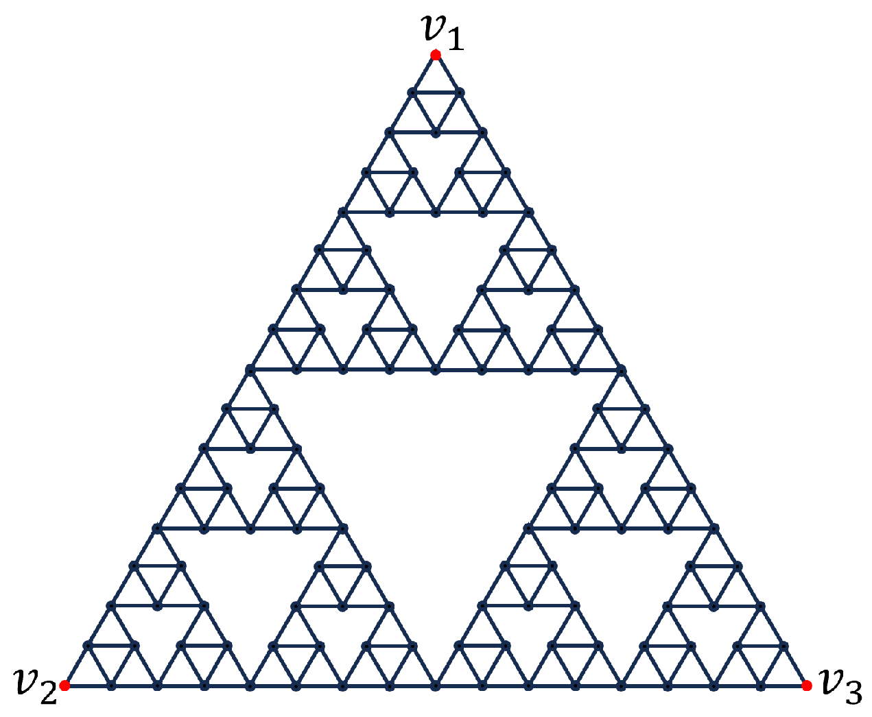
Let $S=\{v_1,v_2,v_3\}$ be the set of initial nodes of skeleton networks $S{G}_{\infty }$ of a Sierpiński gasket, as shown in Figure 3. Using Corollary 2, it is evident that ${\dim }_H(S;\tilde{G})=\log 3/\log 2$.

Example 7.

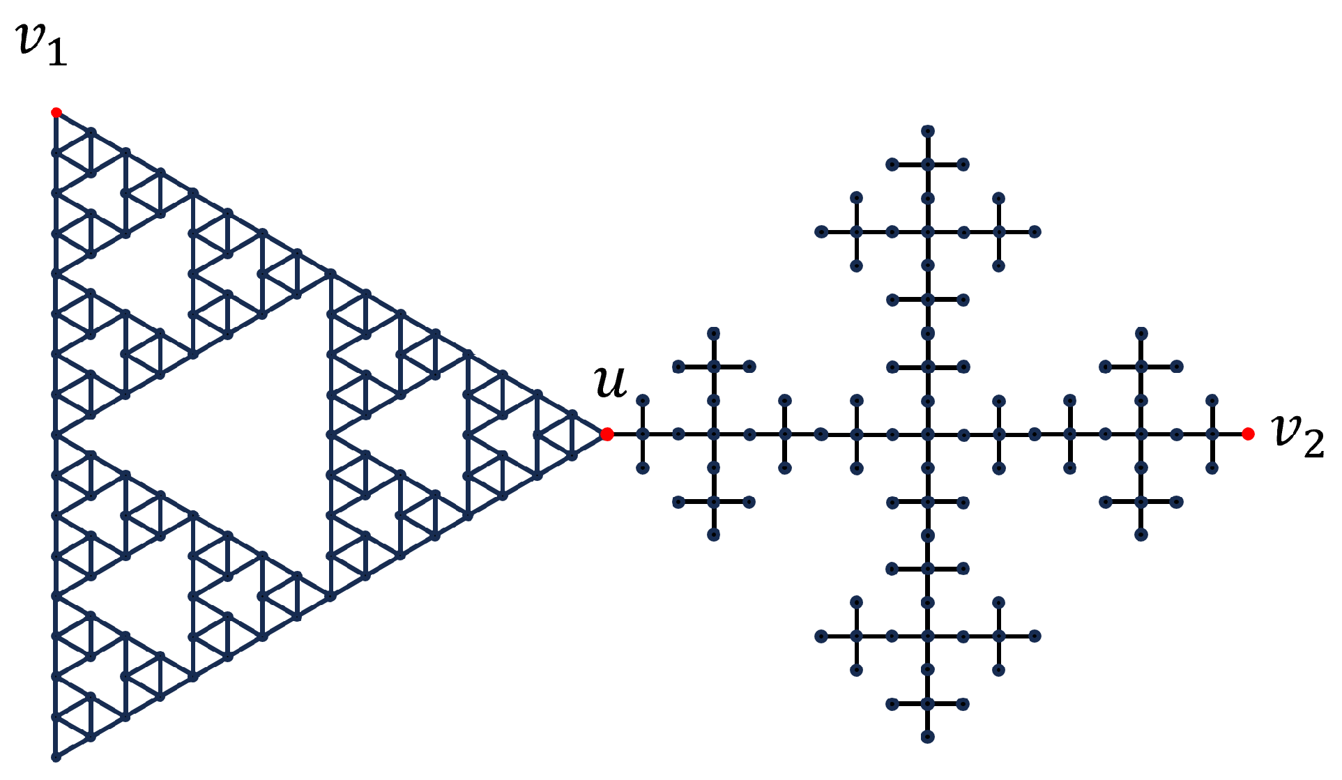
We construct a new fractal network $\tilde{G}$ by connecting a diametral node of $S{G}_{\infty }$ and a diametral node of the Vicsek fractal, $VF$, together, as illustrated in Figure 4. It is easy to check that ${\dim }_H(v_1;\tilde{G})=\log 3/\log 2$ and ${\dim }_H(v_2;\tilde{G})=\log 5/\log 3$. Note that $\log 3/\log 2>\log 5/\log 3$. Then, by Theorem 5, ${\dim }_H(u;\tilde{G})=\log 3/\log 2$, and by Corollary 3, ${\dim }_H(\{v_1,v_2\};\tilde{G})=\log 3/\log 2$.

5. Conclusions

In this paper, we give the $\alpha$-potential of a node on a graph and the $\alpha$-energy of the graph through potential theory. Based on the two definitions, ${\dim }_H(v,\tilde{G})$ and ${\dim }_H\left(\left\{G_n\right\}\right)$ have been proposed. To a certain extent, we also refer to ${\dim }_H(v,\tilde{G})$ as the potential dimension of node v and ${\dim }_H\left(\left\{G_n\right\}\right)$ as the energy dimension of network family $\left\{G_n\right\}$. We list some basic properties of the local Hausdorff dimension. Moreover, some Ahlfors regular networks have been discussed. One can easily check that for a $\alpha$-Ahlfors regular network $\tilde{G}$,

$${\dim }_H(v;\tilde{G})=d_v=\alpha ,$$

and for a family of $\alpha$-Ahlfors regular networks,

$${\dim }_H\left(\left\{G_n\right\}\right)={\dim }_B\left(\left\{G_n\right\}\right)=\alpha ,$$

where ${\dim }_B\left(\left\{G_n\right\}\right)$ represents the box dimension of $\left\{G_n\right\}$. For general networks, we always have ${\dim }_H(v;\tilde{G})\le {\overline{d}}_v$, where ${\overline{d}}_v$ is the upper local dimension of $v\in \tilde{G}$.

A more generalized definition of the local Hausdorff dimension of a subset (or the subset Hausdorff dimension) has been introduced. Propositions 4 and 5 suggest a significant dependence of the subset Hausdorff dimension on the local Hausdorff dimension.

From Corollaries 2 and 3, we can propose two new dimensions pertaining to infinite fractal networks:

$$\begin{array}{c}\hfill {\overline{\dim }}_H\left(\tilde{G}\right)=\underset{v\in \tilde{G}}{sup}{\dim }_H(v;\tilde{G}),\\ \hfill {\underline{\dim }}_H\left(\tilde{G}\right)=\underset{v\in \tilde{G}}{inf}{\dim }_H(v;\tilde{G}).\end{array}$$

If the network $\tilde{G}$ is sufficiently homogeneous, then ${\overline{\dim }}_H\left(\tilde{G}\right)$ should equal ${\underline{\dim }}_H\left(\tilde{G}\right)$.

These dimensions, defined based on distance and $\epsilon$-covering, exhibit many differences in their behavior with respect to fractals and networks. The primary reason for this is that both $d(u,v)$ and $\epsilon$ can be sufficiently small in fractals, whereas in networks, they generally have a lower bound greater than 0. (For example, in an unweighted graph, $d(u,v)$ and $\epsilon$ are at least 1.)

In practical theoretical research, local Hausdorff dimension ${\dim }_H(v;\tilde{G})$ can be applied to analyze the asymptotic behavior of random walks, heat kernel estimates and diffusion processes on infinite networks. It also provides a rigorous dimensional criterion for the finiteness of $\alpha$-potential and $\alpha$-energy on graphs, which complements the discrete version of Frostman lemmas in graph settings.

The metric used in these dimensions can be modified by defining the network distance as a product metric, i.e., a Bowen metric, among others. The function $f\left(x\right)=x^{\alpha }$ involved in $\alpha$-energy and $\alpha$-potential can be replaced by the generalized fractal dimension functions, as seen in [7,8,23]. The study of such dimensions, defined based on potential theory, is of great significance. They are also inherently related to traditional dimensions. Further research is therefore urgently required.

References

1. Mandelbrot, B. How long is the coast of Britain? Statistical self-similarity and fractional dimension. Science 1967, 156, 636–638. [Google Scholar] [CrossRef]
2. Hausdorff, F. Dimension und äußeres Maß. Math. Ann. 1918, 79, 157–179. [Google Scholar] [CrossRef]
3. Pontrjagin, L.; Schnirelmann, L. Sur une propriété métrique de la dimension. Ann. Math. 1932, 33, 156–162. [Google Scholar] [CrossRef]
4. Tricot, C. Two definitions of fractional dimension. Math. Proc. Camb. Philos. Soc. 1982, 91, 57–74. [Google Scholar] [CrossRef]
5. Assouad, P. Espaces Métriques, Plongements, Facteurs. Ph.D. Thesis, Universié Paris XI, Orsay, France, 1977. (In French) [Google Scholar]
6. Lü, F.; Xi, L.F. Quasi-Assouad dimension of fractals. J. Fractal Geom. 2016, 3, 187–215. [Google Scholar] [CrossRef]
7. Achour, R.; Li, Z.M.; Selmi, B. Variational Principles for General Fractal Dimensions. Results Math. 2024, 79, 261. [Google Scholar] [CrossRef]
8. Selmi, B. General multifractal dimensions of measures. Fuzzy Sets Syst. 2025, 499, 109177. [Google Scholar] [CrossRef]
9. Frostman, O. Potential d’équilibre et capacité des ensembles avec quelques applications à la théorie des fonctions. Meddel. Lunds Univ. Math. Sem. 1935, 3, 1–118. [Google Scholar]
10. Song, C.M.; Havlin, S.; Makse, H.A. Self-similarity of complex networks. Nature 2005, 433, 392–395. [Google Scholar] [CrossRef]
11. Wei, D.J.; Wei, B.; Hu, Y.; Zhang, H.X.; Deng, Y. A new information dimension of complex networks. Phys. Lett. A 2014, 378, 1091–1094. [Google Scholar] [CrossRef]
12. Lacasa, L.; Gómez-Gardenes, J. Correlation dimension of complex networks. Phys. Rev. Lett. 2013, 110, 168703. [Google Scholar] [CrossRef]
13. Wei, D.J.; Wei, B.; Zhang, H.X.; Gao, C.; Deng, Y. A generalized volume dimension of complex networks. J. Stat. Mech. Theory Exp. 2014, 2014, P10039. [Google Scholar] [CrossRef]
14. Wu, Y.P.; Chen, Z.L.; Yao, K.; Zhao, X.D.; Chen, Y.C. On the correlation between fractal dimension and robustness of complex networks. Fractals 2019, 27, 1950067. [Google Scholar] [CrossRef]
15. de la Torre, S.R.; Kalda, J.; Kitt, R.; Engelbrecht, J.Y. Fractal and multifractal analysis of complex networks: Estonian network of payments. Eur. Phys. J. B 2017, 90, 234. [Google Scholar]
16. Barlow, M.T.; James, T.S. Defining Fractal Subsets of Zd. Proc. Lond. Math. Soc. 1992, 1, 125–152. [Google Scholar]
17. Jiang, K.; Miao, J.J.; Xi, L.F. Discrete fractals: Dimensions, quasi-isometric invariance and self-similarity. Adv. Math. 2026, 488, 110791. [Google Scholar] [CrossRef]
18. Caldarola, F. The exact measures of the Sierpiński d-dimensional tetrahedron in connection with a Diophantine nonlinear system. Commun. Nonlinear Sci. Numer. Simul. 2018, 63, 228–238. [Google Scholar] [CrossRef]
19. Zeng, Q.C.; Xi, L.F. Hausdorff dimension of a family of networks. Fractals 2023, 31, 2350016. [Google Scholar] [CrossRef]
20. Falconer, F. Fractal Geometry: Mathematical Foundations and Applications, 3rd ed.; John Wiley and Sons: Hoboken, NJ, USA, 2014. [Google Scholar]
21. Jürgensen, H.; Staiger, L. Local Hausdorff dimension. Acta Inf. 1995, 32, 491–507. [Google Scholar]
22. Olsen, L. Characterization of local dimension functions of subsets of Rd. Coll. Math. J. 2005, 103, 231–239. [Google Scholar]
23. Achour, R.; Selmi, B. Exploring simultaneous characterizations of the generalized local fractal dimension functions. Discret. Contin. Dyn. Syst.-Ser. S 2026, 25, 79–93. [Google Scholar]
24. Silva, F.N.; Costa, L.d.F. Local dimension of complex networks. arXiv 2012, arXiv:1209.2476. [Google Scholar]
25. Wen, T.; Jiang, W. Identifying influential nodes based on fuzzy local dimension in complex networks. Chaos Solitons Fractals 2019, 119, 332–342. [Google Scholar]
26. Wen, T.; Deng, Y. Identification of influencers in complex networks by local information dimensionality. Inf. Sci. 2020, 512, 549–562. [Google Scholar] [CrossRef]
27. Wen, T.; Pelusi, D.; Deng, Y. Vital spreaders identification in complex networks with multi-local dimension. Knowl.-Based Syst. 2020, 195, 105717. [Google Scholar] [CrossRef]
28. Xu, K.X.; Das, K.C.; Trinajstić, N. The Harary Index of a Graph; Springer: Heidelberg, Germany, 2015. [Google Scholar]
29. Cui, Z.; Liu, B. On Harary matrix, Harary index and Harary energy. MATCH Commun. Math. Comput. Chem. 2012, 68, 815–823. [Google Scholar]
30. Blumen, A.; Von Ferber, C.; Jurjiu, A.; Koslowski, T. Generalized Vicsek fractals: Regular hyperbranched polymers. Macromolecules 2004, 37, 638–650. [Google Scholar]
31. Trinajstic, N. Chemical Graph Theory; CRC Press: Boca Raton, FL, USA, 2018. [Google Scholar]
Figure 1. The first three levels of the Sierpiński gasket and their related skeleton networks.
Axioms 15 00402 g001
Figure 2. The first three levels of the Vicsek fractal.
Axioms 15 00402 g002
Figure 3. The initial nodes v 1 , v 2 , v 3 of S G .
Axioms 15 00402 g003
Figure 4. G ˜ = S G + u V F .
Axioms 15 00402 g004
Disclaimer/Publisher’s Note: The statements, opinions and data contained in all publications are solely those of the individual author(s) and contributor(s) and not of MDPI and/or the editor(s). MDPI and/or the editor(s) disclaim responsibility for any injury to people or property resulting from any ideas, methods, instructions or products referred to in the content.