q-Close-to-Convexity and Starlikeness of Rabotnov Function

Abstract

The article derives sufficient conditions under which the normalized Rabotnov function becomes q-close-to-convex relative to specific starlike functions on the open unit disk. To enhance the impact of our results, we include some consequences derived from the main theorems, along with graphical illustrations. The starlikeness of the Rabotnov function with respect to different aspects also falls within the scope of this study.

1. Introduction and Preliminaries

Set $H\left(\mathcal{U}\right)$ stands for the family of analytic functions in $\mathcal{U}=\{\mathfrak{z}\in \mathbb{C}:|\mathfrak{z}|<1\}$. A function $\mathfrak{h}\in H\left(\mathcal{U}\right)$ belongs to the class if it obeys the normalizations $\mathfrak{h}\left(0\right)=0$ and ${\mathfrak{h}}^{\prime }\left(0\right)=1$. Any $\mathfrak{h}\in \mathcal{A}$ can be represented as:

$$\mathfrak{h}\left(\mathfrak{z}\right)=\mathfrak{z}+a_2{\mathfrak{z}}^2+a_3{\mathfrak{z}}^3+a_4{\mathfrak{z}}^4+\cdots ,\left|\mathfrak{z}\right|<1.$$

(1)

The subclass $\mathcal{S}$ of $\mathcal{A}$ contains exactly those functions univalent in $\mathcal{U}$. A function $\mathfrak{h}\in \mathcal{A}$ is termed starlike relative to $w_0$ provided that $\mathfrak{h}\left(\mathcal{U}\right)$ is a domain exhibiting starlikeness around $w_0$. In a parallel manner, a function $\mathfrak{h}\in \mathcal{A}$ is referred to as convex when $\mathfrak{h}\left(\mathcal{U}\right)$ happens to be a convex domain. The notation S* is used for the collection of all starlike functions, while C stands for the collection of all convex functions. For $0\le \alpha <1$, the classes S*(α) and $C\left(\alpha \right)$ denote the subsets of S whose members are, respectively, starlike and convex functions of order $\alpha$.

The notion of normalized q-starlike functions originally appeared in the work of Ismail et al. [1] on q-calculus, where they employed the q-difference operator $D_q$. Given an $\mathfrak{h}$, the operator $D_q$ takes the form

$$\left(D_q\mathfrak{h}\right)\left(\mathfrak{z}\right)=\left\{\begin{array}{cc}{\displaystyle \frac{\mathfrak{h}\left(\mathfrak{z}\right)-\mathfrak{h}\left(q\mathfrak{z}\right)}{\mathfrak{z}(1-q)}},\hfill & \mathfrak{z}\in \mathcal{U}\setminus \left\{0\right\},0<q<1,\hfill \\ {\mathfrak{h}}^{\prime }\left(0\right),\hfill & \mathfrak{z}=0,0<q<1,\hfill \end{array}\right.$$

(2)

Observing the configuration of Equation (2), one readily notices that

$$\underset{q\to 1^{-}}{lim}\left\{\left(D_q\mathfrak{h}\right)\left(\mathfrak{z}\right)\right\}={\mathfrak{h}}^{\prime }\left(\mathfrak{z}\right),\mathfrak{z}\in \mathcal{U}.$$

The q-difference operator $D_q$ allows us to define the class ${\mathcal{S}}_q^{\ast }$ of q-starlike functions and the class ${\mathcal{K}}_q$ of q-close-to-convex functions as follows:

We say that $\mathfrak{h}\in \mathcal{A}$ lies in the q-starlike family ${\mathcal{S}}_q^{\ast }$ whenever the following condition holds:

$$\mathrm{For}\mathfrak{z}\in \mathcal{U},0<q<1,\left|{\displaystyle \frac{\mathfrak{z}}{\mathfrak{h}\left(\mathfrak{z}\right)}}\left(D_q\mathfrak{h}\right)\left(\mathfrak{z}\right)-{\displaystyle \frac{1}{1-q}}\right|\le {\displaystyle \frac{1}{1-q}}.$$

(3)

A function $\mathfrak{h}$ belongs to ${\mathcal{K}}_q$, the q-close-to-convex class, whenever it is possible to find a function $g\in {\mathcal{S}}^{\ast }$ such that the condition below holds:

$$\left|{\displaystyle \frac{\mathfrak{z}}{g\left(\mathfrak{z}\right)}}\left(D_q\mathfrak{h}\right)\left(\mathfrak{z}\right)-{\displaystyle \frac{1}{1-q}}\right|\le {\displaystyle \frac{1}{1-q}}\left(\mathfrak{z}\in \mathcal{U},0<q<1\right).$$

(4)

It should be noted that, in the limit $q\to 1^{-}$, the class ${\mathcal{K}}_q$ defined in (4) reduces to the classical close-to-convex class $\mathcal{K}$ associated with the starlike function h. For $0\le \alpha <1$, the familiar classes ${\mathcal{S}}^{\ast }\left(\alpha \right)$, $\mathcal{C}\left(\alpha \right)$, and $\mathcal{K}\left(\alpha \right)$ comprise functions $\mathfrak{h}\in \mathcal{A}$ that satisfy the following, respectively:

$$\Re \left({\displaystyle \frac{\mathfrak{z}{\mathfrak{h}}^{\prime }\left(\mathfrak{z}\right)}{\mathfrak{h}\left(\mathfrak{z}\right)}}\right)>\alpha ,\Re \left(1+{\displaystyle \frac{\mathfrak{z}{\mathfrak{h}}^{\prime \prime }\left(\mathfrak{z}\right)}{{\mathfrak{h}}^{\prime }\left(\mathfrak{z}\right)}}\right)>\alpha ,\Re \left({\displaystyle \frac{\mathfrak{z}{\mathfrak{h}}^{\prime }\left(\mathfrak{z}\right)}{g\left(\mathfrak{z}\right)}}\right)>\alpha (g\in {\mathcal{S}}^{\ast }),$$

for all $\mathfrak{z}\in \mathcal{U}$. We begin by summarizing certain fundamental aspects of quantum calculus (referred to as q-calculus), presenting the main definitions and ideas that support the development in this work. For a function whose domain lies in a subset of $\mathbb{C}$, Jackson’s q-derivatives are respectively defined by

$$D_q\mathfrak{h}\left(\mathfrak{z}\right)={\displaystyle \frac{\mathfrak{h}\left(\mathfrak{z}\right)-\mathfrak{h}\left(\mathfrak{z}q\right)}{\mathfrak{z}(1-q)}}.$$

(5)

Special functions carry considerable weight in mathematical physics and other related fields. These functions, while lacking a universal formal definition, are widely recognized and named within the mathematical community. The category of special functions typically includes elementary functions, especially trigonometric functions, which are often considered foundational. The development of the theory of special functions saw significant progress in the 19th century through the contributions of mathematicians such as Gauss, Jacobi, and Klein. It is their remarkable properties that have allowed these functions to be utilized for centuries. As an illustration, trigonometric functions have found application for more than a millennium, notably in the domain of astronomical calculations. Beginning in the early 1900s, mathematical research progressively shifted toward areas such as topological structures, algebraic systems, the theory of differential equations, and real and functional analysis, as well as investigations involving special functions. A significant contribution to this area is the monograph by G.N. Watson [2], which continues to serve as a fundamental reference, particularly regarding the asymptotic behavior of Bessel functions. The extensive use of hypergeometric and Bessel functions across probability theory and mathematical physics is largely due to their versatility and strong analytical properties. Because of their wide applicability, the Hungarian mathematician Paul Turán once suggested that the term “special functions” is somewhat misleading, proposing instead the more appropriate label “useful functions.”

The Mittag-Leffler (ML) function, a prominent special function, is widely used to solve fractional-order integral equations, as its deep ties to fractional calculus and its effectiveness in solving complex problems across many applications have made it an object of intense investigation in modern times. Thanks to the ML-function and its diverse generalizations, scientists in recent decades have effectively solved a wide variety of challenges arising in physics, engineering, chemistry, biology, and other applied areas. This widespread applicability has greatly increased its prominence within the scientific community. As a result, these functions have become the subject of extensive research, with many scholars exploring them from a rigorous mathematical standpoint [3]. An extension of the basic Mittag-Leffler function is given by the two-parameter ML-function $E_{\alpha ,\beta }$, for $\alpha ,\beta ,\mathfrak{z}\in \mathbb{C}$ is as follows:

$$E_{\alpha ,\beta }\left(\mathfrak{z}\right)={\displaystyle \sum _{\mathfrak{m}=0}^{\infty }}{\displaystyle \frac{{\mathfrak{z}}^{\mathfrak{m}}}{\mathrm{\Gamma }(\alpha \mathfrak{m}+\beta )}}.$$

A function based on the ML-function was introduced in 1949 by Yuriy Nicholaevich Rabotnov, a Russian researcher celebrated for his extensive work in solid mechanics. The Rabotnov function is defined as a power series involving the gamma function $\left(\mathrm{\Gamma }\right)$ [4]:

$$R_{\alpha ,\beta }\left(\mathfrak{z}\right)={\mathfrak{z}}^{\alpha }{\displaystyle \sum _{\mathfrak{m}=0}^{\infty }}{\displaystyle \frac{{\beta }^{\mathfrak{m}}}{\mathrm{\Gamma }\left((1+\mathfrak{m})(1+\alpha )\right)}}{\mathfrak{z}}^{\mathfrak{m}(\alpha +1)},\alpha ,\beta ,\mathfrak{z}\in \mathbb{C}.$$

This series clearly converges for any argument. It becomes the usual exponential $exp\left(\beta \mathfrak{z}\right)$ when $\alpha =0$. One connection between $R_{\alpha ,\beta }$ and $E_{\alpha ,\beta }$ can be expressed as follows:

$$R_{\alpha ,\beta }\left(\mathfrak{z}\right)={\mathfrak{z}}^{\alpha }{E}_{1+\alpha ,1+\beta }\left(\beta {\mathfrak{z}}^{1+\alpha }\right),\alpha ,\beta ,\mathfrak{z}\in \mathbb{C}.$$

In the realm of function theory, functions including hypergeometric, Bessel, and Mittag-Leffler types occupy an essential place. A prominent illustration of their significance is their role in the proof of the classical Bieberbach conjecture, achieved through the work of L. de Branges’s surprising deployment of hypergeometric functions which sparked considerable interest in generalized, Kummer, and Gauss hypergeometric functions, specifically regarding their geometric properties, as well as various other related functions. While the geometric features of these functions are fascinating on their own, they have demonstrated their usefulness in solving a wide variety of additional issues arising in function theory. In recent years, the geometric properties and applications of the ML-function and its related forms have attracted significant scholarly interest. Given that the Rabotnov function can be expressed as a combination of ML-functions, it is natural to explore recent advances concerning the geometric characteristics of ML-functions. Liu et al. [5] and Bansal [6] examined certain geometric aspects of that type of function, while Raducanu [7] focused on their partial sums. Noreen et al. [8] conducted extensive investigations into their geometric behavior, with further refinements and improvements later contributed by Das and Mehrez [9]. Additionally, Srivastava et al. [10] explored a generalized version involving a three-parameter ML-function. Recently, the geometric properties of the Rabotnov functions were explored in [11,12]. Frasin [13] investigated the partial sums of a generalized form of the Rabotnov function. Particular subclasses of bi-univalent functions that involve this function were investigated by Amourah et al. [14]. In a separate study, Deniz and Kazımoğlu [15] analyzed Hardy spaces by means of a distinct methodology founded upon the Rabotnov function. Very recently, Raza et. al. [16] discussed the geometric properties and hardy spaces of the Rabotnov function. Geometric properties have become a highly active and popular area of research in recent times. For the sake of our analysis, we consider the Rabotnov function normalized as follows:

$$\begin{array}{ccc}\hfill {\mathcal{R}}_{\alpha ,\beta }\left(\mathfrak{z}\right)& =& {\mathfrak{z}}^{{\displaystyle \frac{1}{1+\alpha }}}\mathrm{\Gamma }(1+\alpha )R_{\alpha ,\beta }\left({\mathfrak{z}}^{{\displaystyle \frac{1}{1+\alpha }}}\right),\hfill \\ & =& \mathfrak{z}+{\displaystyle \sum _{\mathfrak{m}=2}^{\infty }}{\displaystyle \frac{{\beta }^{\mathfrak{m}-1}\mathrm{\Gamma }(\alpha +1)}{\mathrm{\Gamma }\left((1+\alpha )\mathfrak{m}\right)}}{\mathfrak{z}}^{\mathfrak{m}}.\hfill \end{array}$$

Here, we define some particular cases of the normalized Rabotnov function.

$$\begin{array}{ccc}\hfill {\mathcal{R}}_{0,1}(\mathfrak{z})& =& \mathfrak{z}{e}^{\mathfrak{z}},\hfill \\ \hfill {\mathcal{R}}_{1,1}(\mathfrak{z})& =& \sqrt{\mathfrak{z}}sinh(\sqrt{\mathfrak{z}}),\hfill \\ \hfill {\mathcal{R}}_{1,2}(\mathfrak{z})& =& \sqrt{{\displaystyle \frac{\mathfrak{z}}{2}}}sinh(\sqrt{2\mathfrak{z}}),\hfill \\ \hfill {\mathcal{R}}_{1,{\displaystyle \frac{1}{2}}}(\mathfrak{z})& =& {\displaystyle \frac{4sinh(\frac{\sqrt{\mathfrak{z}}}{2})}{\sqrt{\mathfrak{z}}}}.\hfill \end{array}$$

The q-close-to-convexity connected to the q-hypergeometric function began in [17]. Later, Srivastava et al. [18], and Raza et al. [19], extended it to q-ML-functions. Later, Din et al. [20] extended the analysis to q-Bessel–Wright functions, whereas Noreen et al. [21] performed an analogous study for the q-Bessel–Struve function. Inspired by these findings, in this work, we investigated the q-close-to-convexity of the Rabotnov function with respect to particular starlike functions.

Close-to-convex functions generalize convex ones. While every convex function is univalent, close-to-convexity relative to a starlike function—without requiring convexity or starlikeness—still ensures univalence and other geometric traits. This provides a practical criterion for proving univalence. Many special functions (e.g., Bessel, Struve, hypergeometric) may not be starlike or convex, yet can be close-to-convex to some starlike function, offering a sufficient condition for univalence. This approach also helps derive inclusion relations among analytic function classes.

From an analytic viewpoint, a function $\mathfrak{h}$ is called close-to-convex with respect to a starlike function k if it satisfies $Re\left({\displaystyle \frac{\mathfrak{z}{\mathfrak{h}}^{\prime }\left(\mathfrak{z}\right)}{k\left(\mathfrak{z}\right)}}\right)>0$. It is classical that ${\mathfrak{g}}_1\left(\mathfrak{z}\right)={\displaystyle \frac{\mathfrak{z}}{1-\mathfrak{z}}}$ is both starlike and convex, whereas ${\mathfrak{g}}_2\left(z\right)={\displaystyle \frac{z}{1-z^2}}$ is starlike but not convex. Consequently, taking $k\left(\mathfrak{z}\right)$ as either ${\mathfrak{k}}_1\left(\mathfrak{z}\right)$ or ${\mathfrak{k}}_2\left(\mathfrak{z}\right)$ makes $\mathfrak{z}/\mathfrak{k}\left(\mathfrak{z}\right)$ reduce to $(1-\mathfrak{z})$ and $(1-{\mathfrak{z}}^2)$, respectively, thereby significantly simplifying coefficient-related calculations for $\mathfrak{h}$.

Next, assume that $\mathfrak{h}$ is univalent in $\mathcal{U}$.We call $\mathfrak{h}$ convex in the direction of the imaginary axis provided that every vertical line (that is, any line parallel to the imaginary axis) intersects the image region $\mathfrak{h}\left(\mathcal{U}\right)$ in a set that is either empty or connected. The following key lemmas serve as the foundation for the principal findings presented herein.

Lemma 1 

([18]). Suppose a sequence $\left(A_{\mathfrak{m}}\right)$ of real numbers is given. Define

$$B_{\mathfrak{m}}={\displaystyle \frac{A_{\mathfrak{m}}(1-q^{\mathfrak{m}})}{1-q}},\forall \mathfrak{m}\in \mathbb{N},q\in (0,1).$$

Assume that either

$$1\ge B_1\ge B_2\ge B_3\ge \cdots \ge B_{\mathfrak{m}}\ge \cdots \ge 0$$

or

$$1\le B_1\le B_2\le B_3\le \cdots \le B_{\mathfrak{m}}\le \cdots \le 2.$$

Then

$$\mathfrak{h}\left(\mathfrak{z}\right)={\displaystyle \sum _{\mathfrak{m}=2}^{\infty }}{A}_{\mathfrak{m}}{\mathfrak{z}}^{\mathfrak{m}}$$

belongs to ${\mathcal{K}}_{q,p}$ with respect to

$$p\left(\mathfrak{z}\right)={\displaystyle \frac{\mathfrak{z}}{1-\mathfrak{z}}}.$$

Lemma 2 

([17]). Given a real sequence $\left(A_{\mathfrak{m}}\right)$, set

$$B_{\mathfrak{m}}={\displaystyle \frac{A_{\mathfrak{m}}(1-q^{\mathfrak{m}})}{1-q}},\mathfrak{m}\in \mathbb{N},q\in (0,1).$$

Assume that for all odd indices $2\mathfrak{m}-1$ ($\mathfrak{m}\ge 2$), the subsequence $\left\{B_{2\mathfrak{m}-1}\right\}$ satisfies one of the following two monotonicity conditions:

(Condition A)

$$0\le \cdots \le B_{2\mathfrak{m}-1}\le \cdots \le B_5\le B_5\le B_3\le 1.$$

(Condition B)

$$2\ge \cdots \ge B_{2\mathfrak{m}-1}\ge \cdots \ge B_5\ge B_5\ge B_3\ge 1.$$

Then

$$\mathfrak{h}\left(\mathfrak{z}\right)={\displaystyle \sum _{\mathfrak{m}=2}^{\infty }}{A}_{2\mathfrak{m}-1}{\mathfrak{z}}^{2\mathfrak{m}-1}\in {\mathcal{K}}_{q,\mathfrak{h}}$$

with respect to

$$\mathfrak{h}\left(\mathfrak{z}\right)={\displaystyle \frac{\mathfrak{z}}{1-{\mathfrak{z}}^2}}.$$

Lemma 3 

([22]). Assume $a_{\mathfrak{m}}\ge 0$ and that the sequences $\left\{\mathfrak{m}{a}_{\mathfrak{m}}\right\}$ and $\{\mathfrak{m}{a}_{\mathfrak{m}}-(\mathfrak{m}+1)a_{\mathfrak{m}+1}\}$ are non-increasing. Then $\mathfrak{h}\left(\mathfrak{z}\right)=\mathfrak{z}+a_2{\mathfrak{z}}^2+a_3{\mathfrak{z}}^3+\cdots$ ($\mathfrak{z}\in \mathcal{U}$) falls within the class ${\mathcal{S}}^{\ast }$.

Lemma 4 

([23]). Assume $\beta \ge 0$ and $\mu \in \mathbb{R}$ with $0<\mu +\beta <1$, and fix $n\in \mathbb{N}$. Set $d_0=d_1=1$. For $1\le k\le n$, put

$$d_{2k}=d_{2k+1}={\displaystyle \frac{n!{(1+\beta )}_{n-k}}{(n-k)!{(1+\beta )}_n}}·{\displaystyle \frac{{(\mu +\beta )}_k}{k!}}.$$

Then the statements below are true:

(i) 

${\displaystyle {\displaystyle \sum _{k=0}^n}{d}_{k}cos\left(k\theta \right)>0}$ holds exactly when $\mu +\beta \le {\mu }^{\ast }\left(\frac{1}{2}\right)=0.691556\dots$

(ii) 

${\displaystyle {\displaystyle \sum _{k=1}^{2n+1}}sin\left(k\theta \right)>0}$ holds exactly when $\mu +\beta \le {\mu }^{\ast }\left(\frac{1}{2}\right)$

(iii) 

${\displaystyle {\displaystyle \sum _{k=1}^{2n}}sin\left(k\theta \right)>0}$ holds provided $\mu +\beta \le {\displaystyle \frac{1+\beta }{2}}$.

In the above, for any $\gamma \in (0,1]$, the quantity ${\mu }^{\ast }\left(\gamma \right)$ stands for the unique root in $(0,1)$ of the equation

$${{\displaystyle \mathit{\int }}}_0^{(\gamma +1)\pi }{\displaystyle \frac{sin\left(t-\gamma \pi \right)}{t^{1-\mu }}}dt=0.$$

One notes that ${\mu }^{\ast }\left(\gamma \right)$ originally appeared in the work of Koumandos and Ruscheweyh [24]. The present study makes extensive use of the special case ${\mu }^{\ast }\left({\displaystyle \frac{1}{2}}\right)={\mu }_0^{\ast }$.

Lemma 5 

([23]). Assume $0\le \beta \le 2{\mu }_0^{\ast }-1$ and $-\beta <\mu \le {\displaystyle \frac{1-\beta }{2}}$, with $a_1=1$ and $a_k\ge 0$ for all k. For $1\le k\le n$, the following conditions hold:

$$\begin{array}{cc}\hfill {\displaystyle \frac{a_k}{a_{k+1}}}& \ge {\displaystyle \frac{(k+1)(1+\beta )(1-\mu -\beta )-1+2\mu +\beta }{k(1+\beta )(1-\mu -\beta )-1+2\mu +\beta }},if{a}_{k+1}>0,\hfill \end{array}$$

(6)

$$\begin{array}{cc}\hfill {\displaystyle \frac{a_{2k}}{a_{2k+1}}}& \ge {\displaystyle \frac{k(n-k+1+\beta )\left[(2k+1)(1+\beta )(1-\mu -\beta )-1+2\mu +\beta \right]}{(n-k+1)(k+\mu +\beta -1)\left[2k(1+\beta )(1-\mu -\beta )-1+2\mu +\beta \right]}},if{a}_{2k+1}>0.\hfill \end{array}$$

(7)

(If any denominator $a_{k+1}$ or $a_{2k+1}$ equals zero, the corresponding inequality is automatically satisfied.)

Then the polynomial ${\mathfrak{h}}_n\left(\mathfrak{z}\right)={\sum }_{k=1}^n{a}_k{\mathfrak{z}}^k$ is starlike of order ${\displaystyle \frac{1-2\mu -\beta }{(1+\beta )(1-\mu -\beta )}}$.

In the limiting case $n\to \infty$, the function $\mathfrak{h}\left(\mathfrak{z}\right)={\sum }_{k=1}^{\infty }{a}_k{\mathfrak{z}}^k$ remains starlike of the same order, provided (6) holds for all $k\ge 1$ together with the additional requirement for $k\ge 1$:

$$\begin{array}{cc}\hfill {\displaystyle \frac{a_{2k}}{a_{2k+1}}}& \ge {\displaystyle \frac{k\left[(2k+1)(1+\beta )(1-\mu -\beta )-1+2\mu +\beta \right]}{(k+\mu +\beta -1)\left[2k(1+\beta )(1-\mu -\beta )-1+2\mu +\beta \right]}},if{a}_{2k+1}>0.\hfill \end{array}$$

(8)

Lemma 6 

([23]). Let $0\le \beta \le 2{\mu }_0^{\ast }-1$ and $\mu \in \mathbb{R}$ satisfy $0<\mu +\beta <1$, and fix $n\in \mathbb{N}$. Suppose $\left\{a_k\right\}$ is a non negative decreasing sequence with $a_0>0$ satisfying, for $1\le k\le n$,

$${\displaystyle \frac{a_{2k}}{a_{2k-1}}}\le {\displaystyle \frac{(n-k+1)(k+\mu +\beta -1)}{k(n-k+1+\beta )}},if{a}_{2k-1}>0.$$

Then, for every $0<\theta <\pi$,

$${\displaystyle \sum _{k=0}^n}{a}_{k}sin\left(k\theta \right)>0⟺\mu +\beta \le {\displaystyle \frac{1+\beta }{2}}.$$

2. Results

Theorem 1. 

Let $\alpha \ge 1$, $\beta \ge 1$, ${\displaystyle \frac{\mathrm{\Gamma }\left(2\left(\alpha +1\right)\right)}{(1+q)\mathrm{\Gamma }\left(\alpha +1\right)}}\ge \beta$ and with the inequality

$$\left({\displaystyle \frac{1-q^{\mathfrak{m}+1}}{1-q^{\mathfrak{m}}}}\right)\beta \le {\displaystyle \prod _{k=0}^{\alpha }}\left(\left(\alpha +1\right)\mathfrak{m}+k\right),(\mathfrak{m}\in \mathbb{N}-\left\{1\right\}).$$

(9)

Consequently, the normalized Rabotnov function ${\mathcal{R}}_{\alpha ,\beta }\left(\mathfrak{z}\right)$ turns out to be q-close-to-convex on the open unit disk with respect to

$$p\left(\mathfrak{z}\right)={\displaystyle \frac{\mathfrak{z}}{1-\mathfrak{z}}}.$$

Proof. 

Take, for instance, the function

$${\mathcal{R}}_{\alpha ,\beta }\left(\mathfrak{z}\right)=\mathfrak{z}+{\displaystyle \sum _{\mathfrak{m}=2}^{\infty }}{\displaystyle \frac{{\beta }^{m-1}\mathrm{\Gamma }\left(\alpha +1\right)}{\mathrm{\Gamma }\left(\left(\alpha +1\right)\mathfrak{m}\right)}}{\mathfrak{z}}^{\mathfrak{m}}.$$

This expression admits the alternative form

$${\mathcal{R}}_{\alpha ,\beta }\left(\mathfrak{z}\right)=\mathfrak{z}+{\displaystyle \sum _{\mathfrak{m}=2}^{\infty }}{A}_{\mathfrak{m}}{\mathfrak{z}}^{\mathfrak{m}},$$

where

$$A_{\mathfrak{m}}={\displaystyle \frac{{\beta }^{\mathfrak{m}-1}\mathrm{\Gamma }\left(\alpha +1\right)}{\mathrm{\Gamma }\left(\left(\alpha +1\right)\mathfrak{m}\right)}}.$$

To prove that the normalized Rabotnov function is q-close-to-convex, we consider

$$B_{\mathfrak{m}}={\displaystyle \frac{(1-q^{\mathfrak{m}})}{1-q}}{A}_{\mathfrak{m}},\forall \mathfrak{m}\in \mathbb{N},q\in (0,1),$$

thereby

$$B_{\mathfrak{m}}={\displaystyle \frac{(1-q^{\mathfrak{m}})}{1-q}}{\displaystyle \frac{{\beta }^{\mathfrak{m}-1}\mathrm{\Gamma }\left(\alpha +1\right)}{\mathrm{\Gamma }\left(\left(\alpha +1\right)\mathfrak{m}\right)}}.$$

(10)

Note that $B_1=1$ and $B_{\mathfrak{m}}>0$ for all $\mathfrak{m}\in \mathbb{N}$. Furthermore, Lemma 2 yields

$$B_2={\displaystyle \frac{\beta (1+q)\mathrm{\Gamma }\left(\alpha +1\right)}{\mathrm{\Gamma }\left(2\left(\alpha +1\right)\right)}}\le 1.$$

Our next goal is to prove that

$$B_{\mathfrak{m}+1}\le B_{\mathfrak{m}},(\mathfrak{m}\in \mathbb{N}-\left\{1\right\}).$$

From this, it follows that

$${\displaystyle \frac{(1-q^{\mathfrak{m}+1}){\beta }^{\mathfrak{m}}\mathrm{\Gamma }\left(\alpha +1\right)}{(1-q)\mathrm{\Gamma }\left(\left(\alpha +1\right)\left(m+1\right)\right)}}\le {\displaystyle \frac{(1-q^{\mathfrak{m}}){\beta }^{\mathfrak{m}-1}\mathrm{\Gamma }\left(\alpha +1\right)}{(1-q)\mathrm{\Gamma }\left(\left(\alpha +1\right)\mathfrak{m}\right)}},(\mathfrak{m}\in \mathbb{N}-\left\{1\right\}).$$

which is equivalent to

$$\beta (1-q^{\mathfrak{m}+1})\mathrm{\Gamma }\left(\left(\alpha +1\right)\mathfrak{m}\right)\le (1-q^{\mathfrak{m}})\mathrm{\Gamma }\left(\left(\alpha +1\right)\left(\mathfrak{m}+1\right)\right).$$

(11)

To verify the inequality (11), we use the recurrence of Gamma function.

$$\mathrm{\Gamma }\left(\alpha +1\right)=\alpha \mathrm{\Gamma }\left(\alpha \right).$$

Thus,

$$\mathrm{\Gamma }\left(\left(\alpha +1\right)\left(\mathfrak{m}+1\right)\right)={\displaystyle \prod _{k=0}^{\alpha }}\left(\left(\alpha +1\right)\mathfrak{m}+k\right)\mathrm{\Gamma }\left(\left(\alpha +1\right)\mathfrak{m}\right).$$

(12)

By using (11) and (12), it becomes

$$\beta (1-q^{\mathfrak{m}+1})\le (1-q^{\mathfrak{m}}){\displaystyle \prod _{k=0}^{\alpha }}\left(\left(\alpha +1\right)\mathfrak{m}+k\right).$$

(13)

Since, $\alpha \ge 1$ and $\mathfrak{m}\ge 2$

$$\left(\alpha +1\right)\mathfrak{m}+k\ge \left(\alpha +1\right)\mathfrak{m},\forall k\ge 0.$$

Hence,

$${\displaystyle \prod _{k=0}^{\alpha }}\left(\left(\alpha +1\right)\mathfrak{m}+k\right)\ge {\left(\left(\alpha +1\right)\mathfrak{m}\right)}^{\alpha +1}.$$

So, the R.H.S is bounded below:

$$(1-q^{\mathfrak{m}}){\left(\left(\alpha +1\right)\mathfrak{m}\right)}^{\alpha +1}.$$

Given $q\in (0,1)$, we have $q^{\mathfrak{m}+1}<q^{\mathfrak{m}}$, which yields $1-q^{\mathfrak{m}+1}>1-q^{\mathfrak{m}}$. Therefore,

$${\displaystyle \frac{1-q^{\mathfrak{m}+1}}{1-q^{\mathfrak{m}}}}>1.$$

So, the inequality (13) reduces to

$$\beta \le \left({\displaystyle \frac{1-q^{\mathfrak{m}}}{1-q^{\mathfrak{m}+1}}}\right){\left(\left(\alpha +1\right)\mathfrak{m}\right)}^{\alpha +1}.$$

Therefore,

$${\displaystyle \frac{\beta (1-q^{\mathfrak{m}+1})}{1-q^{\mathfrak{m}}}}\le {\displaystyle \prod _{k=0}^{\alpha }}\left((\alpha +1)\mathfrak{m}+k\right),(q\ne 1,\mathfrak{m}\in \mathbb{N}).$$

which completes the proof. □

Corollary 1. 

Let $\alpha =0$, $\beta =1$ and with the inequality

$$\left(1-q^{\mathfrak{m}+1}\right)\le \left(1-q^{\mathfrak{m}}\right)\mathfrak{m},(\mathfrak{m}\in \mathbb{N}-\left\{1\right\}).$$

(14)

Corollary 2. 

Consequently, the normalized Rabotnov function ${\mathcal{R}}_{0,1}\left(\mathfrak{z}\right)=\mathfrak{z}{e}^{\mathfrak{z}}$ satisfies the q-close-to-convexity condition within the open unit disk relative to the function

$$p\left(\mathfrak{z}\right)={\displaystyle \frac{\mathfrak{z}}{1-\mathfrak{z}}}.$$

Corollary 3. 

Let $\alpha =1$, $\beta =1$ and with the inequality

$$\left(1-q^{\mathfrak{m}+1}\right)\le \left(1-q^{\mathfrak{m}}\right)\left(2\mathfrak{m}\right)\left(2\mathfrak{m}+1\right),(\mathfrak{m}\in \mathbb{N}-\left\{1\right\}).$$

(15)

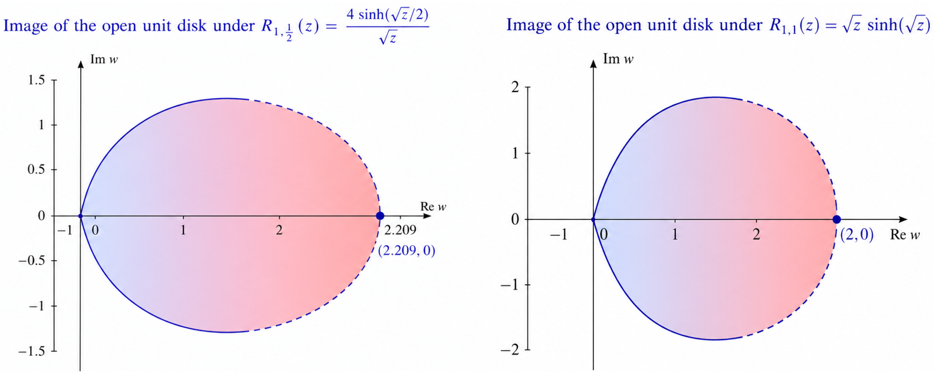
Then ${\mathcal{R}}_{1,1}\left(\mathfrak{z}\right)=\sqrt{\mathfrak{z}}sinh\left(\sqrt{\mathfrak{z}}\right)$ (see Figure 1) is q-close-to-convex on $\mathcal{U}$ with respect to

$$p\left(\mathfrak{z}\right)={\displaystyle \frac{\mathfrak{z}}{1-\mathfrak{z}}}.$$

Corollary 4. 

Let $\alpha =1$, $\beta =2$ and with the inequality

$$\left(1-q^{\mathfrak{m}+1}\right)\le \left(1-q^{\mathfrak{m}}\right)\left(\mathfrak{m}\right)\left(2\mathfrak{m}+1\right),(\mathfrak{m}\in \mathbb{N}-\left\{1\right\}).$$

(16)

Then the function ${\mathcal{R}}_{1,2}\left(\mathfrak{z}\right)=\sqrt{{\displaystyle \frac{\mathfrak{z}}{2}}}sinh\left(\sqrt{2\mathfrak{z}}\right)$ proves to be q-close-to-convex when taken with respect to

$$p\left(\mathfrak{z}\right)={\displaystyle \frac{\mathfrak{z}}{1-\mathfrak{z}}}.$$

Corollary 5. 

Let $\alpha =1$, $\beta ={\displaystyle \frac{1}{2}}$ with

$$\left(1-q^{\mathfrak{m}+1}\right)\le \left(1-q^{\mathfrak{m}}\right)\left(4\mathfrak{m}\right)\left(2\mathfrak{m}+1\right),(\mathfrak{m}\in \mathbb{N}-\left\{1\right\}).$$

(17)

As a specific instance of the Rabotnov function, ${\mathcal{R}}_{1,{\displaystyle \frac{1}{2}}}(\mathfrak{z})={\displaystyle \frac{4sinh(\frac{\sqrt{\mathfrak{z}}}{2})}{\sqrt{\mathfrak{z}}}}$ (see Figure 1) proves to be q-close-to-convex with respect to

$$p\left(\mathfrak{z}\right)={\displaystyle \frac{1}{1-\mathfrak{z}}}-1.$$

Theorem 2. 

Let $\alpha \ge 1$, $\beta \ge 1$, ${\beta }^2\le {\displaystyle \frac{\mathrm{\Gamma }\left(3\left(\alpha +1\right)\right)}{(1+q+q^2)\mathrm{\Gamma }\left(\alpha +1\right)}}$ and with the inequality

$${\beta }^2\left({\displaystyle \frac{1-q^{2\mathfrak{m}+1}}{1-q^{2\mathfrak{m}-1}}}\right)\le {\displaystyle \prod _{k=0}^{2\alpha +1}}\left[\left(\alpha +1\right)\left(2\mathfrak{m}-1\right)+k\right],(\mathfrak{m}\in \mathbb{N}-\left\{1\right\}).$$

(18)

Then ${\mathcal{R}}_{\alpha ,\beta }\left(\mathfrak{z}\right)\in {\mathcal{K}}_{q,\mathfrak{g}}$ in the open unit disk with respect to

$$\mathfrak{g}\left(\mathfrak{z}\right)={\displaystyle \frac{\mathfrak{z}}{1-{\mathfrak{z}}^2}}.$$

Proof. 

Take the function

$${\mathcal{R}}_{\alpha ,\beta }\left(\mathfrak{z}\right)=\mathfrak{z}+{\displaystyle \sum _{\mathfrak{m}=2}^{\infty }}{\displaystyle \frac{{\beta }^{\mathfrak{m}-1}\mathrm{\Gamma }\left(\alpha +1\right)}{\mathrm{\Gamma }\left(\left(\alpha +1\right)\mathfrak{m}\right)}}{\mathfrak{z}}^{\mathfrak{m}}.$$

Another way to write this expression is

$${\mathcal{R}}_{\alpha ,\beta }\left(\mathfrak{z}\right)=\mathfrak{z}+{\displaystyle \sum _{\mathfrak{m}=2}^{\infty }}{A}_{\mathfrak{m}}{\mathfrak{z}}^{\mathfrak{m}},$$

where

$$A_{\mathfrak{m}}={\displaystyle \frac{{\beta }^{\mathfrak{m}-1}\mathrm{\Gamma }\left(\alpha +1\right)}{\mathrm{\Gamma }\left(\left(\alpha +1\right)\mathfrak{m}\right)}}.$$

To prove that ${\mathcal{R}}_{\alpha ,\beta }\left(\mathfrak{z}\right)\in {\mathcal{K}}_{q,\mathfrak{g}}$, we construct

$$B_{\mathfrak{m}}={\displaystyle \frac{A_{\mathfrak{m}}(1-q^{\mathfrak{m}})}{1-q}},\forall \mathfrak{m}\in \mathbb{N},q\in (0,1),$$

so that

$$B_{\mathfrak{m}}={\displaystyle \frac{(1-q^{\mathfrak{m}})}{(1-q)}}{\displaystyle \frac{{\beta }^{\mathfrak{m}-1}\mathrm{\Gamma }\left(\alpha +1\right)}{\mathrm{\Gamma }\left(\left(\alpha +1\right)m\right)}}.$$

(19)

It is easy to verify that $B_1=1$, and that $B_{\mathfrak{m}}>0$ for every positive integer $\mathfrak{m}$. Moreover, Lemma 2 yields the following:

$$B_3={\displaystyle \frac{{\beta }^2(1+q+q^2)\mathrm{\Gamma }\left(\alpha +1\right)}{\mathrm{\Gamma }\left(3\left(\alpha +1\right)\right)}}\le 1.$$

We now turn to proving that

$$B_{2\mathfrak{m}+1}\le B_{2\mathfrak{m}-1},(\mathfrak{m}\in \mathbb{N}-\left\{1\right\}).$$

$$\begin{array}{ccc}& & {\displaystyle \frac{(1-q^{2\mathfrak{m}+1})}{(1-q)}}{\displaystyle \frac{{\beta }^{2\mathfrak{m}}\mathrm{\Gamma }\left(\alpha +1\right)}{\mathrm{\Gamma }\left(\left(\alpha +1\right)\left(2\mathfrak{m}+1\right)\right)}}\hfill \\ & \le & {\displaystyle \frac{(1-q^{2\mathfrak{m}-1})}{(1-q)}}{\displaystyle \frac{{\beta }^{2\mathfrak{m}-2}\mathrm{\Gamma }\left(\alpha +1\right)}{\mathrm{\Gamma }\left(\left(\alpha +1\right)\left(2\mathfrak{m}-1\right)\right)}},(\mathfrak{m}\in \mathbb{N}-\left\{1\right\}),\hfill \end{array}$$

which is the same as

$$(1-q^{2\mathfrak{m}+1})\left({\beta }^2\right)\mathrm{\Gamma }\left(\left(\alpha +1\right)\left(2\mathfrak{m}-1\right)\right)\le (1-q^{2\mathfrak{m}-1})\mathrm{\Gamma }\left(\left(\alpha +1\right)\left(2\mathfrak{m}+1\right)\right).$$

(20)

To verify the (20) inequality, let $x=\alpha +1,$ since, $\alpha \ge 1.$ Then $x\ge 2.$ The following property is used

$$\begin{array}{ccc}\hfill \mathrm{\Gamma }\left(\mathfrak{z}+n\right)& =& \mathrm{\Gamma }\left(\mathfrak{z}\right){\displaystyle \prod _{k=0}^{n-1}}\left(\mathfrak{z}+k\right),\mathrm{where},\mathfrak{z}=x\left(2\mathfrak{m}-1\right)\mathrm{and}n=2x.\hfill \\ \hfill {\displaystyle \frac{\mathrm{\Gamma }\left(\mathfrak{z}+2x\right)}{\mathrm{\Gamma }\left(\mathfrak{z}\right)}}& =& \left(\mathfrak{z}\right)\left(\mathfrak{z}+1\right)\left(\mathfrak{z}+2\right)...\left(\mathfrak{z}+2x-1\right),\hfill \\ & =& {\displaystyle \prod _{k=0}^{2\alpha +1}}\left[\left(\alpha +1\right)\left(2\mathfrak{m}-1\right)+k\right].\hfill \end{array}$$

Since $q\in \left(0,1\right)$ and $q^{2\mathfrak{m}+1}<q^{2\mathfrak{m}-1}$⇒$1-q^{2\mathfrak{m}+1}>1-q^{2\mathfrak{m}-1}.$ Thus,

$${\displaystyle \frac{1-q^{2\mathfrak{m}+1}}{1-q^{2\mathfrak{m}-1}}}>1.$$

Now, Equation (20) becomes

$${\beta }^2\left({\displaystyle \frac{1-q^{2\mathfrak{m}+1}}{1-q^{2\mathfrak{m}-1}}}\right)\le {\displaystyle \prod _{k=0}^{2\alpha +1}}\left[\left(\alpha +1\right)\left(2\mathfrak{m}-1\right)+k\right],$$

which completes the proof. □

Corollary 6. 

Let $\alpha =0$, $\beta =1$, $(1+q+q^2)\le 2$ with the inequality

$$\left({\displaystyle \frac{1-q^{2\mathfrak{m}+1}}{1-q^{2\mathfrak{m}-1}}}\right)\le \left(2\mathfrak{m}\right)\left(2\mathfrak{m}-1\right),(\mathfrak{m}\in \mathbb{N}-\left\{1\right\}).$$

(21)

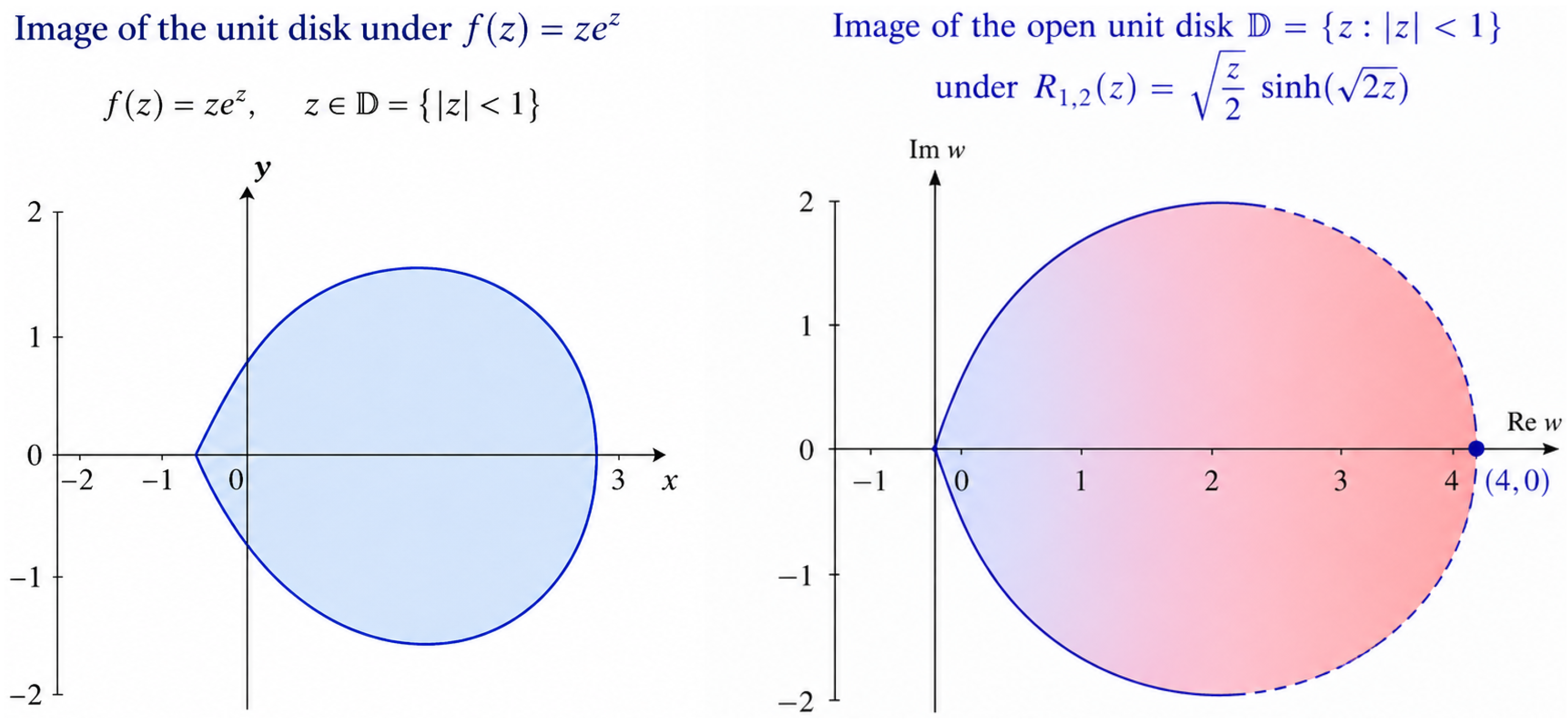
Then the function ${\mathcal{R}}_{\alpha ,\beta }\left(\mathfrak{z}\right)\in {\mathcal{K}}_{q,\mathfrak{g}}$ (see Figure 2) with respect to

$$\mathfrak{g}\left(\mathfrak{z}\right)={\displaystyle \frac{\mathfrak{z}}{1-{\mathfrak{z}}^2}}.$$

Corollary 7. 

Let $\alpha =1$, $\beta =1$, $(1+q+q^2)\le 120$ and with the inequality

$$\left({\displaystyle \frac{1-q^{2\mathfrak{m}+1}}{1-q^{2\mathfrak{m}-1}}}\right)\le \left(4\mathfrak{m}+1\right)\left(4\mathfrak{m}\right)\left(4\mathfrak{m}-1\right)\left(4\mathfrak{m}-2\right),(\mathfrak{m}\in \mathbb{N}-\left\{1\right\}).$$

(22)

Then the function ${\mathcal{R}}_{\alpha ,\beta }\left(\mathfrak{z}\right)\in {\mathcal{K}}_{q,\mathfrak{g}}$ in the open unit disc with respect to

$$\mathfrak{g}\left(\mathfrak{z}\right)={\displaystyle \frac{\mathfrak{z}}{1-{\mathfrak{z}}^2}}.$$

Corollary 8. 

Let $\alpha =1$, $\beta =2$, $(1+q+q^2)\le 120$ with the inequality

$$\left({\displaystyle \frac{1-q^{2\mathfrak{m}+1}}{1-q^{2\mathfrak{m}-1}}}\right)\le \left(\mathfrak{m}\right)\left(4\mathfrak{m}+1\right)\left(4\mathfrak{m}-1\right)\left(4\mathfrak{m}-2\right),(\mathfrak{m}\in \mathbb{N}-\left\{1\right\}).$$

(23)

Then the function ${\mathcal{R}}_{\alpha ,\beta }\left(\mathfrak{z}\right)\in {\mathcal{K}}_{q,\mathfrak{g}}$ (see Figure 2) in the open unit disc with respect to

$$\mathfrak{g}\left(\mathfrak{z}\right)={\displaystyle \frac{\mathfrak{z}}{1-{\mathfrak{z}}^2}}.$$

Corollary 9. 

Let $\alpha =1$, $\beta ={\displaystyle \frac{1}{2}}$, $(1+q+q^2)\le 120$ with the inequality

$$\left({\displaystyle \frac{1-q^{2\mathfrak{m}+1}}{1-q^{2\mathfrak{m}-1}}}\right)\le \left(16\mathfrak{m}\right)\left(4\mathfrak{m}+1\right)\left(4\mathfrak{m}-1\right)\left(4\mathfrak{m}-2\right),(\mathfrak{m}\in \mathbb{N}-\left\{1\right\}).$$

(24)

Then the function ${\mathcal{R}}_{\alpha ,\beta }\left(\mathfrak{z}\right)\in {\mathcal{K}}_{q,\mathfrak{g}}$ in the open unit disc with respect to

$$\mathfrak{g}\left(\mathfrak{z}\right)={\displaystyle \frac{\mathfrak{z}}{1-{\mathfrak{z}}^2}}.$$

Theorem 3. 

Assume $\alpha \ge 1$ and $\beta \ge 1$ satisfy

$${\displaystyle \frac{\mathrm{\Gamma }(\alpha +\beta )}{\mathrm{\Gamma }\left(\beta \right)}}>2,{\displaystyle \frac{\mathrm{\Gamma }(\alpha +\beta )}{\mathrm{\Gamma }(2\alpha +\beta )}}>{\displaystyle \frac{8\mathrm{\Gamma }\left(\beta \right)}{2\mathrm{\Gamma }(2\alpha +\beta )+3\mathrm{\Gamma }\left(\beta \right)}}.$$

Under these conditions, the function ${\mathcal{R}}_{\alpha ,\beta }$ is a member of the class S*.

Proof. 

To show that ${\mathcal{R}}_{\alpha ,\beta }\in {\mathrm{S}}^{\ast }$, it suffices to verify that the both sequences $\left\{\mathfrak{m}{a}_{\mathfrak{m}}\right\}$ and $\{\mathfrak{m}{a}_{\mathfrak{m}}-(\mathfrak{m}+1)a_{\mathfrak{m}+1}\}$ are non-increasing. For this, assume

$$\mathfrak{m}{a}_{\mathfrak{m}}-(\mathfrak{m}+1)a_{\mathfrak{m}+1}>0.$$

Substituting the expression for $a_{\mathfrak{m}}$, we obtain

$$\mathfrak{m}{\displaystyle \frac{{\beta }^{\mathfrak{m}-1}\mathrm{\Gamma }(1+\alpha )}{\mathrm{\Gamma }\left(\right(1+\alpha \left)\mathfrak{m}\right)}}-(\mathfrak{m}+1){\displaystyle \frac{{\beta }^{\mathfrak{m}}\mathrm{\Gamma }(1+\alpha )}{\mathrm{\Gamma }\left(\right(1+\alpha \left)\right(\mathfrak{m}+1\left)\right)}}>0.$$

This implies that

$${\displaystyle \frac{\mathfrak{m}\mathrm{\Gamma }\left(\right(1+\alpha \left)\right(\mathfrak{m}+1\left)\right)-(\mathfrak{m}+1)\beta \mathrm{\Gamma }\left(\right(1+\alpha \left)\mathfrak{m}\right)}{\beta \mathrm{\Gamma }\left(\right(1+\alpha \left)\mathfrak{m}\right)\mathrm{\Gamma }\left(\right(1+\alpha \left)\right(\mathfrak{m}+1\left)\right)}}>0.$$

For $\mathfrak{m}=1$, this yields

$${\displaystyle \frac{\mathrm{\Gamma }\left(2\right(1+\alpha \left)\right)-2\beta \mathrm{\Gamma }(1+\alpha )}{\beta \mathrm{\Gamma }(1+\alpha )\mathrm{\Gamma }\left(2\right(1+\alpha \left)\right)}}>0,$$

which is equivalent to

$$\mathrm{\Gamma }\left(2\right(1+\alpha \left)\right)>2\beta \mathrm{\Gamma }(1+\alpha ).$$

Now take,

$$(\mathfrak{m}+2)a_{\mathfrak{m}+2}-2(\mathfrak{m}+1)a_{\mathfrak{m}+1}+\mathfrak{m}{a}_{\mathfrak{m}}.$$

Substituting for $a_{\mathfrak{m}}$, we have

$$(\mathfrak{m}+2){\displaystyle \frac{{\beta }^{\mathfrak{m}+1}\mathrm{\Gamma }(1+\alpha )}{\mathrm{\Gamma }\left(\right(1+\alpha \left)\right(\mathfrak{m}+2\left)\right)}}-2(\mathfrak{m}+1){\displaystyle \frac{{\beta }^{\mathfrak{m}}\mathrm{\Gamma }(1+\alpha )}{\mathrm{\Gamma }\left(\right(1+\alpha \left)\right(\mathfrak{m}+1\left)\right)}}+\mathfrak{m}{\displaystyle \frac{{\beta }^{\mathfrak{m}-1}\mathrm{\Gamma }(1+\alpha )}{\mathrm{\Gamma }\left(\right(1+\alpha \left)\mathfrak{m}\right)}}.$$

For $\mathfrak{m}=1$, this becomes

$$3{\displaystyle \frac{{\beta }^2\mathrm{\Gamma }(1+\alpha )}{\mathrm{\Gamma }\left(3\right(1+\alpha \left)\right)}}-4{\displaystyle \frac{\beta \mathrm{\Gamma }(1+\alpha )}{\mathrm{\Gamma }\left(2\right(1+\alpha \left)\right)}}+1.$$

Simplifying, we obtain

$$3{\beta }^2\mathrm{\Gamma }(1+\alpha )\mathrm{\Gamma }\left(2(1+\alpha )\right)+\mathrm{\Gamma }\left(2(1+\alpha )\right)\mathrm{\Gamma }\left(3(1+\alpha )\right)>4\beta \mathrm{\Gamma }(1+\alpha )\mathrm{\Gamma }\left(3(1+\alpha )\right),$$

which leads to

$$3{\beta }^2\mathrm{\Gamma }(1+\alpha )+\mathrm{\Gamma }\left(3(1+\alpha )\right)>{\displaystyle \frac{4\beta \mathrm{\Gamma }(1+\alpha )\mathrm{\Gamma }\left(3\right(1+\alpha \left)\right)}{\mathrm{\Gamma }\left(2\right(1+\alpha \left)\right)}}.$$

Hence, by Lemma 3, ${\mathcal{R}}_{\alpha ,\beta }$ is starlike in $\mathcal{U}$. □

Theorem 4. 

Let $0\le l\le 2\gamma -1$, $-l<\gamma \le {\displaystyle \frac{1-l}{2}}$, $2\gamma +l>1$, $\alpha \ge 1$, and $\beta \ge 2$. If ${\mathfrak{S}}_1=(1+l)(1-\gamma -l)>0$ and ${\mathfrak{S}}_2=-1+2\gamma +l>0$, then the normalized Rabotnov function ${\mathcal{R}}_{\alpha ,\beta }$ is starlike of order ${\displaystyle \frac{1-2\gamma -l}{(1+l)(1-\gamma -l)}}.$

Proof. 

Consider that

$${\left({\mathcal{R}}_{\alpha ,\beta }\right)}_{\mathfrak{n}}\left(\mathfrak{z}\right)={\displaystyle \sum _{\mathfrak{m}=1}^{\mathfrak{n}}}{a}_{\mathfrak{m}}{\mathfrak{z}}^{\mathfrak{m}}$$

provides $a_1=1$ and

$$a_{\mathfrak{m}}={\displaystyle \frac{{\beta }^{\mathfrak{m}-1}\mathrm{\Gamma }(1+\alpha )}{\mathrm{\Gamma }\left((1+\alpha )\mathfrak{m}\right)}},\mathrm{for}\mathfrak{m}\ge 1.$$

The relation between $a_{\mathfrak{m}}$ and $a_{\mathfrak{m}+1}$ is

$$a_{\mathfrak{m}+1}={\displaystyle \frac{\beta \mathrm{\Gamma }\left((1+\alpha )\mathfrak{m}\right)}{\mathrm{\Gamma }\left((1+\alpha )(\mathfrak{m}+1)\right)}}{a}_{\mathfrak{m}},\mathfrak{m}\ge 1.$$

To conclude the proof, it is adequate to verify that the sequence ${\left\{a_{\mathfrak{m}}\right\}}_{\mathfrak{m}=1}^{\infty }$ satisfies the conditions (6) and (7) stated in Lemma 5. Using the above relation and straightforward computations, we find

$$\begin{array}{cc}\hfill & \left[\mathfrak{m}(1+l)(1-\gamma -l)-1+2\gamma +l\right]a_{\mathfrak{m}}-\left[(\mathfrak{m}+1)(1+l)(1-\gamma -l)-1+2\gamma +l\right]a_{\mathfrak{m}+1}\hfill \\ \hfill & ={\displaystyle \frac{\beta \mathrm{\Gamma }\left((1+\alpha )\mathfrak{m}\right)}{\mathrm{\Gamma }\left((1+\alpha )(\mathfrak{m}+1)\right)}}{a}_{\mathfrak{m}}g\left(\mathfrak{m}\right),\hfill \end{array}$$

where

$$\begin{array}{cc}\hfill g\left(\mathfrak{m}\right)& ={\displaystyle \frac{\mathrm{\Gamma }\left((1+\alpha )(\mathfrak{m}+1)\right)}{\beta \mathrm{\Gamma }\left((1+\alpha )\mathfrak{m}\right)}}\left[\mathfrak{m}(1+l)(1-\gamma -l)-1+2\gamma +l\right]\hfill \\ \hfill & -\left[(\mathfrak{m}+1)(1+l)(1-\gamma -l)-1+2\gamma +l\right]\hfill \\ \hfill & ={\displaystyle \frac{\mathrm{\Gamma }\left((1+\alpha )(\mathfrak{m}+1)\right)}{\beta \mathrm{\Gamma }\left((1+\alpha )\mathfrak{m}\right)}}(\mathfrak{m}{\mathfrak{S}}_1+{\mathfrak{S}}_2)-\left[(\mathfrak{m}+1){\mathfrak{S}}_1+{\mathfrak{S}}_2\right]\hfill \\ \hfill & =\left(\mathfrak{m}·{\displaystyle \frac{\mathrm{\Gamma }\left((1+\alpha )(\mathfrak{m}+1)\right)}{\beta \mathrm{\Gamma }\left((1+\alpha )\mathfrak{m}\right)}}-(\mathfrak{m}+1)\right){\mathfrak{S}}_1+\left({\displaystyle \frac{\mathrm{\Gamma }\left((1+\alpha )(\mathfrak{m}+1)\right)}{\beta \mathrm{\Gamma }\left((1+\alpha )\mathfrak{m}\right)}}-1\right){\mathfrak{S}}_2.\hfill \end{array}$$

(25)

Expression (25) is positive for $\mathfrak{m}\ge 1$ under the prescribed conditions. However, condition (8) must also be verified.

Now, consider

$$(\mathfrak{m}+\gamma +l-1)\left[2\mathfrak{m}(1+l)(1-\gamma -l)-1+2\gamma +l\right]a_{2\mathfrak{m}}\ge \mathfrak{m}\left[(2\mathfrak{m}+1)(1+l)(1-\gamma -l)-1+2\gamma +l\right]a_{2\mathfrak{m}+1}.$$

Clearly,

$$\begin{array}{cc}\hfill & (\mathfrak{m}+\gamma +l-1)\left[2\mathfrak{m}(1+l)(1-\gamma -l)-1+2\gamma +l\right]a_{2\mathfrak{m}}\hfill \\ \hfill & -\mathfrak{m}\left[(2\mathfrak{m}+1)(1+l)(1-\gamma -l)-1+2\gamma +l\right]a_{2\mathfrak{m}+1}\hfill \\ \hfill & ={\displaystyle \frac{\beta \mathrm{\Gamma }\left((1+\alpha )2\mathfrak{m}\right)}{\mathrm{\Gamma }\left((1+\alpha )(2\mathfrak{m}+1)\right)}}{a}_{2\mathfrak{m}}\mathfrak{h}\left(\mathfrak{m}\right),\hfill \end{array}$$

where

$$\begin{array}{cc}\hfill \mathfrak{h}\left(\mathfrak{m}\right)& =(\mathfrak{m}+\gamma +l-1)\left[2\mathfrak{m}(1+l)(1-\gamma -l)-1+2\gamma +l\right]{\displaystyle \frac{\mathrm{\Gamma }\left((1+\alpha )(2\mathfrak{m}+1)\right)}{\beta \mathrm{\Gamma }\left((1+\alpha )2\mathfrak{m}\right)}}\hfill \\ \hfill & -\mathfrak{m}\left[(2\mathfrak{m}+1)(1+l)(1-\gamma -l)-1+2\gamma +l\right]\hfill \\ \hfill & =(\mathfrak{m}+\gamma +l-1)(2\mathfrak{m}{\mathfrak{S}}_1+{\mathfrak{S}}_2){\displaystyle \frac{\mathrm{\Gamma }\left((1+\alpha )(2\mathfrak{m}+\mathfrak{1})\right)}{\beta \mathrm{\Gamma }\left((1+\alpha )2\mathfrak{m}\right)}}-\mathfrak{m}\left[(2\mathfrak{m}+1){\mathfrak{S}}_1+{\mathfrak{S}}_2\right]\hfill \\ \hfill & =\left[2\mathfrak{m}(\mathfrak{m}+\gamma +l-1){\displaystyle \frac{\mathrm{\Gamma }\left((1+\alpha )(2\mathfrak{m}+1)\right)}{\beta \mathrm{\Gamma }\left((1+\alpha )2\mathfrak{m}\right)}}-\mathfrak{m}(2\mathfrak{m}+1)\right]{\mathfrak{S}}_1+\hfill \\ \hfill & =\left[(\mathfrak{m}+\gamma +l-1){\displaystyle \frac{\mathrm{\Gamma }\left((1+\alpha )(2\mathfrak{m}+1)\right)}{\beta \mathrm{\Gamma }\left((1+\alpha )2\mathfrak{m}\right)}}-\mathfrak{m}\right]{\mathfrak{S}}_2.\hfill \end{array}$$

(26)

The results indicate that the above expression is positive for $\mathfrak{m}\ge 1$ under the specified conditions, which completes the proof. □

Theorem 5. 

Let $0\le l\le 2\gamma -1$, $2\gamma +l>1$, $\alpha \ge 1$, and $\beta \ge 2$. Suppose $a_1=1$ and $a_{\mathfrak{m}}\ge 0$ satisfy the following conditions:

$$\mathfrak{m}{a}_{\mathfrak{m}}-(\mathfrak{m}+1)a_{\mathfrak{m}+1}\ge 0,\mathfrak{m}=1,2,3,\dots ,\mathfrak{m}-1,$$

and

$$(\mathfrak{n}-\mathfrak{m}+1)(\mathfrak{m}+\gamma +l-1)(2\mathfrak{m}-1)a_{2\mathfrak{m}-1}\ge 2{\mathfrak{m}}^2(\mathfrak{n}-\mathfrak{m}+1+l)a_{2\mathfrak{m}},\mathfrak{m}=4,5,\dots ,⌊\frac{\mathfrak{n}+3}{2}⌋,$$

whenever $\mathfrak{m}\ge 4$ and $-l<\gamma \le \frac{1-l}{2}$. Under these conditions, ${\left({\mathcal{R}}_{\alpha ,\beta }\right)}_{\mathfrak{n}}$ turns out to be convex in the direction of the imaginary axis.

Proof. 

To establish the result, it is enough to verify that $\mathfrak{z}{\left({\mathcal{R}}_{\alpha ,\beta }\right)}_{\mathfrak{n}}^{\prime }\left(\mathfrak{z}\right)$ is typically real and that the coefficients of ${\left({\mathcal{R}}_{\alpha ,\beta }\right)}_{\mathfrak{n}}\left(\mathfrak{z}\right)$ are real. Define

$$\mathfrak{z}{\left({\mathcal{R}}_{\alpha ,\beta }\right)}_{\mathfrak{n}}^{\prime }\left(\mathfrak{z}\right)=\mathfrak{z}+{\displaystyle \sum _{\mathfrak{m}=2}^{\mathfrak{n}}}\mathfrak{m}{\displaystyle \frac{{\beta }^{\mathfrak{m}-1}\mathrm{\Gamma }(1+\alpha )}{\mathrm{\Gamma }\left((1+\alpha )\mathfrak{m}\right)}}{\mathfrak{z}}^{\mathfrak{m}}.$$

Here,

$$a_{\mathfrak{m}}={\displaystyle \frac{{\beta }^{\mathfrak{m}-1}\mathrm{\Gamma }(1+\alpha )}{\mathrm{\Gamma }\left((1+\alpha )\mathfrak{m}\right)}}.$$

To achieve the result, the Rabotnov function’s coefficients must satisfy Lemma 6’s conditions. Consider that

$$\begin{array}{cc}\hfill \mathfrak{m}{a}_{\mathfrak{m}}-(\mathfrak{m}+1)a_{\mathfrak{m}+1}& =\mathfrak{m}{\displaystyle \frac{{\beta }^{\mathfrak{m}-1}\mathrm{\Gamma }(1+\alpha )}{\mathrm{\Gamma }\left((1+\alpha )\mathfrak{m}\right)}}-(\mathfrak{m}+1){\displaystyle \frac{{\beta }^{\mathfrak{m}}\mathrm{\Gamma }(1+\alpha )}{\mathrm{\Gamma }\left((1+\alpha )(\mathfrak{m}+1)\right)}}\hfill \\ \hfill & ={\beta }^{\mathfrak{m}}\mathrm{\Gamma }(1+\alpha ){\displaystyle \frac{\mathfrak{m}\mathrm{\Gamma }\left((1+\alpha )(\mathfrak{m}+1)\right)-(\mathfrak{m}+1)\beta \mathrm{\Gamma }\left((1+\alpha )\mathfrak{m}\right)}{\beta \mathrm{\Gamma }\left((1+\alpha )\mathfrak{m}\right)\mathrm{\Gamma }\left((1+\alpha )(\mathfrak{m}+1)\right)}}.\hfill \end{array}$$

Hence, positivity reduces to the numerator above being positive.

Next, consider the second condition. For $2\le \mathfrak{m}\le \lfloor (\mathfrak{n}+1)/2\rfloor$, we compute

$$\begin{array}{cc}\hfill & (\mathfrak{n}-\mathfrak{m}+1)(2\mathfrak{m}-1)(l+\gamma +\mathfrak{m}-1)a_{2\mathfrak{m}-1}-2{\mathfrak{m}}^2(\mathfrak{n}-\mathfrak{m}+1+l)a_{2\mathfrak{m}}\hfill \\ \hfill & ={\displaystyle \frac{\mathrm{\Gamma }\left((1+\alpha )2\mathfrak{m}\right)}{\beta \mathrm{\Gamma }\left((1+\alpha )(2\mathfrak{m}-1)\right)}}{a}_{2\mathfrak{m}}\mathfrak{f}\left(\mathfrak{m}\right),\hfill \end{array}$$

where we define

$$\mathfrak{h}\left(\mathfrak{m}\right)=(\mathfrak{n}-\mathfrak{m}+1)(2\mathfrak{m}-1)(l+\gamma +\mathfrak{m}-1)-2{\mathfrak{m}}^2(\mathfrak{n}-\mathfrak{m}+1+l){\displaystyle \frac{\beta \mathrm{\Gamma }\left((1+\alpha )(2\mathfrak{m}-1)\right)}{\mathrm{\Gamma }\left((1+\alpha )2\mathfrak{m}\right)}}.$$

(27)

Since $\mathrm{\Gamma }$ is increasing on $[3/2,\infty )$, the factor ${\displaystyle \frac{\mathrm{\Gamma }\left(\right(1+\alpha \left)\right(2\mathfrak{m}-1\left)\right)}{\mathrm{\Gamma }\left(\right(1+\alpha \left)2\mathfrak{m}\right)}}$ is controlled when $\alpha \ge 1$ and $\beta \ge 2$. Therefore, $\mathfrak{h}\left(\mathfrak{m}\right)>0$ for $\mathfrak{n}\ge \mathfrak{m}$, $\alpha \ge 1$, and $\beta \ge 2$ and the sequence ${\left\{a_{\mathfrak{m}}\right\}}_{\mathfrak{m}=1}^{\infty }$ satisfies Lemma 6.

Applying the minimum principle for harmonic functions under $l+\gamma \in \left(0,\frac{1+l}{2}\right]$ yields

$$\mathcal{J}\left(\mathfrak{z}{\left({\mathcal{R}}_{\alpha ,\beta }\right)}_{\mathfrak{n}}^{\prime }\left(\mathfrak{z}\right)\right)={\displaystyle \sum _{\mathfrak{m}=2}^{\mathfrak{n}}}{a}_{\mathfrak{m}}{r}^{\mathfrak{m}}sin\left(\mathfrak{m}\vartheta \right)>0,\vartheta \in [0,\pi ],r\in (0,1),$$

and

$$\mathcal{J}\left(\mathfrak{z}{\left({\mathcal{R}}_{\alpha ,\beta }\right)}_{\mathfrak{n}}^{\prime }\left(\mathfrak{z}\right)\right)=0\mathrm{for}\mathfrak{z}\in (0,1).$$

By the Schwarz reflection principle,

$$\mathcal{J}\left(\mathfrak{z}{\left({\mathcal{R}}_{\alpha ,\beta }\right)}_{\mathfrak{n}}^{\prime }\left(\mathfrak{z}\right)\right)<0\mathrm{for}\vartheta \in (\pi ,2\pi ).$$

Hence, $\mathfrak{z}{\left({\mathcal{R}}_{\alpha ,\beta }\right)}_{\mathfrak{n}}^{\prime }\left(\mathfrak{z}\right)$ is typically real. □

3. Conclusions

The present paper has developed sufficient conditions for the q-close-to-convexity property of the normalized Rabotnov function in relation to specific starlike function classes defined on the open unit disk. Several consequences arising from the main results have also been presented, along with illustrative figures to highlight their significance. Furthermore, the starlikeness properties of the Rabotnov function have been investigated from different perspectives, enriching the overall geometric analysis of the function. It is anticipated that the present findings will encourage further investigation into the q-close-to-convexity of additional functions, the q-generalized Dini function, and various others.

References

1. Ismail, M.E.H.; Merkes, E.; Styer, D. A generalization of starlike functions. Complex Var. Theory Appl. Int. J. 1990, 14, 77–84. [Google Scholar] [CrossRef] [Scilit]
2. Watson, G.N. A Treatise on the Theory of Bessel Functions, 2nd ed.; Cambridge University Press: Cambridge, UK; London, UK; New York, NY, USA, 1944. [Google Scholar]
3. Gorenflo, R.; Kilbas, A.A.; Mainardi, F.; Rogosin, S. Mittag-Leffler Functions. In Theory and Applications; Springer Monographs in Mathematics; Springer: Berlin/Heidelberg, Germany, 2020. [Google Scholar]
4. Rabotnov, Y.N. Equilibrium of an elastic medium with after effect. Prikl. Matem. Mekh. (PMM) 1948, 12, 81–91. [Google Scholar] [CrossRef] [Scilit]
5. Liu, D.; Din, M.U.; Raza, M.; Malik, S.N.; Tang, H. Convexity, Starlikeness, and Prestarlikeness of Wright Functions. Mathematics 2022, 10, 3858. [Google Scholar] [CrossRef] [Scilit]
6. Bansal, D.; Prajapat, J.K. Certain geometric properties of the Mittag-Leffler functions. Complex Var. Elliptic Equ. 2016, 61, 338–350. [Google Scholar] [CrossRef] [Scilit]
7. Raducanu, D. On partial sums of the normalized Mittag-Leffler functions. An. St. Univ. Ovidius Constanta 2017, 25, 123–133. [Google Scholar] [CrossRef] [Scilit]
8. Noreen, S.; Raza, M.; Liu, J.-L.; Arif, M. Geometric properties of the normalized Mittag–Leffler functions. Symmetry 2019, 11, 45. [Google Scholar] [CrossRef] [Scilit]
9. Das, S.; Mehrez, K. On geometric properties of the Mittag-Leffler and Wright functions. J. Korean Math. Soc. 2021, 58, 949–965. [Google Scholar]
10. Srivastava, H.M.; Kumar, A.; Das, S.; Mehrez, K. Geometric properties of a certain class of Mittag-Leffler-type functions. Fractal Fract. 2022, 6, 54. [Google Scholar] [CrossRef] [Scilit]
11. Eker, S.S.; Ece, S. Geometric properties of the normalized Rabotnov function. Hacet. J. Math. Stat. 2022, 51, 1248–1259. [Google Scholar] [CrossRef] [Scilit]
12. Eker, S.S.; Seker, B.; Ece, S. On the normalized Rabotnov function associated with certain subclasses of analytic functions. Probl. Anal. Issues Anal. 2023, 12, 97–106. [Google Scholar]
13. Frasin, B.A. Partial sums of generalized Rabotnov function. Bol. Soc. Mat. Mex. 2023, 29, 65. [Google Scholar] [CrossRef] [Scilit]
14. Amourah, A.; Aldawish, I.; Alhindi, K.R.; Frasin, B.A. An application of Rabotnov functions on certain subclasses of bi-univalent functions. Axioms 2022, 11, 680. [Google Scholar] [CrossRef] [Scilit]
15. Deniz, E.; Kazimoglu, S. Hardy space of Rabotnov function, 5th International conference on mathematics. In Proceedings of the an Istanbul Meeting for World Mathematicians, Istanbul, Turkey, 1–3 December 2021. [Google Scholar]
16. Raza, M.; Breaz, D.; Mushtaq, S.; Cotirla, L.I.; Tawfiq, F.M.O.; Rapeanu, E. Geometric Properties and Hardy Spaces of Rabotnov Fractional Exponential Functions. Fractal Fract. 2024, 8, 5. [Google Scholar] [CrossRef] [Scilit]
17. Raghavendar, K.; Swaminathan, A. Close-to-convexity of basic hypergeometric functions using their Taylor coefficients. J. Math. Appl. 2012, 35, 111–125. [Google Scholar] [CrossRef] [Scilit]
18. Srivastava, H.M.; Bansal, D. Close-to-convexity of a certain family of q-Mittag-Leffler functions. J. Nonlinear Var. Anal. 2017, 1, 61–69. [Google Scholar]
19. Raza, M.; Din, M.U. Close-to-Convexity of q-Mittag-Leffler functions. Comptes Rendus Acad. Bulg. Sci. 2018, 12, 1581–1591. [Google Scholar]
20. Din, M.U.; Raza, M.; Xin, Q.; Yalcin, S.; Malik, S.N. Close-to-convexity of q-Bessel-Wright functions. Mathematics 2022, 10, 3322. [Google Scholar] [CrossRef] [Scilit]
21. Noreen, S.; Mondal, S.R.; Din, M.U.; Mushtaq, S.; Wei, Z.; Murtaza, A. Applications of q-Bessel-Struve Functions on Univalent Functions. Mathematics 2025, 13, 2150. [Google Scholar] [CrossRef] [Scilit]
22. Fejer, L. Untersuchungen uber Potenzreihen mit mehrfach monotoner Koeffizientenfolge. Acta Litt. Sci. 1936, 8, 89–115. [Google Scholar]
23. Sangal, P.; Swaminathan, A. Starlikeness of Gaussian Hypergeometric functions using positivity techniques. Bull. Malays. Math. Sci. Soc. 2018, 41, 507–521. [Google Scholar] [CrossRef] [Scilit]
24. Koumandos, S.; Ruscheweyh, S. On a Conjecture for Trigonometric Sums and Starlike Functions. J. Approx. Theory. 2007, 149, 42–58. [Google Scholar] [CrossRef] [Scilit]
Figure 1. The image of R 1 , 1 2 over open unit disc. The image of R 1 , 1 over open unit disc.
Axioms 15 00401 g001
Figure 2. The image of R 0 , 1 over open unit disc. The image of R 1 , 2 over open unit disc.
Axioms 15 00401 g002
Disclaimer/Publisher’s Note: The statements, opinions and data contained in all publications are solely those of the individual author(s) and contributor(s) and not of MDPI and/or the editor(s). MDPI and/or the editor(s) disclaim responsibility for any injury to people or property resulting from any ideas, methods, instructions or products referred to in the content.