Article

A Novel Distribution on the Unit Interval with Properties and Applications for Electronic Components

1
Department of Statistics, Faculty of Science, University of Tabuk, Tabuk 47512, Saudi Arabia
2
Department of Mathematics and Statistics, College of Science, Imam Mohammad Ibn Saud Islamic University (IMSIU), Riyadh 11432, Saudi Arabia
3
Department of Agriculture, Crop Reporting Service, Lahore 54780, Punjab, Pakistan
4
Department of Mathematics, University of Wisconsin Oshkosh, Oshkosh, WI 54901, USA
*
Author to whom correspondence should be addressed.
Axioms 2026, 15(5), 359; https://doi.org/10.3390/axioms15050359
Submission received: 2 April 2026 / Revised: 1 May 2026 / Accepted: 5 May 2026 / Published: 12 May 2026

Abstract

This paper introduces a novel continuous probability distribution on the unit interval called the unit Jamal distribution and explores its properties. The proposed distribution performs well in modeling bathtub-shaped data, effectively capturing its characteristic hazard rate behavior. Key mathematical characteristics such as moments, the moment generating function, order statistics, entropy, and the quantile function are thoroughly derived. Parameter estimation is conducted using maximum likelihood and Bayesian estimation methods. A simulation study is conducted to evaluate the accuracy of parameter estimates and to examine the distribution’s behavior. Additionally, the applicability of the proposed distribution is demonstrated through analysis of two real-world datasets, allowing for a comparison of its performance against existing models.
MSC:
62F10; 62F12; 62E15; 62P99

1. Introduction

Modeling data constrained within the (0, 1) interval is a common requirement in fields such as economics, social sciences, public health, and environmental studies. Many important indicators such as human development indices, literacy rates, and infant mortality proportions are naturally bounded within this range. These types of variables necessitate flexible probability models that can capture diverse data behaviors accurately.
The Beta distribution has long been a go-to model due to its versatility in assuming various shapes over the unit interval. Likewise, the Kumaraswamy distribution has garnered attention for its analytical tractability and ease of use. However, both models may fall short when confronted with the complexity and skewness often observed in real-world proportional data, such as well-being metrics.
To overcome these limitations, researchers have proposed a variety of distributions tailored for the unit interval. For example, Gomez-Deniz et al. [1] developed the Log-Lindley distribution, which balances parsimony and flexibility. Mazucheli et al. [2] introduced the unit Birnbaum–Saunders distribution to effectively capture skewed data. Ghitany et al. [3] suggested the unit inverse-Gaussian distribution, designed to model heavier tails and asymmetry. Similarly, Altun and Cordeiro [4] proposed the unit-improved second-degree Lindley distribution.
Several extended and transformed models have been created to enhance modeling capabilities. Guerra et al. [5] proposed unit-extended Weibull families with practical applications. Other notable unit-interval models include unit gamma [6], unit Weibull [7], unit Gompertz [8], log-xgamma [9], unit generalized half normal [10], unit inverse exponentiated Lomax [11], unit Burr-XII-Poisson [12], power unit inverse Lindley [13], unit-extended exponential [14], Poisson-unit-Weibull [15], unit exponentiated half logistic power series class [16], unit exponential Pareto [17], unit Gamma/Gompertz [18], unit-Rayleigh [19], unit-exponentiated half-logistic [20], and log-weighted exponential [21] distributions. These have been derived using negative exponential transformations of established distributions such as the gamma, Lindley [22], Weibull, Gompertz, Birnbaum–Saunders, xgamma [23], Garhy [24], inverse Gaussian, generalized half normal [25], and log-weighted exponential [26]. Additional contributions can be found in the works of Mazucheli et al. [27], Korkmaz [28], Gündüz and Korkmaz [29], Korkmaz et al. [30,31,32], Muhammad et al. [15], and Ramadan et al. [33].
Although these models have significantly expanded the toolkit for bounded data analysis, some may still struggle with complex features such as multimodality or pronounced skewness. This limitation highlights the ongoing need for more flexible distributions capable of capturing intricate patterns found in empirical data. Motivated by this need, we propose the Unit Jamal Distribution (UJD), a new probability model confined to the unit interval. The UJD is constructed to offer greater adaptability and improved fit for a wide range of real-life datasets. Moreover, the proposed distribution maintains mathematical tractability and closed-form expressions of CDF, PDF, and QF while representing a range of data patterns, including U-shaped hazard rates. A few key benefits of using the UJD are as follows:
  • Due to the extra parameter α , it offers more flexibility and improves control over peak behavior and skewness.
  • The enhanced tail management of the exponential-type generator allows for better modeling of sharp boundary behavior and strong concentration around 0 or 1.
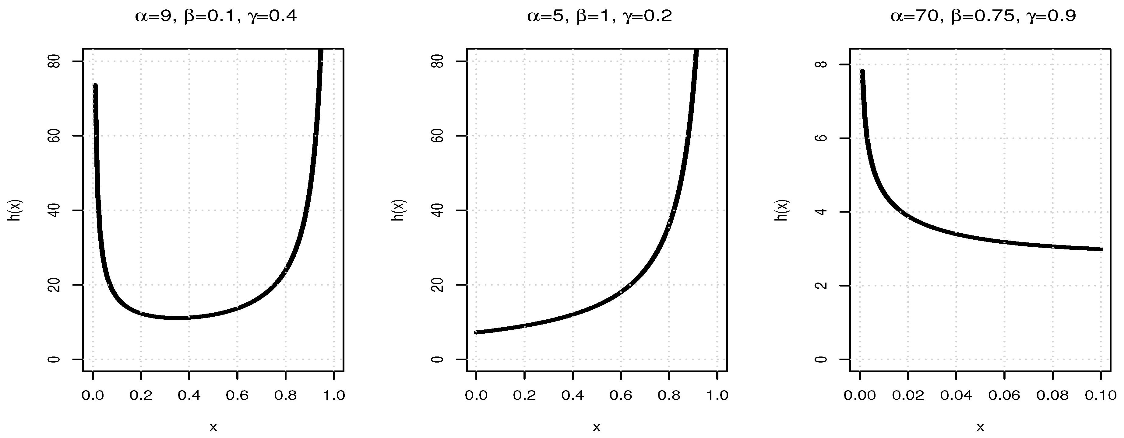
  • The proposed model allows for a wide range of hazard rate forms, such as increasing, decreasing, unimodal, and bathtub.
  • The proposed UJD provides a closed-form CDF and is mathematically tractable, enabling effective computational and analytical processes.
  • It improves data fitting performance for complex and heavily skewed datasets by providing greater control over the behavior of the tails.
The rest of the paper is as follows: Section 2 presents the model formulation, including CDF, PDF, HRF, and graphical illustrations. Section 3 is focused on the UJD and some of its properties, including its quantile function, moments, moment-generating function, order statistics, mean deviation, Bonferroni and Lorenz curves, and entropy. Section 4 shows the parameter estimation. Simulation analysis is examined in Section 5. Real data applications are provided in Section 6. Finally, Section 7 is devoted to some concluding remarks.

2. Probability and Cumulative Distribution Functions

The cumulative distribution function (CDF) of the distribution, as proposed in Alotaibi et al. [34], is expressed as
F x = 1 2 log 1 x log 1 γ α , x 0 , 1 ,
where α > 0 is the shape parameter, and γ 0 , 1 is the median parameter.
An enhanced version of the CDF, which generalizes the model by incorporating an additional parameter β > 0 , called the Unit Jamal Distribution (UJD), is given by
F x = 1 α log 1 x β log 1 γ = 1 1 x β log α log 1 γ , x 0 , 1 ,
where α > 0 , β > 0 , and γ 0 , 1 remains the median parameter.
The corresponding probability density function (PDF) is
f x = β log α x β 1 x β 1 log 1 γ α log 1 x β log 1 γ = β log α log 1 γ x β 1 1 x β 1 log α log 1 γ .
This formulation highlights the direct influence of parameters α , β , and γ on the distribution’s shape and scale.
The hazard rate function (HRF), an essential tool for reliability and survival analysis, is derived as
h x = β log α x β 1 x β 1 log 1 γ .
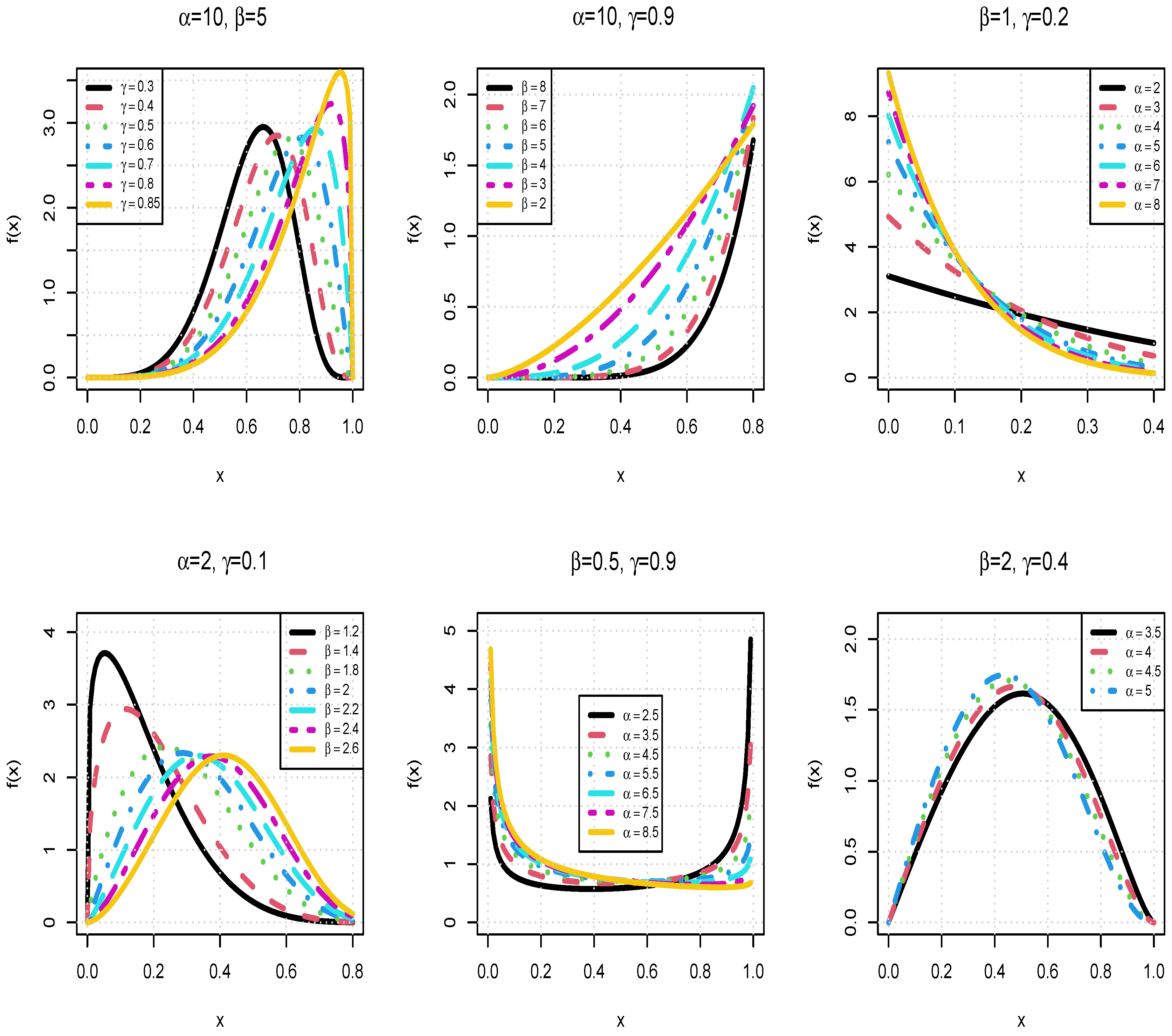
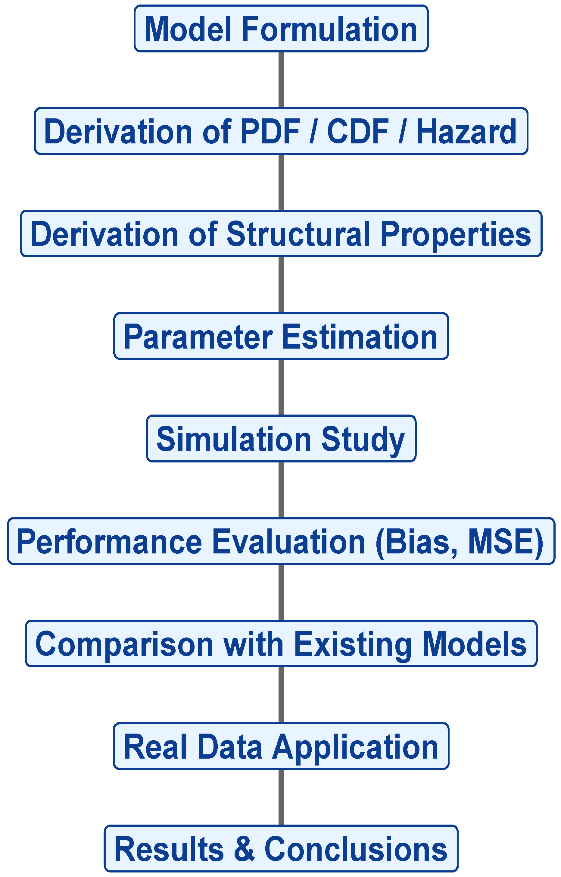
Figure 1 and Figure 2 provide a graphic illustration of PDFs and HRFs for different combinations of α , β , and γ . Figure 3 displays a proposed model flowchart and paper presentation.

3. Properties of the UJD Distribution

3.1. Quantile Function

The quantile function Q u , the inverse of the CDF, provides insight into the percentiles of the distribution. For the UJD distribution, it is expressed as
Q u = 1 1 u log 1 γ log α 1 β , 0 u 1 .
This closed-form representation facilitates the computation of quartiles by substituting u = 0.25 , u = 0.50 , and u = 0.75 for the first, second (median), and third quartiles, respectively. Moreover, the quantile function enables efficient random variate generation, a critical step in simulation studies.

3.2. Moments and Moment Generating Function

The rth ordinary moment of the UJD distribution, denoted as μ r , is given by
μ r = 0 1 x r f ( x ) d x = β log α log 1 γ 0 1 x β + r 1 1 x β 1 log α log 1 γ d x .
After substituting u = x β , the integral becomes
μ r = log α log 1 γ B r β + 1 , log α log 1 γ ,
where B a , b represents the Beta function, defined as B a , b = Γ a Γ b Γ a + b , with Γ . denoting the Gamma function. Substituting this relation, we obtain
μ r = log α log 1 γ Γ r β + 1 Γ log α log 1 γ Γ r β log α log 1 γ + 1 , α > 1 .
The incomplete moments, useful for conditional expectations, are computed as
m r t = 0 t x r f ( x ) d x = β log α log 1 γ 0 t x β + r 1 1 x β log α log 1 γ 1 d x .
After substituting u = x β , and simplifying the integral change into
m r t = β log α t β + r β + r log 1 γ F 1 2 log α log 1 γ + 1 , r β + 1 ; r β + 2 ; t β ,
F 1 2 a , b ; c ; x becomes the hypergeometric function.
The moment generating function (MGF) of X using the relation M X ( t ) = n = 0 t n n ! μ n is given by
M X ( t ) = log α log 1 γ n = 0 Γ n β + 1 Γ log α log 1 γ t n Γ n β log α log 1 γ + 1 n ! , α > 1 .
When r is an integer, the rth central moments of X can be expressed as
μ r = m = 0 r r m μ 1 m μ r m .
The rth cumulants, denoted as κ r of X, can be obtained using the equation
κ r = μ r m = 1 r 1 r 1 m 1 κ m μ r m with κ 1 = μ 1 .

3.3. Skewness and Kurtosis

The skewness and kurtosis provide insights into the distribution’s asymmetry and tail behavior, respectively. The skewness γ 1 is given by
γ 1 = μ 3 μ 2 3 / 2 = κ 3 κ 2 3 / 2 .
The normalized kurtosis γ 2 and non-normalized kurtosis β 2 are expressed as
γ 2 = μ 4 3 μ 2 2 μ 2 2 = κ 4 κ 2 2 , β 2 = μ 4 μ 2 2 = γ 2 3 .
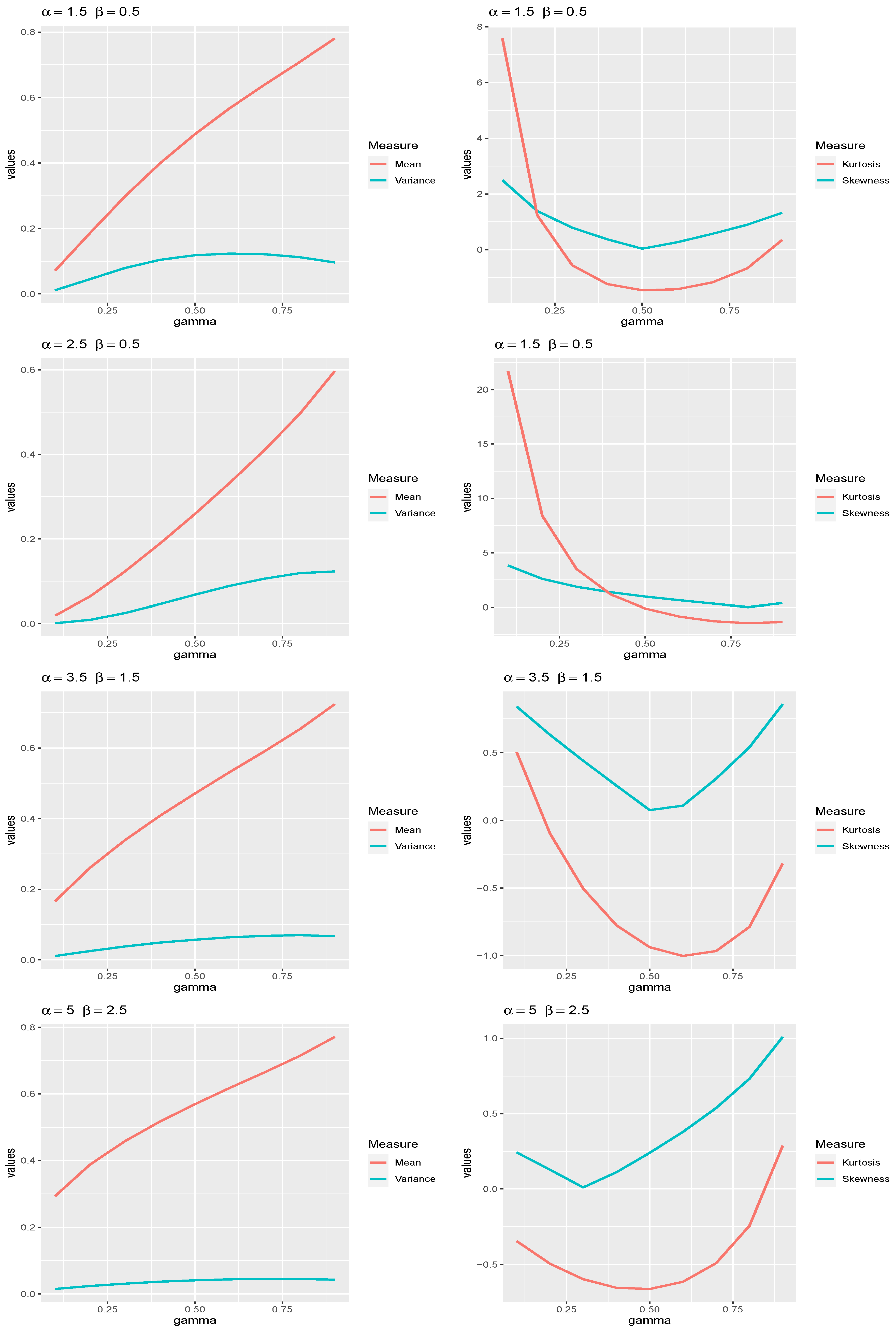
Table 1 provides an in-depth examination of how model parameters impact the mean, variance, skewness, and kurtosis of the UJD model. The findings demonstrate a shift from highly skewed and heavy-tailed behavior to more symmetric and light-tailed behavior as γ increases, shifting the distribution toward higher values and decreasing skewness and kurtosis. By regulating dispersion and shape features, parameters α and β further improve flexibility. Figure 4 further supports the numerical findings reported in Table 1.

3.4. Mean Deviation, Bonferroni Curve, and Lorenz Curve

Let X be a random variable from the UJD distribution, with μ representing its mean and M its median. The mean deviation about the mean, δ 1 X , and about the median, δ 2 X , quantify the average deviation of the random variable from these central measures. They are defined as follows
δ 1 X = 2 μ F μ 2 0 μ x f ( x ) d x , δ 2 X = μ 2 0 M x f ( x ) d x .
For the UJD distribution, these expressions become
δ 1 X = 2 μ 2 μ 1 μ β log α log 1 γ + 2 β log α μ β + 1 β + 1 log 1 γ F 1 2 log α log 1 γ + 1 , 1 β + 1 ; 1 β + 2 ; μ β ,
and
δ 2 X = μ + 2 β log α M β + 1 β + 1 log 1 γ F 1 2 log α log 1 γ + 1 , 1 β + 1 ; 1 β + 2 ; M β ,
where F 1 2 a , b ; c ; x is the hypergeometric function. The Bonferroni and Lorenz curves are key tools in economic and income inequality studies, representing proportional income share distributions. The Bonferroni and Lorenz curves are, respectively, defined as
B F x = 1 μ F x 0 q x f x d x , L F x = 1 F x 0 q x f x d x .
For the UJD distribution, these curves are expressed as
B F x = β log α q β + 1 μ F x β + 1 log 1 γ F 1 2 log α log 1 γ + 1 , 1 β + 1 ; 1 β + 2 ; q β ,
and
L F x = β log α q β + 1 F x β + 1 log 1 γ F 1 2 log α log 1 γ + 1 , 1 β + 1 ; 1 β + 2 ; q β .
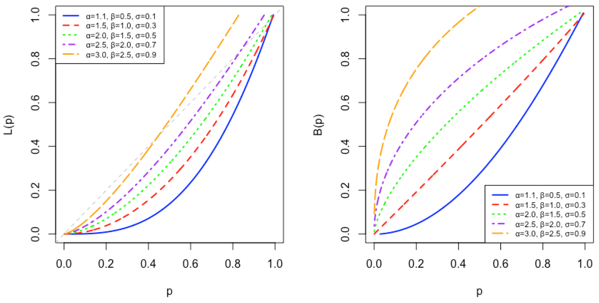
These expressions underscore the flexibility of the UJD distribution in modeling deviations and income distributions, making it suitable for diverse applications in reliability analysis and economics. A graphic representation of the Lorenz and Bonferroni curves with different parameters is provided in Figure 5.

3.5. Order Statistics

Consider a random sample X 1 , X 2 , , X n drawn from the UJD distribution. The probability density function (PDF) of the i-th order statistic, denoted by X i : n , describes the distribution of the i-th smallest value in the sample. The general form of the PDF for X i : n is given by
f i : n ( x ) = n ! f x i 1 ! n i ! j = 0 n i 1 j n i j F x i + j 1 .
Substituting f x and F x for the UJD distribution into this expression, we obtain
f i : n ( x ) = n ! β log α log 1 γ i 1 ! n i ! j = 0 n i 1 j n i j x β 1 1 x β 1 log α log 1 γ × 1 1 x β log α log 1 γ i + j 1 .
Next, applying the binomial expansion to the term 1 1 x β log α log 1 γ i + j 1 , we get
1 1 x β log α log 1 γ i + j 1 = k = 0 i + j 1 k 1 k 1 x β k log α log 1 γ .
Now, applying another binomial expansion to the term 1 x β 1 k + 1 log α log 1 γ , we have
1 x β 1 k + 1 log α log 1 γ = l = 0 1 k + 1 log α log 1 γ l 1 l x β l .
Finally, combining all these expansions, the expression for the PDF of the i-th order statistic is
f i : n ( x ) = n ! β log α log 1 γ i 1 ! n i ! j = 0 n i k = 0 l = 0 1 j + k + l n i j i + j 1 k × 1 k + 1 log α log 1 γ l x l + 1 β 1 .

3.6. Entropy

This subsection examines uncertainty measures within the proposed model by analyzing two widely used entropy measures: Shannon entropy and Rényi entropy. Rényi entropy serves as a generalization of Shannon entropy, and we focus on its derivation for the UJD distribution. The Rényi entropy is mathematically defined as
I R ( ν ) = 1 1 ν log 0 1 f ν ( x ) d x , ν 1 , ν > 0 .
For the UJD distribution, f ν ( x ) is expressed as
f ν ( x ) = β log α log 1 γ ν x β 1 ν 1 x β 1 + log α log 1 γ ν .
To simplify the integral 0 1 f ν ( x ) d x , we perform the substitution u = x β , which transforms the integral and limits accordingly. After the substitution, the integral can be expressed in terms of the Beta function, B ( a , b ) , as
f ν ( x ) = 1 β β log α log 1 γ ν B 1 + β 1 ν β , 1 ν ν log α log 1 γ .
The RE for the UJD distribution is as follows:
I R ( ν ) = 1 1 ν log 1 β β log α log 1 γ ν B 1 + β 1 ν β , 1 ν ν log α log 1 γ ,
where α > 1 , ν 1 , ν > 0 . The Havrda and Charvat (HC) entropy for the UJD distribution is as follows:
I H C ( ν ) = 1 2 1 ν 1 1 β β log α log 1 γ ν B 1 + β 1 ν β , 1 ν ν log α log 1 γ 1 .

3.7. Entropy-Based Relative Loss

Let W ( X ) be an entropy and W p ( Y ) be its truncated integral version at p, i.e., defined with the truncated version of f ( y ) over the interval ( 0 , p ) . Then we define the corresponding entropy-based relative loss (RL) as follows:
S W ( p ) = W ( X ) W p ( Y ) W ( X ) ,
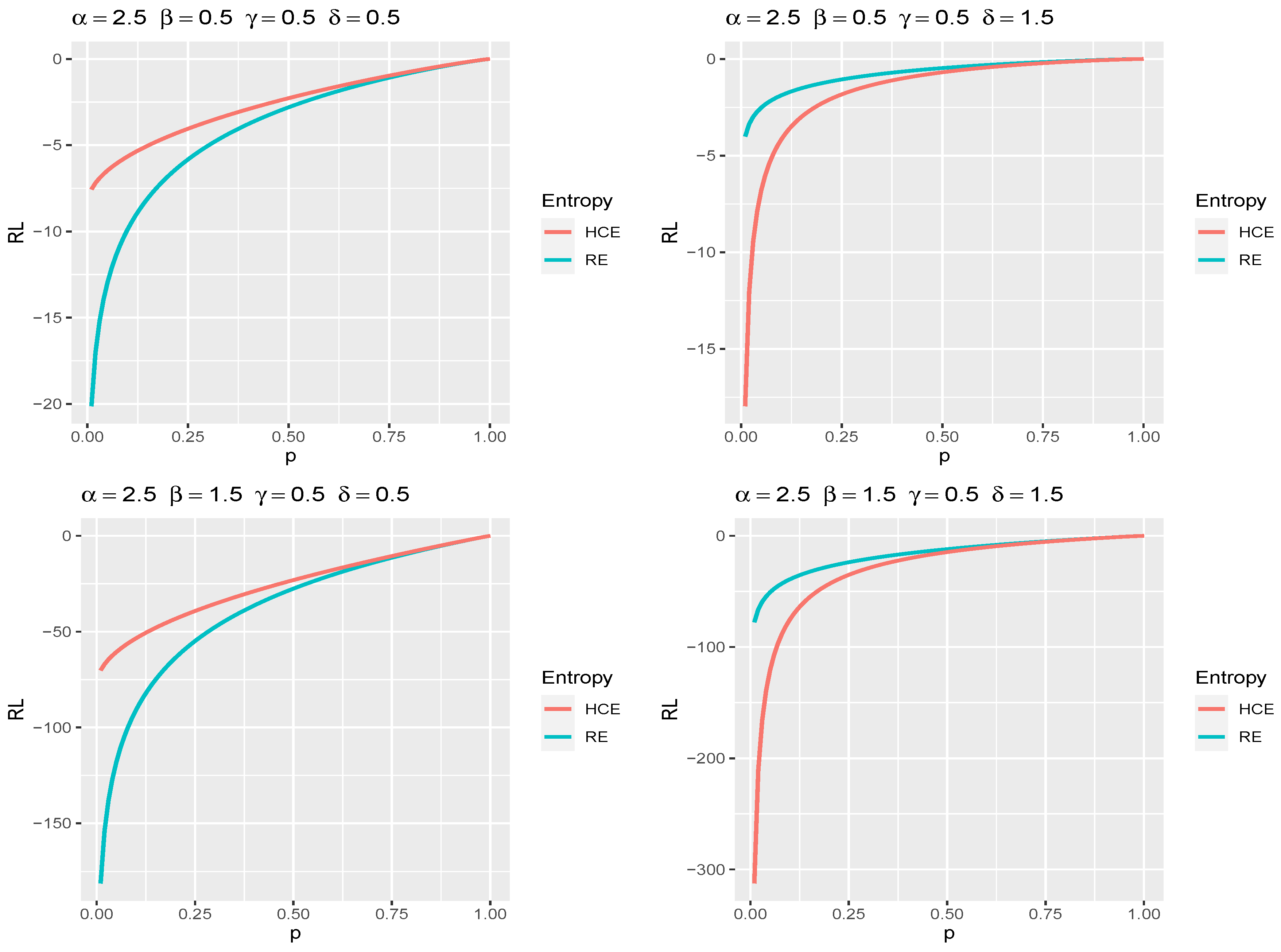
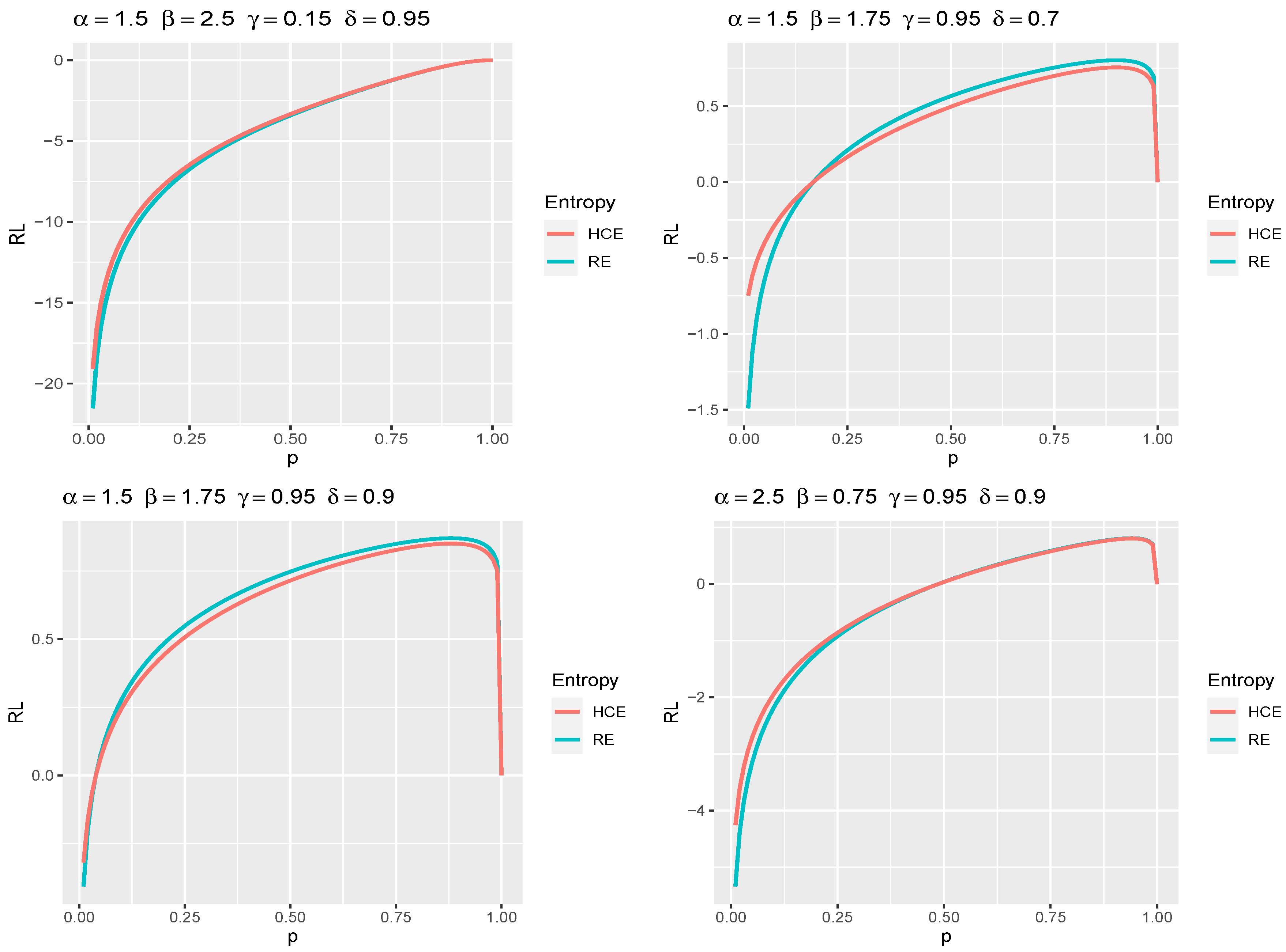
for RE, W p ( Y ) = 1 1 ν log 0 p f t ( y ) ν d y , the truncated PDF can be obtained f t ( y ) = f ( y ) / F ( p ) . The F ( p ) and f ( y ) are defined in Equations (1) and (2), respectively. Figure 6 presents a visual representation of the RL based on RE and HCE for selected parameter values of the UJD model. The relative entropy loss decreases with increasing truncation time p, indicating improved information retention.

4. Maximum Likelihood Estimation

The Maximum Likelihood Estimation (MLE) method is used to estimate the parameters of the UJD distribution. Let X 1 , X 2 , , X n represent a random sample of size n with observed values x 1 , x 2 , , x n . The distribution is defined by three parameters: α , β , and γ .
  • The log-likelihood function for the UJD distribution, based on the observed sample, is
    l ( α , β , γ ) = n log β log α log 1 γ + β 1 i = 1 n log x i 1 + log α log 1 γ i = 1 n log 1 x i β .
To find the maximum likelihood estimates (MLEs) for these parameters, we compute the partial derivatives of the log-likelihood function with respect to each parameter and set them equal to zero. This yields a system of nonlinear equations that must be solved simultaneously. The derivatives are given as follows:
l α = n α log α i = 1 n log 1 x i β α log 1 γ ,
l β = n β + i = 1 n log x i + 1 + log α log 1 γ i = 1 n x i β log x i 1 x i β ,
l γ = 1 1 γ log 1 γ n log α log 1 γ i = 1 n log 1 x i β .
The parameters α ^ , β ^ , and γ ^ , which maximize the log-likelihood function, are the MLEs for α , β , and γ , respectively. However, since the equations above are nonlinear, no closed-form solutions exist for direct computation. Instead, numerical optimization techniques are used to solve this system.
Let ζ = ( α , β , γ ) denote the parameter vector of the UJD model, where α > 0 , β > 0 , and 0 < γ < 1 . For a random sample x 1 , x 2 , , x n , the likelihood function is given by
L ( ζ ) = i = 1 n f ( x i ζ ) ,
and the corresponding log-likelihood function is given in Equation (11). We assume the following independent prior distributions: α Gamma ( a 1 , b 1 ) , β Gamma ( a 2 , b 2 ) , and γ Beta ( c 1 , c 2 ) . Using Bayes theorem, the joint posterior distribution is given by
π ( ζ x ) L ( ζ ) π ( α ) π ( β ) π ( γ ) .
Since the posterior distribution does not have a closed form, we generate samples from it using the Metropolis–Hastings algorithm (MHA). Samples from the posterior distribution of the parameters α , β , and γ are produced using the MHA. First, the initial values α ( 0 ) , β ( 0 ) , and γ ( 0 ) are chosen. While maintaining the parameter constraints α > 0 , β > 0 , and 0 < γ < 1 , candidate values α * , β * , and γ * are generated at each iteration t from normal proposal distributions centered at the current states with variances σ α 2 , σ β 2 , and σ γ 2 , respectively. The proposed values are then accepted with probability
A = min 1 , π ( α * , β * , γ * x ) π ( α ( t ) , β ( t ) , γ ( t ) x ) ,
otherwise, the values remain unchanged. This procedure is repeated for a sufficient number of iterations M in order to get posterior samples. For further details regarding the MHA, see [15].

5. Simulation

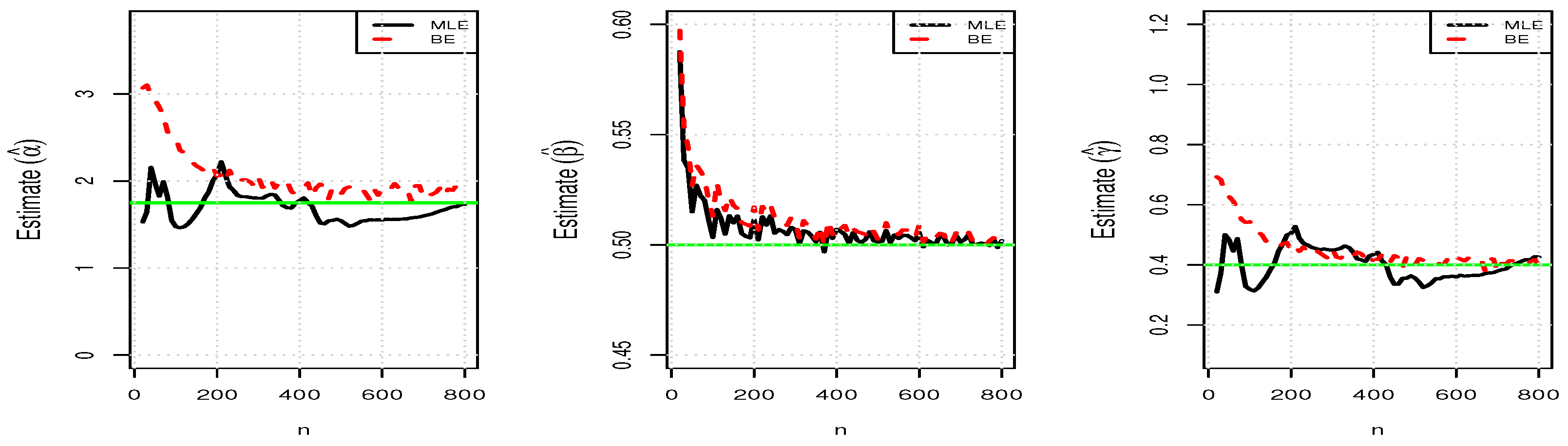
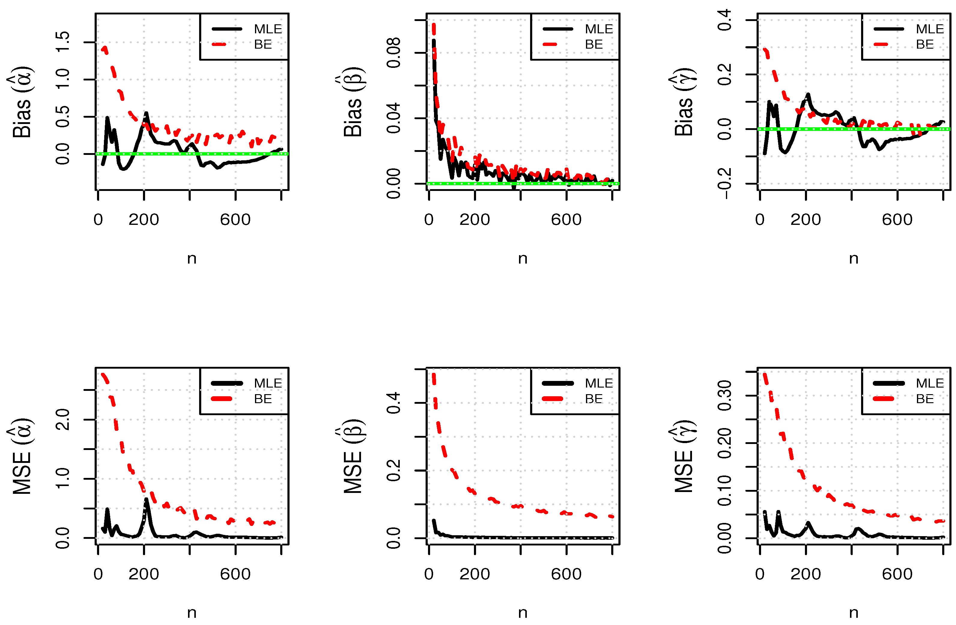
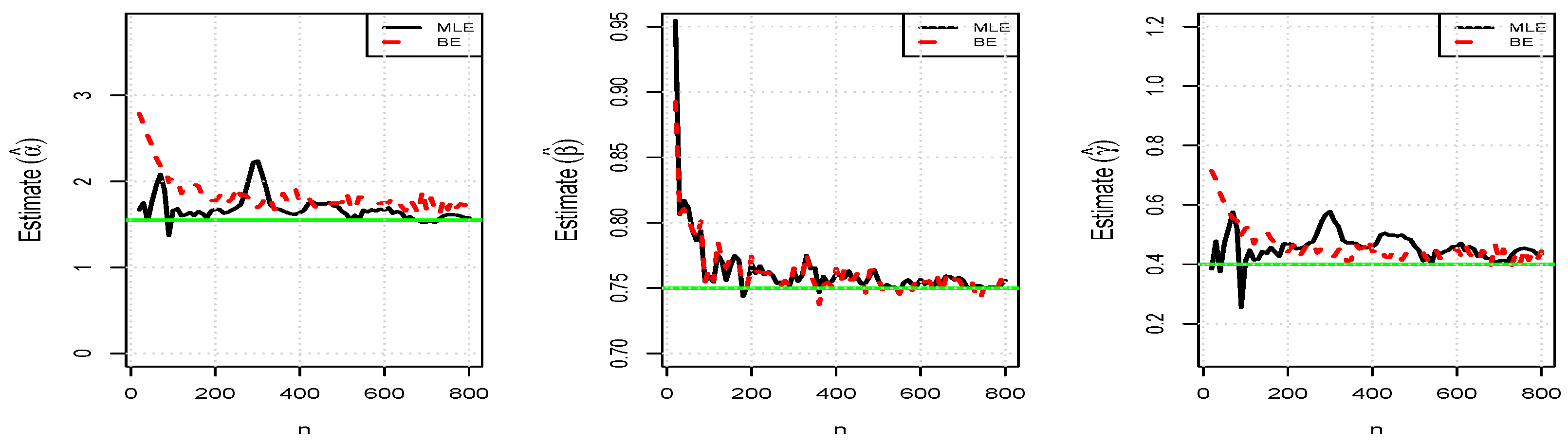
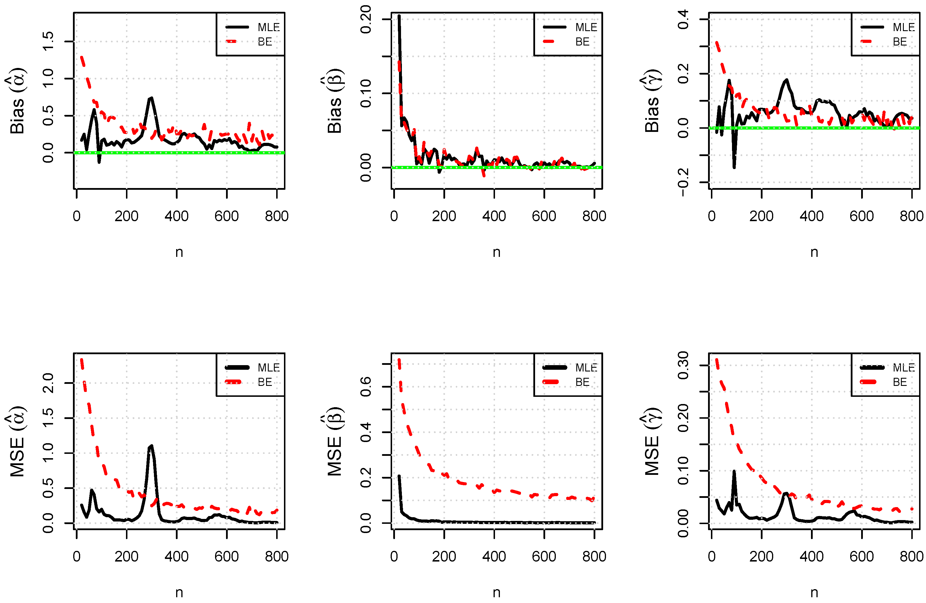
The performance of two estimation techniques, namely, maximum likelihood estimation (MLE) and Bayesian estimation (BE), is highlighted in this section through a simulation study. A range of sample sizes ( n = 50 , 60 , , 800 ) is taken into consideration to illustrate the relationships between n and estimation consistency. The calculation of biases and mean square errors (MSEs) is performed after getting N = 1000 replications per n. For BE, we use N = 1000 iterations and the first 30% as a burn-in sample. Two parametric combinations are used as follows: α ( 1.50 , 1.67 ) , β ( 0.50 , 0.75 ) , and λ = 0.40 . We use the BFGS (Broyden Fletcher Goldfarb Shanno) algorithm, a quasi-Newton method for smooth nonlinear optimization problems, particularly maximum likelihood estimation [35]. For BE, the Markov Chain Monte Carlo (MCMC) process is initiated considering the MLEs; the proposal distributions have been modified so that their standard deviations are 15% of the corresponding MLE estimates. Overall, the simulation study’s results demonstrated that as n increases, biases and MSEs decrease under both estimate methodologies (as shown in Figure 7, Figure 8, Figure 9 and Figure 10). The average estimates (AEs) approach parametric true values as n increases (as shown in Figure 7, Figure 8 and Figure 9). The process used to carry out a Monte Carlo simulation is as follows:
(i)
Set the initial values of the parameters α , β , γ ;
(ii)
Draw a random sample of size n using the QF given in Equation (4); we consider a various n such as 50, 60, …, 800;
(iii)
Next, we compute the AEs, biases, and MSE of the estimates considering the following formulas:
AE ( ω ^ ) = i = 1 1000 ω i ^ 1000 , MSE ( ω ^ ) = i = 1 1000 ( ω i ^ ω ) 2 1000 , Bias ( ω ^ ) = i = 1 1000 ω i ^ 1000 ω ,
respectively, (for ω = α , β , γ );
(iv)
Do N = 1000 times replications of steps (ii) and (iii).

6. Applications

This section is based on the real data application of the proposed model to underscore its usefulness and relevance in practical scenarios. To this end, we use a real data sets to demonstrate the performance of the UJD model against several other unit interval-based models. We compare two data sets with some of the most well-known unit interval models, including the unit Burr-XII (UBXII) model [30], the Poisson unit Weibull (PUW) model [15], the unit Weibull (UW) model [7], and the unit half logistic-geometric (UFLG) [33].

6.1. First Dataset

The first dataset ( D I ) is one of the failure times from 50 electronic devices, and it was recently used by Al-Essa et al. [36]. Table 2 provides the first data:

6.2. Second Dataset

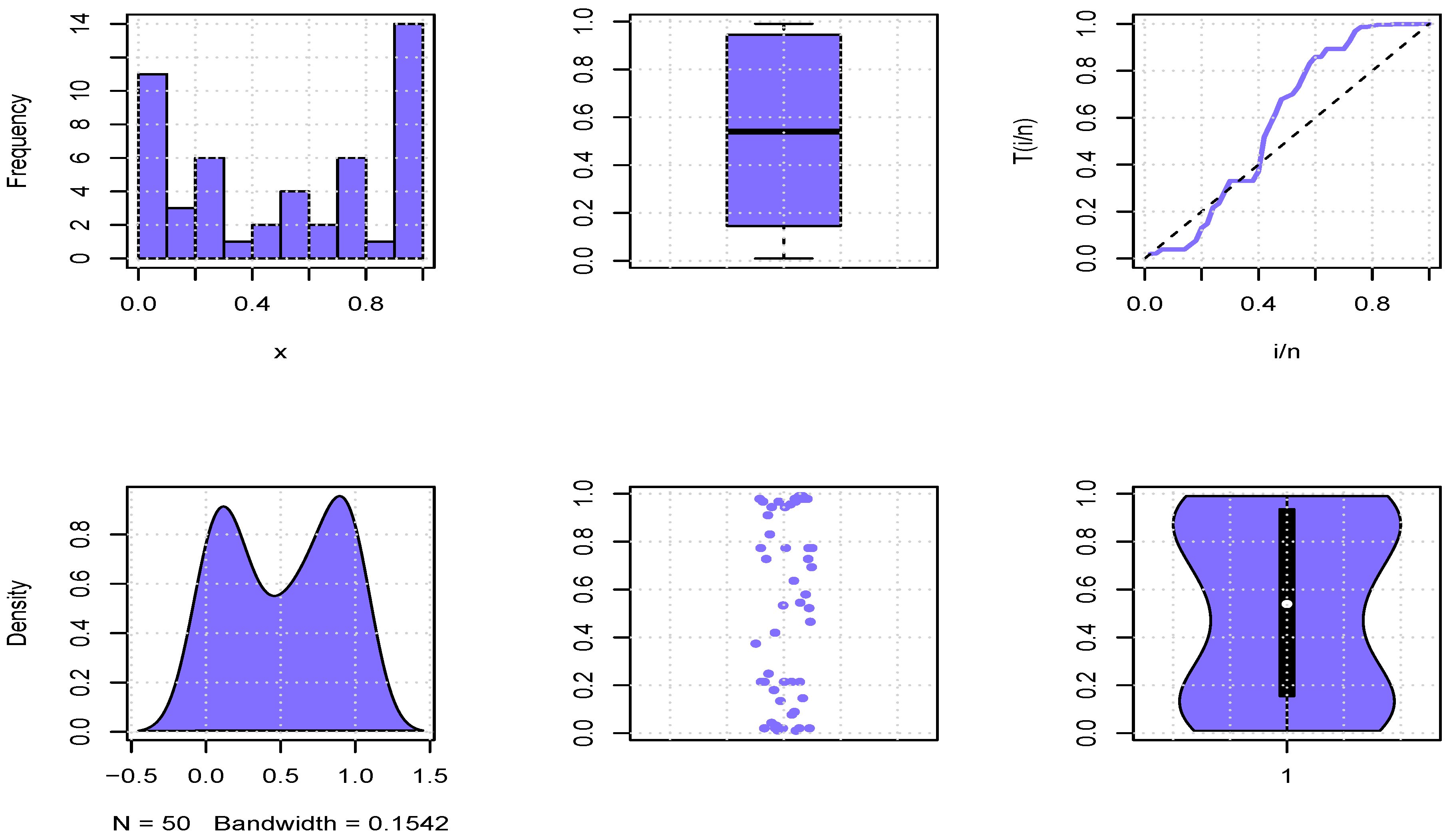
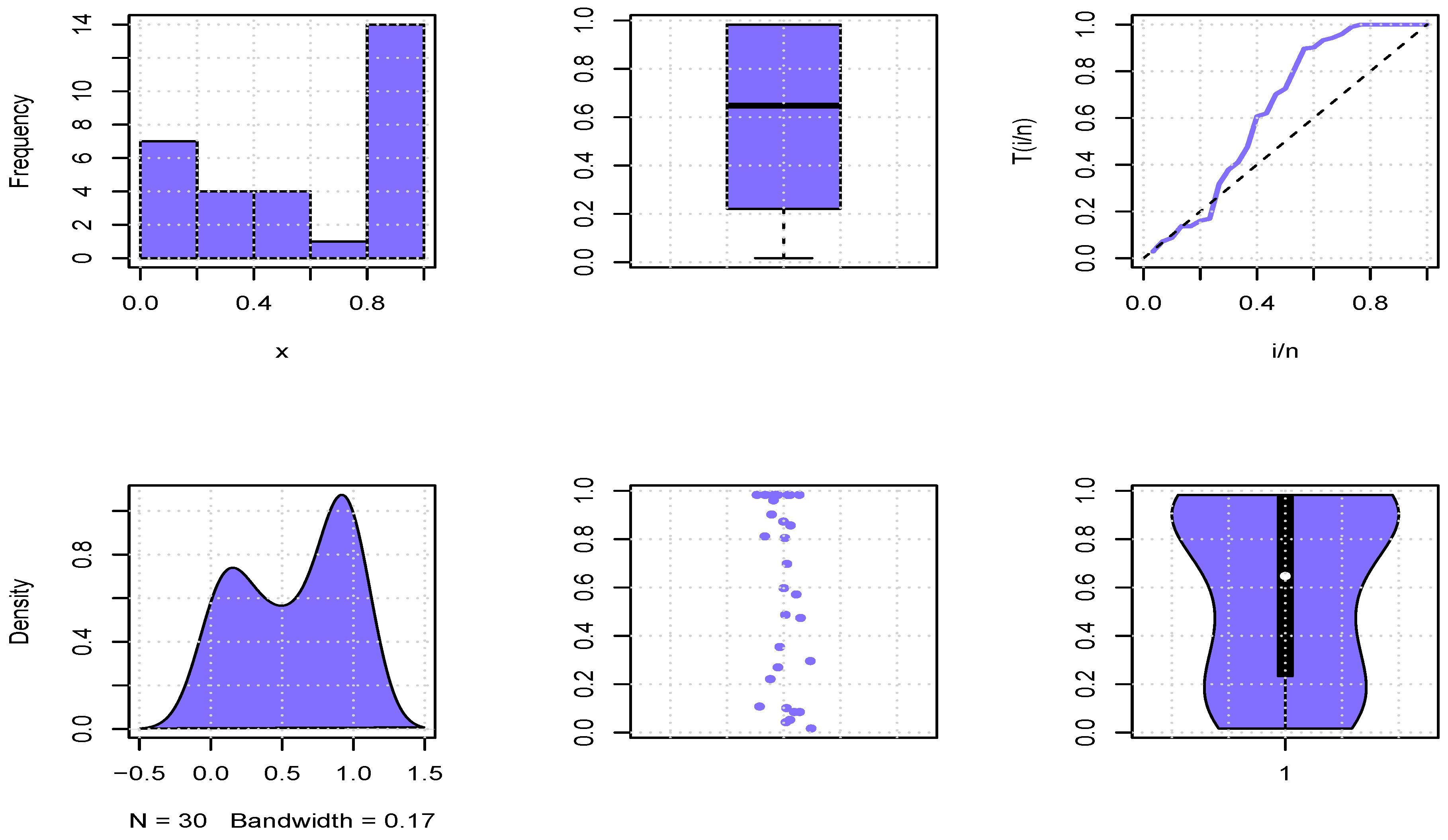
The second dataset ( D II ) consists of the lifetime duration of 30 electronic components taken from power-line voltage spikes during electric storms. Recently, Muhammad et al. [15] analyzed the data using the PUW model. Moreover, D II has the bathtub shape as shown in histogram in Figure 11. Table 3 presents the second dataset:
Figure 12 graphically presents the second dataset.

6.3. Third Dataset

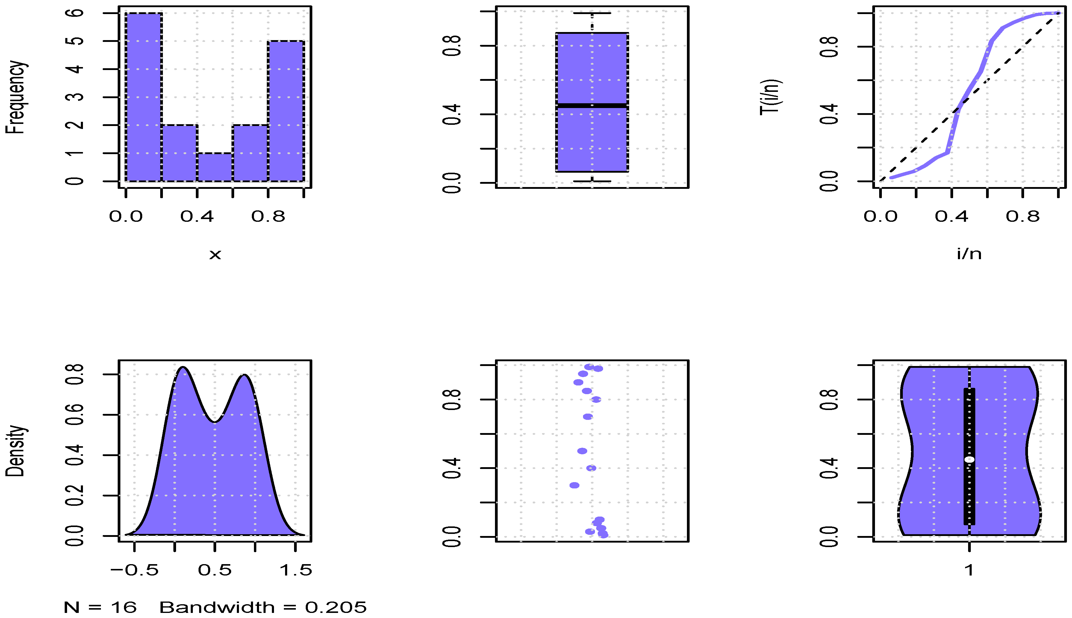
Table 4 presents the simulated data generated using the quantile function of the UJD model. The dataset consists of 16 observations.
The second dataset is shown graphically in Figure 13.
Table 5 demonstrates that all datasets have comparable dispersion and variability. A moderate asymmetry in the data is shown by the skewness. The datasets are suitable for bounded distribution modeling since the kurtosis values indicate light-tailed behavior.
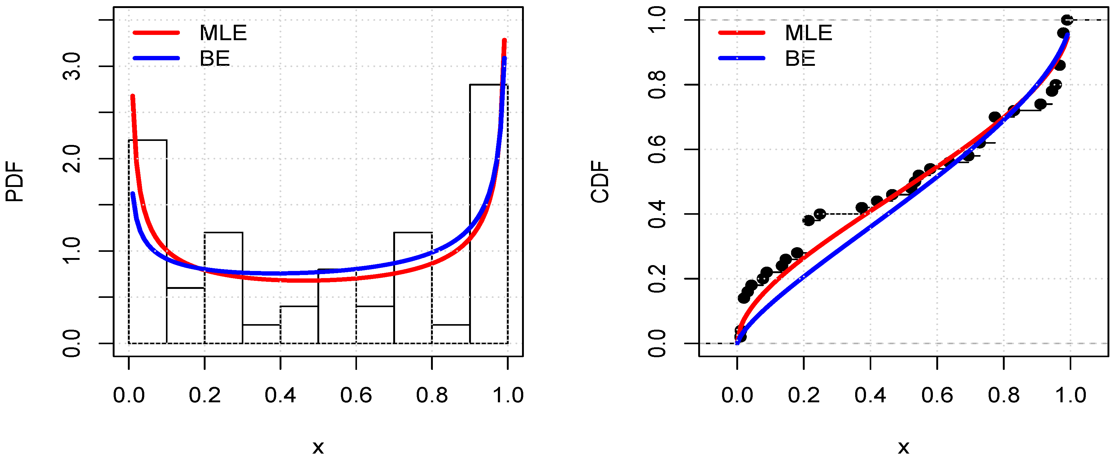
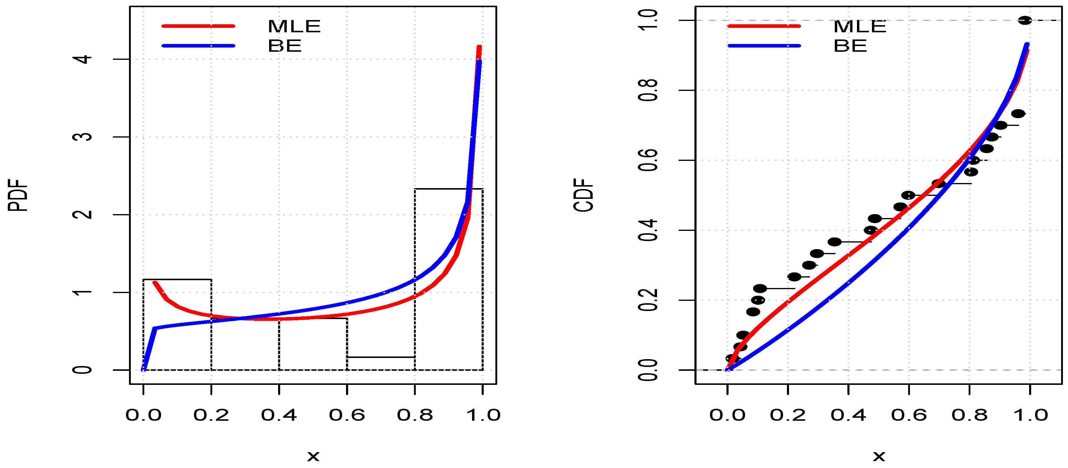
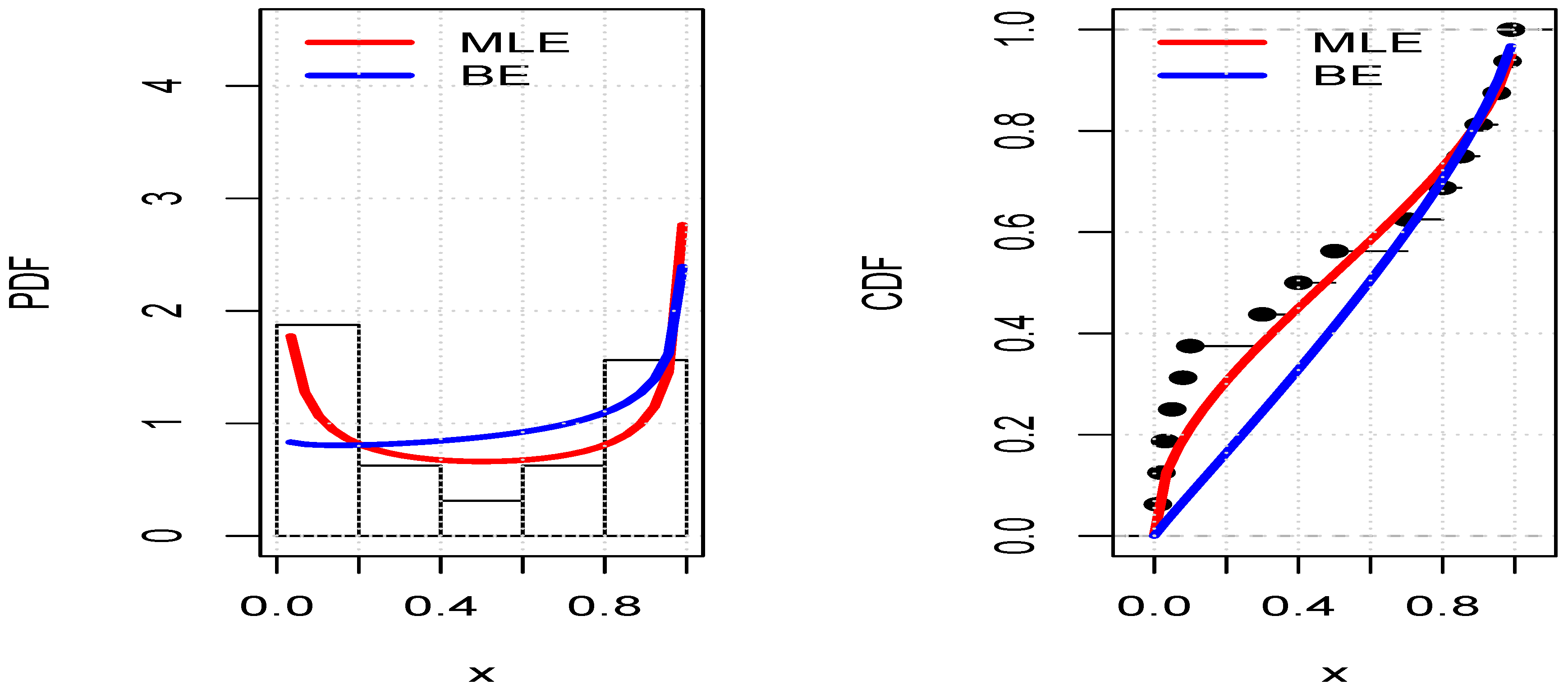
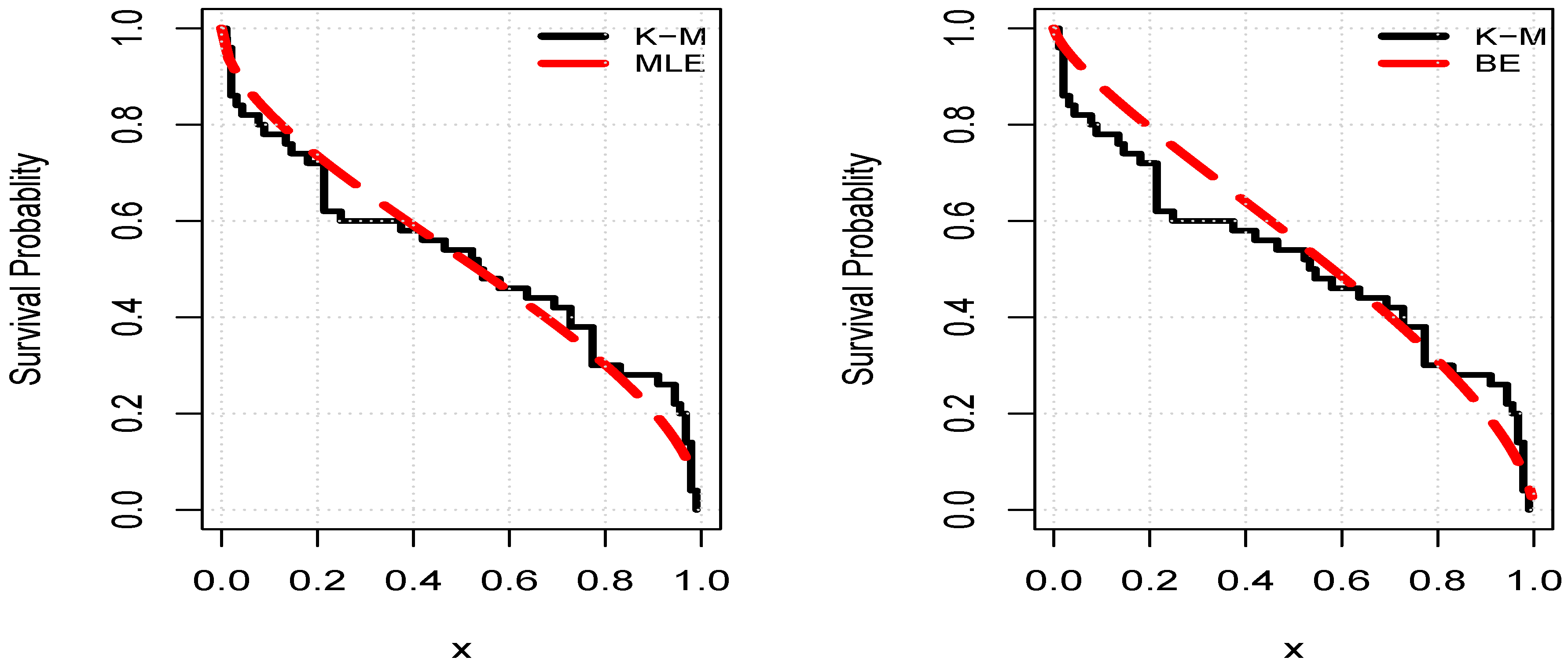
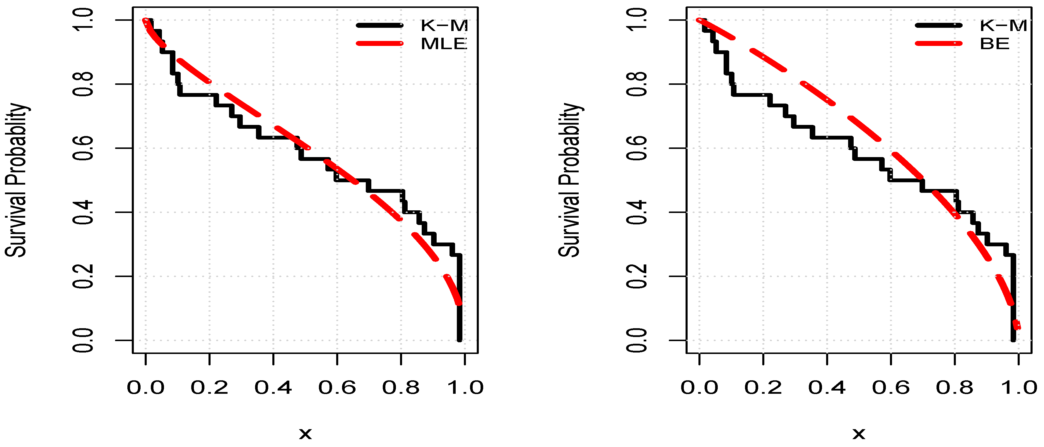
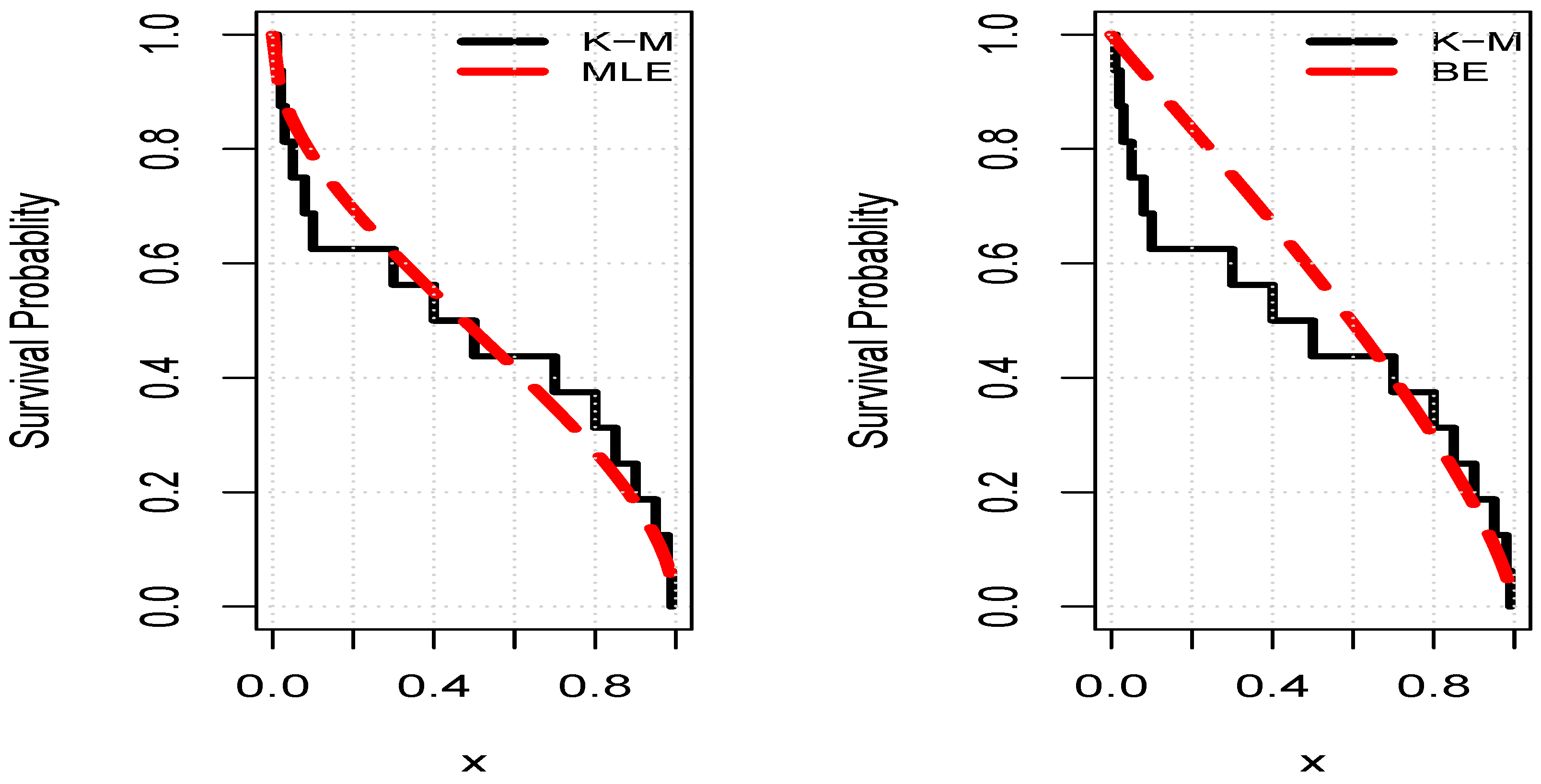
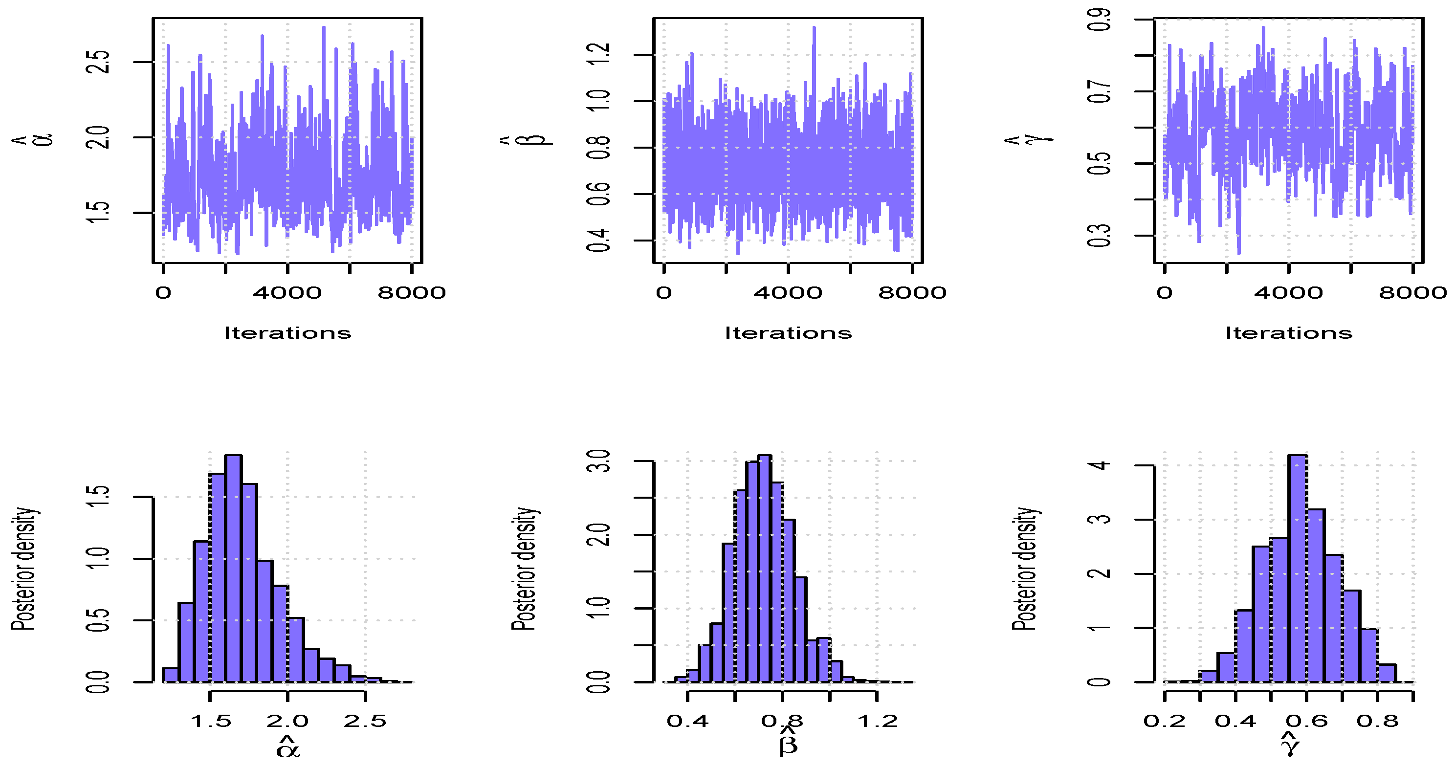
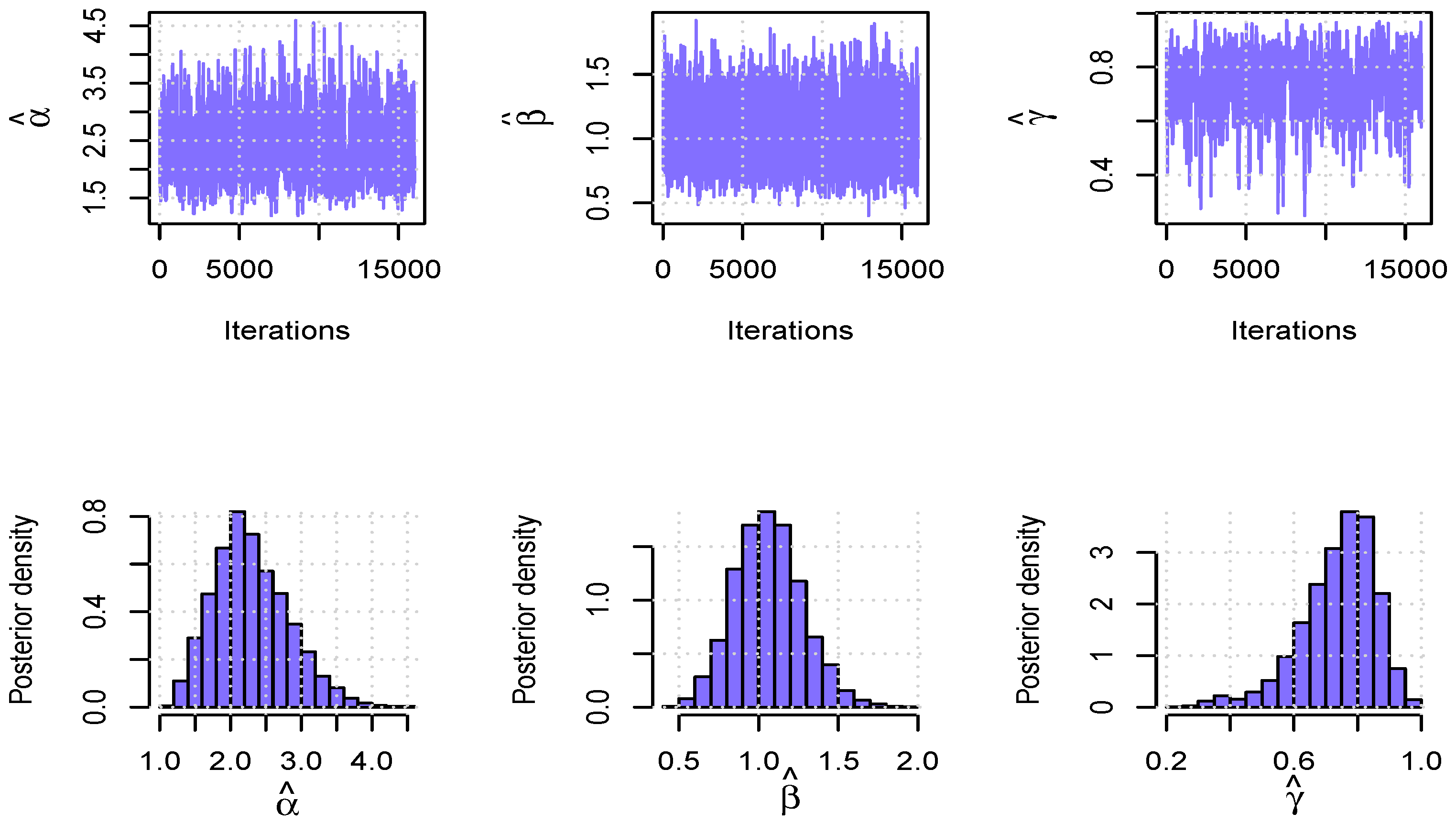
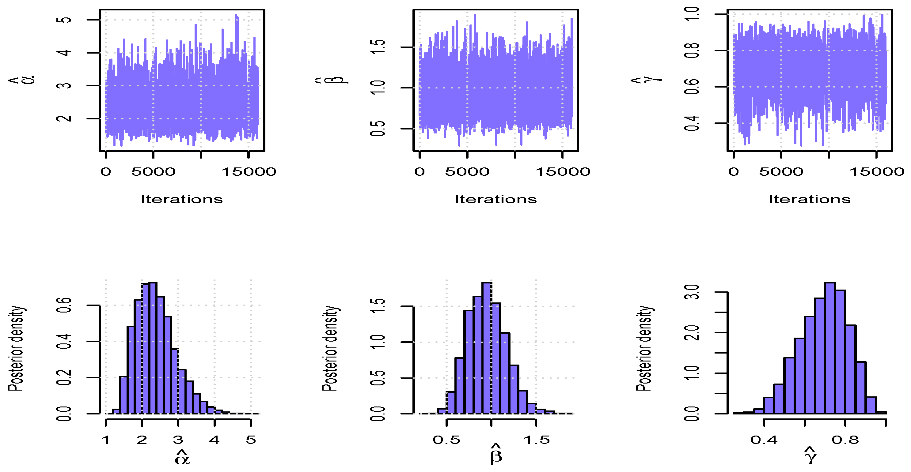
The competing models are compared in Table 6 with respect to log-likelihood (LL), Anderson–Darling (AD), Cramér–von Mises (CVM), Kolmogorov–Smirnov (KS), and p-value (PV). A better model fit is indicated by lower AD and CVM values as well as a higher KS p-value. Table 7 displays the Bayesian estimation with 95% lower and upper credible intervals for each data set. While Table 8 provides the Kolmogorov–Smirnov test using the Bayesian estimation. The maximum likelihood estimates perform better compared to the Bayesian estimates. A graphical illustration of the estimated PDF and CDF for the UJD model, based on both MLE and Bayesian estimation across all datasets, is presented in Figure 14, Figure 15 and Figure 16. A graphical illustration of the K–M plots based on both estimation methods for all three datasets is presented in Figure 17, Figure 18 and Figure 19. A graphical representation of the iterations (top) and posterior PDFs (bottom) for α ^ , β ^ , and γ ^ , based on the UJD model using the HM algorithm and Gibbs sampling across all datasets, is presented in Figure 20, Figure 21 and Figure 22. These illustrations show the effectiveness and suitability of the proposed paradigm for modeling and assessing real data.

7. Concluding Remarks

This paper introduced the unit Jamal distribution (UJD), a flexible model for data on the (0, 1) interval. We explored its theoretical properties, derived key statistical measures, and estimated parameters using the maximum likelihood method. The simulation results confirmed the efficiency of the estimators, and real data applications showed that the UJD provides a better fit than several existing models. Overall, the UJD is a valuable addition to the family of unit distributions, offering improved flexibility for modeling real data sets. Moreover, the proposed distribution can be extended to quantile regression analysis due to the availability of a closed-form quantile function.

Author Contributions

F.J. contributed to conceptualization and methodology; M.A.A.E. performed data analysis and evaluated results; M.I. designed simulation and Bayesian analysis; and S.M. derived distributional properties and contributed to review and editing of the manuscript. All authors have read and agreed to the published version of the manuscript.

Funding

This work was supported and funded by the Deanship of Scientific Research at Imam Mohammad Ibn Saud Islamic University (IMSIU) (grant number IMSIU-DDRSP2601).

Data Availability Statement

All datasets analyzed during this study are included within the article.

Conflicts of Interest

The authors declare no competing interests.

References

  1. Gómez-Déniz, E.; Sordo, M.A.; Calderín-Ojeda, E. The Log–Lindley distribution as an alternative to the beta regression model with applications in insurance. Insur. Math. Econ. 2014, 54, 49–57. [Google Scholar] [CrossRef]
  2. Mazucheli, J.; Menezes, A.F.; Dey, S. The unit-Birnbaum-Saunders distribution with applications. Chil. J. Stat. 2018, 9, 47–57. [Google Scholar]
  3. Ghitany, M.E.; Mazucheli, J.; Menezes, A.F.B.; Alqallaf, F. The unit-inverse Gaussian distribution: A new alternative to two-parameter distributions on the unit interval. Commun. Stat.-Theory Methods 2019, 48, 3423–3438. [Google Scholar] [CrossRef]
  4. Altun, E.; Cordeiro, G.M. The unit-improved second-degree Lindley distribution: Inference and regression modeling. Comput. Stat. 2020, 35, 259–279. [Google Scholar] [CrossRef]
  5. Guerra, R.R.; Peña-Ramírez, F.A.; Bourguignon, M. The unit extended Weibull families of distributions and its applications. J. Appl. Stat. 2021, 48, 3174–3192. [Google Scholar] [CrossRef] [PubMed]
  6. Consul, P.C.; Jain, G.C. On the log-gamma distribution and its properties. Stat. Hefte 1971, 12, 100–106. [Google Scholar] [CrossRef]
  7. Mazucheli, J.; Menezes, A.F.B.; Ghitany, M.E. The unit-Weibull distribution and associated inference. J. Appl. Probab. Stat. 2018, 13, 1–22. [Google Scholar]
  8. Mazucheli, J.; Menezes, A.F.; Dey, S. Unit-Gompertz distribution with applications. Statistica 2019, 79, 25–43. [Google Scholar]
  9. Altun, E.; Hamedani, G.G. The log-xgamma distribution with inference and application. J. Société Française Stat. 2018, 159, 40–55. [Google Scholar]
  10. Korkmaz, M.Ç. The unit generalized half normal distribution: A new bounded distribution with inference and application. UPB Sci. Bull. Ser. A 2020, 82, 133–140. [Google Scholar]
  11. Elgarhy, M.; Abdalla, G.S.S.; Hassan, A.S.; Almetwally, E.M. Bayesian and Non-Bayesian Analysis of the Novel Unit Inverse Exponentiated Lomax Distribution Using Progressive Censoring Schemes with Optimal Scheme and Data Application. Comput. J. Math. Stat. Sci. 2025, 5, 78–108. [Google Scholar] [CrossRef]
  12. Muhammad, M.; Sallam Salem Abdalla, G.; Faal, A.; Almetwally, E.M.; Elgarhy, M. A Flexible Approach to Quantile Regression Modeling With Unit Burr-XII-Poisson and Its Applications to Cancer, Chemotherapy, and Energy Data. Eng. Rep. 2025, 7, e70312. [Google Scholar] [CrossRef]
  13. Gemeay, A.M.; Alsadat, N.; Chesneau, C.; Elgarhy, M. Power unit inverse Lindley distribution with different measures of uncertainty, estimation and applications. AIMS Math. 2024, 9, 20976–21024. [Google Scholar] [CrossRef]
  14. Ragab, I.E.; Alsadat, N.; Balogun, O.S.; Elgarhy, M. Unit extended exponential distribution with applications. J. Radiat. Res. Appl. Sci. 2024, 17, 101118. [Google Scholar] [CrossRef]
  15. Muhammad, M.; Abba, B.; Xiao, J.; Alsadat, N.; Jamal, F.; Elgarhy, M. A New Three-Parameter Flexible Unit Distribution and Its Quantile Regression Model. IEEE Access 2024, 12, 156235–156251. [Google Scholar] [CrossRef]
  16. Alghamdi, S.M.; Shrahili, M.; Hassan, A.S.; Elbatal, I.; Amin, E.A.; Elgarhy, M. Analysis of Milk Production and Failure Data: Using Unit Exponentiated Half Logistic Power Series Class of Distributions. Symmetry 2023, 15, 714. [Google Scholar] [CrossRef]
  17. Haj Ahmad, H.; Almetwally, E.M.; Elgarhy, M.; Ramadan, D.A. On Unit Exponential Pareto Distribution for Modeling the Recovery Rate of COVID-19. Processes 2023, 11, 232. [Google Scholar] [CrossRef]
  18. Bantan, R.A.R.; Jamal, F.; Chesneau, C.; Elgarhy, M. Theory and Applications of the Unit Gamma/Gompertz Distribution. Mathematics 2021, 9, 1850. [Google Scholar] [CrossRef]
  19. Bantan, R.A.; Chesneau, C.; Jamal, F.; Elgarhy, M.; Tahir, M.H.; Ali, A.; Zubair, M.; Anam, S. Some New Facts about the Unit-Rayleigh Distribution with Applications. Mathematics 2020, 8, 1954. [Google Scholar] [CrossRef]
  20. Hassan, A.S.; Fayomi, A.; Algarni, A.; Almetwally, E.M. Bayesian and Non-Bayesian Inference for Unit-Exponentiated Half-Logistic Distribution with Data Analysis. Appl. Sci. 2022, 12, 11253. [Google Scholar] [CrossRef]
  21. Altun, E. The log-weighted exponential regression model: Alternative to the beta regression model. Commun. Stat.-Theory Methods 2021, 50, 2306–2321. [Google Scholar] [CrossRef]
  22. Lindley, D.V. Fiducial distributions and Bayes’ theorem. J. R. Stat. Soc. Ser. B (Methodol.) 1958, 20, 102–107. [Google Scholar] [CrossRef]
  23. Sen, S.; Maiti, S.S.; Chandra, N. The xgamma distribution: Statistical properties and application. J. Mod. Appl. Stat. Methods 2016, 15, 38. [Google Scholar] [CrossRef]
  24. Elgarhy, M. Garhy distribution with Different Estimation Methods and Applications to Engineering and Medical Data. Rev. Int. Metod. Numer. Calc. Diseno Ing. 2026, 42, 90. [Google Scholar] [CrossRef]
  25. Cooray, K.; Ananda, M.M. A generalization of the half-normal distribution with applications to lifetime data. Commun. Stat.-Theory Methods 2008, 37, 1323–1337. [Google Scholar] [CrossRef]
  26. Gupta, R.D.; Kundu, D. A new class of weighted exponential distributions. Statistics 2009, 43, 621–634. [Google Scholar] [CrossRef]
  27. Mazucheli, J.; Menezes, A.F.B.; Chakraborty, S. On the one parameter unit-Lindley distribution and its associated regression model for proportion data. J. Appl. Stat. 2019, 46, 700–714. [Google Scholar] [CrossRef]
  28. Korkmaz, M.Ç. A new heavy-tailed distribution defined on the bounded interval: The logit slash distribution and its application. J. Appl. Stat. 2020, 47, 2097–2119. [Google Scholar] [CrossRef] [PubMed]
  29. Gündüz, S.; Korkmaz, M.Ç. A new unit distribution based on the unbounded Johnson distribution rule: The unit Johnson SU distribution. Pak. J. Stat. Oper. 2020, 16, 471–490. [Google Scholar] [CrossRef]
  30. Korkmaz, M.Ç.; Chesneau, C. On the unit Burr-XII distribution with the quantile regression modeling and applications. Comput. Appl. Math. 2021, 40, 29. [Google Scholar] [CrossRef]
  31. Korkmaz, M.Ç.; Chesneau, C.; Korkmaz, Z.S. Transmuted unit Rayleigh quantile regression model: Alternative to beta and Kumaraswamy quantile regression models. Univ. Politeh. Buchar. Sci. Bull. Ser. Appl. Math. Phys. 2021, 83, 149–158. [Google Scholar]
  32. Korkmaz, M.Ç.; Chesneau, C.; Korkmaz, Z.S. On the arcsecant hyperbolic normal distribution. Properties, quantile regression modeling and applications. Symmetry 2021, 13, 117. [Google Scholar] [CrossRef]
  33. Ramadan, A.T.; Tolba, A.H.; El-Desouky, B.S. A unit half-logistic geometric distribution and its application in insurance. Axioms 2022, 11, 676. [Google Scholar] [CrossRef]
  34. Alotaibi, R.; Nassar, M.; Elshahhat, A. Analysis of the new complementary unit Weibull model from adaptive progressively type-II hybrid. AIP Adv. 2024, 14, 045014. [Google Scholar] [CrossRef]
  35. Marinho, P.R.D.; Silva, R.B.; Bourguignon, M.; Cordeiro, G.M.; Nadarajah, S. AdequacyModel: An R package for probability distributions and general purpose optimization. PLoS ONE 2019, 14, e0221487. [Google Scholar] [CrossRef]
  36. Al-Essa, L.A.; Muhammad, M.; Tahir, M.H.; Abba, B.; Xiao, J.; Jamal, F. A new flexible four parameter bathtub curve failure rate model, and its application to right-censored data. IEEE Access 2023, 11, 50130–50144. [Google Scholar] [CrossRef]
Figure 1. A graphic demonstration of PDFs for different combinations of α , β , and γ .
Axioms 15 00359 g001
Figure 2. A graphic demonstration of HRFs for different combinations of α , β , and γ .
Axioms 15 00359 g002
Figure 3. Proposed model flowchart and paper presentation.
Axioms 15 00359 g003
Figure 4. A graphic illustration of the parametric effects on mean, variance, skewness, and kurtosis based on the UJD model.
Axioms 15 00359 g004
Figure 5. Plots of Lorenz and Bonferroni curves with different parameters.
Axioms 15 00359 g005
Figure 6. A visual representation of the RL based on the RE, and HCE for some parametric values of the UJD model.
Axioms 15 00359 g006aAxioms 15 00359 g006b
Figure 7. A graphic demonstration of AEs at varying n for both estimation methods taking α = 1.67 , β = 0.50 , and λ = 0.40 . The green line represents the true parametric value used as a reference in the figure.
Axioms 15 00359 g007
Figure 8. A graphic demonstration of biases and MSEs at varying n for both estimation methods taking α = 1.67 , β = 0.50 , and λ = 0.40 . The green line in the bias plot represents the zero-bias reference line.
Axioms 15 00359 g008
Figure 9. A graphic demonstration of AEs at varying n for both estimation methods taking α = 1.50 , β = 0.75 , and λ = 0.40 . The green line represents the true parametric value used as a reference in the figure.
Axioms 15 00359 g009
Figure 10. A graphic demonstration of biases and MSEs at varying n for both estimation methods taking α = 1.50 , β = 0.75 , and λ = 0.40 . The green line in the bias plot represents the zero-bias reference line.
Axioms 15 00359 g010
Figure 11. A graphic overview of the histogram, boxplot, TTT plot, density plot, strip chart, and violin plot, respectively, for D I .
Axioms 15 00359 g011
Figure 12. A graphic overview of the histogram, boxplot, TTT plot, density plot, strip chart, and violin plot, respectively, for D II .
Axioms 15 00359 g012
Figure 13. A graphic overview of the histogram, boxplot, TTT plot, density plot, strip chart, and violin plot, respectively, for D III .
Axioms 15 00359 g013
Figure 14. A graphic demonstration of the estimated PDF and CDF based on the UJD model using the MLE and BE of D I .
Axioms 15 00359 g014
Figure 15. A graphic demonstration of the estimated PDF and CDF based on the UJD model using the MLE and BE of D II .
Axioms 15 00359 g015
Figure 16. A graphic demonstration of the estimated PDF and CDF based on the UJD model using the MLE and BE of D III .
Axioms 15 00359 g016
Figure 17. A graphic demonstration of K-M plot based on the both estimating methods of D I .
Axioms 15 00359 g017
Figure 18. A graphic demonstration of K-M plot based on the both estimating methods of D II .
Axioms 15 00359 g018
Figure 19. A graphic demonstration of K-M plot based on the both estimating methods of D III .
Axioms 15 00359 g019
Figure 20. A graphic representation of the iterations (top) and posterior PDFs (bottom) for α ^ , β ^ , and γ ^ , based on the UJD model using the HM algorithm and the Gibbs sampling for D I .
Axioms 15 00359 g020
Figure 21. A graphic representation of the iterations (top) and posterior PDFs (bottom) for α ^ , β ^ , and γ ^ , based on the UJD model using the HM algorithm and the Gibbs sampling for D II .
Axioms 15 00359 g021
Figure 22. A graphic representation of the iterations (top) and posterior PDFs (bottom) for α ^ , β ^ , and γ ^ , based on the UJD model using the HM algorithm and the Gibbs sampling for D III .
Axioms 15 00359 g022
Table 1. A detailed overview of the parametric effects on mean, variance, skewness, and kurtosis measures based on the UJD model.
α β γ μ 1 μ 2 μ 3 μ 4 μ 2 μ 3 μ 4 γ 1 γ 2
1.50.500.100.0710.0160.0050.0020.0110.0030.0012.4967.584
1.50.500.200.1860.0800.0450.0290.0450.0130.0091.3871.232
1.50.500.300.2980.1690.1150.0870.0790.0180.0150.791−0.559
1.50.500.400.3990.2630.2010.1640.1040.0130.0190.374−1.232
1.50.500.500.4880.3560.2910.2500.1180.0010.0220.036−1.454
1.50.500.600.5680.4450.3810.3400.123−0.0120.0240.268−1.419
1.50.500.700.6400.5310.4710.4310.121−0.0240.0270.568−1.174
1.50.500.800.7090.6160.5630.5260.112−0.0340.0290.895−0.671
1.50.500.900.7810.7070.6630.6330.096−0.0400.0311.3240.348
2.50.500.100.0190.0020.0000.0000.0010.0000.0003.82821.71
2.50.500.200.0640.0130.0040.0020.0090.0020.0012.6008.409
2.50.500.300.1230.0400.0190.0100.0250.0070.0041.8753.504
2.50.500.400.1890.0820.0460.0300.0460.0130.0091.3701.165
2.50.500.500.2590.1350.0880.0630.0680.0170.0130.975−0.113
2.50.500.600.3330.2000.1430.1110.0890.0170.0170.639−0.857
2.50.500.700.4110.2760.2120.1750.1060.0110.0190.327−1.280
2.50.500.800.4960.3650.2990.2580.1190.0000.0220.006−1.461
2.50.500.900.5970.4790.4160.3750.123−0.0170.0250.384−1.349
3.51.500.100.1660.0390.0110.0040.0110.0010.0000.8410.504
3.51.500.200.2610.0930.0400.0190.0250.0030.0020.633−0.096
3.51.500.300.3390.1520.0800.0470.0380.0030.0040.441−0.504
3.51.500.400.4080.2150.1300.0860.0490.0030.0050.257−0.775
3.51.500.500.4710.2800.1870.1350.0570.0010.0070.076−0.937
3.51.500.600.5320.3470.2510.1930.064−0.0020.0080.109−1.002
3.51.500.700.5910.4180.3220.2620.068−0.0050.0090.309−0.965
3.51.500.800.6530.4960.4050.3450.070−0.0100.0110.541−0.787
3.51.500.900.7240.5900.5090.4530.067−0.0150.0120.859−0.319
5.02.500.100.2930.1000.0380.0160.0150.0000.0010.243−0.345
5.02.500.200.3880.1740.0870.0470.0240.0000.0010.128−0.495
5.02.500.300.4580.2410.1390.0860.0310.0000.0020.010−0.598
5.02.500.400.5170.3040.1940.1320.037−0.0010.0030.111−0.655
5.02.500.500.5690.3650.2520.1840.041−0.0020.0040.240−0.663
5.02.500.600.6180.4260.3140.2420.044−0.0030.0050.379−0.615
5.02.500.700.6650.4880.3800.3080.045−0.0050.0050.538−0.491
5.02.500.800.7140.5560.4550.3850.045−0.0070.0060.732−0.243
5.02.500.900.7710.6370.5480.4840.043−0.0090.0061.0100.287
Table 2. First dataset.
0.0100000.0111410.0202680.0202680.0202680.020268
0.0202680.0316760.0430850.0773110.0887190.134354
0.1457630.2142140.2142140.2142140.2142140.214214
0.2484400.3739350.4195690.4652040.5222470.533655
0.5450640.5792900.6363330.6933760.7276020.727602
0.7732360.7732360.7732360.7732360.8302790.179988
0.9101400.9443660.9443660.9557740.9671830.967183
0.9671830.9785910.9785910.9785910.9785910.978591
0.9900000.990000
Table 3. Second dataset.
0.9022370.0523490.4870250.0847870.5973150.107494
0.2210290.0426170.9833330.5713650.3540270.983333
0.9833330.6978750.9833330.9833330.9833330.016667
0.8568230.9606260.2956380.8114090.1010070.474049
0.9833330.0847870.9833330.2696870.8049220.873043
Table 4. Third dataset.
0.010.020.030.050.080.100.300.400.50
0.700.800.850.900.950.980.99
Table 5. Descriptive overview of the datasets.
n x m a x x m i n x ¯ x ˜ x r σ 2 σ x s k e w x k u r
D I 500.99000.01000.51640.53940.98000.14040.3746−0.05851.3992
D II 300.98330.01670.58440.64760.96670.13910.3730−0.28401.4537
D III 160.99000.01000.47880.45000.98000.15720.39650.04581.3177
Table 6. Estimated parameters along with the standard errors of the estimates for the fitted models.
D I
ModelLLADCVMKSPVParaEstiSE
UJD−9.14730.85140.10470.11300.5458 α ^ 1.07820.4764
β ^ 0.52180.1153
γ ^ 0.12930.7075
UW−8.35790.94330.11990.12340.4321 α ^ 1.00690.1497
β ^ 0.67290.0779
PUW−8.36410.93890.11910.12350.4306 α ^ 1.04370.3659
β ^ 0.66420.1108
λ ^ 0.13241.1853
UBXII−5.08731.35270.18890.14500.2437 α ^ 1.63470.2334
β ^ 0.80860.0931
UHLG−0.11960.87000.10750.19620.0426 θ ^ 2.31440.6909
D II
ModelLLADCVMKSPVParaEstiSE
UJD−6.87040.88850.11140.15730.4478 α ^ 20.56614.365
β ^ 0.63600.1884
γ ^ 0.99800.0010
UW−6.48930.97690.12150.16980.3528 α ^ 1.26380.2331
β ^ 0.61620.0915
PUW−5.34471.25180.16090.17680.3054 α ^ 3.56141.5722
β ^ 0.21860.1319
λ ^ 10.35315.311
UBXII−5.05351.19380.15270.17220.3359 α ^ 1.96790.3593
β ^ 0.72490.1039
UHLG−1.97520.94360.11760.23090.0814 θ ^ 4.36611.7192
D III
ModelLLADCVMKSPVParaEstiSE
JUD−3.60430.33480.04810.16180.7382 α ^ 1.41661.0074
β ^ 0.45730.1766
γ ^ 0.463814.9058
UW−3.23880.35830.05090.16820.6952 α ^ 0.88690.2409
β ^ 0.68940.1429
PUW−3.24900.35750.05090.16610.7092 α ^ 0.95820.5715
β ^ 0.67080.1965
λ ^ 0.27951.9627
UBXII−1.91810.47130.06860.17680.6363 α ^ 1.47760.3770
β ^ 0.82540.1702
UHLG−0.07090.34820.05070.25460.2113 α ^ 1.62320.9008
Table 7. Bayesian estimation with 95% LCI and UCI for all data sets.
D I
ParaEstiLCIUCI
α ^ 1.671611.262012.09054
β ^ 0.721490.495340.99131
γ ^ 0.566250.380610.75675
D II
α ^ 2.294381.387503.38589
β ^ 1.062960.649241.47525
γ ^ 0.738650.503160.94053
D III
α ^ 2.38401.44323.4638
β ^ 0.95190.54081.3614
γ ^ 0.69270.45730.9065
Table 8. One-sample Kolmogorov–Smirnov test using the Bayesian estimation.
DPV
D I 0.200650.1554
D II 0.184270.2301
D III 0.291480.1067
Disclaimer/Publisher’s Note: The statements, opinions and data contained in all publications are solely those of the individual author(s) and contributor(s) and not of MDPI and/or the editor(s). MDPI and/or the editor(s) disclaim responsibility for any injury to people or property resulting from any ideas, methods, instructions or products referred to in the content.