A Novel Generalized Time-Stepping Scheme for Time-Fractional Reaction–Diffusion Models Using a New Rational Function Approximation of Mittag-Leffler Functions

Abstract

The Mittag-Leffler function holds significant importance in fractional calculus due to its extensive applications in addressing challenges across science, engineering, biology, hydrology, and earth sciences. Notably, the closed-form solution of a time-fractional model naturally emerges as the Mittag-Leffler function (MLF), necessitating precise and efficient computations. Consequently, numerical approximations are essential for accurately calculating the Mittag-Leffler function. In this study, we develop a straightforward yet precise real pole rational approximation for the Mittag-Leffler function. We demonstrate first-order convergence and L-acceptability, which aid in mitigating unwanted oscillations. Additionally, we create an effective and precise first-order generalized exponential time differencing scheme to solve the time-fractional reaction–diffusion equations. We obtain and prove the convergence result using Grönwall-type inequality. Several numerical experiments are conducted to confirm the efficiency and accuracy of the proposed numerical scheme compared with exact solutions. The computational efficiency of the proposed method is compared with another existing first-order numerical technique. Furthermore, our proposed scheme is crucial for developing higher-order predictor–corrector schemes for solving time-fractional models.

1. Introduction

In recent years, fractional calculus has emerged as a significant domain in applied mathematics, finding applications across various fields. These include electro-analytical chemistry, regular variation in thermodynamics, anomalous diffusion, genetic algorithms, aerodynamics, viscoelasticity, electrical circuits, biophysics, biology, signal theory, and control theory [1,2,3,4,5,6]. This area represents a standard extension of traditional calculus involving the transformation of integer-order integrals and derivatives into their fractional-order counterparts [2]. The primary advantage of the fractional-order differential operator lies in its ability to account for the influence of historical states on future states rather than relying solely on the current state, which reflects a more realistic phenomenon in the real world [4,7]. Most of the aforementioned applications of fractional calculus focus on the study of fractional-order ordinary differential equations (ODEs) and partial differential equations (PDEs), a topic that has garnered considerable interest among researchers.

Specifically, the time-fractional reaction–diffusion models, which form the primary focus of this work, have received significant attention due to their ability to accurately describe the anomalous diffusion and memory effects that arise in many real-world processes, such as transport in heterogeneous media, biological systems, and chemical reactions. Unlike classical integer-order models, time-fractional formulations incorporate history-dependent dynamics, providing a more realistic representation of complex systems with nonlocal temporal behavior [8]. However, the presence of fractional derivatives makes analytical solutions difficult or even unattainable in most cases, which highlights the importance of developing efficient and stable numerical schemes. Furthermore, the need to discretize complex integral operators has led to the development of various numerical methods for deriving approximate numerical solutions to fractional-order ODEs and PDEs in recent years [9,10]. The finite difference method [11,12,13], fast finite difference method [9], and finite element method [14,15] are prominent numerical techniques in this research area. An operator splitting technique was employed by Baeume et al. [16] to develop the numerical solution of fractional reaction–diffusion equations. Jafari et al. [17] proposed a numerical scheme for fractional ODEs utilizing an integral operator matrix, a product operator matrix, and Legendre wavelets. The Chebyshev wavelet operational matrix of fractional integration is employed in [18,19] to propose a numerical method for solving the fractional-order diffusion equation. Iyiola et al. [10,20] introduced an exponential integrator method for space-fractional models by incorporating fractional centered differencing and the matrix transfer technique for the discretization of the Riesz space-fractional derivative. Additionally, Chen and Liu [21] investigated an implicit finite difference approximation for the Riesz space-fractional reaction–dispersion equation (RSFRDE), analyzing the stability and convergence of the proposed scheme. Meerschaert and Tadjeran [13] examined finite difference approximations for two-sided space-fractional partial differential equations, discussing the stability, consistency, and convergence of the method. In [22], Partohaghigh et al. identified a second-order exponential time differencing finite element method (ETD-RDP-FEM) to efficiently solve Riesz-tempered fractional reaction–diffusion equations in irregular domains. Moreover, a more comprehensive recent advancement in non-integer-order differential equations in a neural network and fuzzy neural network dynamic framework is considered by Li et al. in [23,24,25].

In 2008, Murio et al. [11] introduced an implicit numerical scheme that is unconditionally stable to address the one-dimensional linear time-fractional diffusion equation, which is formulated using Caputo’s fractional derivative, on a finite slab. An effective numerical approach was suggested in [26] for solving the nonlinear time-fractional-order advection–reaction–diffusion equation. Furthermore, Yusuf et al., in [27], utilized nonlinear time–space-fractional reaction–diffusion equations with the matrix transfer technique to establish a second-order numerical scheme on graded meshes over time. The authors illustrated the stability characteristics of the proposed scheme using numerical examples. The Crank–Nicolson finite difference method (C-N-FDM) by Sweilam et al. [28] and the generalized exponential time differencing (GETD) methods explored by Garappa and Popolizio [29,30] are additional numerical schemes that are crucial in the numerical solutions of time-fractional equations. For the interger-order case, see [8,31,32,33,34,35]. A significant feature of nearly all of these methods is the inclusion of the two-parameter Mittag-Leffler function (MLF), represented by $E_{\sigma ,\gamma }\left(x\right),\sigma ,\gamma \in \mathbb{C}$, which was introduced by Wiman [36], and the classical MLF ($E_{\sigma }\left(x\right),\sigma \in \mathbb{C}$) introduced by Magnus Gösta Mittag-Leffler [37]. Consequently, this function is vital in solving non-integer-order differential equations, playing a role akin to that of exponential functions in solving integer-order differential equations. Specifically, it is fundamental to memory-dependent evolution models. However, calculating the MLF is computationally intensive. Moreover, it is challenging and potentially invalid to compute for arguments with a large modulus. The difficulty increases when the argument is in matrix form. Due to these challenges, it is crucial to have an efficient evaluation of matrix arguments with precise numerical approximations to compute the MLF.

Garrappa [38] proposed a technique based on numerically inverting the Laplace transform. Diethelm [39] compiled a table of coefficients for rational approximations of the one-parameter Mittag-Leffler function (MLF). These approximations are notably effective when the poles are complex conjugates. Atkinson et al. [40] created a global Padé approximation for the one-parameter MLF when $0<\sigma <1$ and Zeng et al. [41] expanded this to include the two-parameter MLF. Iyiola et al. [42] developed a second-order rational approximation for the MLF, distinct from the Padé type introduced by Sarumi et al. [43], featuring real distinct poles. Building on Iyiola et al.’s work [42], this paper seeks to propose a first-order approximation for the Mittag-Leffler function (MLF) with a real pole, incorporating it as an effective and computationally efficient approach for approximating matrix arguments of the MLF within the proposed first-order fractional exponential time differencing (FETD) scheme for solving time-fractional reaction–diffusion equations. Explicit methods form a particularly attractive class of numerical schemes due to their structural simplicity, ease of implementation, low computational overhead, and natural extensibility to higher spatial dimensions. These features make them especially suitable for large-scale and high-dimensional problems where computational cost is a critical concern.

A key contribution of this work lies in emphasizing the strategic role of first-order methods beyond their standalone accuracy. While first-order schemes are often regarded as low-accuracy approximations, they are in fact crucial in the broader context of constructing robust higher-order numerical methods, which are scarce in time-fractional models. In particular, implicit second- or higher-order schemes for fractional differential equations typically rely on predictor–corrector frameworks, where the accuracy and stability of the overall method depend significantly on the quality of the initial predictor. An efficient and stable first-order scheme serves as an ideal predictor, providing a reliable initial approximation that accelerates convergence and enhances the stability of the subsequent corrector steps. In this regard, the proposed fractional exponential time differencing scheme with real pole rational approximation (FETD-RPR1) in Algorithm 1 is not only a practical standalone solver but also a foundational building block for the large community who would like to develop higher order predictor–corrector methods. Its low computational complexity ensures minimal additional cost when embedded within higher-order schemes, while its consistency with the underlying fractional dynamics improves the overall accuracy of the predictor–corrector process. Moreover, the use of a real pole rational approximation for the MLF avoids the challenges associated with direct evaluation of matrix-valued Mittag-Leffler functions, thereby significantly reducing computational burden without sacrificing essential dynamical properties. Therefore, the introduction of this first-order method provides two advantages: it offers an efficient solution technique for time-fractional reaction–diffusion problems and, more importantly, establishes a robust and reliable predictor that can be seamlessly integrated into higher-order implicit schemes. This makes FETD-RPR1 a valuable component in the development of accurate, stable, and computationally efficient numerical methods for time-fractional differential equations.

The organization of this paper is as follows: Section 2 covers the basics of fractional calculus and essential results that support our proposed method and analysis. Section 3 focuses on introducing definitions and relevant theories concerning the MLF and its generalizations. Additionally, Section 3 elaborates on our proposed approximation for the MLF, where we also confirm its L-acceptability and offer an error estimate. The main proposed numerical scheme (FETD-RPR1) is thoroughly explained in Section 4. The convergence result is presented and proven using Grönwall-type inequality in Section 5. In Section 6, six numerical examples are presented, to demonstrate the accuracy and efficiency of both the proposed approximation and the numerical scheme. Section 6 also focuses on comparing the efficiency of the proposed method with an existing first-order method. Finally, we summarize our findings in Section 7.

Algorithm 1 FETD-RPR1 Scheme

1:  Compute $m_1={\displaystyle \frac{1}{\mathrm{\Gamma }(\sigma +1)}}$ and $m_2={\displaystyle \frac{\mathrm{\Gamma }(\sigma +1)}{\mathrm{\Gamma }(2\sigma +1)}}$.

2:  Solve for $a_n$ (Processor 1) $$\begin{array}{c}\hfill a_n={(I+m_1{t}_n^{\sigma }G)}^{-1}{W}^0\end{array}$$

3:  Solve for $b_n$ (Processor 2) $$\begin{array}{c}\hfill b_n=m_1{t}_n^{\sigma }{\left(I+m_2{t}_n^{\sigma }G\right)}^{-1}{\mathcal{H}}^0\end{array}$$

4:  Solve for $c_n$ (Processor 3) $$\begin{array}{c}\hfill c_n={\displaystyle \sum _{i=1}^{n-1}}{t}_{ni}^{\sigma }{m}_1{\left(I+m_2{t}_{ni}^{\sigma }G\right)}^{-1}({\mathcal{H}}^i-{\mathcal{H}}^{i-1})\end{array}$$

5:  Obtain approximate solution $W_n$ $$\begin{array}{c}\hfill W_n=a_n+b_n+c_n.\end{array}$$

2. Preliminaries

To introduce the mathematical concepts of fractional calculus, we begin by exploring the fundamental definitions of factorials and Gamma functions and commonly used definitions of fractional derivatives and integrals, which will be utilized in subsequent sections.

Definition 1

(The Gamma function). The Gamma function, denoted as Γ, is defined as

$$\mathrm{\Gamma }\left(\sigma \right)={\int }_0^{\infty }{y}^{\sigma -1}{e}^{-y}dy,\sigma >0,$$

with

$$\mathrm{\Gamma }(\sigma +1)=\sigma \mathrm{\Gamma }\left(\sigma \right).$$

Note that the Gamma function is a generalization of the factorial function. When $\sigma =n$, we have $\mathrm{\Gamma }(n+1)=n!.$

Definition 2

(Riemann–Liouville fractional integral of order $\sigma$ [44,45]). Let $w\in L^1[a,b]$, where $-\infty \le a<u<b\le -\infty$, be a real-valued locally integrable function. The left-sided Riemann–Liouville (R-L) fractional integral of order σ of the function w is given as

$${}_a\mathcal{I}_u^{\sigma }w\left(u\right)={\displaystyle \frac{1}{\mathrm{\Gamma }\left(\sigma \right)}}{\int }_a^u{(u-\tau )}^{\sigma -1}w\left(\tau \right)d\tau ,u>a,\sigma >0,$$

where $I^{0}w\left(u\right)=w\left(u\right)$.

Definition 3

(Riemann–Liouville fractional derivative of order $\sigma$ [44,45]). Let $w\in L^1[a,b]$, where $-\infty \le a<u<b\le -\infty$, be a real-valued locally integrable function and $r-1<\sigma <r,r\in \mathbb{N}$. The left-sided (R-L) fractional derivatives of order σ of the function w are

$${}_{a}D_u^{\sigma }w\left(u\right)=D^r{}_a\mathcal{I}_u^{r-\sigma }w\left(u\right)={\displaystyle \frac{1}{\mathrm{\Gamma }(r-\sigma )}}{\displaystyle \frac{d^r}{d{u}^r}}{\int }_a^u{(u-\tau )}^{r-\sigma -1}w\left(\tau \right)d\tau ,$$

where $D^r$ is the classical differential operator of order $r.$

Definition 4

(Caputo fractional derivative of order $\sigma$ [44,45]). The left-sided Caputo fractional derivatives of order σ of the function w are given by

$${}_a{}^{c}D_u^{\sigma }w\left(u\right)={\mathcal{I}}^{r-\sigma }{D}^{r}w\left(u\right)={\displaystyle \frac{1}{\mathrm{\Gamma }(r-\sigma )}}{\int }_a^u{(u-\tau )}^{r-\sigma -1}{w}^{\left(r\right)}\left(\tau \right)d\tau .$$

In particular, if $r=1$ and $a=0$, we have

$${}^{c}D_u^{\sigma }w\left(u\right)={\mathcal{I}}^{1-\sigma }{D}^{1}w\left(u\right)={\displaystyle \frac{1}{\mathrm{\Gamma }(1-\sigma )}}{\int }_0^u{(u-\tau )}^{-\sigma }{w}^{\left(1\right)}\left(\tau \right)d\tau .$$

(1)

Lemma 1

([46]). The Caputo derivative of the power function $u^{\gamma },$$\gamma \in \mathbb{R}$ and the constant function is defined as follows:

(a) 

${\displaystyle {}^{c}D^{\sigma }{u}^{\gamma }=0,\gamma <\sigma }$.

(b) 

${\displaystyle {}^{c}D^{\sigma }{u}^{\gamma }=\frac{\mathrm{\Gamma }(\gamma +1)}{\mathrm{\Gamma }(\gamma +1-\sigma )}{u}^{\gamma -\sigma },\gamma \ge \sigma .}$

(c) 

${\displaystyle {}^{c}D^{\sigma }k=0,}$ for some constant $k\in \mathbb{R}$.

3. The Generalized Mittag-Leffler Functions

In recent decades, the generalized Mittag-Leffler function (MLF) has become increasingly prevalent in both theoretical and applied contexts within the domain of fractional calculus. This prominence is attributed to its natural emergence in the solutions of fractional integral and differential equations. In the analysis of models reliant on historical data, the MLF holds considerable significance. Consequently, researchers have concentrated on exploring the properties and extended applications of the MLF. Indeed, the role of the exponential function in solving integer-order differential equations is analogous to that of the generalized Mittag-Leffler functions in addressing fractional-order differential equations.

Definition 5

([36]). The generalized Mittag-Leffler function (also called the two-parameter Mittag-Leffler function) is defined as follows:

$$E_{\sigma ,\gamma }\left(w\right)={\displaystyle \sum _{k=0}^{\infty }}{\displaystyle \frac{w^k}{\mathrm{\Gamma }(\sigma k+\gamma )}},\gamma ,w\in \mathbb{C},Re\left(\sigma \right)>0.$$

(2)

Definition 6

([37]). The classical MLF $E_{\sigma }\left(w\right)$ (also called the one-parameter Mittag-Leffler function) was introduced by Magnus Gösta Mittag-Leffler as

$$E_{\sigma }\left(w\right)=E_{\sigma ,1}\left(w\right)={\displaystyle \sum _{k=0}^{\infty }}{\displaystyle \frac{w^k}{\mathrm{\Gamma }(\sigma k+1)}},w\in \mathbb{C},Re\left(\sigma \right)>0.$$

(3)

The one-parameter Mittag-Leffler function is a special case of Equation (2). For some particular values of $\sigma ,\gamma$, we can obtain various functions of special cases as in Lemma 2.

Lemma 2

([42,47,48]). Let $w\in \mathbb{C}.$ Then:

(a) 

${\displaystyle E_{1,1}\left(w\right)=e^w}$;

(b) 

${\displaystyle E_{1,2}\left(w\right)=\frac{e^w-1}{w}}$;

(c) 

${\displaystyle E_{2,2}\left(w\right)=\frac{\sinh \sqrt{w}}{\sqrt{w}}}$;

(d) 

${\displaystyle E_{2,1}\left(w\right)=\cosh \sqrt{w}}$;

(e) 

${\displaystyle E_{0,1}\left(w\right)=\frac{1}{1-w},\left|w\right|<1}$;

(f) 

${\displaystyle E_{2,1}(-w^2)=\cos \left(w\right)}$;

(g) 

${\displaystyle E_{2,3}\left(w\right)=\frac{\cosh \sqrt{w}-1}{\sqrt{w}}}$;

(h) 

${\displaystyle E_{1,3}\left(w\right)=\frac{e^w-1-w}{w^2}}$;

(i) 

${\displaystyle E_{1/2,1}\left(w\right)=e^{w^2}erfc(-w)}$;

(j) 

${\displaystyle E_{2,2}(-w^2)=\frac{\sin w}{w}}$.

The following lemma gives a well-known identity related to the Laplace transform of the Mittag-Leffler function.

Lemma 3

([29,49]). $\sigma ,\gamma \in \mathbb{C}$ with $Re\left(\sigma \right)>0$ and $\lambda \in \mathbb{C}.$ Then,

$${\mathrm{\Psi }}_{\sigma ,\gamma }(t;\lambda )={\mathcal{L}}^{-1}\left\{{\displaystyle \frac{s^{\sigma -\gamma }}{s^{\sigma }+\lambda }}\right\}=t^{\gamma -1}{E}_{\sigma ,\gamma }(-t^{\sigma }\lambda ).$$

(4)

In some situations, it is convenient to scale the time variable according to the relation [49]

$${\mathrm{\Psi }}_{\sigma ,\gamma }(t;\lambda )=h^{\gamma -1}{\mathrm{\Psi }}_{\sigma ,\gamma }\left({\displaystyle \frac{t}{h}};h^{\sigma }\lambda \right),\forall h>0.$$

(5)

The following collection of results concerning the ${\mathrm{\Psi }}_{\sigma ,\gamma }$ function will also be useful later in the paper.

Lemma 4

([30,49]). Suppose that $a\le t,Re\left(\sigma \right)>0$, and $\gamma >0$, and let $r\in \mathbb{R}$ be such that $r>-1.$ Then,

$${\int }_a^t{\mathrm{\Psi }}_{\sigma ,\gamma }(t-s;\lambda ){(s-a)}^{r}ds=\mathrm{\Gamma }(r+1){\mathrm{\Psi }}_{\sigma ,\gamma +r+1}(t-a;\lambda ).$$

Lemma 5

([30,49]). Suppose that $a<b\le t,Re\left(\sigma \right)>0,$ and $\gamma >0$. Then,

$${\int }_a^b{\mathrm{\Psi }}_{\sigma ,\gamma }(t-s;\lambda )ds={\mathrm{\Psi }}_{\sigma ,\gamma +1}(t-a;\lambda )-{\mathrm{\Psi }}_{\sigma ,\gamma +1}(t-b;\lambda ),$$

and

$${\int }_a^b{\mathrm{\Psi }}_{\sigma ,\gamma }(t-s;\lambda )(s-a)ds={\mathrm{\Psi }}_{\sigma ,\gamma +2}(t-a;\lambda )-(b-a){\mathrm{\Psi }}_{\sigma ,\gamma +1}(t-b;\lambda )-{\mathrm{\Psi }}_{\sigma ,\gamma +2}(t-b;\lambda ).$$

Lemma 6

([42,50]). Let $Re\left(\sigma \right)>0,Re\left(\gamma \right)>0$, and $w\in \mathbb{C}.$ Then,

$$w{E}_{\sigma ,\sigma +\gamma }\left(w\right)=E_{\sigma ,\gamma }\left(w\right)-{\displaystyle \frac{1}{\mathrm{\Gamma }\left(\gamma \right)}}.$$

Lemma 7

([51]). Let $Re\left(\sigma \right)>0,\lambda \in \mathbb{C},0<\sigma \le 1$, and $a\in \mathbb{R}$. Then,

$${}^{c}D_a^{\sigma }\left(E_{\sigma }\left(\lambda {(t-a)}^{\sigma }\right)\right)=\lambda E_{\sigma }\left(\lambda {(t-a)}^{\sigma }\right).$$

Lemma 8

([30,49]). Suppose that $0<\sigma <1$ and $\lambda >0.$ Then, for any $t>0,$ $t^{\sigma -1}{E}_{\sigma ,\sigma }(-t^{\sigma }\lambda )$ is decreasing and $t^{\gamma -1}{E}_{\sigma ,\gamma }(-t^{\sigma }\lambda )\ge 0$ and

$$t^{\gamma -1}{E}_{\sigma ,\gamma }(-t^{\sigma }\lambda )\le {\displaystyle \frac{t^{\gamma -1}}{\mathrm{\Gamma }\left(\gamma \right)}}\mathit{for}\mathit{any}\gamma \ge \sigma .$$

3.1. Rational Approximation of the Generalized Mittag-Leffler Function

Calculating $E_{\sigma ,\gamma }\left(w\right)$ even with scalar inputs presents significant challenges. One approach to computing the Mittag-Leffler function (MLF) involves truncating its series representation. Although the series in Equation (2) converges analytically for all $w\in \mathbb{C}$, its computation becomes impractical and costly when $\left|z\right|\ge 1$. Additionally, evaluating the MLF with a matrix input is a complex task. Due to these complexities, various techniques have been developed for computing the MLF. Garrappa [38] introduced a method based on the numerical inversion of the Laplace transform. Diethelm [39] provided a table of coefficients for the rational approximants to $E_{\sigma ,1}(-t^{\sigma })$.

However, these approximations may not perform well for several reasons. For a small $\alpha$ or large $\left|z\right|$, the series converges very slowly, necessitating a large number of terms for reasonable accuracy, thereby increasing computational cost. For large arguments (particularly on the positive real axis), the Mittag-Leffler function can grow rapidly and behave like a stretched exponential function. Consequently, numerical approximations (e.g., finite-sum and floating-point errors) may fail to capture the sharp transition or may result in overflow. Furthermore, numerical Laplace inversion techniques are computationally expensive, especially when high precision is required, because the integration along complex contours can be unstable and sensitive to discretization. These issues are further exacerbated when the argument is a matrix.

In this subsection, we develop a first-order, L-acceptable rational approximation for the Mittag-Leffler function of the form

$$R^{+}\left(w\right)={\displaystyle \frac{a_1}{1-a_{2}w}},a_1,a_2\in \mathbb{R},a_2\ne 0.$$

(6)

Theorem 1.

Let $\sigma ,\gamma \ge 0$, $a_1=1$,

$$a_2={\displaystyle \frac{\mathrm{\Gamma }\left(\gamma \right)}{\mathrm{\Gamma }(\sigma +\gamma )}}and{ϵ}_{\sigma ,\gamma }\left(w\right)=\mathrm{\Gamma }\left(\gamma \right)E_{\sigma ,\gamma }\left(w\right).$$

Then, $R^{+}\left(w\right)$ is a first-order approximation to $E_{\sigma ,\gamma }\left(w\right).$, i.e.,

$$R^{+}\left(w\right)-{ϵ}_{\sigma ,\gamma }\left(w\right)=C{w}^2+O\left(w^{p+2}\right),asw\to 0,$$

with error constant given as

$$C={\displaystyle \frac{{\mathrm{\Gamma }}^2\left(\gamma \right)}{{\mathrm{\Gamma }}^2(\sigma +\gamma )}}-{\displaystyle \frac{\mathrm{\Gamma }\left(\gamma \right)}{\mathrm{\Gamma }(2\sigma +\gamma )}}.$$

Proof. 

From Equation (2), we have that

$$E_{\sigma ,\gamma }\left(w\right)={\displaystyle \frac{1}{\mathrm{\Gamma }\left(\gamma \right)}}+{\displaystyle \frac{w}{\mathrm{\Gamma }(\sigma +\gamma )}}+{\displaystyle \frac{w^2}{\mathrm{\Gamma }(2\sigma +\gamma )}}+O\left(w^3\right).$$

Therefore, we obtain

$${ϵ}_{\sigma ,\gamma }\left(w\right)=1+{\displaystyle \frac{\mathrm{\Gamma }\left(\gamma \right)}{\mathrm{\Gamma }(\sigma +\gamma )}}w+{\displaystyle \frac{\mathrm{\Gamma }\left(\gamma \right)}{\mathrm{\Gamma }(2\sigma +\gamma )}}{w}^2+O\left(w^3\right).$$

(7)

Also, the Taylor series expansion of the rational function $R^{+}\left(w\right)$ produces

$$R^{+}\left(w\right)=a_1\left[1+a_{2}w+a_2^2{w}^2+O\left(w^3\right)\right].$$

(8)

Combining Equations (7) and (8), and using the definitions of $a_1$ and $a_2$, the result follows with the error constant given by the coefficients of $w^2$ terms as

$$\begin{array}{ccc}\hfill C& =& a_1{a}_2^2-{\displaystyle \frac{\mathrm{\Gamma }\left(\gamma \right)}{\mathrm{\Gamma }(2\sigma +\gamma )}}\hfill \\ & =& {\displaystyle \frac{{\mathrm{\Gamma }}^2\left(\gamma \right)}{{\mathrm{\Gamma }}^2(\sigma +\gamma )}}-{\displaystyle \frac{\mathrm{\Gamma }\left(\gamma \right)}{\mathrm{\Gamma }(2\sigma +\gamma )}}.\hfill \end{array}$$

  □

Hence, from Theorem 1, we have

$${ϵ}_{\sigma ,\gamma }\left(w\right)={\displaystyle \frac{\mathrm{\Gamma }\left(\gamma \right)}{1-a_{2}w}},$$

which implies that

$$E_{\sigma ,\gamma }\left(w\right)={\displaystyle \frac{1}{\mathrm{\Gamma }\left(\gamma \right)}}{\displaystyle \frac{1}{\left(1-\frac{\mathrm{\Gamma }\left(\gamma \right)}{\mathrm{\Gamma }(\sigma +\gamma )}w\right)}}.$$

Therefore, we obtain the first-order rational approximation for the generalized Mittag-Leffler function as

$$E_{\sigma ,\gamma }\left(w\right)={\displaystyle \frac{a_1^{*}}{1-a_2^{*}w}},$$

(9)

where

$$a_1^{*}={\displaystyle \frac{1}{\mathrm{\Gamma }\left(\gamma \right)}},and{a}_2^{*}={\displaystyle \frac{\mathrm{\Gamma }\left(\gamma \right)}{\mathrm{\Gamma }(\sigma +\gamma )}}.$$

We refer to the rational approximation in Equation (9) as the real pole rational (RPR1) approximation of the Mittag-Leffler function.

Definition 7.

A rational approximation $R\left(z\right)$ of $E_{\sigma ,\gamma }\left(z\right)$ is said to be A-acceptable if $\left|R\right(z\left)\right|<1$ whenever $Re\left(z\right)<0$ and L-acceptable if, in addition,

$${\displaystyle \underset{Re\left(z\right)\to -\infty }{\lim }\left|R\left(z\right)\right|=0.}$$

Theorem 2.

Let $\gamma >0$ such that $\mathrm{\Gamma }\left(\gamma \right)\ge 1.$ Then, the rational approximation RPR1 given in Equation (9) is L-acceptable.

Proof. 

Let $w=u+iv$ with $Re\left(w\right)<0.$ To prove the A-acceptability of $|R^{+}\left(w\right)|$, we consider

$$\left|R^{+}\left(w\right)\right|={\displaystyle \frac{\frac{1}{\left|\mathrm{\Gamma }\right(\gamma \left)\right|}}{\left|1-\frac{\mathrm{\Gamma }\left(\gamma \right)}{\mathrm{\Gamma }(\sigma +\gamma )}w\right|}}.$$

(10)

The denominator can be simplified as

$${\left|1-{\displaystyle \frac{\mathrm{\Gamma }\left(\gamma \right)}{\mathrm{\Gamma }(\sigma +\gamma )}}w\right|}^2={\left(1-{\displaystyle \frac{\mathrm{\Gamma }\left(\gamma \right)}{\mathrm{\Gamma }(\sigma +\gamma )}}u\right)}^2+{\displaystyle \frac{{\mathrm{\Gamma }}^2\left(\gamma \right)}{{\mathrm{\Gamma }}^2(\sigma +\gamma )}}{v}^2.$$

(11)

Considering the first term in Equation (11), for $\sigma ,\gamma \ge 0,$ we have that

$${\displaystyle \frac{\mathrm{\Gamma }\left(\gamma \right)}{\mathrm{\Gamma }(\sigma +\gamma )}}\ge 0.$$

Then, using the fact that $Re\left(w\right)=u\le 0$, we have that

$${\displaystyle \frac{\mathrm{\Gamma }\left(\gamma \right)}{\mathrm{\Gamma }(\sigma +\gamma )}}u\le 0.$$

This gives

$$1-{\displaystyle \frac{\mathrm{\Gamma }\left(\gamma \right)}{\mathrm{\Gamma }(\sigma +\gamma )}}u\ge 1.$$

Using this in Equation (11) and taking the reciprocal, we obtain

$${\displaystyle \frac{1}{{\left|1-\frac{\mathrm{\Gamma }\left(\gamma \right)}{\mathrm{\Gamma }(\sigma +\gamma )}w\right|}^2}}\le 1.$$

Since $\mathrm{\Gamma }\left(\gamma \right)\ge 1,$ we have

$$|R^{+}\left(w\right)|\le 1.$$

In addition, clearly from the expression given in Equation (10),

$${\displaystyle \underset{Re\left(z\right)\to -\infty }{\lim }\left|R\left(z\right)\right|=0.}$$

Hence, the rational approximation RPR1 given in Equation (9) is L-acceptable.    □

3.2. Applications to Special Functions

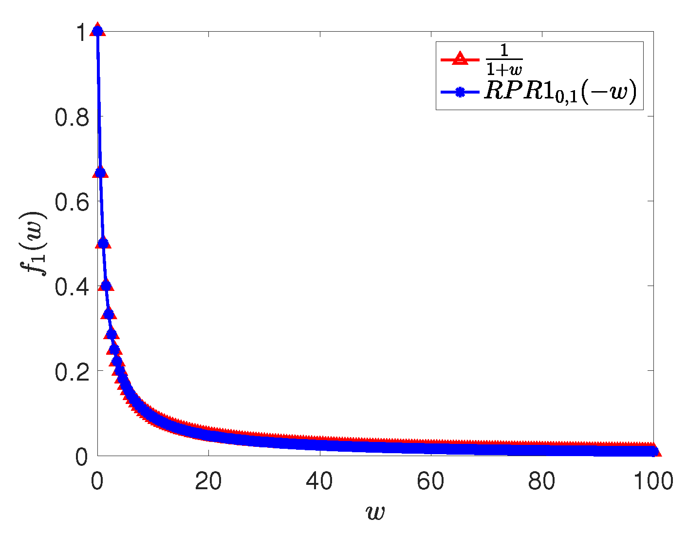
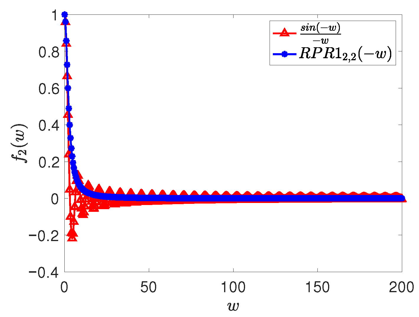
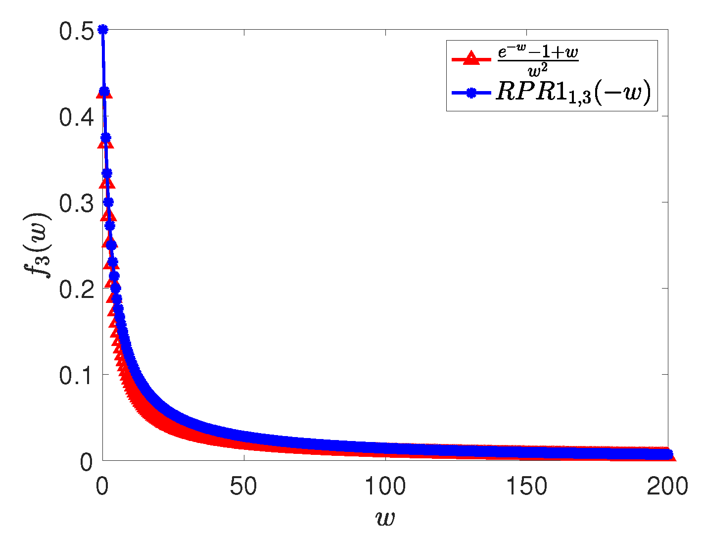
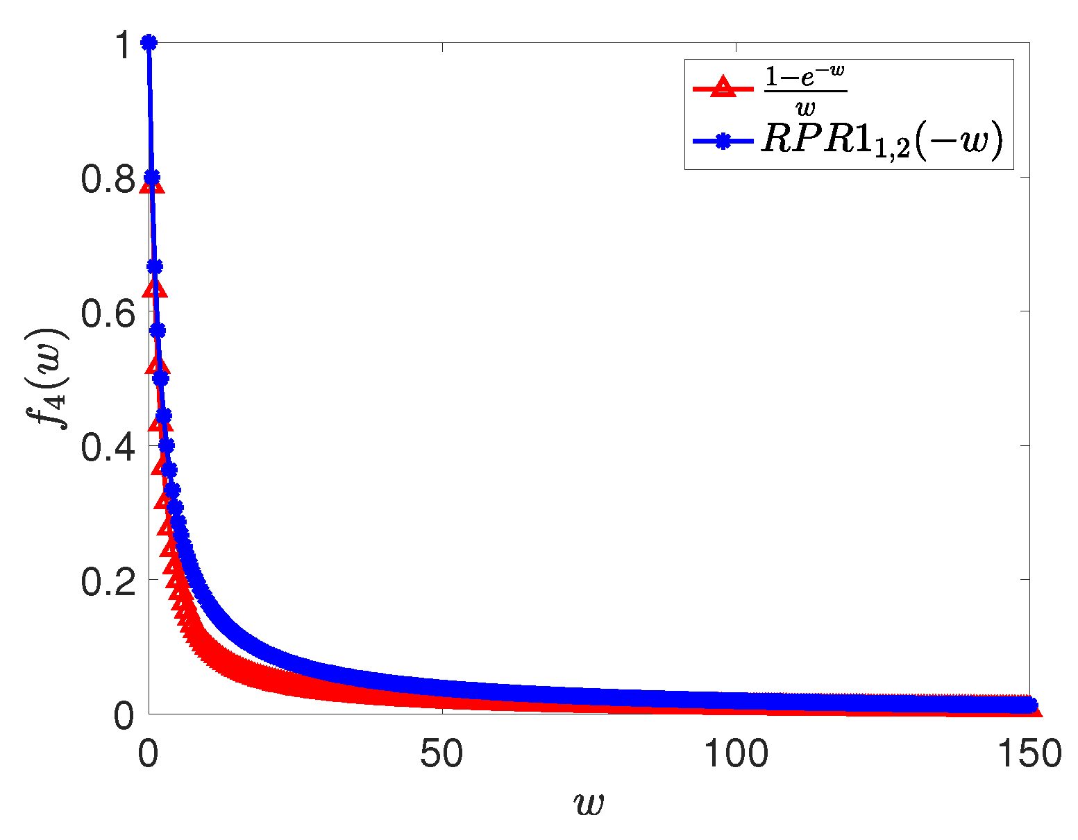
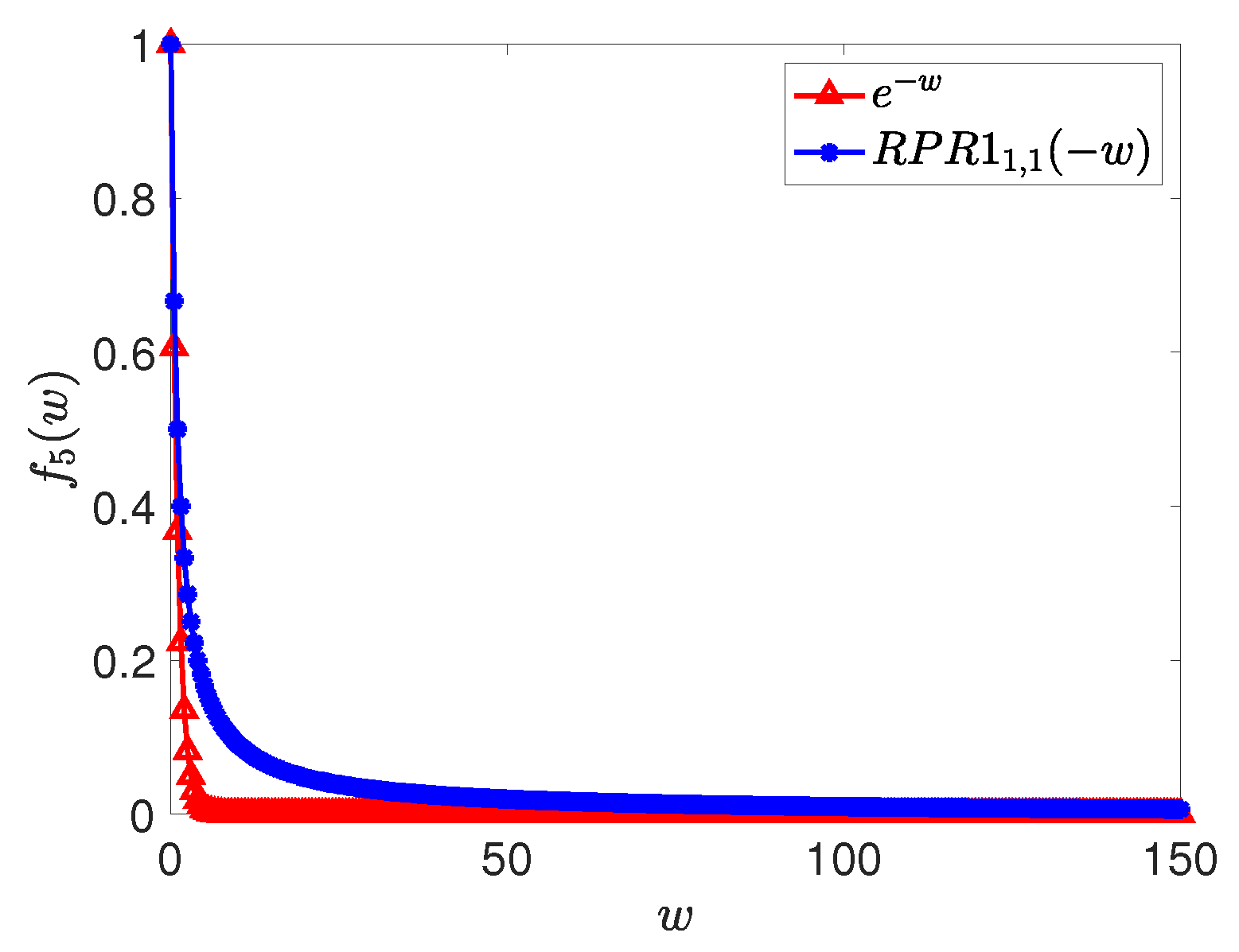
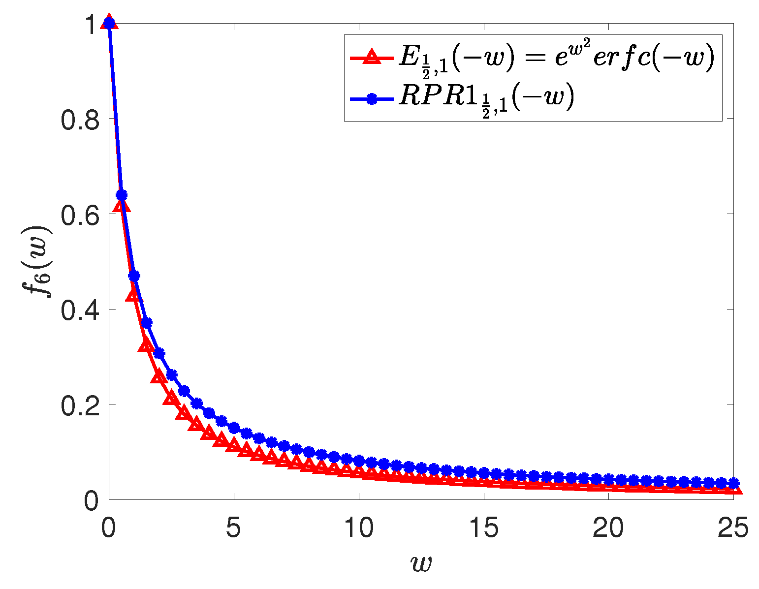
Here, we present some of the special functions discussed in Lemma 2 approximated by the RPR1 approximation in Equation (9) for the MLF. We define the exact special functions in consideration below. The performance of the established RPR1 approximation is compared with the following exact functions, and the results are reported in Figure 1, Figure 2, Figure 3, Figure 4, Figure 5 and Figure 6.

$${\displaystyle f_1\left(w\right)=\frac{1}{1+w},f_2\left(w\right)=\frac{\sin (-w)}{-w},f_3\left(w\right)=\frac{e^{-w}-1+w}{w^2},}$$

$${\displaystyle f_4\left(w\right)=\frac{1-e^{-w}}{w},f_5\left(w\right)=e^{-w},f_6\left(w\right)=e^{w^2}erfc(-w).}$$

Remark 1.

According to the conditions outlined in Theorem 2, we have demonstrated that the proposed approximation RPR1 is L-acceptable. This approximation employs a non-Padé rational approach, effectively reducing unwanted oscillations that can occur due to non-smooth or mismatched initial and boundary conditions in fractional models. The approximation derived in Theorem 1 is based on a local series expansion around $w=0$, and therefore provides first-order accuracy in a neighborhood of the origin. However, it is important to examine the behavior of the approximation for large values of $\left|w\right|.$ For the proposed rational approximation in Equation (9), it can be observed that, as $\left|w\right|$ becomes large, the approximation behaves like

$$R^{+}\left(w\right)\approx {\displaystyle \frac{C}{w}},$$

where C is a constant depending on σ and γ. This indicates that the approximation decays algebraically as $\left|w\right|\to \infty$.

In comparison, the Mittag-Leffler function exhibits different asymptotic behavior depending on the argument. In particular, for large negative arguments, it also decays algebraically, whereas, for large positive arguments, it grows rapidly. Therefore, the proposed approximation does not capture the full asymptotic behavior of the Mittag-Leffler function for all regions of the complex plane. However, in the context of the present work, the argument w arises as $w=-t^{\sigma }G$, where G is a positive definite matrix. Consequently, the spectrum of w lies in the negative real axis, where both the Mittag-Leffler function and the proposed approximation exhibit consistent decay behavior. This ensures that the approximation remains suitable for the intended numerical scheme.

4. Generalized Exponential Time Differencing Schemes

The time-fractional reaction–diffusion equation in n-dimensional space is a generalization of the classical reaction–diffusion equation incorporating a fractional derivative in time to model anomalous diffusion. It is given by

$$\left\{\begin{array}{c}{}^{c}D^{\sigma }w=\kappa \mathrm{\Delta }w+H(w,t),x\in \mathrm{\Omega }\subset {\mathbb{R}}^n,t>0,\hfill \\ w(x,0)=w_0\left(x\right),x\in \mathrm{\Omega },\hfill \\ w(x,t)=g(x,t),x\in \partial \mathrm{\Omega },t>0,\hfill \end{array}\right.$$

(12)

where ${}^{c}D^{\sigma }$ is the Caputo time-fractional derivative operator of order $0<\sigma \le 1$ defined as

$${}^{c}D^{\sigma }w\left(t\right)={\int }_0^t{\displaystyle \frac{{(t-s)}^{-\sigma }}{\mathrm{\Gamma }(1-\sigma )}}{w}^{\prime }\left(s\right)ds,$$

where $\mathrm{\Gamma }(.)$ is the Gamma function. The diffusion coefficient is denoted by $\kappa$. $\mathrm{\Delta }w$ is the Laplacian operator in n-dimensional space given by

$$\mathrm{\Delta }w={\displaystyle \sum _{j=1}^n}{\displaystyle \frac{{\partial }^{2}w}{\partial x_j^2}},$$

with $H(w,t)$ referring to some reasonable nonlinear function of w which is chosen as reaction kinetics. For instance, the one-dimensional fractional nonlinear reaction–diffusion equation is of the form

$${}^{c}D^{\sigma }w=\kappa {\displaystyle \frac{{\partial }^{2}w}{\partial x_1^2}}+H(w,t).$$

(13)

Introducing a uniform mesh of grid points in each spatial direction, the Laplacian operator can be discretized, and it leads the PDE in Equation (12) back to a system of fractional differential equations (DEs), thus allowing us to focus on just a system of DEs. For instance, we look at the derivation of the system of fractional DEs in a 1D case, introducing the uniform spatial discritization as

$$x_i=a+ih,i=0,1,2,\dots ,M\mathrm{with}h={\displaystyle \frac{b-a}{M}}.$$

Using the second-order central difference formula for the spatial discretization,

$${\displaystyle \frac{{\partial }^{2}w}{\partial x^2}}{|}_{x=x_i}\approx {\displaystyle \frac{w_{i+1}\left(t\right)-2w_i\left(t\right)+w_{i-1}\left(t\right)}{h^2}},$$

(14)

where h is the uniform grid spacing and $w_i\left(t\right)\approx w(x_i,t)$. Substituting Equation (14) into Equation (13) for all interior nodes $i=1,2,\dots ,(M-1),$ we get the following system of DEs:

$$\begin{array}{c}{}^{c}D^{\sigma }{w}_1(t)={\displaystyle \frac{\kappa }{h^2}}\left(w_2(t)-2w_1\left(t\right)+w_0\left(t\right)\right)+H(w_1,t)\hfill \\ {}^{c}D^{\sigma }{w}_2(t)={\displaystyle \frac{\kappa }{h^2}}\left(w_3\left(t\right)-2w_2\left(t\right)+w_1\left(t\right)\right)+H(w_2,t)\hfill \\ ⋮\hfill \\ {}^{c}D^{\sigma }{w}_{M-1}\left(t\right)={\displaystyle \frac{\kappa }{h^2}}\left(w_M\left(t\right)-2w_{M-1}\left(t\right)+w_{M-2}\left(t\right)\right)+H(w_{M-1},t),\hfill \end{array}$$

(15)

where the boundary values are given by

$$\begin{array}{c}\hfill w_0\left(t\right)=g(a,t)\mathrm{and}{w}_M\left(t\right)=g(b,t).\end{array}$$

The above system of fractional DEs can be represented by the following semi-discrete system:

$$\left\{\begin{array}{c}{}^{c}D^{\sigma }W\left(t\right)+GW\left(t\right)=\mathcal{H}(W,t),t>0\hfill \\ W\left(t_0\right)=W_0,\hfill \end{array}\right.$$

(16)

where

$$W\left(t\right)=\left[\begin{array}{c}{w}_1\left(t\right)\\ w_2\left(t\right)\\ ⋮\\ w_{M-1}\left(t\right)\end{array}\right],G={\displaystyle \frac{\kappa }{h^2}}\left[\begin{array}{cccccc}2& -1& 0& 0& \dots & 0\\ -1& 2& -1& 0& \dots & 0\\ 0& -1& 2& -1& \dots & 0\\ 0& 0& -1& 2& \dots & 0\\ ⋮& ⋮& ⋮& ⋮& \ddots & -1\\ 0& 0& 0& 0& -1& 2\end{array}\right],$$

and

$$\mathcal{H}(W,t)=\left[\begin{array}{c}H(w_1,t)\\ H(w_2,t)\\ ⋮\\ H(w_{M-1},t)\end{array}\right]+\left[\begin{array}{c}{\displaystyle \frac{\kappa }{h^2}}g(a,t)\\ 0\\ ⋮\\ {\displaystyle \frac{\kappa }{h^2}}g(b,t)\end{array}\right],$$

(17)

where the boundary conditions do not appear in matrix G and are absorbed as extra forcing terms in $\mathcal{H}(W,t).$

The Dirichlet boundary conditions of problem (16) lead the matrix G to be symmetric positive definite, and Lemma 8 can be generalized to the matrix $G.$ Also, the total number of unknowns in the system is equal to the number of grid points in the spatial domain. We assume that the the nonlinear source term $\mathcal{H}:\mathcal{D}\times [0,T]\to \mathbb{R}$ is Lipschitz with respect to the first variable for a suitable region $\mathcal{D}.$ That is,

$$|\mathcal{H}(V_1\left(t\right),t)-\mathcal{H}(V_2\left(t\right),t)|\le L|V_1\left(t\right)-V_2\left(t\right)|,$$

for some $L>0,$ for all $V_1,V_2\in \mathcal{D}.$

Generalized exponential time differencing (GETD) is an extension of the standard exponential time differencing (ETD) method to problems of fractional-order derivatives using the Mittag-Leffler function. In this section, we develop the first-order explicit generalized exponential time differencing scheme for solving time-fractional differential equations of the type given in Equation (16).

4.1. The Derivation of the GETD Scheme

Define

$$\mathcal{L}\left\{W\left(t\right)\right\}=\widehat{W}\left(s\right),\mathrm{and}\mathcal{L}\left\{\mathcal{H}\left(t\right)\right\}=\widehat{\mathcal{H}}\left(s\right).$$

Applying the Laplace transform to both sides of Equation (16), we obtain

$$\mathcal{L}{\{}^c{D}^{\sigma }W\left(t\right)\}+\mathcal{L}\left\{GW\left(t\right)\right\}=\mathcal{L}\left\{\mathcal{H}\left(t\right)\right\},$$

which implies

$$\widehat{W}\left(s\right)=s^{\sigma -1}{\left(s^{\sigma }I+G\right)}^{-1}{W}_0+{\left(s^{\sigma }I+G\right)}^{-1}\widehat{\mathcal{H}}\left(s\right).$$

(18)

Define

$${\epsilon }_{\sigma ,\gamma }(s,G):=s^{\sigma -\gamma }{\left(s^{\sigma }I+G\right)}^{-1}.$$

Hence, Equation (18) can be written explicitly as

$$\widehat{W}\left(s\right)={ϵ}_{\sigma ,1}(s,G)W_0+{ϵ}_{\sigma ,\sigma }(s,G)\widehat{\mathcal{H}}\left(s\right).$$

(19)

By denoting ${\mathrm{\Psi }}_{\sigma ,\gamma }(s,G)$, the inverse Laplace transform of ${\epsilon }_{\sigma ,\gamma }(s,G)$ [52], and by using Lemma 3, we have

$${\mathcal{L}}^{-1}\left\{{\epsilon }_{\sigma ,\gamma }(s,G)\right\}={\mathrm{\Psi }}_{\sigma ,\gamma }(t,G)=t^{\gamma -1}{E}_{\sigma ,\gamma }(-t^{\sigma }G),$$

where $E_{\sigma ,\gamma }$ is the two-parameter Mittag-Leffler function (MLF) as defined in Equation (2).

Taking the Laplace inverse of Equation (19) in both sides,

$$W\left(t\right)={\mathcal{L}}^{-1}\left\{{\epsilon }_{\sigma ,1}(s,G)W_0\right\}+{\mathcal{L}}^{-1}\left\{{\left(s^{\sigma }I+G\right)}^{-1}\widehat{\mathcal{H}}\left(s\right)\right\}.$$

The first Laplace inverse leads to

$${\mathcal{L}}^{-1}\left\{{\epsilon }_{\sigma ,1}(s,G)W_0\right\}=E_{\sigma ,1}(-t^{\sigma }G)W_0.$$

The second Laplace inverse is evaluated by using the convolution integral as follows:

$$\begin{array}{ccc}\hfill {\mathcal{L}}^{-1}\left\{{\left(s^{\sigma }I+G\right)}^{-1}\widehat{\mathcal{H}}\left(s\right)\right\}& =& {\mathcal{L}}^{-1}\left\{{\left(s^{\sigma }I+G\right)}^{-1}\right\}⊛{\mathcal{L}}^{-1}\left\{\widehat{\mathcal{H}}\left(s\right)\right\}\hfill \\ & =& t^{\sigma -1}{E}_{\sigma ,\sigma }(-t^{\sigma }G)⊛\mathcal{H}\left(W\left(t\right)\right)\hfill \\ & =& {\int }_0^t{(t-\eta )}^{\sigma -1}{E}_{\sigma ,\sigma }(-{(t-\eta )}^{\sigma }G)\mathcal{H}\left(W\left(\eta \right)\right)d\eta .\hfill \end{array}$$

Hence, Equation (16) is equivalent to the following integral form:

$$W\left(t\right)=E_{\sigma ,1}(-t^{\sigma }G)W_0+{\int }_0^t{(t-\eta )}^{\sigma -1}{E}_{\sigma ,\sigma }(-{(t-\eta )}^{\sigma }G)\mathcal{H}\left(W\left(\eta \right)\right)d\eta .$$

(20)

4.2. Derivation of Fractional Exponential Time Differencing Scheme (FETD1)

To approximate the solution of Equation (20) in some interval $[0,T]$, we introduce the mesh points

$$0=t_0<t_1<t_2<\dots ,t_N=T.$$

Let $t_{n+\frac{1}{2}}={\displaystyle \frac{t_n+t_{n+1}}{2}},I_n=[t_n,t_{n+1}],k_n=t_{n+1}-t_n$ for $n=0,1,2,\dots ,N-1.$ Let k denote the maximum size of the mesh element.

The resulting method of replacing $\mathcal{H}\left(W\right(\eta \left)\right)$ in each subinterval $[t_i,t_{i+1}]$ with a suitable interpolating polynomial and then evaluating the integrals is named fractional exponential time differencing (FETD). In this paper, we use the constant interpolating polynomial of degree 0,

$$\begin{array}{ccc}\hfill {\mathcal{P}}_i^0[\mathcal{H}:\eta ]& =& {\mathcal{H}}^i,\hfill \end{array}$$

to approximate $\mathcal{H}\left(W\right(\eta \left)\right)$ on each subinterval $I_i$.

By setting $W_n\approx W\left(t_n\right)$, the variation of the constant formula in Equation (20) can be written in a piecewise form:

$$\begin{array}{ccc}\hfill W_n& =& E_{\sigma ,1}(-t_n^{\sigma }G)W^0+{\int }_0^{t_1}{(t_n-\eta )}^{\sigma -1}{E}_{\sigma ,\sigma }(-G{(t_n-\eta )}^{\sigma }){\mathcal{P}}_0^0[\mathcal{H}:\eta ]d\eta \hfill \\ & & +{\int }_{t_1}^{t_2}{(t_n-\eta )}^{\sigma -1}{E}_{\sigma ,\sigma }(-G{(t_n-\eta )}^{\sigma }){\mathcal{P}}_1^0[\mathcal{H}:\eta ]d\eta \hfill \\ & & +{\int }_{t_2}^{t_3}{(t_n-\eta )}^{\sigma -1}{E}_{\sigma ,\sigma }(-G{(t_n-\eta )}^{\sigma }){\mathcal{P}}_2^0[\mathcal{H}:\eta ]d\eta \hfill \\ & & +\dots +{\int }_{t_{n-1}}^{t_n}{(t_n-\eta )}^{\sigma -1}{E}_{\sigma ,\sigma }(-G{(t_n-\eta )}^{\sigma }){\mathcal{P}}_{n-1}^0[\mathcal{H}:\eta ]d\eta .\hfill \end{array}$$

Hence, we obtain

$$W_n=E_{\sigma ,1}(-t_n^{\sigma }G)W^0+{\displaystyle \sum _{i=0}^{n-1}}{\int }_{t_i}^{t_{i+1}}{(t_n-\eta )}^{\sigma -1}{E}_{\sigma ,\sigma }(-{(t_n-\eta )}^{\sigma }G){\mathcal{P}}_i^0[\mathcal{H}:\eta ]d\eta .$$

(21)

Substituting the interpolating polynomial of degree 0 (${\mathcal{P}}_i^0[\mathcal{H}:\eta ]={\mathcal{H}}^i$) into the FETD scheme in (21) will generate the first-order FETD scheme (FETD1). We now focus on the derivation of the FETD1 scheme. Substituting ${\mathcal{H}}^i$ in Equation (21), we have

$$W_n=E_{\sigma }(-t_n^{\sigma }G)W^0+{\displaystyle \sum _{i=0}^{n-1}}{\int }_{t_i}^{t_{i+1}}{(t_n-\eta )}^{\sigma -1}{E}_{\sigma ,\sigma }(-{(t_n-\eta )}^{\sigma }G){\mathcal{H}}^{i}d\eta .$$

(22)

Lemma 9.

Let $0<\sigma \le 1$. Then,

$$\begin{array}{c}{\displaystyle \sum _{i=0}^{n-1}}{\int }_{t_i}^{t_{i+1}}{(t_n-\eta )}^{\sigma -1}{E}_{\sigma ,\sigma }(-{(t_n-\eta )}^{\sigma }G){\mathcal{H}}^{i}d\eta ={\displaystyle \sum _{i=1}^{n-1}}{(t_n-t_i)}^{\sigma }{E}_{\sigma ,\sigma +1}(-{(t_n-t_i)}^{\sigma }G)\hfill \\ ({\mathcal{H}}^i-{\mathcal{H}}^{i-1})+t_n^{\sigma }{E}_{\sigma ,\sigma +1}(-t_n^{\sigma }G){\mathcal{H}}^0.\hfill \end{array}$$

(23)

Proof. 

Define

$$I={\displaystyle \sum _{i=0}^{n-1}}{\int }_{t_i}^{t_{i+1}}{(t_n-\eta )}^{\sigma -1}{E}_{\sigma ,\sigma }(-{(t_n-\eta )}^{\sigma }G){\mathcal{H}}^{i}d\eta .$$

Using Lemma 5 and Equation (4),

$$\begin{array}{c}I={\displaystyle \sum _{i=0}^{n-1}}{\int }_{t_i}^{t_{i+1}}{(t_n-\eta )}^{\sigma -1}{E}_{\sigma ,\sigma }(-{(t_n-\eta )}^{\sigma }G)d\eta {\mathcal{H}}^i\hfill \\ \hfill \\ ={\displaystyle \sum _{i=0}^{n-1}}{\int }_{t_i}^{t_{i+1}}{e}_{\sigma ,\sigma }(t_n-\eta ;G)d\eta {\mathcal{H}}^i\hfill \\ \hfill \\ ={\displaystyle \sum _{i=0}^{n-1}}\left(e_{\sigma ,\sigma +1}(t_n-t_i;G)-e_{\sigma ,\sigma +1}(t_n-t_{i+1};G)\right)d\eta {\mathcal{H}}^i\hfill \\ \hfill \\ ={\displaystyle \sum _{i=0}^{n-1}}({(t_n-t_i)}^{\sigma }{E}_{\sigma ,\sigma +1}(-{(t_n-t_i)}^{\sigma }G)-{(t_n-t_{i+1})}^{\sigma }{E}_{\sigma ,\sigma +1}(-{(t_n-t_{i+1})}^{\sigma }G)){\mathcal{H}}^i\hfill \\ \hfill \\ =t_n^{\sigma }{E}_{\sigma ,\sigma +1}(-t_n^{\sigma }G){\mathcal{H}}^0+\left[{(t_n-t_1)}^{\sigma }{E}_{\sigma ,\sigma +1}(-{(t_n-t_1)}^{\sigma }G)({\mathcal{H}}^1-{\mathcal{H}}^0)\right]\hfill \\ \hfill \\ +\left[{(t_n-t_2)}^{\sigma }{E}_{\sigma ,\sigma +1}(-{(t_n-t_2)}^{\sigma }G)({\mathcal{H}}^2-{\mathcal{H}}^1)\right]\hfill \\ \hfill \\ +\left[{(t_n-t_3)}^{\sigma }{E}_{\sigma ,\sigma +1}(-{(t_n-t_3)}^{\sigma }G)({\mathcal{H}}^3-{\mathcal{H}}^2)\right]\hfill \\ \hfill \\ +\dots +\left[{(t_n-t_{n-1})}^{\sigma }{E}_{\sigma ,\sigma +1}(-{(t_n-t_{n-1})}^{\sigma }G)({\mathcal{H}}^{n-1}-{\mathcal{H}}^{n-2})\right]\hfill \\ \hfill \\ =t_n^{\sigma }{E}_{\sigma ,\sigma +1}(-t_n^{\sigma }G){\mathcal{H}}^0+{\displaystyle \sum _{i=1}^{n-1}}{(t_n-t_i)}^{\sigma }{E}_{\sigma ,\sigma +1}(-{(t_n-t_i)}^{\sigma }G)({\mathcal{H}}^i-{\mathcal{H}}^{i-1}).\hfill \end{array}$$

(24)

Hence, the result follows.    □

Using Lemma 9 in Equation (22), we obtain the FETD1 scheme as follows:

$$\begin{array}{c}{W}_n=E_{\sigma }(-t_n^{\sigma }G)W^0+t_n^{\sigma }{E}_{\sigma ,\sigma +1}(-t_n^{\sigma }G){\mathcal{H}}^0\hfill \\ \hfill \\ +{\displaystyle \sum _{i=1}^{n-1}}{(t_n-t_i)}^{\sigma }{E}_{\sigma ,\sigma +1}(-{(t_n-t_i)}^{\sigma }G)({\mathcal{H}}^i-{\mathcal{H}}^{i-1}).\hfill \end{array}$$

(25)

Theorem 3.

Let G be an invertible matrix, $m_1={\displaystyle \frac{1}{\mathrm{\Gamma }(\sigma +1)}}$ and $m_2={\displaystyle \frac{\mathrm{\Gamma }(\sigma +1)}{\mathrm{\Gamma }(2\sigma +1)}}$. Define $t_{ni}=t_n-t_i.$ Then, the scheme given in Equation (25) is equivalent to

$$\begin{array}{c}{W}_n={(I+m_1{t}_n^{\sigma }G)}^{-1}{W}^0+m_1{t}_n^{\sigma }{\left(I+m_2{t}_n^{\sigma }G\right)}^{-1}{\mathcal{H}}^0\hfill \\ \hfill \\ +{\displaystyle \sum _{i=1}^{n-1}}{t}_{ni}^{\sigma }{m}_1{\left(I+m_2{t}_{ni}^{\sigma }G\right)}^{-1}({\mathcal{H}}^i-{\mathcal{H}}^{i-1}).\hfill \end{array}$$

(26)

Proof. 

We consider the FETD1 scheme in Equation (25) with the RPR1 approximation in Equation (9) to evaluate the terms in the scheme. The first term in the scheme reduces as follows:

$$\begin{array}{cc}{E}_{\sigma }(-t_n^{\sigma }G)W^0\hfill & ={(I+a_2^{*}{t}_n^{\sigma }G)}^{-1}{W}^0\hfill \\ & =(I+{\displaystyle \frac{1}{\mathrm{\Gamma }(\alpha +1)}}{t}_n^{\sigma }G{)}^{-1}{W}^0\hfill \\ & ={(I+m_1{t}_n^{\sigma }G)}^{-1}{W}^0.\hfill \end{array}$$

(27)

Considering the second term in the scheme (25),

$$\begin{array}{cc}{t}_n^{\sigma }{E}_{\sigma ,\sigma +1}(-t_n^{\sigma }G){\mathcal{H}}^0\hfill & =t_n^{\sigma }{\displaystyle \frac{1}{\mathrm{\Gamma }(\sigma +1)}}{(I+a_2^{*}{t}_n^{\sigma }G)}^{-1}{\mathcal{H}}^0\hfill \\ & =m_1{t}_n^{\sigma }{\left(I+{\displaystyle \frac{\mathrm{\Gamma }(\sigma +1)}{\mathrm{\Gamma }(2\sigma +1)}}{t}_n^{\sigma }G\right)}^{-1}{\mathcal{H}}^0\hfill \\ & =m_1{t}_n^{\sigma }{\left(I+m_2{t}_n^{\sigma }G\right)}^{-1}{\mathcal{H}}^0.\hfill \end{array}$$

(28)

The last term in the scheme (25) can be simplified as follows:

$$\begin{array}{ccc}\hfill {\displaystyle \sum _{i=1}^{n-1}}{t}_{ni}^{\sigma }{E}_{\sigma ,\sigma +1}(-t_{ni}^{\sigma }G)({\mathcal{H}}^i-{\mathcal{H}}^{i-1})& =& {\displaystyle \sum _{i=1}^{n-1}}{t}_{ni}^{\sigma }{\displaystyle \frac{1}{\mathrm{\Gamma }(\sigma +1)}}{(I+a_2^{*}{t}_{ni}^{\sigma }G)}^{-1}({\mathcal{H}}^i-{\mathcal{H}}^{i-1})\hfill \\ & =& {\displaystyle \sum _{i=1}^{n-1}}{t}_{ni}^{\sigma }{m}_1{\left(I+{\displaystyle \frac{\mathrm{\Gamma }(\sigma +1)}{\mathrm{\Gamma }(2\sigma +1)}}{t}_{ni}^{\sigma }G\right)}^{-1}({\mathcal{H}}^i-{\mathcal{H}}^{i-1})\hfill \\ & =& {\displaystyle \sum _{i=1}^{n-1}}{t}_{ni}^{\sigma }{m}_1{\left(I+m_2{t}_{ni}^{\sigma }G\right)}^{-1}({\mathcal{H}}^i-{\mathcal{H}}^{i-1}).\hfill \end{array}$$

Finally, by using Equations (27)–(29), the equivalent scheme can be written as

$$\begin{array}{c}{W}_n={(I+m_1{t}_n^{\sigma }G)}^{-1}{W}^0+m_1{t}_n^{\sigma }{\left(I+m_2{t}_n^{\sigma }G\right)}^{-1}{\mathcal{H}}^0\hfill \\ \hfill \\ +{\displaystyle \sum _{i=1}^{n-1}}{t}_{ni}^{\sigma }{m}_1{\left(I+m_2{t}_{ni}^{\sigma }G\right)}^{-1}({\mathcal{H}}^i-{\mathcal{H}}^{i-1}).\hfill \end{array}$$

(29)

  □

We call the scheme in Equation (29) the fractional exponential time differencing with real pole rational approximation (FETD-RPR1) scheme. The parallel implementation of the FETD-RPR1 scheme is given below.

Remark 2.

The efficient implementation $a_n,b_n,c_n$, which includes computation of matrix inverses, is computed using LU decomposition. Although the computational complexity of LU decomposition is similar to direct computation of inverses (O($n^3$)), this is much faster and numerically more stable than computing direct inverses.

5. Convergence Analysis

We first prove the following Lemma (Grönwall-type inequality), which our main convergence theorem relies on.

Lemma 10.

Let $w_n$ be a sequence of non-negative real numbers such that

$$w_n\le M{(t_n-t_0)}^{\sigma +s-1}+L{h}^{\sigma }{\displaystyle \sum _{i=0}^{n-1}}{(n-i)}^{\sigma }{E}_{\sigma ,\sigma +1}(-{(n-i)}^{\sigma }Z)w_i,$$

where $0<\sigma <1,0<s<1$ and $n=0,1,2,\dots ,N$ with $M,L$ being positive constants. Then,

$$w_n\le M\mathrm{\Gamma }(\sigma +s){(t_n-t_0)}^{\sigma +s}{E}_{\sigma ,\sigma +s}\left({(t_n-t_0)}^{\sigma +1}{\displaystyle \frac{L}{\sigma }}\right).$$

Proof. 

By simply applying Lemma 8, we have

$$w_n\le M{(t_n-t_0)}^{\sigma +s-1}+{\displaystyle \frac{L{h}^{\sigma }}{\mathrm{\Gamma }(\sigma +1)}}{\displaystyle \sum _{i=0}^{n-1}}{(n-i)}^{\sigma }{w}_i.$$

We refer to the proof of Corollary 2.1 in [53] with $y_n=M{(t_n-t_0)}^{\sigma +s-1}$ with the sequence ${\left\{y_{n,j}\right\}}_{j=0}^{\infty }$ in the following manner:

$$y_{n,1}=y_n{y}_{n,j}={\displaystyle \frac{L{h}^{\sigma }}{\mathrm{\Gamma }(\sigma +1)}}{\displaystyle \sum _{i=0}^{n-1}}{(n-i)}^{\sigma }{y}_{i,j-1},\mathrm{for}j\ge 2.$$

Then, as in the proof of Corollary 2.1 in [53], we have

$$w_n\le {\displaystyle \sum _{j=1}^{\infty }}{y}_{n,j},n=0,1,2,\dots ,N.$$

(30)

Also, we can use induction to prove that

$$y_{n,j}=\mathrm{\Gamma }(\sigma +s)M{\left({\displaystyle \frac{L}{\sigma }}\right)}^{j-1}{\displaystyle \frac{h^{j(\sigma +1)+s-1}{n}^{j(\sigma +1)+s-1}}{\mathrm{\Gamma }(\sigma j+s)}}.$$

Hence, Equation (30) gives

$$\begin{array}{ccc}\hfill w_n& \le & {\displaystyle \sum _{j=1}^{\infty }}\mathrm{\Gamma }(\sigma +s)M{\left({\displaystyle \frac{L}{\sigma }}\right)}^{j-1}{\displaystyle \frac{h^{j(\sigma +1)+s-1}{n}^{j(\sigma +1)+s-1}}{\mathrm{\Gamma }(\sigma j+s)}}\hfill \\ & =& M\mathrm{\Gamma }(\sigma +s){\displaystyle \sum _{j=1}^{\infty }}{\left({\displaystyle \frac{L}{\sigma }}\right)}^{j-1}{\displaystyle \frac{{(t_n-t_0)}^{j(\sigma +1)+s-1}}{\mathrm{\Gamma }(\sigma j+s)}}\hfill \\ & =& M\mathrm{\Gamma }(\sigma +s){\displaystyle \sum _{j=0}^{\infty }}{\left({\displaystyle \frac{L}{\sigma }}\right)}^j{\displaystyle \frac{{(t_n-t_0)}^{(j+1)(\sigma +1)+s-1}}{\mathrm{\Gamma }\left(\sigma \right(j+1)+s)}}\hfill \\ & =& M\mathrm{\Gamma }(\sigma +s){(t_n-t_0)}^{\sigma +s}{\displaystyle \sum _{j=0}^{\infty }}{\left({\displaystyle \frac{L}{\sigma }}\right)}^j{\displaystyle \frac{{(t_n-t_0)}^{(\sigma +1)j}}{\mathrm{\Gamma }(\sigma j+\sigma +s)}}.\hfill \end{array}$$

Hence, we have

$$w_n\le M\mathrm{\Gamma }(\sigma +s){(t_n-t_0)}^{\sigma +s}{E}_{\sigma ,\sigma +s}\left({(t_n-t_0)}^{\sigma +1}{\displaystyle \frac{L}{\sigma }}\right).$$

(31)

  □

Theorem 4.

Suppose that $0<\sigma <1.$ Then, the numerical solution given in Equation (25) satisfies

$$|W\left(t_n\right)-W_n|\le Dh,n=1,2,\dots ,N,$$

where D does not depend on h and $N=⌊{\displaystyle \frac{T}{h}}⌋.$

Proof. 

Assuming ${\mathcal{H}}^{-1}=0$, the error of the GETD1 method can be written as

$$\begin{array}{ccc}\hfill W\left(t_n\right)-W_n& =& {\int }_{t_0}^{t_n}{(t-\eta )}^{\sigma -1}{E}_{\sigma ,\sigma }(-{(t-\eta )}^{\sigma }G)\mathcal{H}\left(W\left(\eta \right)\right)d\eta -t_n^{\sigma }{E}_{\sigma ,\sigma +1}(-{\left(t_n\right)}^{\sigma }G){\mathcal{H}}^0\hfill \\ & & -{\displaystyle \sum _{i=1}^{n-1}}{(t_n-t_i)}^{\sigma }{E}_{\sigma ,\sigma +1}(-{(t_n-t_i)}^{\sigma }G)({\mathcal{H}}^i-{\mathcal{H}}^{i-1})\hfill \\ & =& {\int }_{t_0}^{t_n}{(t-\eta )}^{\sigma -1}{E}_{\sigma ,\sigma }(-{(t-\eta )}^{\sigma }G)\mathcal{H}\left(W\left(\eta \right)\right)d\eta \hfill \\ & & -{\displaystyle \sum _{i=0}^{n-1}}{(t_n-t_i)}^{\sigma }{E}_{\sigma ,\sigma +1}(-{(t_n-t_i)}^{\sigma }G)({\mathcal{H}}^i-{\mathcal{H}}^{i-1}).\hfill \end{array}$$

Hence, the error of the FETD1 method can be represented as

$$\begin{array}{c}W\left(t_n\right)-W_n={\int }_{t_0}^{t_n}{(t-\eta )}^{\sigma -1}{E}_{\sigma ,\sigma }(-{(t-\eta )}^{\sigma }G)\mathcal{H}\left(W\left(\eta \right)\right)d\eta \hfill \\ \hfill \\ -{\displaystyle \sum _{i=0}^{n-1}}{(t_n-t_i)}^{\sigma }{E}_{\sigma ,\sigma +1}(-{(t_n-t_i)}^{\sigma }G)(\mathcal{H}\left(W\left(t_i\right)\right)-\mathcal{H}\left(W\left(t_{i-1}\right)\right))\hfill \\ \hfill \\ +{\displaystyle \sum _{i=0}^{n-1}}{(t_n-t_i)}^{\sigma }{E}_{\sigma ,\sigma +1}(-{(t_n-t_i)}^{\sigma }G)(\mathcal{H}\left(W\left(t_i\right)\right)-\mathcal{H}\left(W\left(t_{i-1}\right)\right))\hfill \\ \hfill \\ -{\displaystyle \sum _{i=0}^{n-1}}{(t_n-t_i)}^{\sigma }{E}_{\sigma ,\sigma +1}(-{(t_n-t_i)}^{\sigma }G)(\mathcal{H}\left(W_i\right)-\mathcal{H}\left(W_{i-1}\right))\hfill \\ \hfill \\ =\zeta \left[\mathcal{H}\right(W\left(t\right)\left)\right]\hfill \\ \hfill \\ +{\displaystyle \sum _{i=0}^{n-1}}{(t_n-t_i)}^{\sigma }{E}_{\sigma ,\sigma +1}(-{(t_n-t_i)}^{\sigma }G)\hfill \\ \hfill \\ \left([\mathcal{H}\left(W\left(t_i\right)\right)-\mathcal{H}\left(W_i\right)]-[\mathcal{H}\left(W\left(t_{i-1}\right)\right)-\mathcal{H}\left(W_{i-1}\right)])\right),\hfill \end{array}$$

(32)

where

$$\begin{array}{ccc}\hfill \zeta \left[f\right]& =& {\displaystyle {\int }_{t_0}^{t_n}{(t-\eta )}^{\sigma -1}{E}_{\sigma ,\sigma }(-{(t-\eta )}^{\sigma }G)f\left(\eta \right)d\eta }\hfill \\ & & -{\displaystyle \sum _{i=0}^{n-1}}{(t_n-t_i)}^{\sigma }{E}_{\sigma ,\sigma +1}(-{(t_n-t_i)}^{\sigma }G)(\mathcal{H}\left(W\left(t_i\right)\right)-\mathcal{H}\left(W\left(t_{i-1}\right)\right)).\hfill \end{array}$$

By the Lipschitz continuity of $\mathcal{H}$,

$$\begin{array}{ccc}\hfill |W\left(t_n\right)-W_n|& =& \left|E\right(\mathcal{H}oW\left)\right|\hfill \\ & & +L{\displaystyle \sum _{i=0}^{n-1}}{(t_n-t_i)}^{\sigma }{E}_{\sigma ,\sigma +1}(-{(t_n-t_i)}^{\sigma }G)\hfill \\ & & \left(|W\left(t_i\right)-W_i|+|W\left(t_{i-1}\right)-W_{i-1}|\right).\hfill \end{array}$$

Assuming $\mathcal{H}$ to be sufficiently smooth, it is a well-known result that $W\left(t\right)$ has an expansion in mixed powers of $(t-t_0)$ and ${(t-t_0)}^{\sigma }$. Hence, for our analysis, we assume it is reasonable to assume that the smoothness of $\mathcal{H}$ brings about a similar behavior for the composite function $\mathcal{H}\left(W\right(t\left)\right)$ too. Therefore, we assume the following assumption for our further analysis: the function $\mathcal{H}\in C^2\left(D\right)$ and $\mathcal{H}\left(W\left(t\right)\right)={\sum }_{l=1}^L{d}_j{(t-t_0)}^{l\sigma }+o(t-t_0)$ for some $d_j\in \mathbb{R}$ and L is the greatest integer such that $\sigma L<1.$ Now, we focus on $E\left[g\right]$ where $g\left(t\right)={(t-t_0)}^k$ for $0<k<1$.

Assume that g is sufficiently smooth in $[s,t_n]$ for a given $s>t_0$ and let m be the smallest integer such that $s\le t_m.$ We now study the behavior of g by splitting the interval of integration $[t_0,t_n]$ into $[t_0,t_m]$ and $[t_m,t_n]$ with ${\zeta }_1\left[g\right]$ and ${\zeta }_2\left[g\right]$ as the error from $[t_0,t_m]$ and $[t_m,t_n]$, respectively. First, we focus on ${\zeta }_1\left[g\right]$ where the function g has a lack of smoothness:

$$\begin{array}{ccc}\hfill {\zeta }_1\left[g\right]& =& {\displaystyle \sum _{i=0}^{m-1}}{\int }_{t_i}^{t_{i+1}}{(t_n-\eta )}^{\sigma -1}{E}_{\sigma ,\sigma }(-{(t_n-\eta )}^{\sigma }G)g\left(\eta \right)d\eta \hfill \\ & & -{\displaystyle \sum _{i=0}^{m-1}}{(t_n-t_i)}^{\sigma }{E}_{\sigma ,\sigma +1}(-{(t_n-t_i)}^{\sigma }G)(g\left(t_i\right)-g\left(t_{i-1}\right)).\hfill \end{array}$$

Using Lemma 4 when $r=0$ in the Lemma, we have

$$\begin{array}{c}{\zeta }_1\left[g\right]={\displaystyle \sum _{i=0}^{m-1}}{\int }_{t_i}^{t_{i+1}}{(t_n-\eta )}^{\sigma -1}{E}_{\sigma ,\sigma }(-{(t_n-\eta )}^{\sigma }G)g\left(\eta \right)d\eta \hfill \\ \hfill \\ -{\displaystyle \sum _{i=0}^{m-1}}{\int }_{t_i}^{t_{i+1}}{(t_n-\eta )}^{\sigma -1}{E}_{\sigma ,\sigma }(-{(t_n-\eta )}^{\sigma }G)(g\left(t_i\right)-g\left(t_{i-1}\right))d\eta \hfill \\ \hfill \\ |{\zeta }_1\left[g\right]|={\displaystyle \sum _{i=0}^{m-1}}{\int }_{t_i}^{t_{i+1}}{(t_n-\eta )}^{\sigma -1}{E}_{\sigma ,\sigma }(-{(t_n-\eta )}^{\sigma }G)|g\left(\eta \right)-g\left(t_i\right)+g\left(t_{i-1}\right)|d\eta .\hfill \end{array}$$

(33)

Also, we can prove that

$$\begin{array}{cc}|g\left(\eta \right)-g\left(t_i\right)+g\left(t_{i-1}\right)|\hfill & \le |{(t_{i+1}-t_0)}^k-{(t_i-t_0)}^k+{(t_{i-1}-t_0)}^k|\hfill \\ & =\left|h^k\left({(i+1)}^k-i^k+{(i-1)}^k\right)\right|\le h^k{N}_1,\hfill \end{array}$$

(34)

for some $N_1\in \mathbb{R}.$ Then, by using Lemma 8 in Equation (33) and telescoping the series sum, and, for some $n_0>n$ with $n_0\in \mathbb{R}$, we have

$$\begin{array}{ccc}\hfill |{\zeta }_1\left[g\right]|& \le & {\displaystyle \sum _{i=0}^{m-1}}{\int }_{t_i}^{t_{i+1}}{\displaystyle \frac{{(t_n-\eta )}^{\sigma -1}}{\mathrm{\Gamma }\left(\sigma \right)}}{h}^{k}Nd\eta \hfill \\ & =& {\displaystyle \frac{h^{k}N}{\mathrm{\Gamma }(\sigma +1)}}[{(t_n-t_i)}^{\sigma }-{(t_n-t_{i+1})}^{\sigma }]\hfill \\ & \le & M_1{h}^{k+1}{(t_n-t_0)}^{\sigma -1},\hfill \end{array}$$

where $M_1={\displaystyle \frac{nN}{\mathrm{\Gamma }(\sigma +1)}}$. Now, we examine the error on $[t_m,t_n]$ where the function g can be considered as sufficiently smooth. As in Theorem 4.2 in [30],

$$\begin{array}{ccc}\hfill {\zeta }_2\left[g\right]& =& h{\int }_{t_m}^{t_n}{(t_n-\eta )}^{\sigma -1}{E}_{\sigma ,\sigma }(-{(t_n-\eta )}^{\sigma }G)k{(\eta -t_0)}^{k-1}d\eta \hfill \\ & \le & hk{\int }_{t_m}^{t_n}{(t_n-\eta )}^{\sigma -1}{E}_{\sigma ,\sigma }(-{(t_n-\eta )}^{\sigma }G){(\eta -t_0)}^{k-1}d\eta .\hfill \end{array}$$

By using Lemma 4 (when $r=k-1$) and Lemma 8, we have

$$\begin{array}{ccc}{\zeta }_2\left[g\right]\hfill & \le \hfill & hk\mathrm{\Gamma }\left(k\right){(t_n-t_0)}^{\gamma +k-1}{E}_{\sigma ,k}(-{(t_n-t_0)}^{\sigma }Q)\hfill \\ \hfill & \le \hfill & hk\mathrm{\Gamma }\left(k\right){\displaystyle \frac{{(t_n-t_0)}^{\sigma +k-1}}{\mathrm{\Gamma }(\sigma +k)}}\hfill \\ \hfill & =\hfill & M_{2}h{(t_n-t_0)}^{\sigma +k-1},\hfill \end{array}$$

(35)

where $M_2={\displaystyle \frac{k\mathrm{\Gamma }\left(k\right)}{\mathrm{\Gamma }(\sigma +k)}}$. Hence, we can find $M\in \mathbb{R}$ such that

$$\zeta \left[g\right]={\zeta }_1\left[g\right]+{\zeta }_2\left[g\right]\le Mh{(t_n-t_0)}^{\sigma +k-1}.$$

Since we have studied the error behavior of function g, we now focus on the assumption we made earlier about $\mathcal{H}\left(W\right(t\left)\right).$ Then, Equation (15) becomes

$$\begin{array}{ccc}|V\left(t_n\right)-V_n|\hfill & \le \hfill & Mh{(t_n-t_0)}^{2\sigma -1}\hfill \\ \hfill & \hfill & +L{\displaystyle \sum _{i=0}^{n-1}}(t_n-t_i{)}^{\sigma }{E}_{\sigma ,\sigma +1}(-{(t_n-t_i)}^{\sigma }G)\left(|V\left(t_i\right)-V_i|+|V\left(t_{i-1}\right)-V_{i-1}|\right)\hfill \\ \hfill & =\hfill & Mh{(t_n-t_0)}^{2\sigma -1}\hfill \\ \hfill & \hfill & +L{h}^{\sigma }{\displaystyle \sum _{i=0}^{n-1}}{(n-i)}^{\sigma }{E}_{\sigma ,\sigma +1}(-{(t_n-t_i)}^{\sigma }Q)\left(|V\left(t_i\right)-V_i|+|V\left(t_{i-1}\right)-V_{i-1}|\right)\hfill \\ \hfill & =\hfill & Mh{(t_n-t_0)}^{2\sigma -1}\hfill \\ \hfill & \hfill & +L{h}^{\sigma }{\displaystyle \sum _{i=0}^{n-1}}{(n-i)}^{\sigma }{E}_{\sigma ,\sigma +1}(-{(n-i)}^{\sigma }Z)\left(|V\left(t_i\right)-V_i|+|V\left(t_{i-1}\right)-V_{i-1}|\right),\hfill \end{array}$$

(36)

where $Z=h^{\sigma }Q.$ Finally, by directly applying Lemma 10 to Equation (36), and for any $n_0\ge n$, we have

$$\begin{array}{ccc}\hfill |V\left(t_n\right)-V_n|& \le & M\mathrm{\Gamma }\left(2\sigma \right){(t_n-t_0)}^{2\sigma }{E}_{\sigma ,2\sigma }\left({(t_n-t_0)}^{\sigma +1}{\displaystyle \frac{L}{\sigma }}\right)\hfill \\ & \le & M{n}_{0}h\mathrm{\Gamma }\left(2\sigma \right){(t_n-t_0)}^{2\sigma -1}{E}_{\sigma ,2\sigma }\left({(t_n-t_0)}^{\sigma +1}{\displaystyle \frac{L}{\sigma }}\right)\hfill \\ \hfill |V\left(t_n\right)-V_n|& \le & M^{\prime }h\mathrm{\Gamma }\left(2\sigma \right){(t_n-t_0)}^{2\sigma -1}{E}_{\sigma ,2\sigma }\left({(t_n-t_0)}^{\sigma +1}{\displaystyle \frac{L}{\sigma }}\right).\hfill \end{array}$$

Hence, we can prove that there exists a constant D which does not depend on h such that

$$|V\left(t_n\right)-V_n|\le Dh,n=1,2,\dots ,N,$$

which completes the proof.    □

6. Numerical Experiments

In this section, we present numerical experiments to demonstrate the effectiveness and convergence of the proposed scheme (FETD-RPR1), which employs a first-order approximation for the MLF. We apply the developed algorithm to solve various test problems involving linear, nonlinear, and systems of time-fractional reaction–diffusion equations. An accurate convergence order is observed, along with outstanding performance characterized by reduced computational error and time across all examples. We further examine the error and CPU time for each example with different values of $\sigma =0.2,0.4,0.6,0.8.$ The efficiency of the proposed scheme in solving time-fractional reaction–diffusion models is compared with the L1 scheme [54,55], which is another existing first-order method. This scheme utilizes the L1 discretization of the Caputo fractional derivative with the usual central difference of the Laplacian operator. Also, in each example, each dimension of the spatial domain is discretized with $M+1$ spatial nodes with spatial step size $h={\displaystyle \frac{b-a}{M}}$, where $a,b$ are the boundaries for each spatial domain. All codes are executed in MATLAB R2023b, and the experiments are conducted on a laptop (Apple M2Pro) equipped with a 12-core CPU, 19-core GPU, and 16 GB of RAM.

Example 1.

Consider the following linear time-fractional reaction–diffusion equation:

$$\left\{\begin{array}{c}{}^{c}D^{\sigma }w=\epsilon {\displaystyle \frac{{\partial }^{2}w}{\partial x^2}}+\epsilon w+g(x,t),t\ge 0,x\in \left[-{\displaystyle \frac{\pi }{2}},{\displaystyle \frac{\pi }{2}}\right],\hfill \\ w(x,0)=0,\hfill \\ w\left(-{\displaystyle \frac{\pi }{2}},t\right)=w\left({\displaystyle \frac{\pi }{2}},t\right)=0,\hfill \end{array}\right.$$

where

$$g(x,t)=\mathrm{\Gamma }(\sigma +1)\cos \left(x\right),$$

with the exact solution

$$w(x,t)=t^{\sigma }\cos \left(x\right).$$

Table 1. Numerical results for Example 1.

$\mathit{\sigma }$	k	h	Error	OC	CPU Time
0.2	0.1000	0.076624	$6.0668\times {10}^{-7}$	-	$3.290\times {10}^{-3}$
	0.0500	0.076624	$2.7610\times {10}^{-7}$	1.14	$4.110\times {10}^{-3}$
	0.0250	0.076624	$1.2199\times {10}^{-7}$	1.18	$1.074\times {10}^{-2}$
	0.0125	0.076624	$4.8906\times {10}^{-8}$	$1.32$	$3.540\times {10}^{-2}$
0.4	0.1000	0.076624	$9.3452\times {10}^{-7}$	-	$4.720\times {10}^{-3}$
	0.0500	0.076624	$4.3346\times {10}^{-7}$	1.11	$5.310\times {10}^{-3}$
	0.0250	0.076624	$1.9913\times {10}^{-7}$	1.12	$9.990\times {10}^{-3}$
	0.0125	0.076624	$8.7598\times {10}^{-8}$	$1.18$	$3.556\times {10}^{-2}$
0.6	0.1000	0.076624	$1.0725\times {10}^{-6}$	-	$3.090\times {10}^{-3}$
	0.0500	0.076624	$5.0941\times {10}^{-7}$	1.07	$3.330\times {10}^{-3}$
	0.0250	0.076624	$2.4091\times {10}^{-7}$	1.08	$1.022\times {10}^{-2}$
	0.0125	0.076624	$1.1092\times {10}^{-7}$	1.12	$3.545\times {10}^{-2}$
0.8	0.1000	0.076624	$1.0766\times {10}^{-7}$	-	$6.950\times {10}^{-3}$
	0.0500	0.076624	$5.2319\times {10}^{-7}$	1.04	$1.145\times {10}^{-2}$
	0.0250	0.076624	$2.5284\times {10}^{-7}$	1.05	$1.471\times {10}^{-2}$
	0.0125	0.076624	$1.1960\times {10}^{-8}$	1.08	$3.973\times {10}^{-2}$

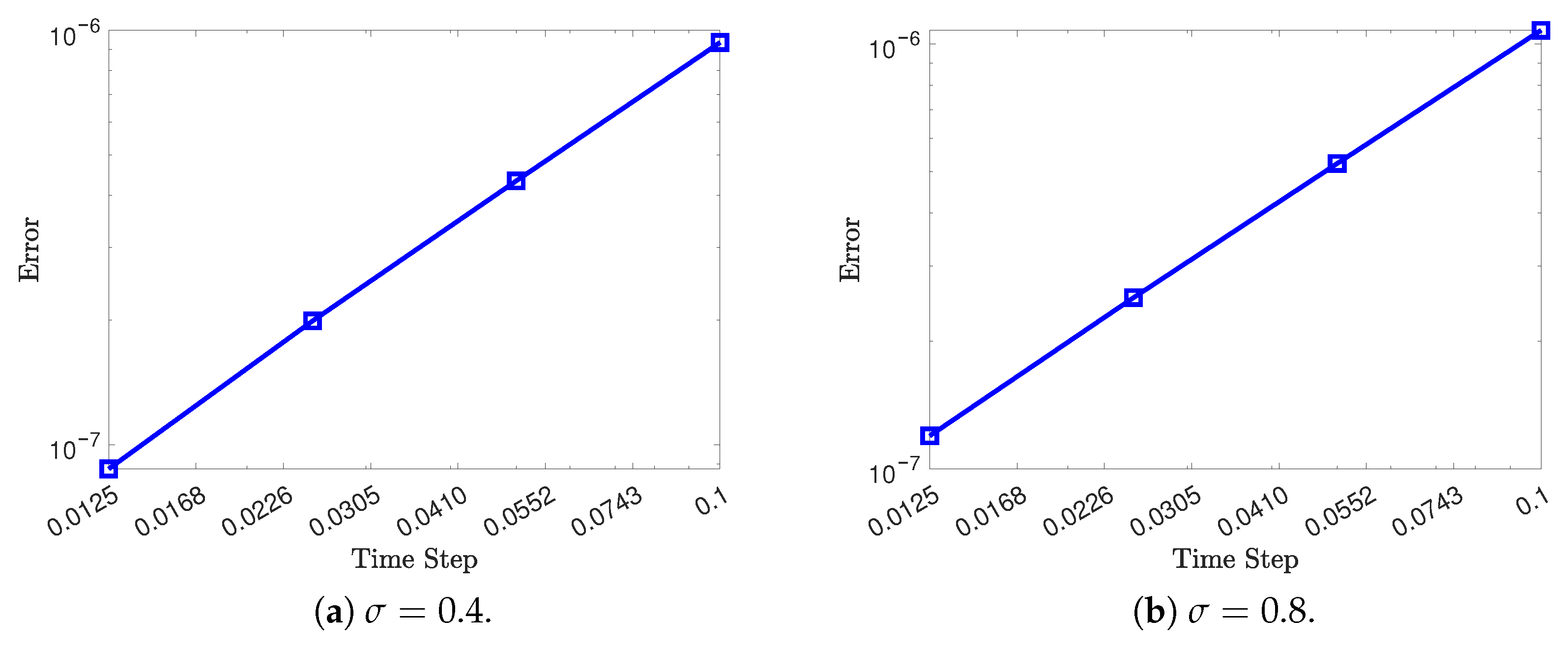
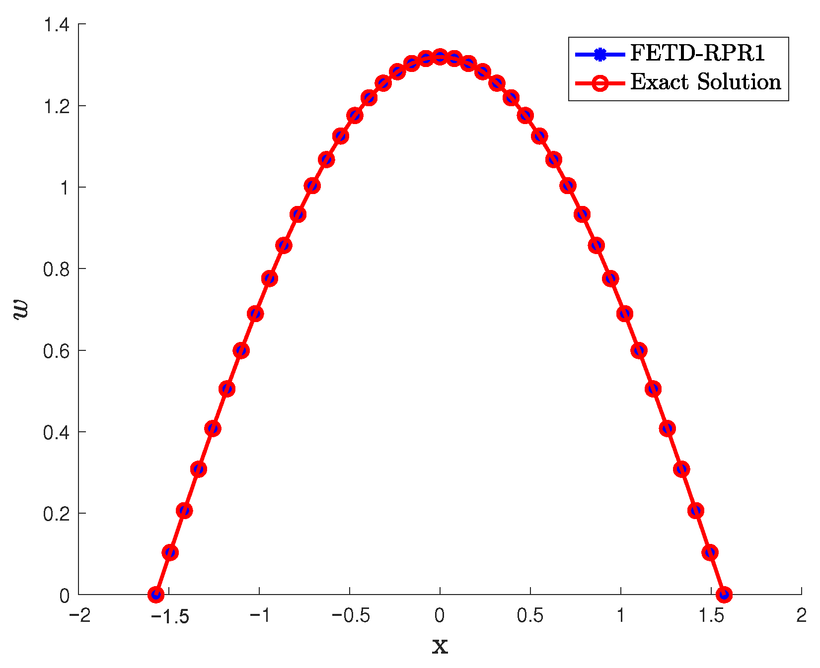
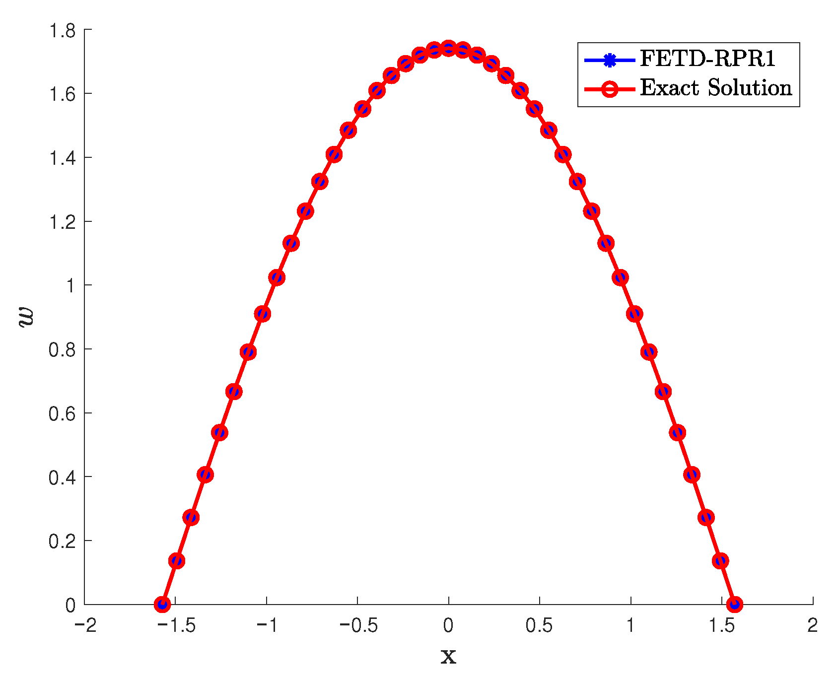
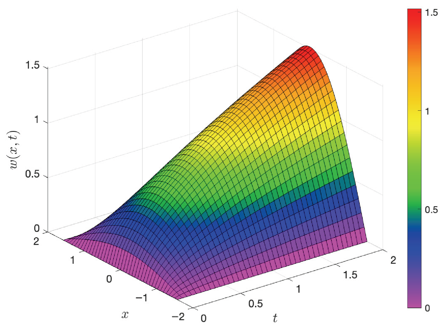
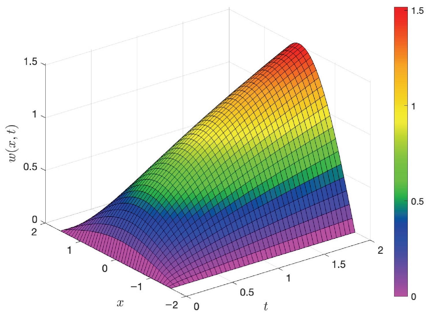
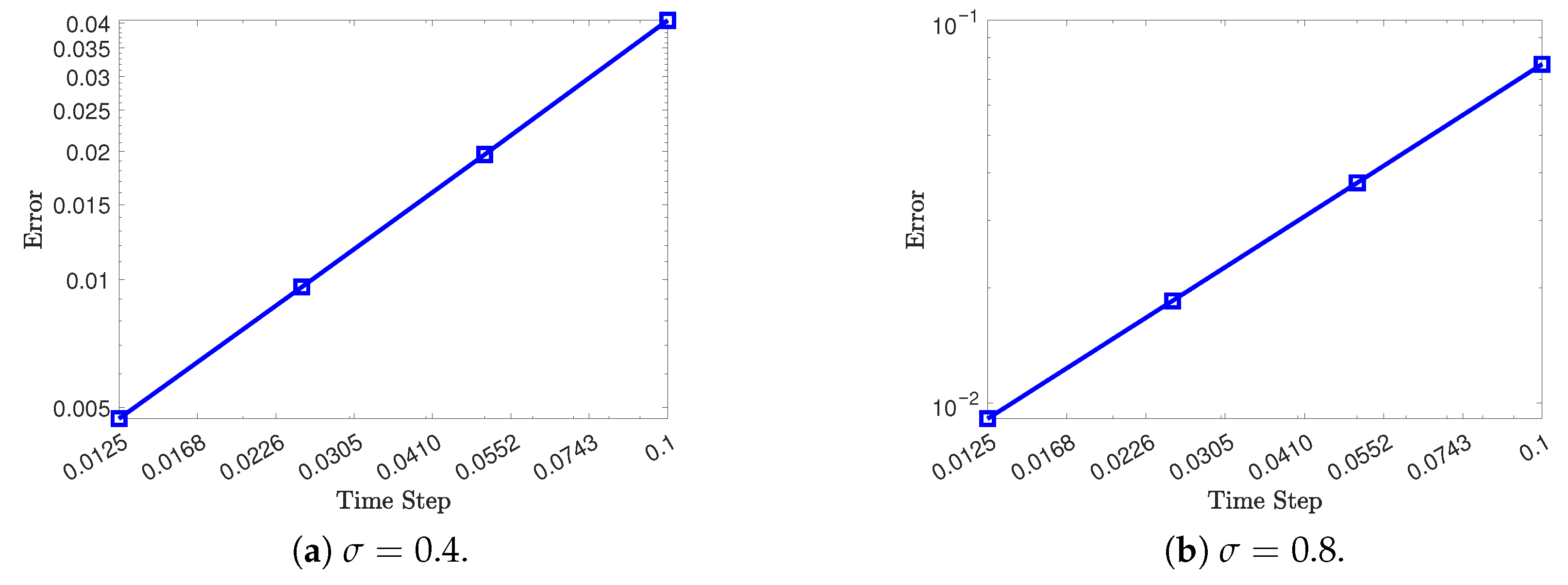
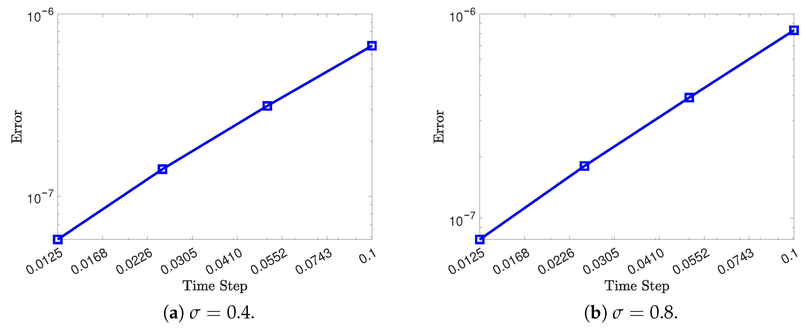
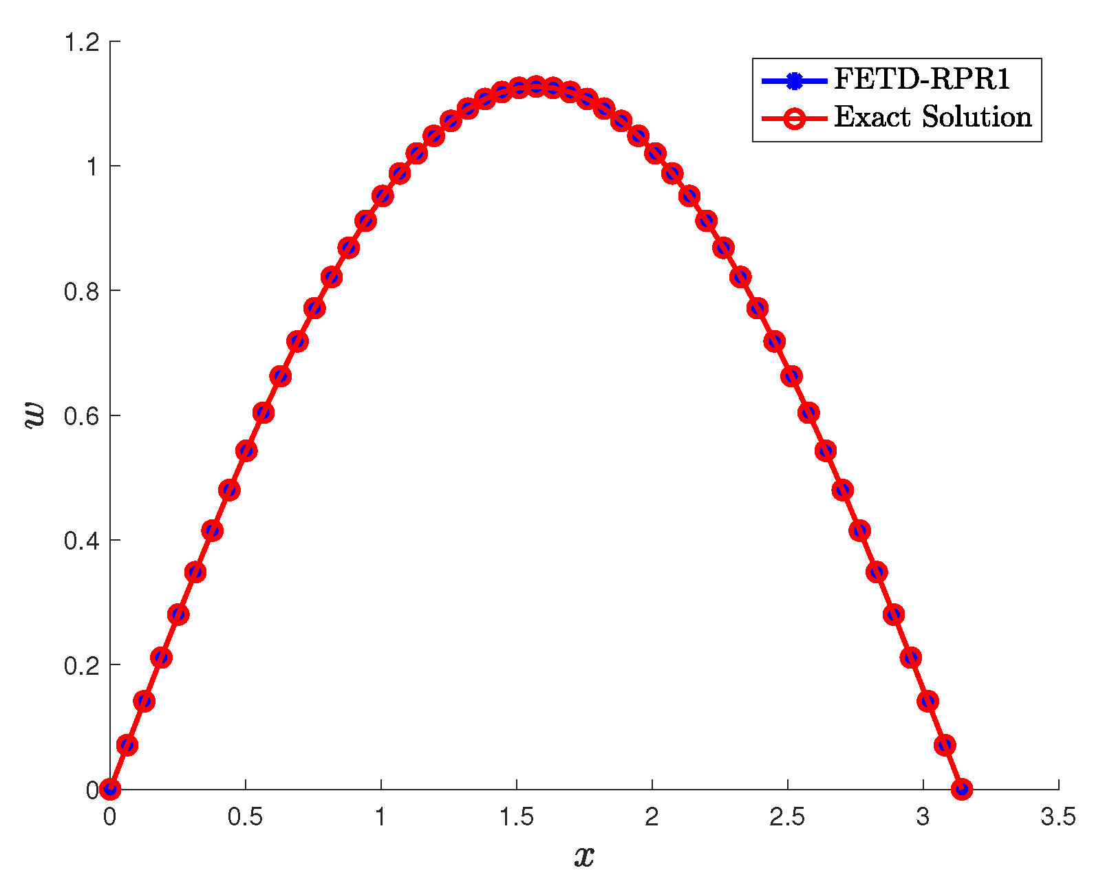
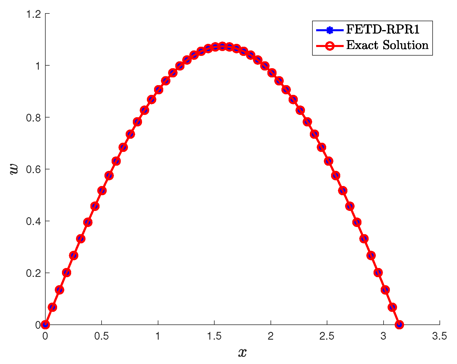
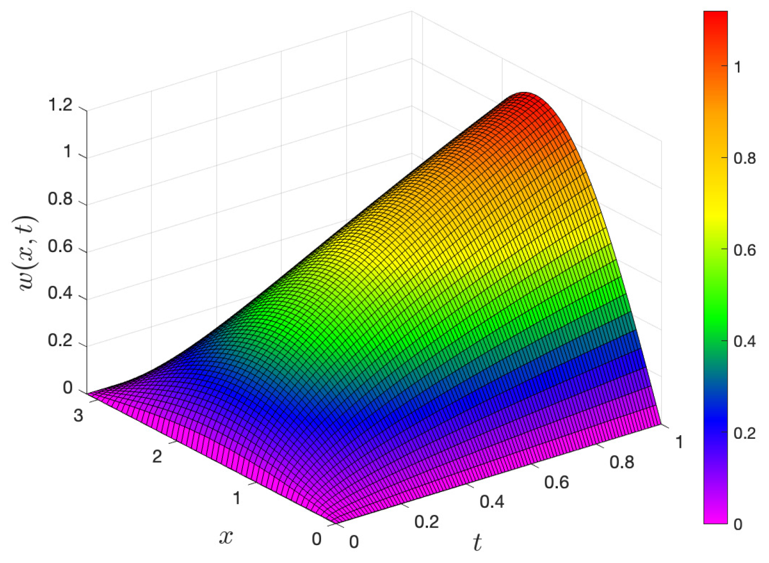
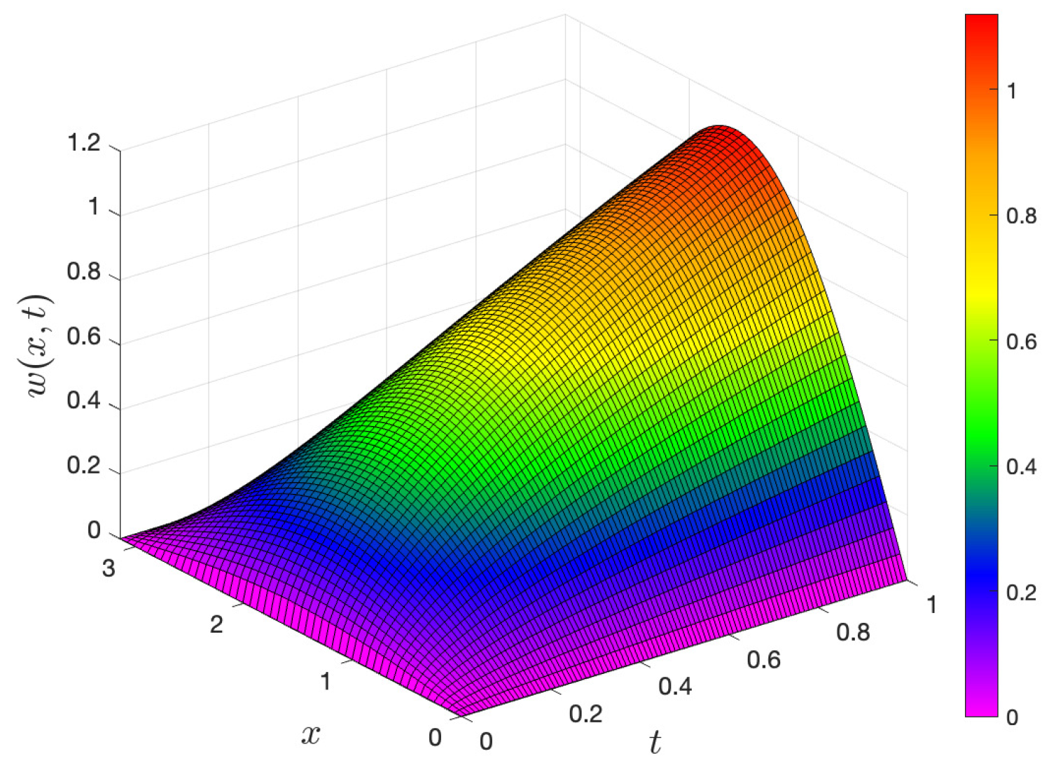
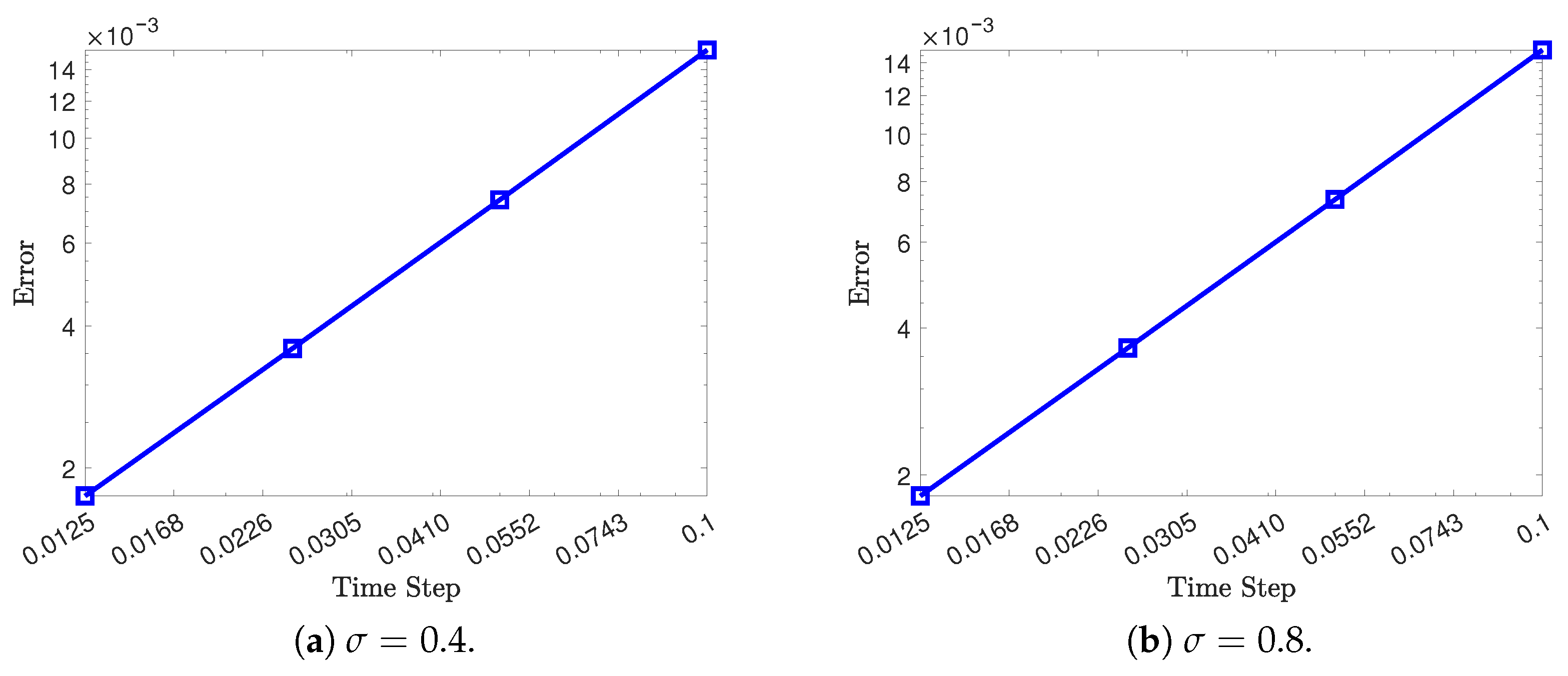
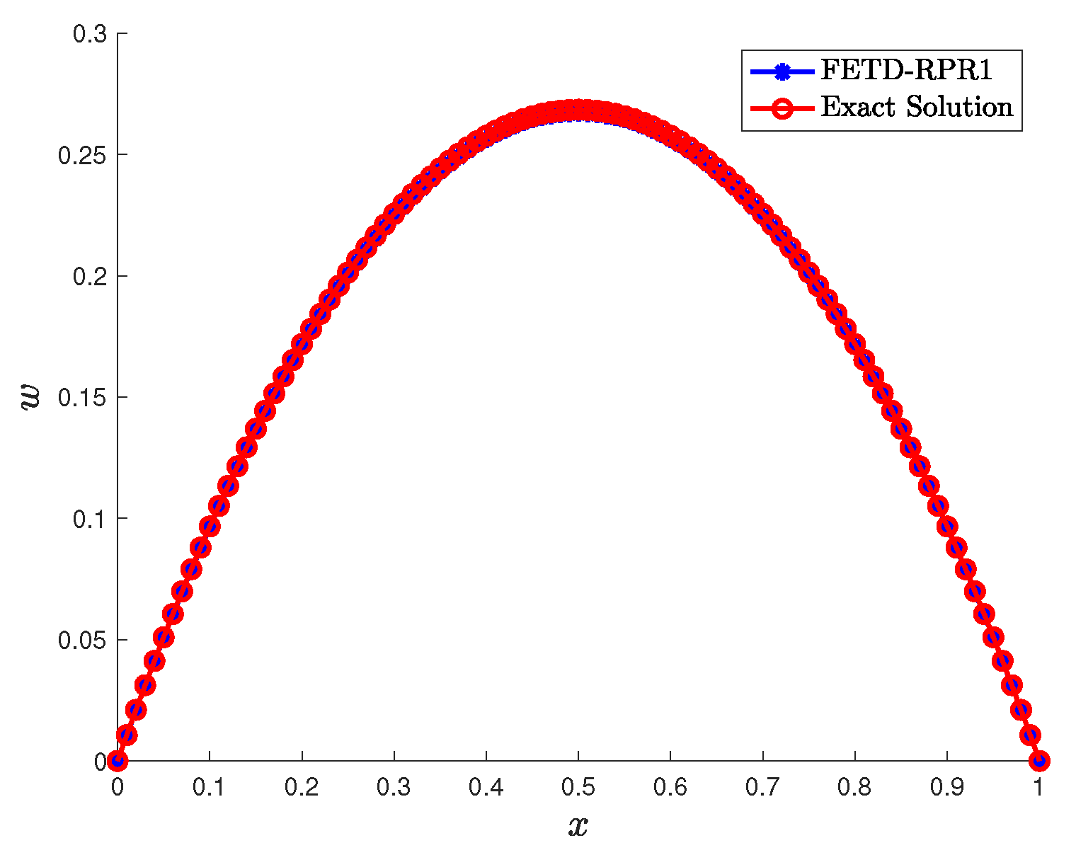
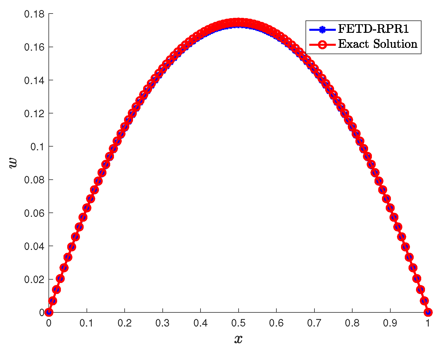
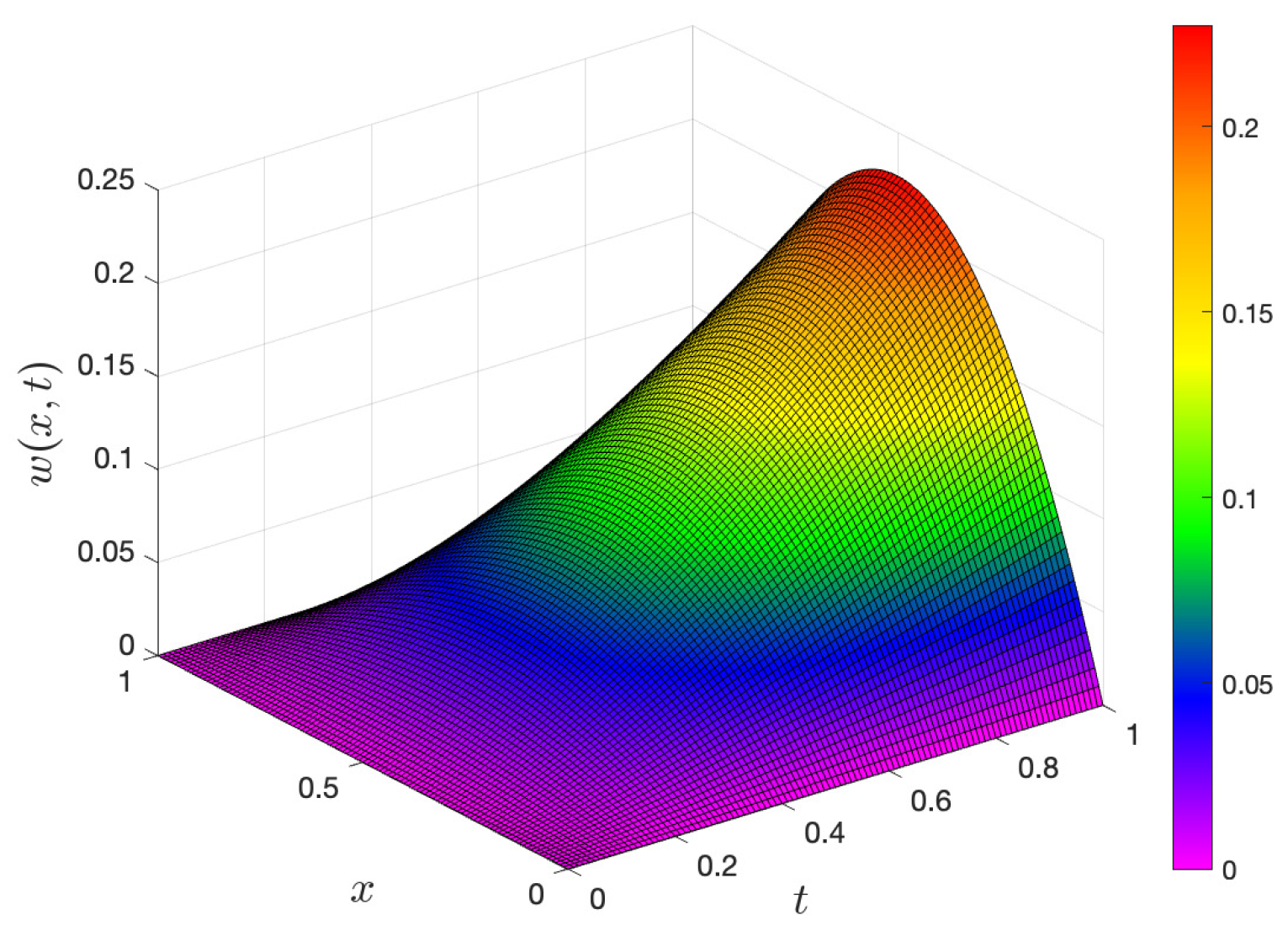
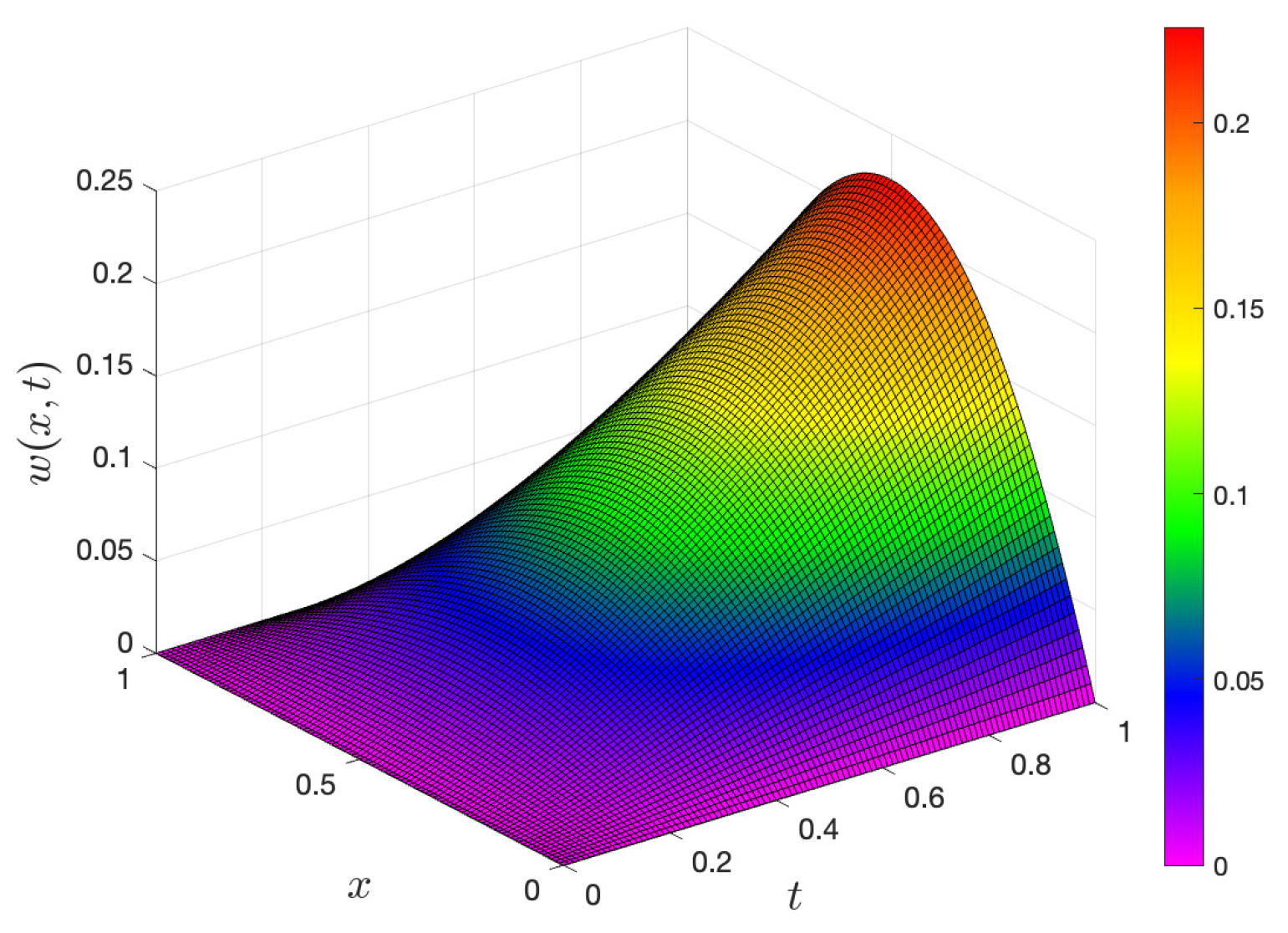
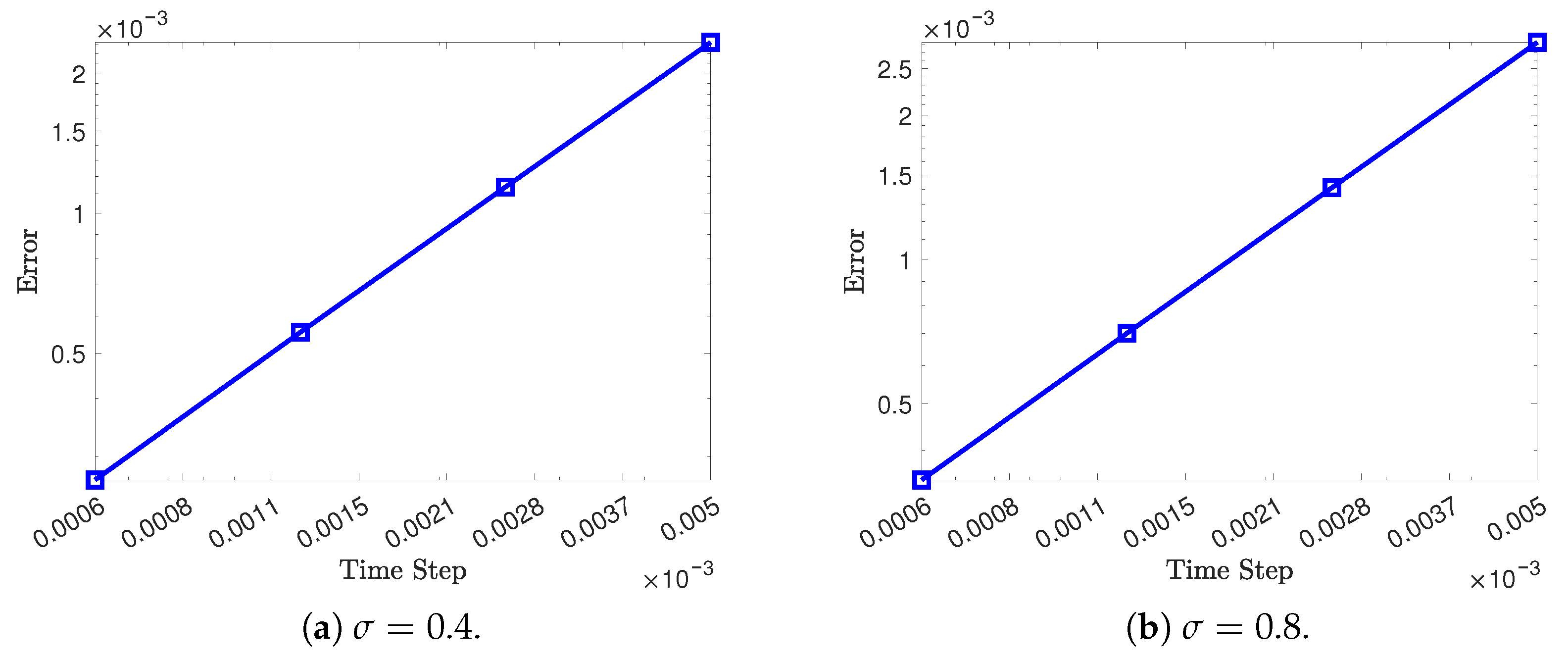
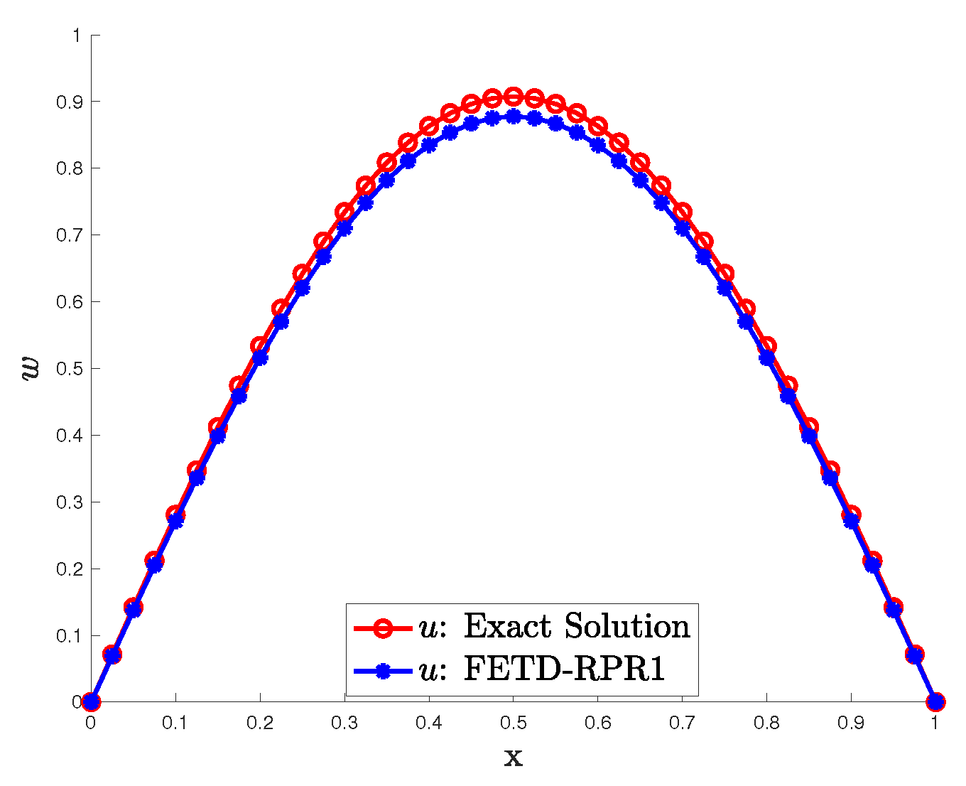
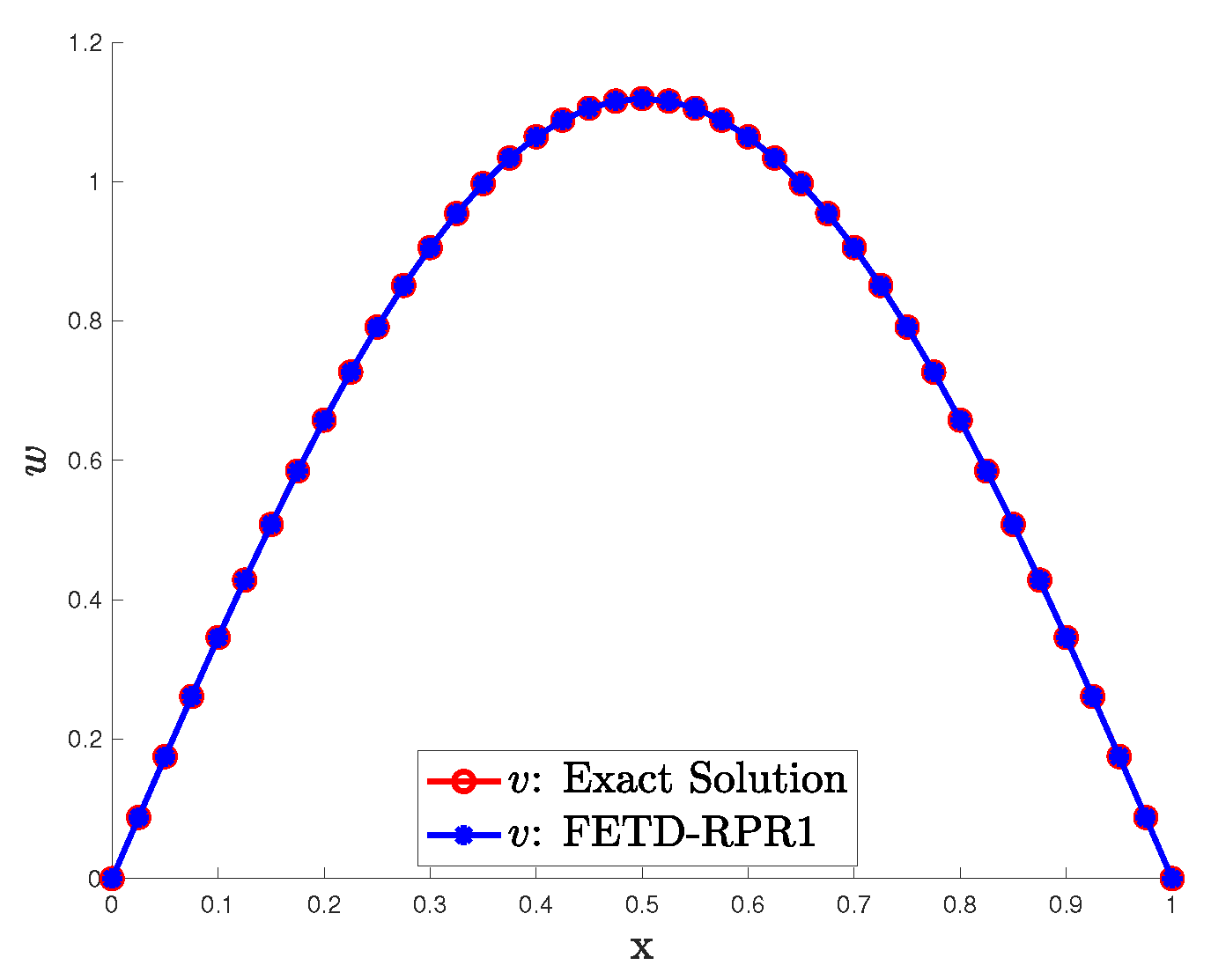
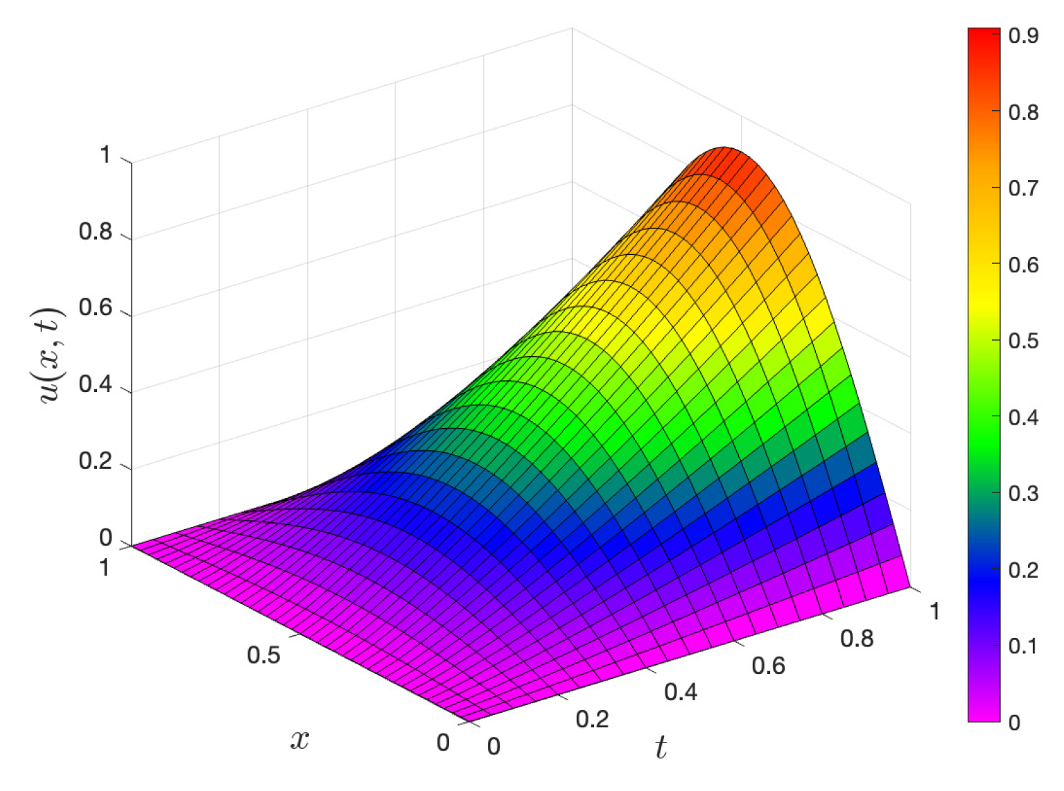
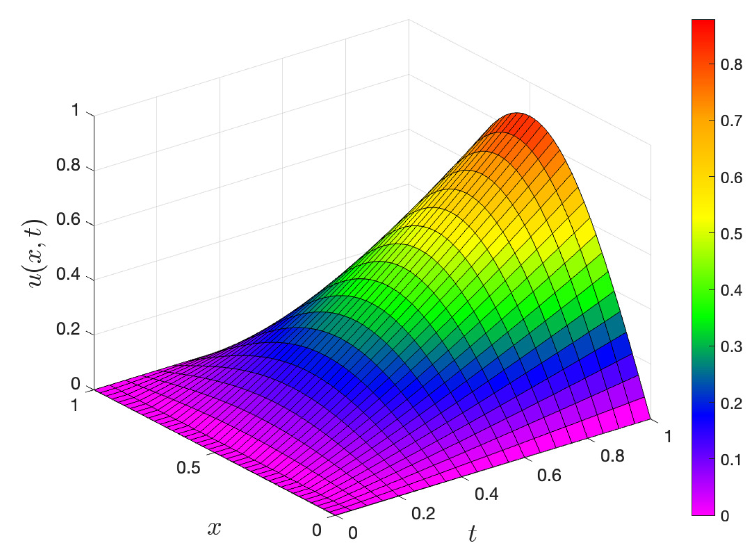
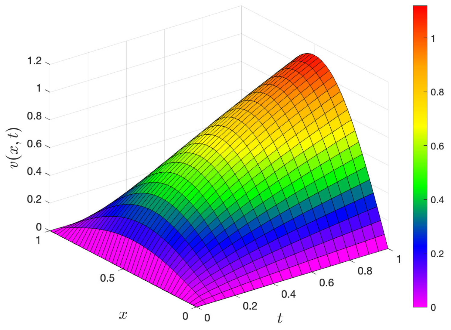
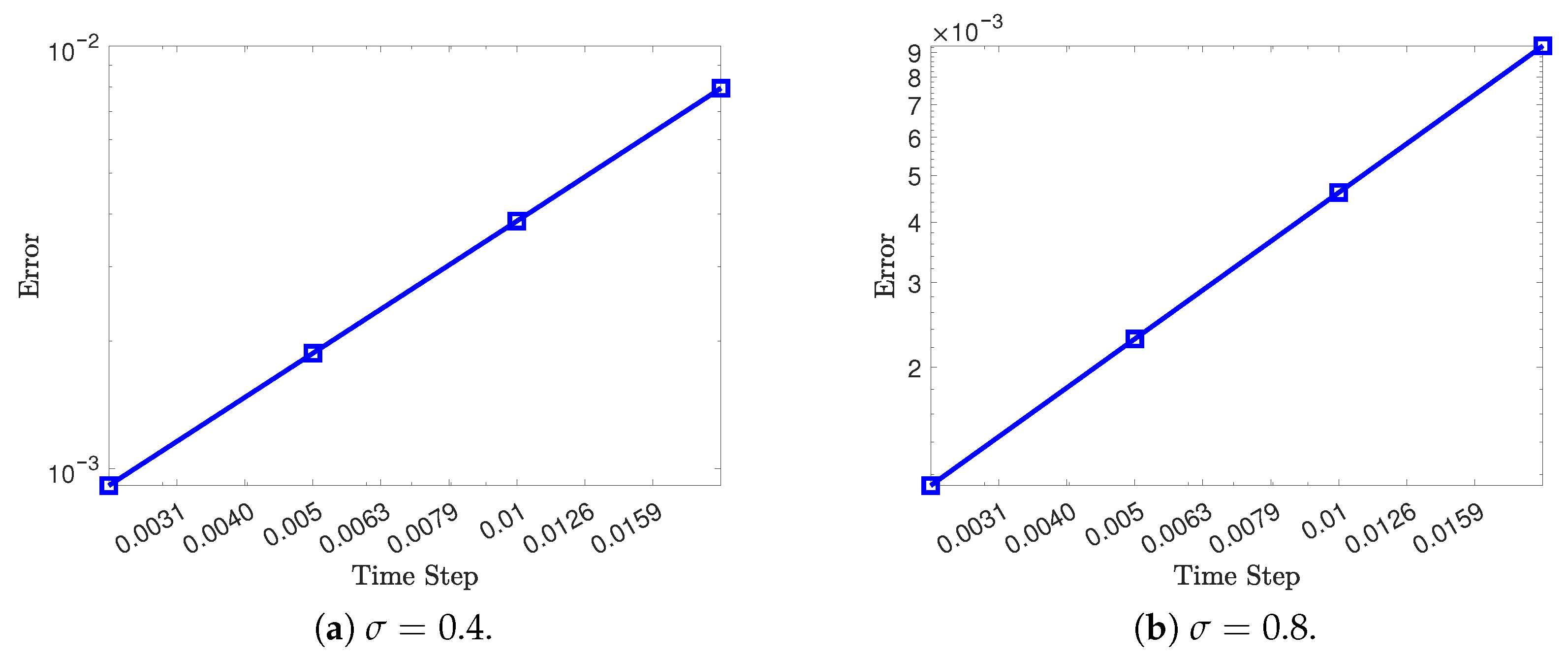
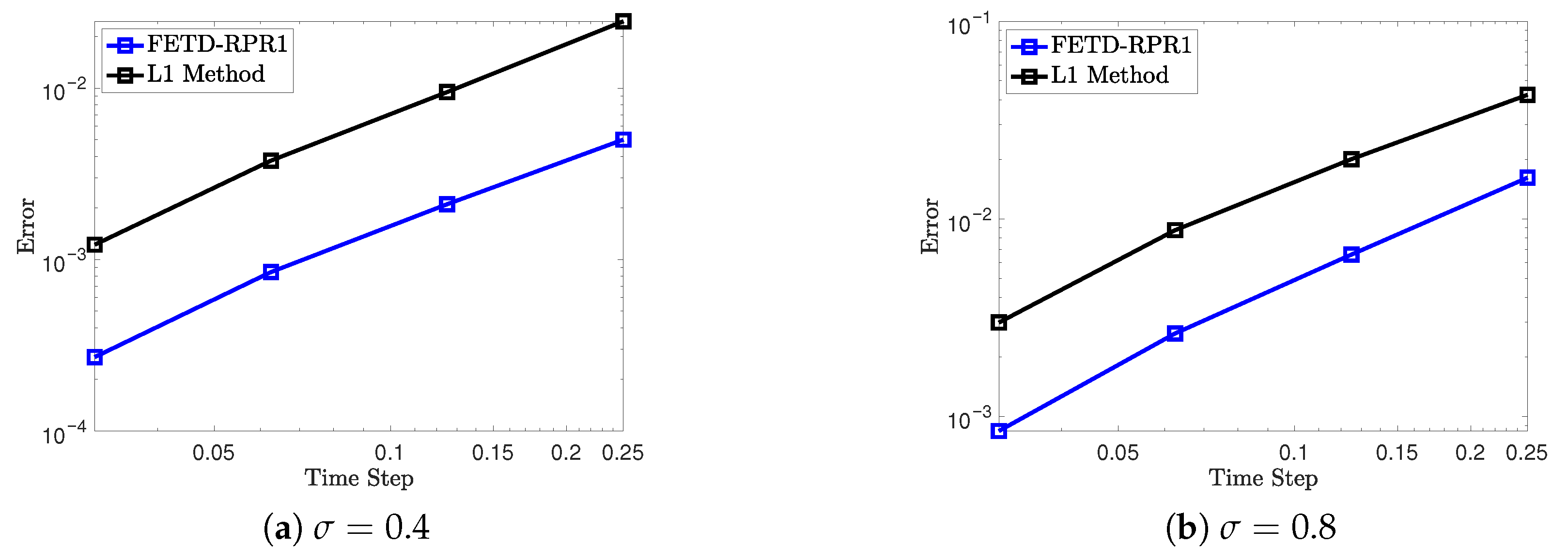
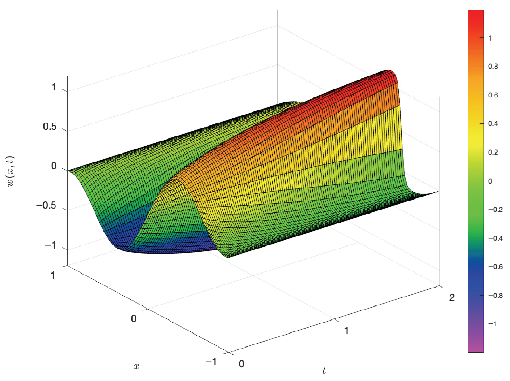
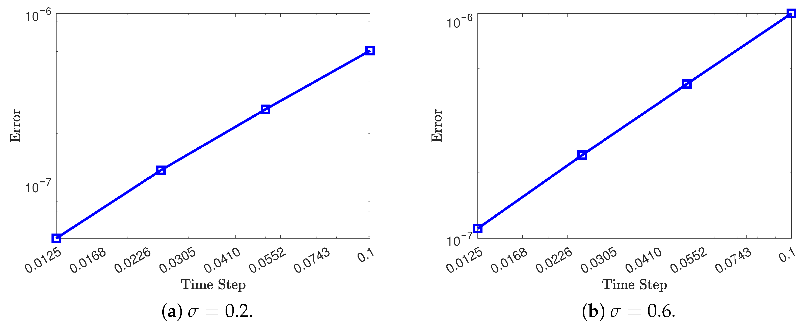
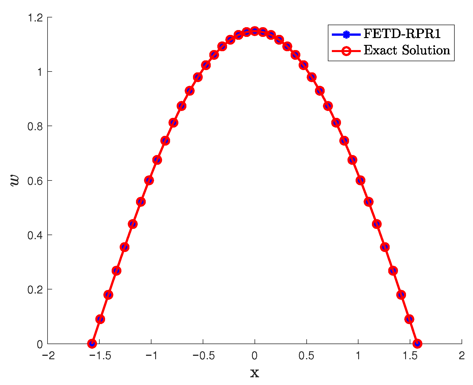
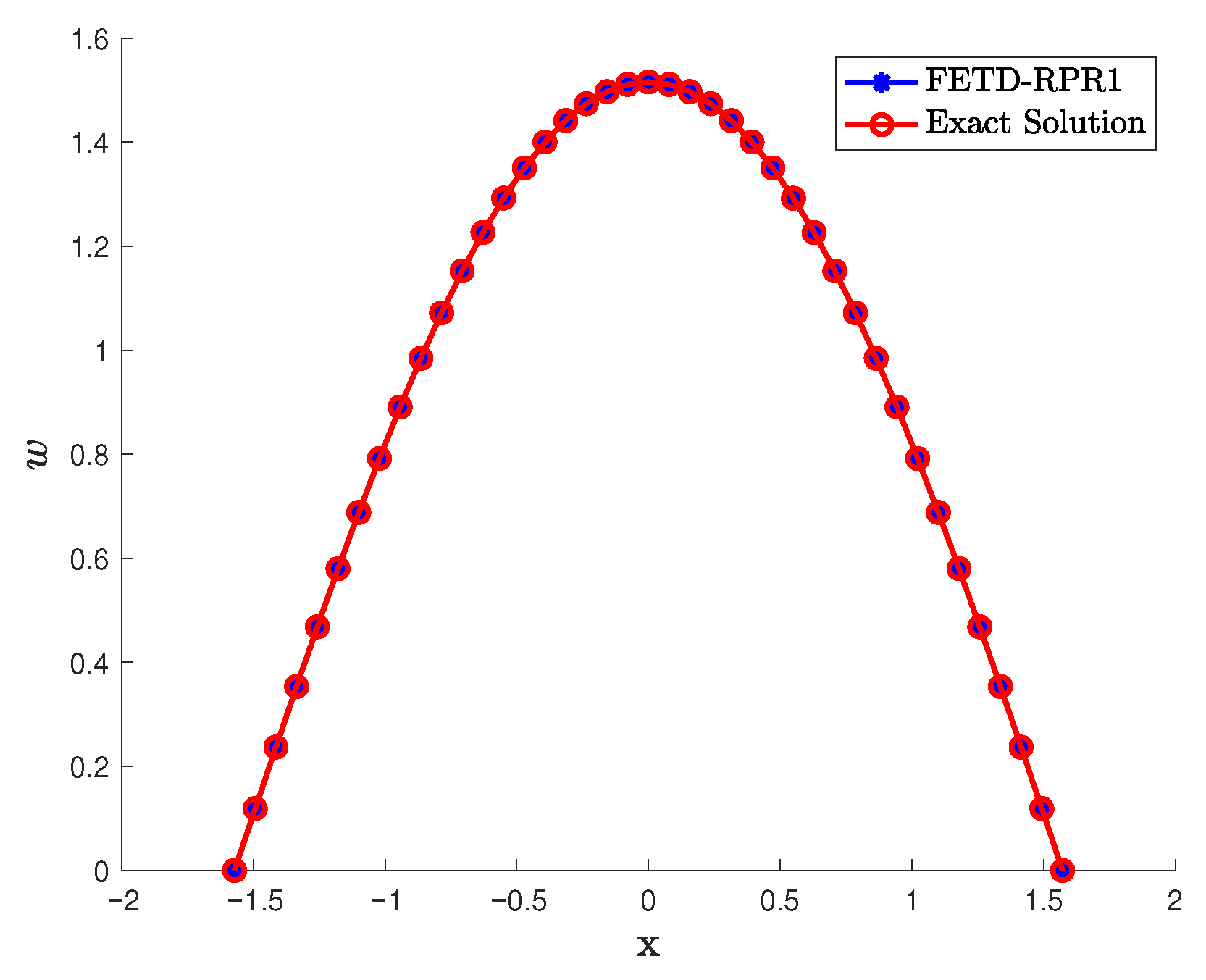
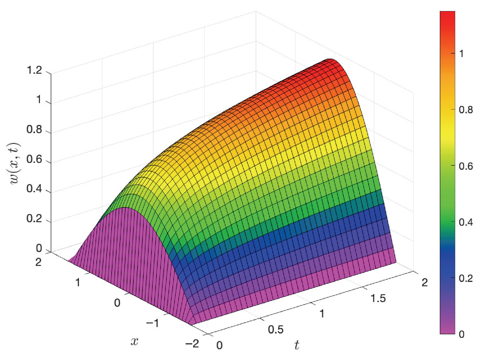
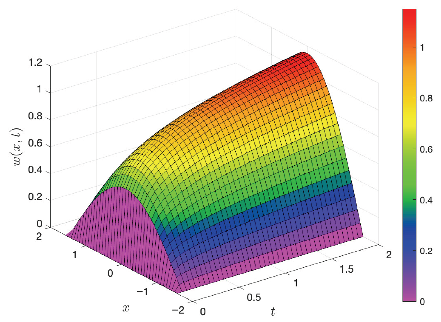
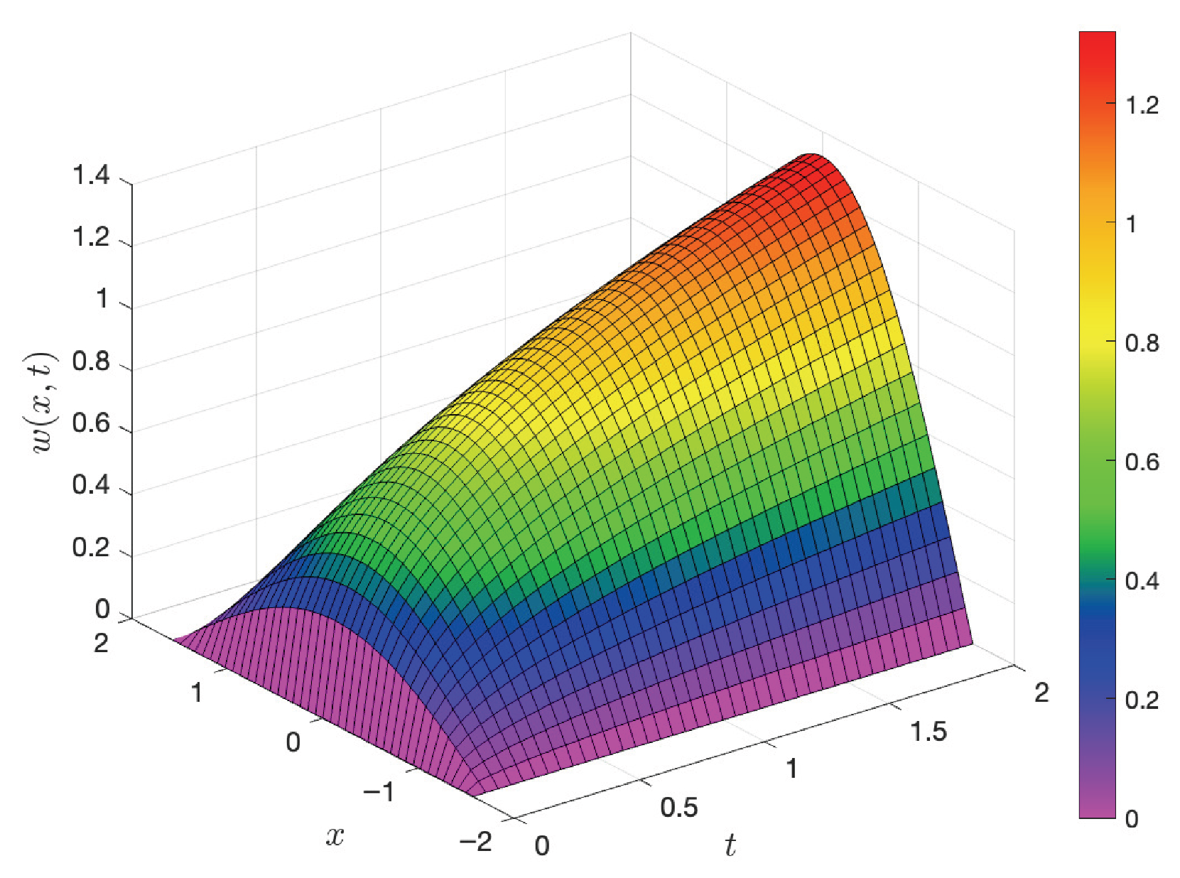
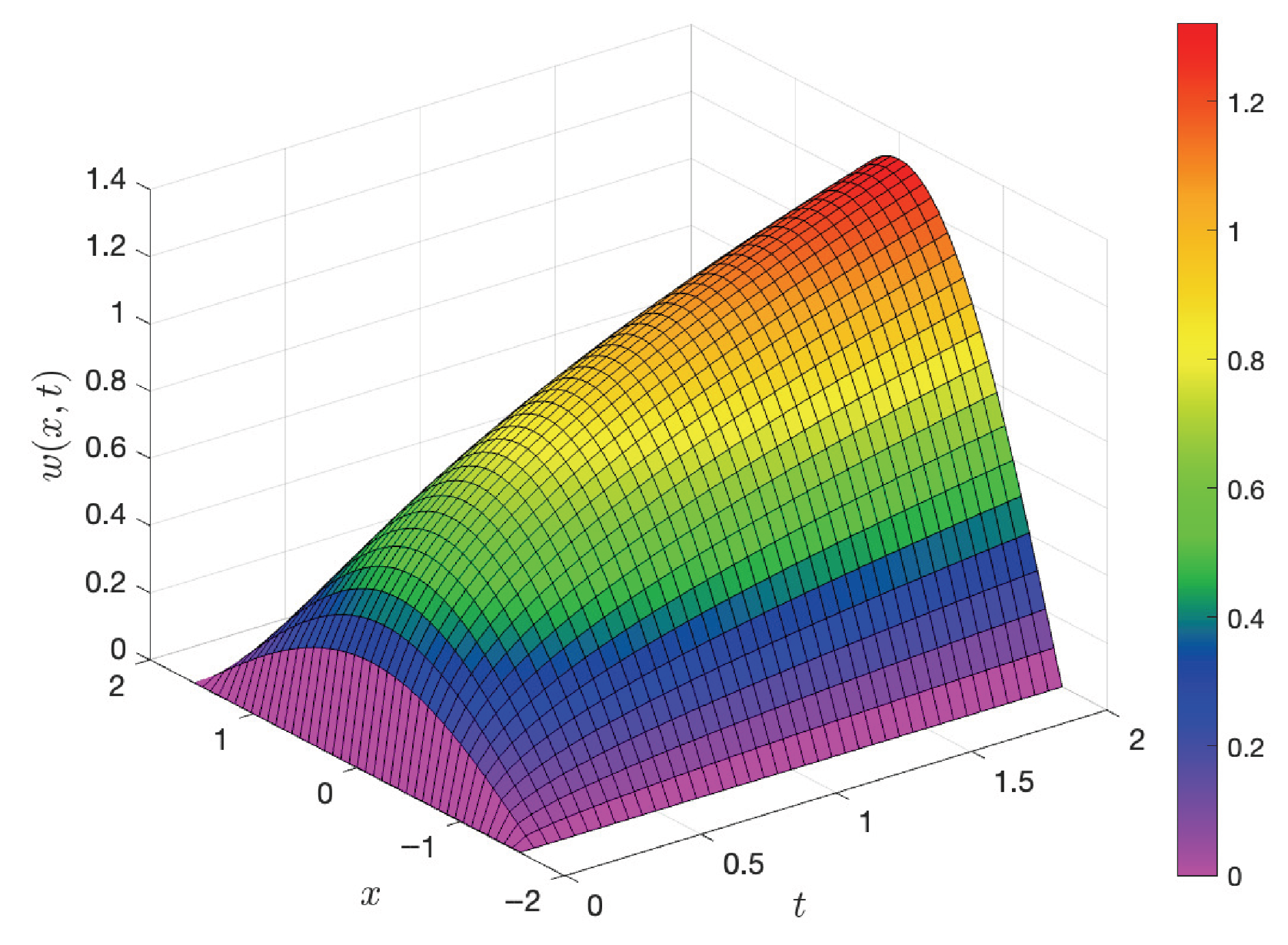
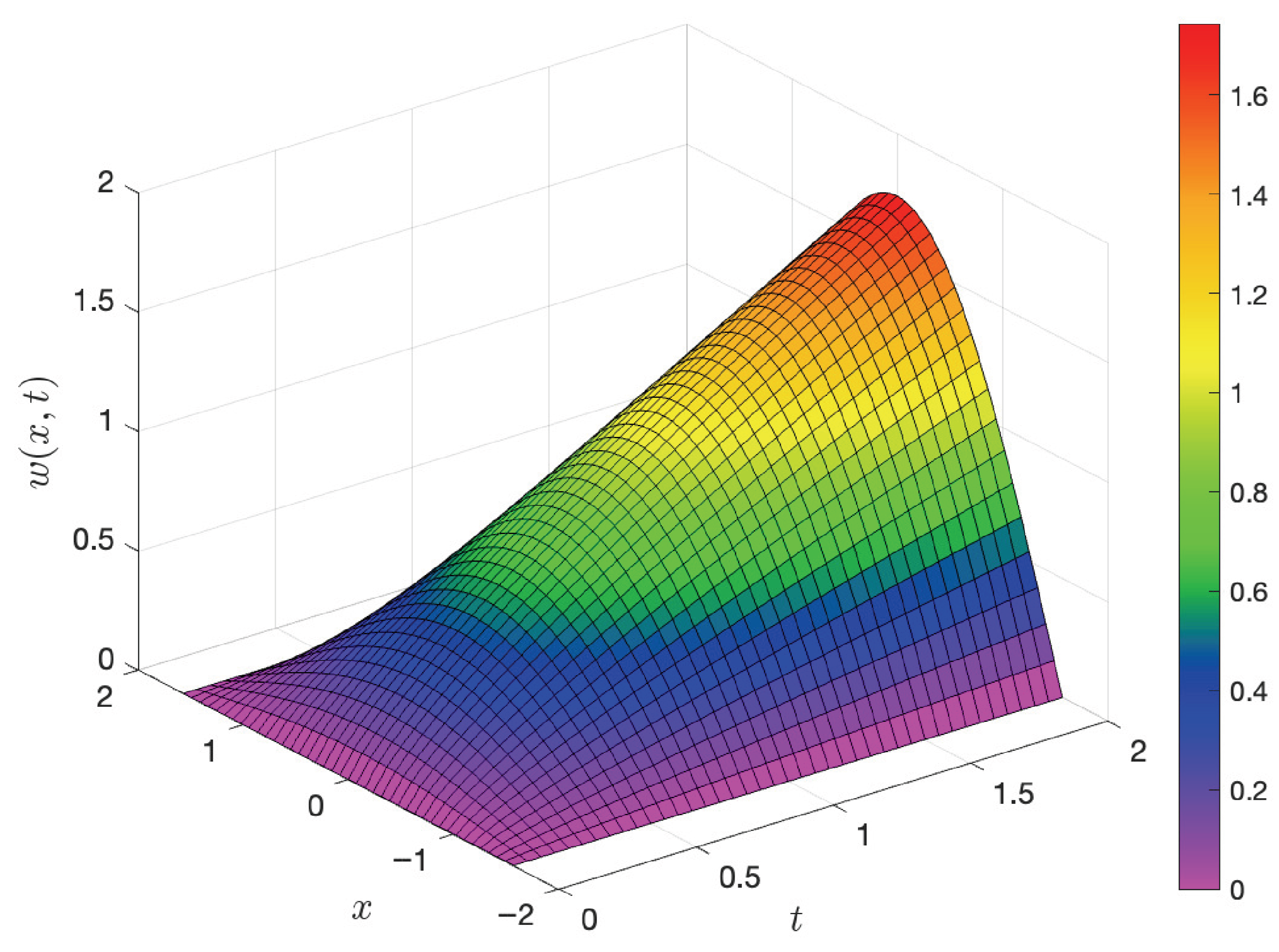
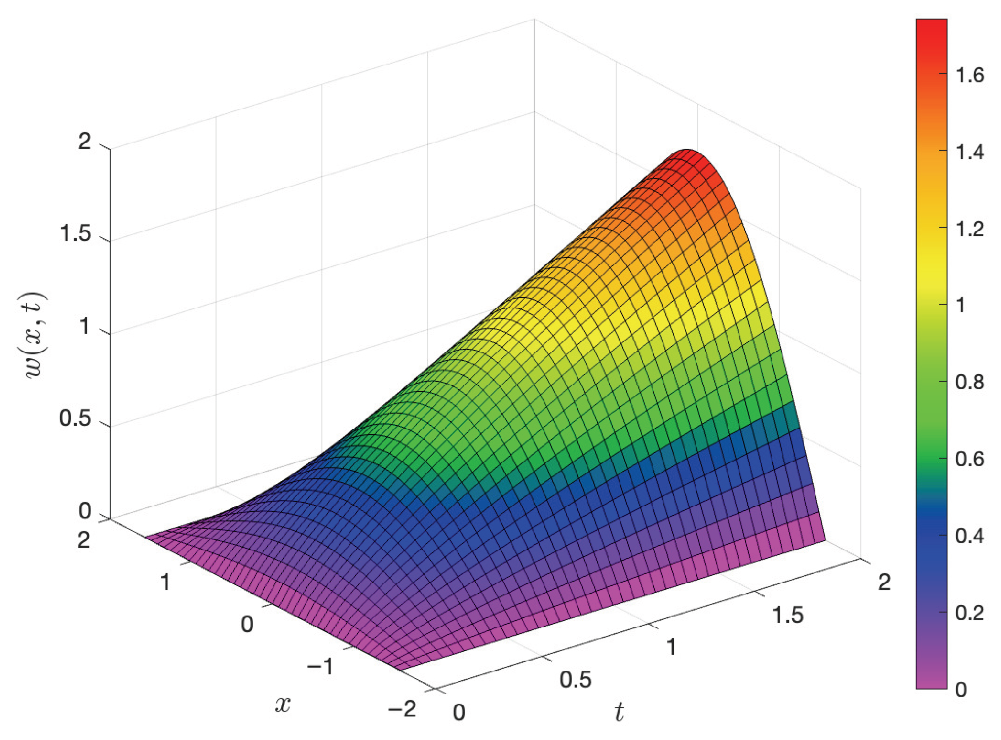
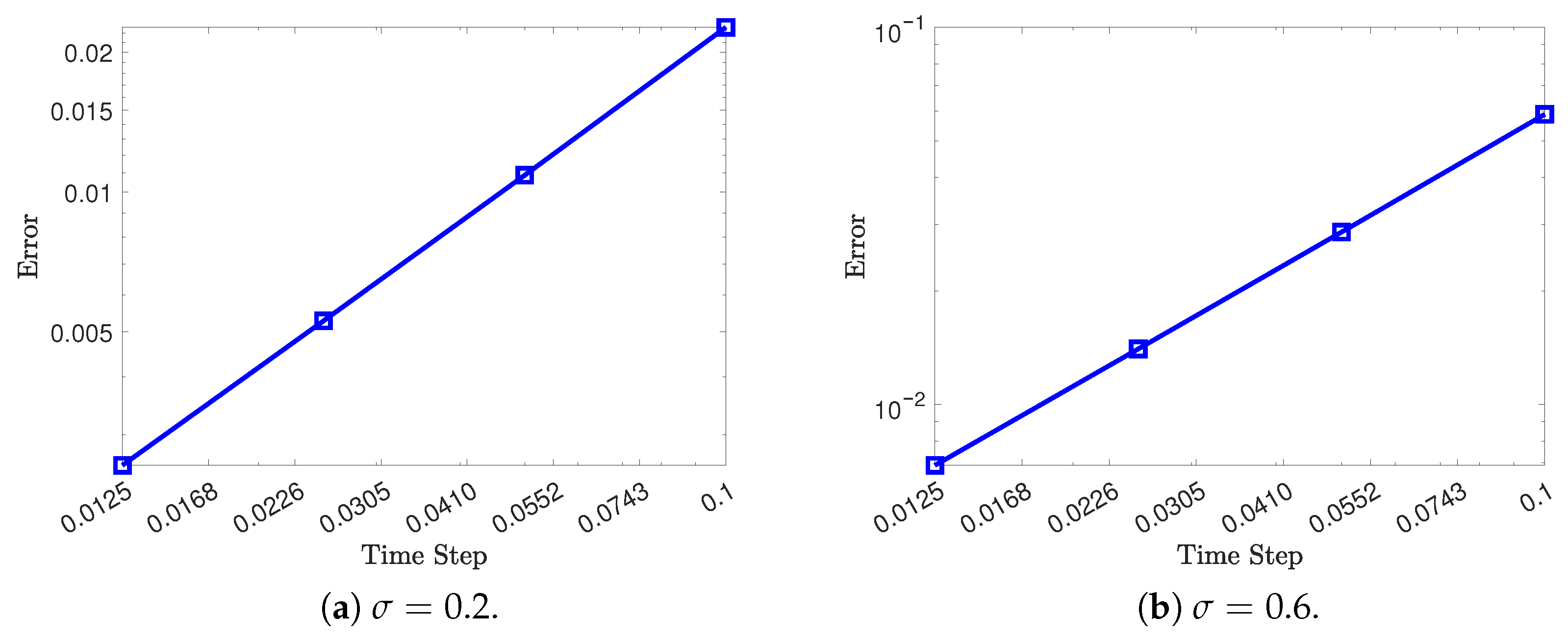
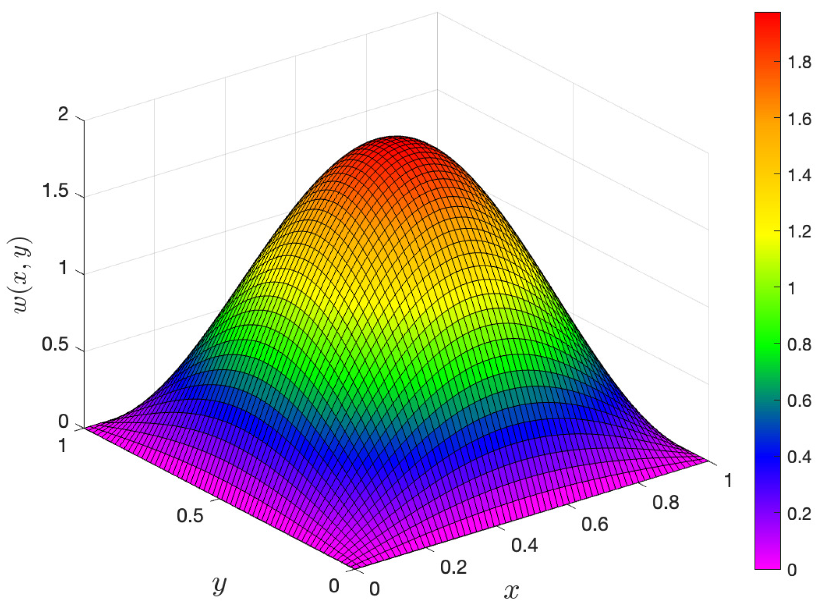
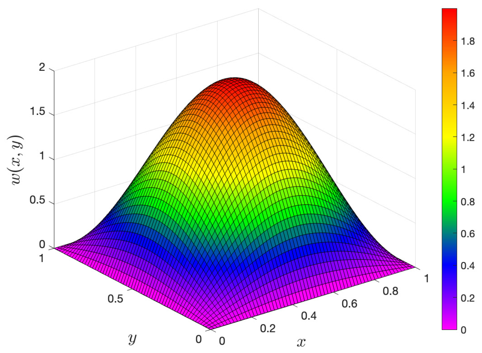
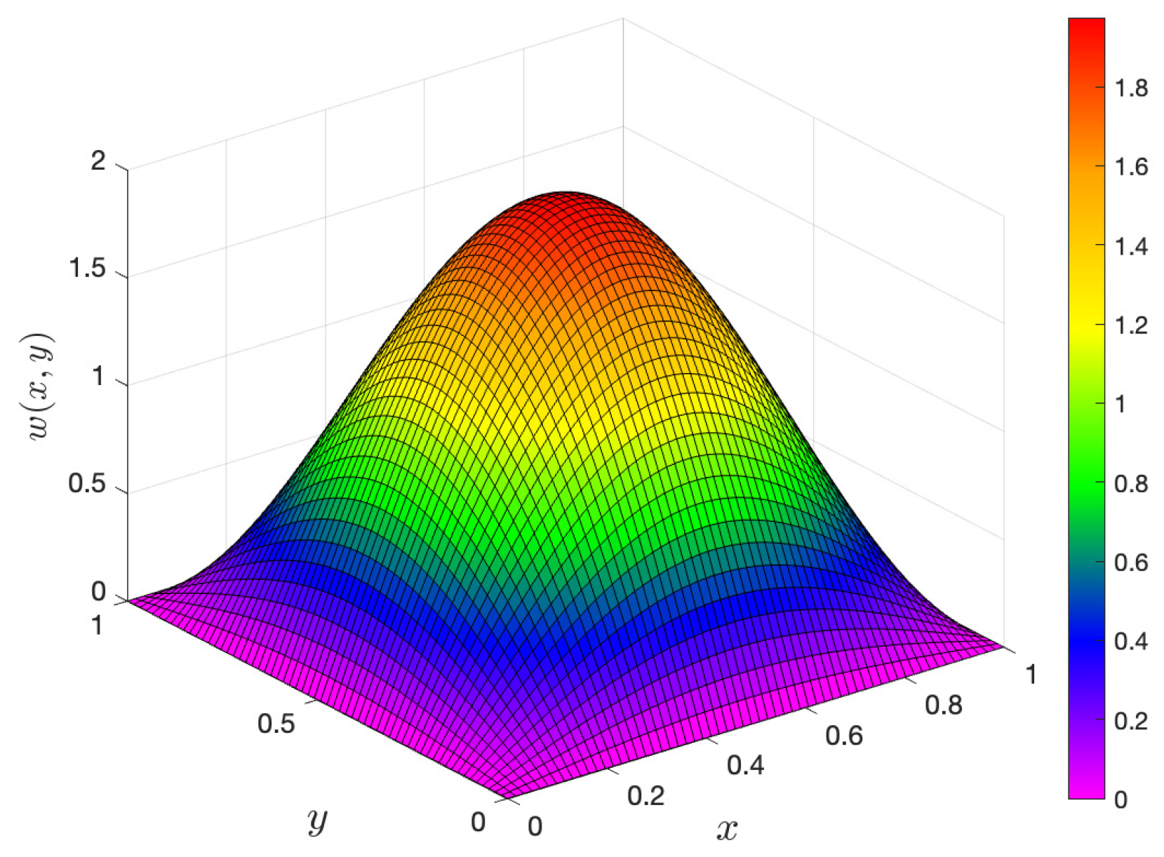
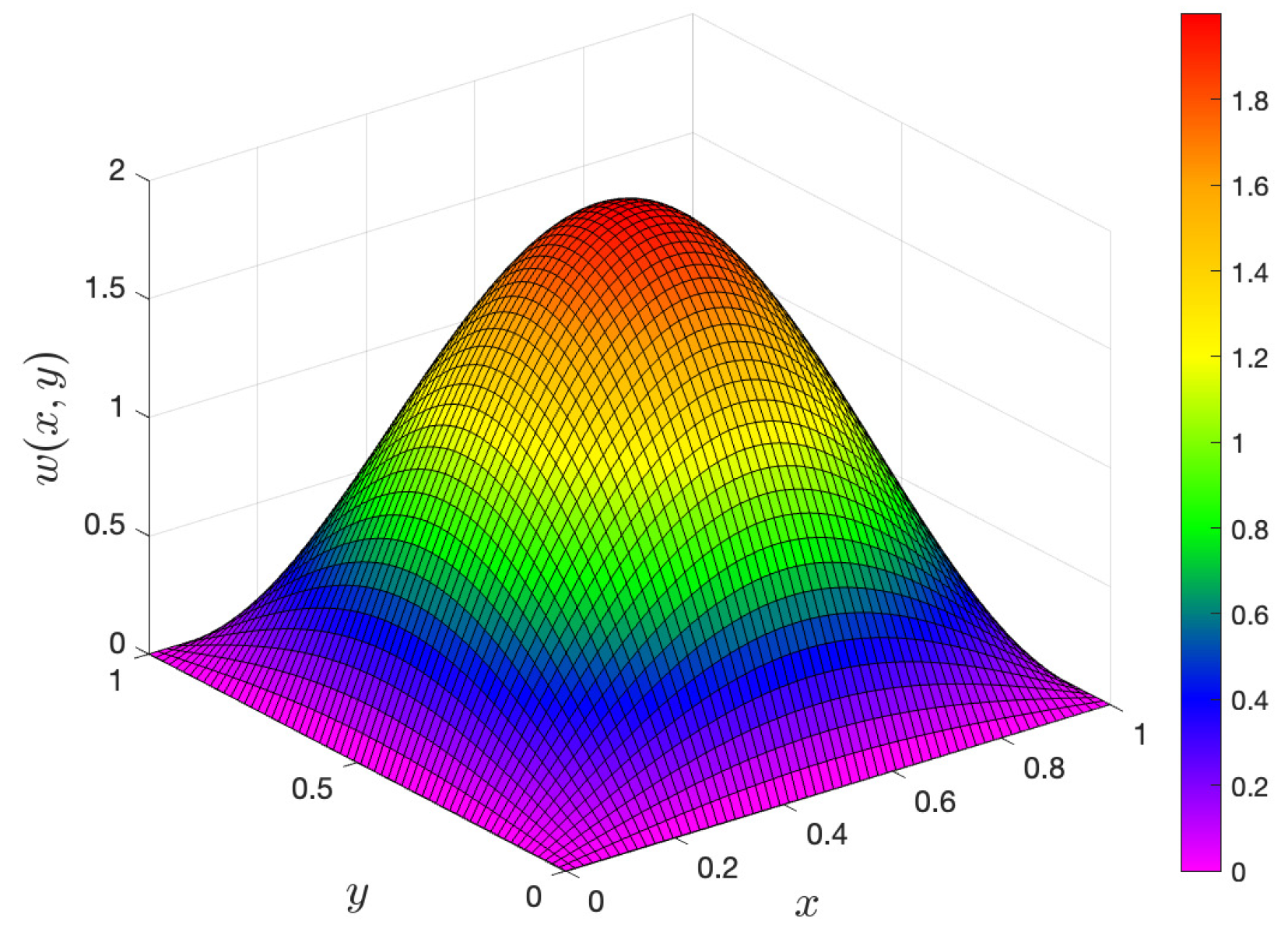
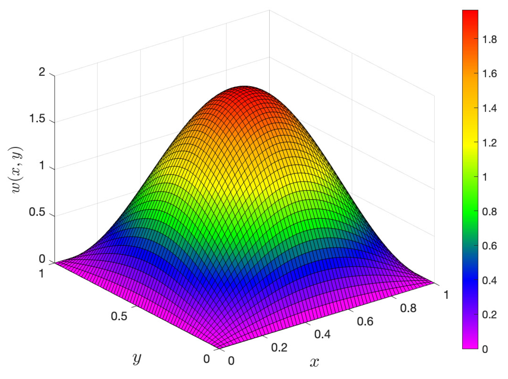
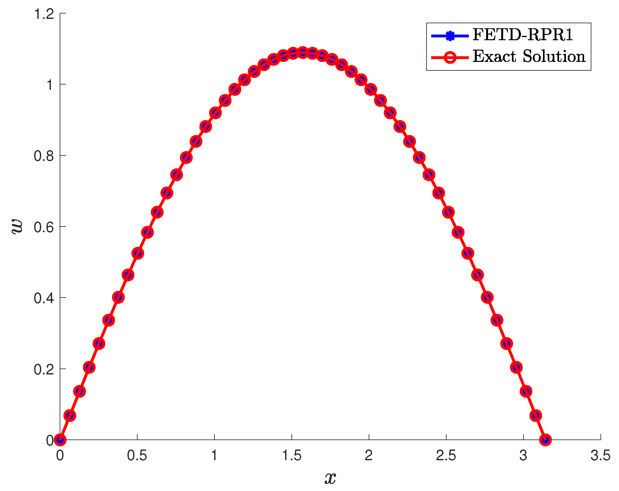
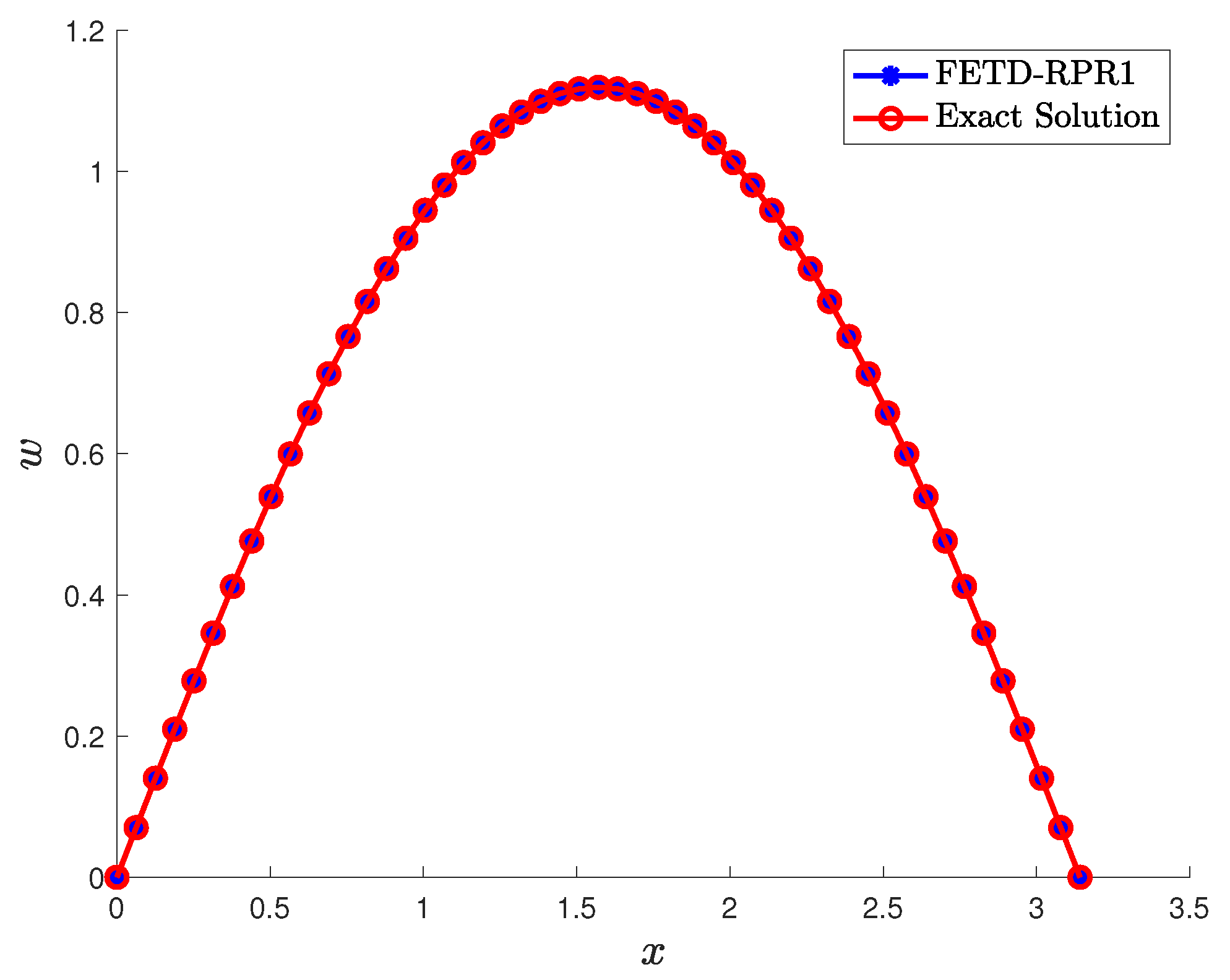
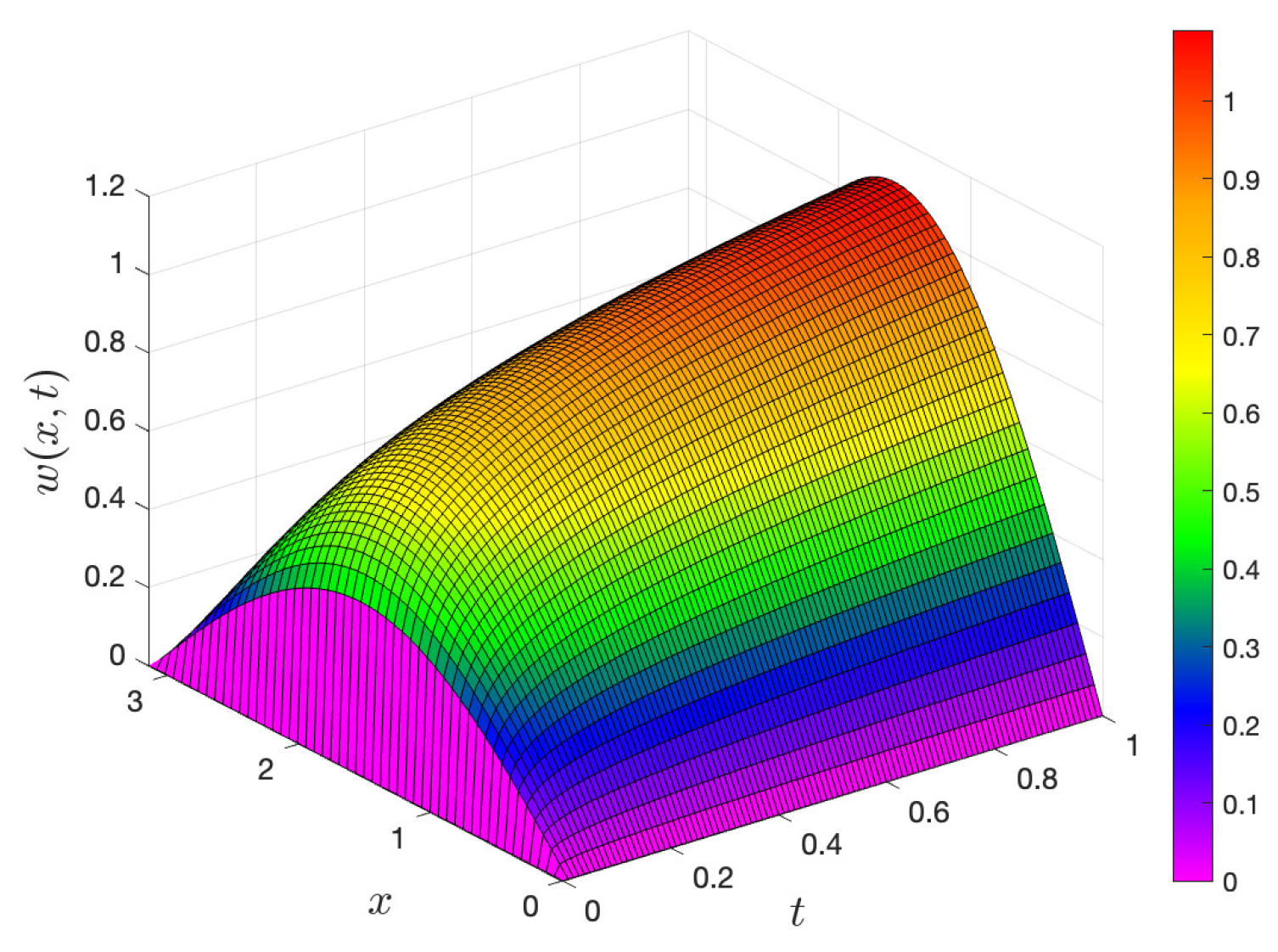
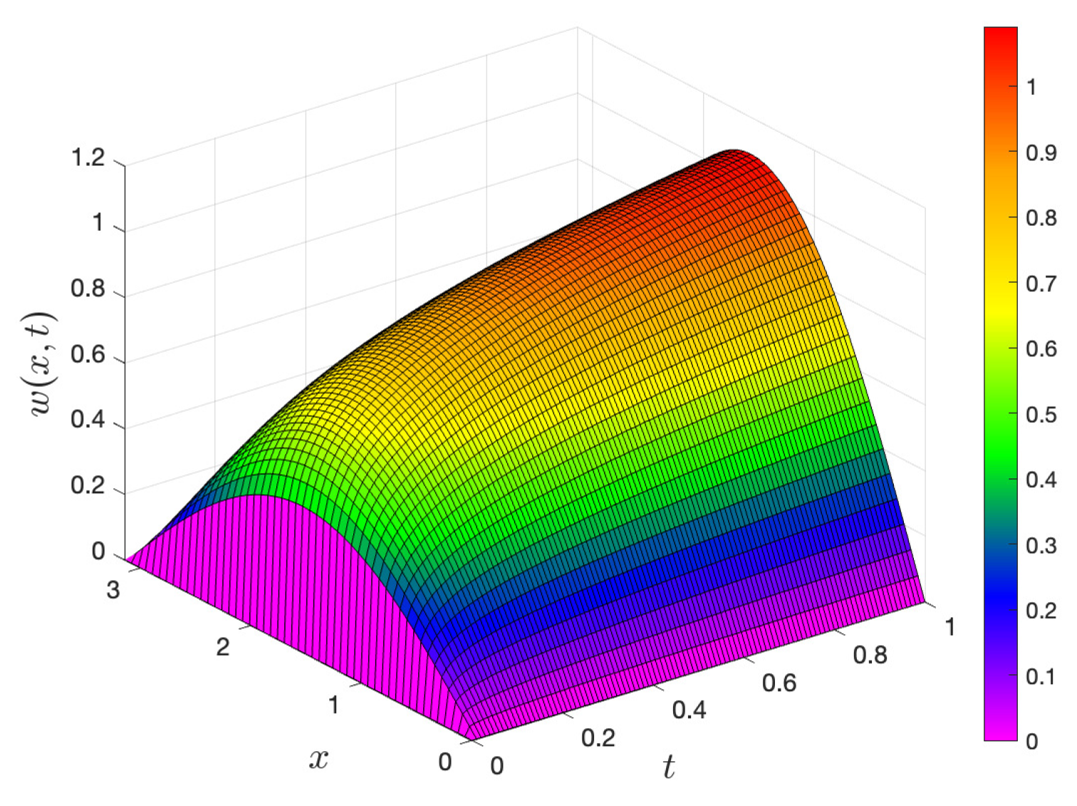
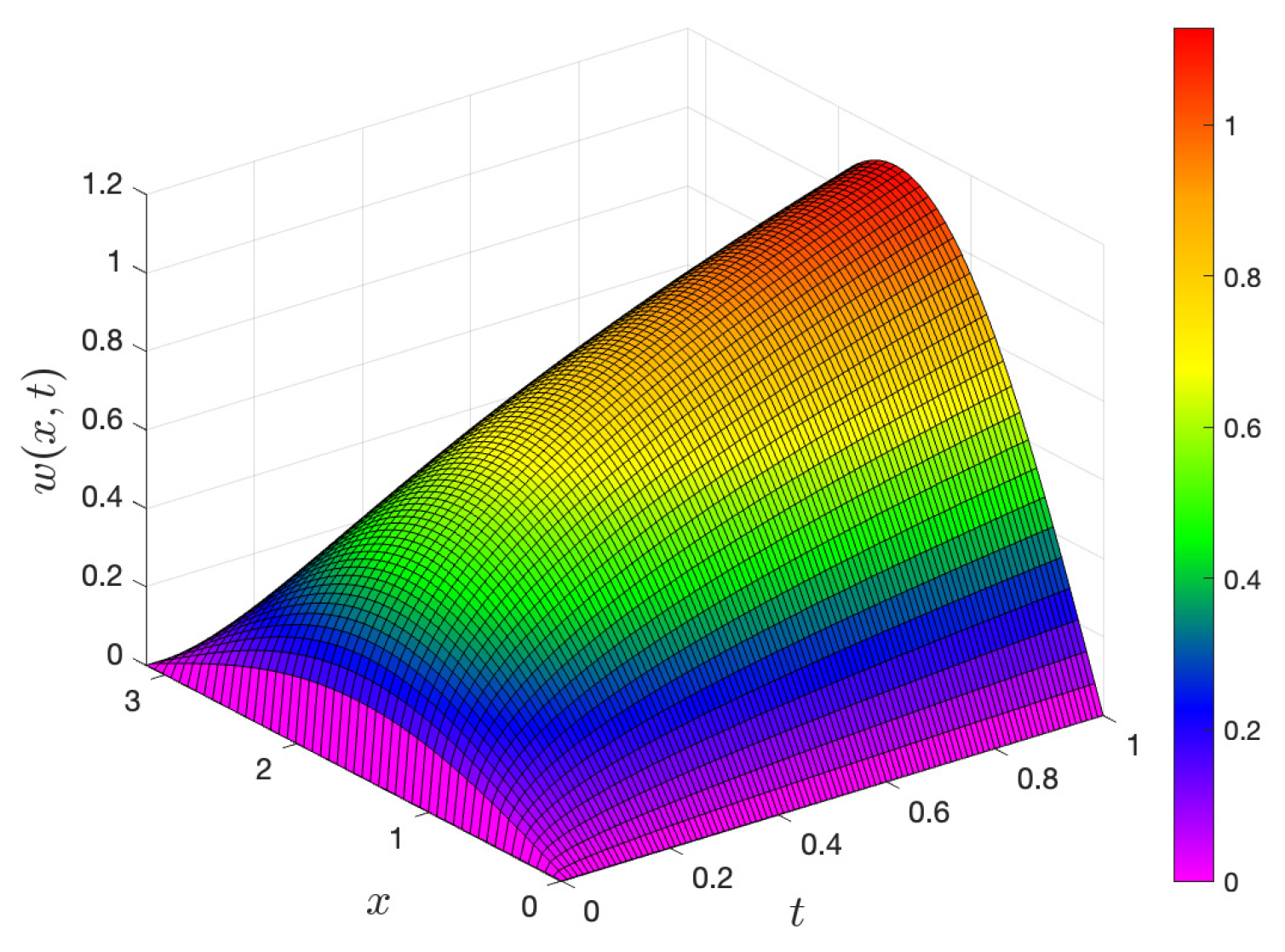
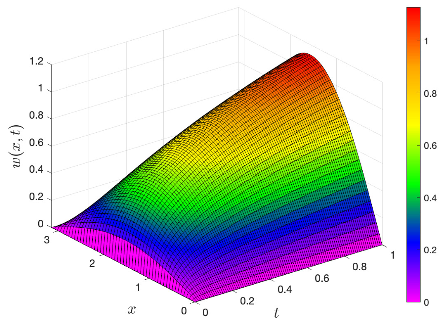
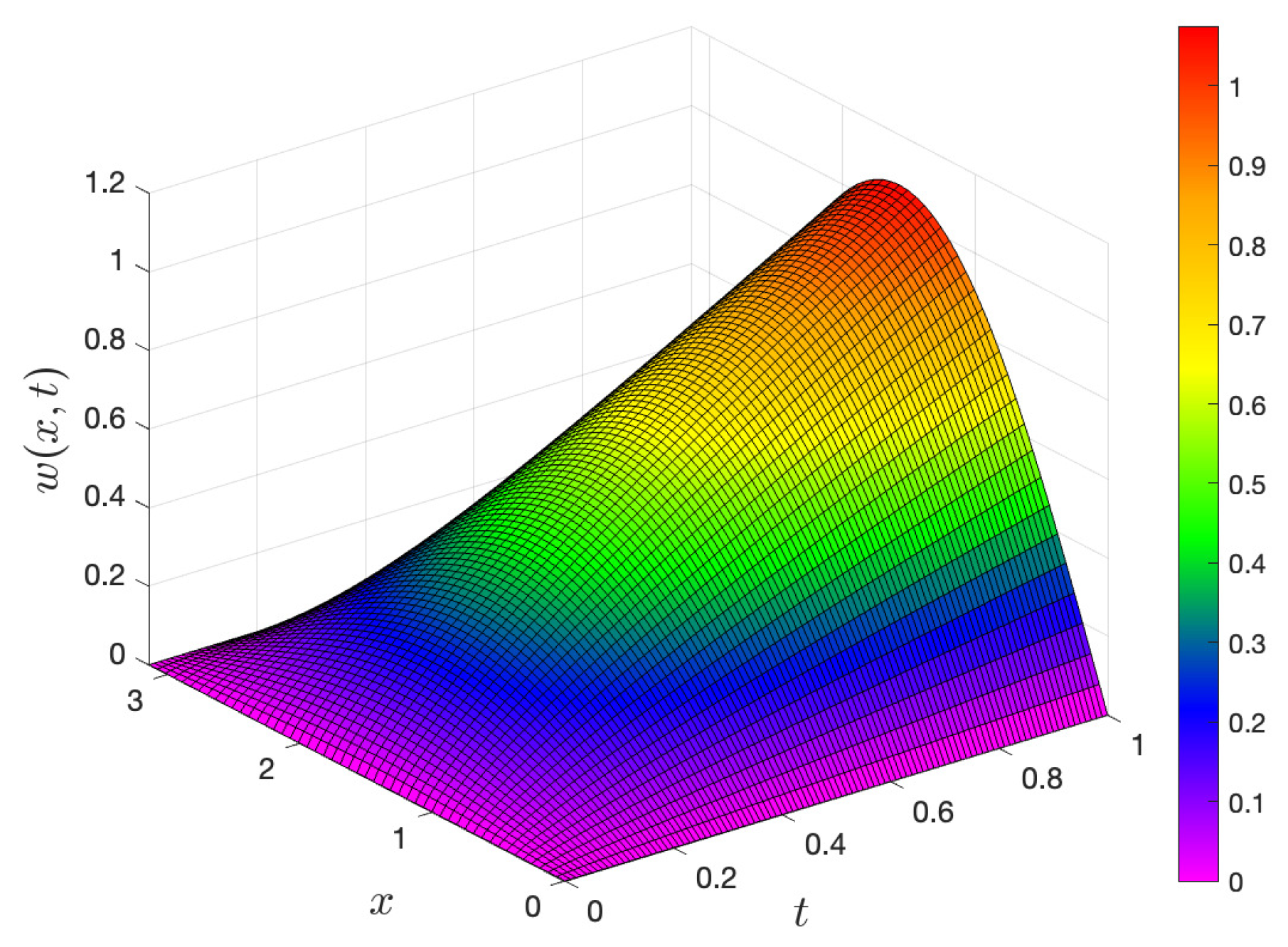
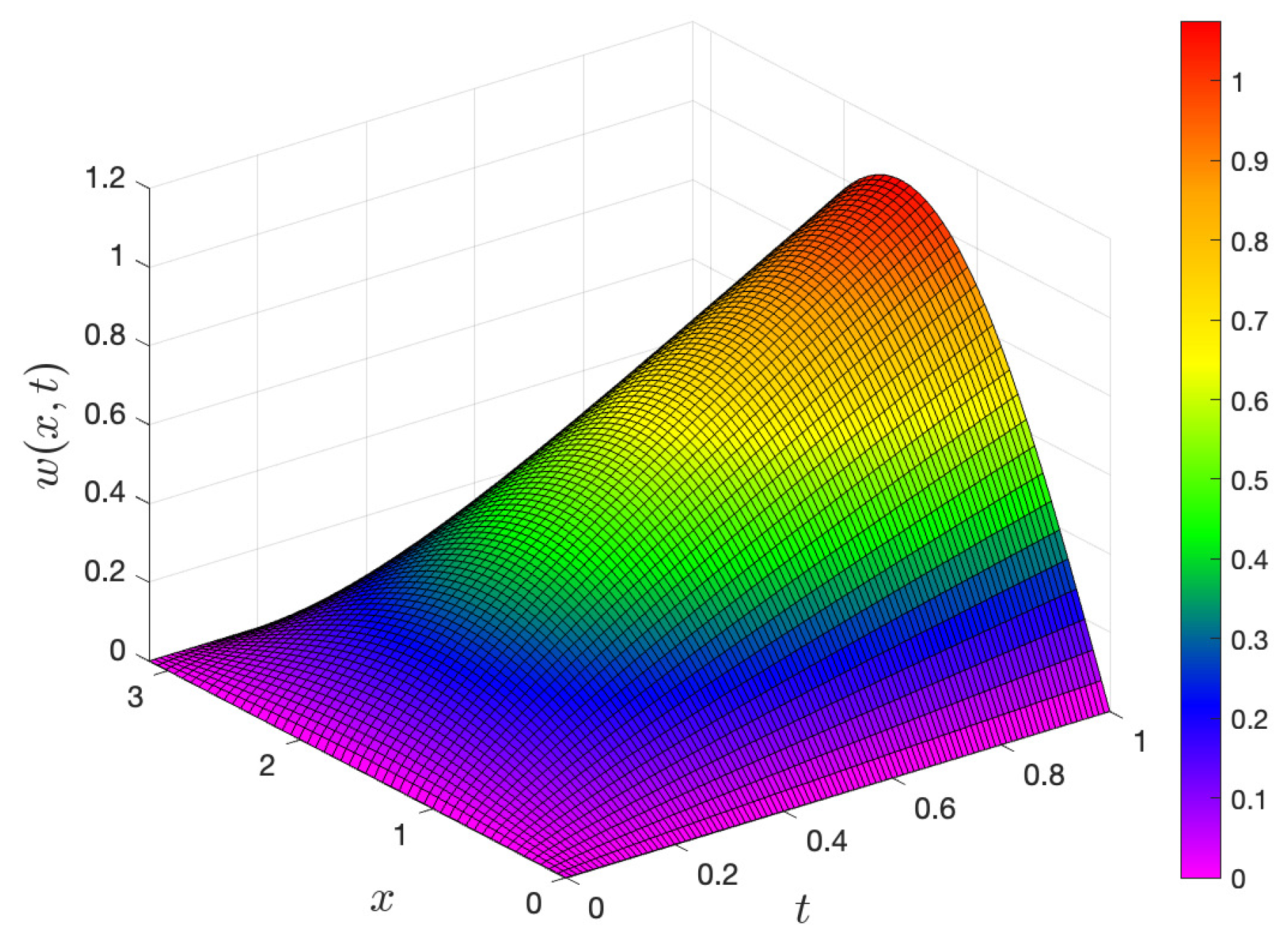
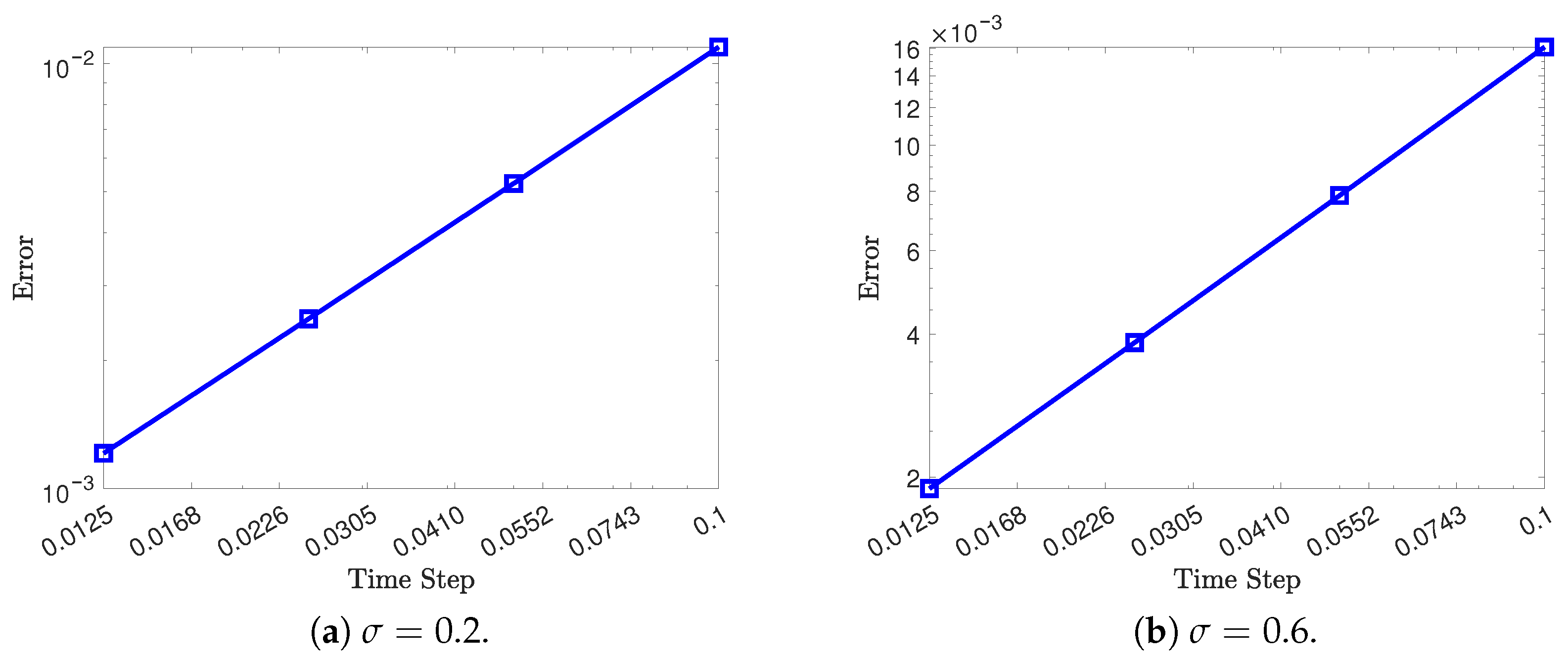
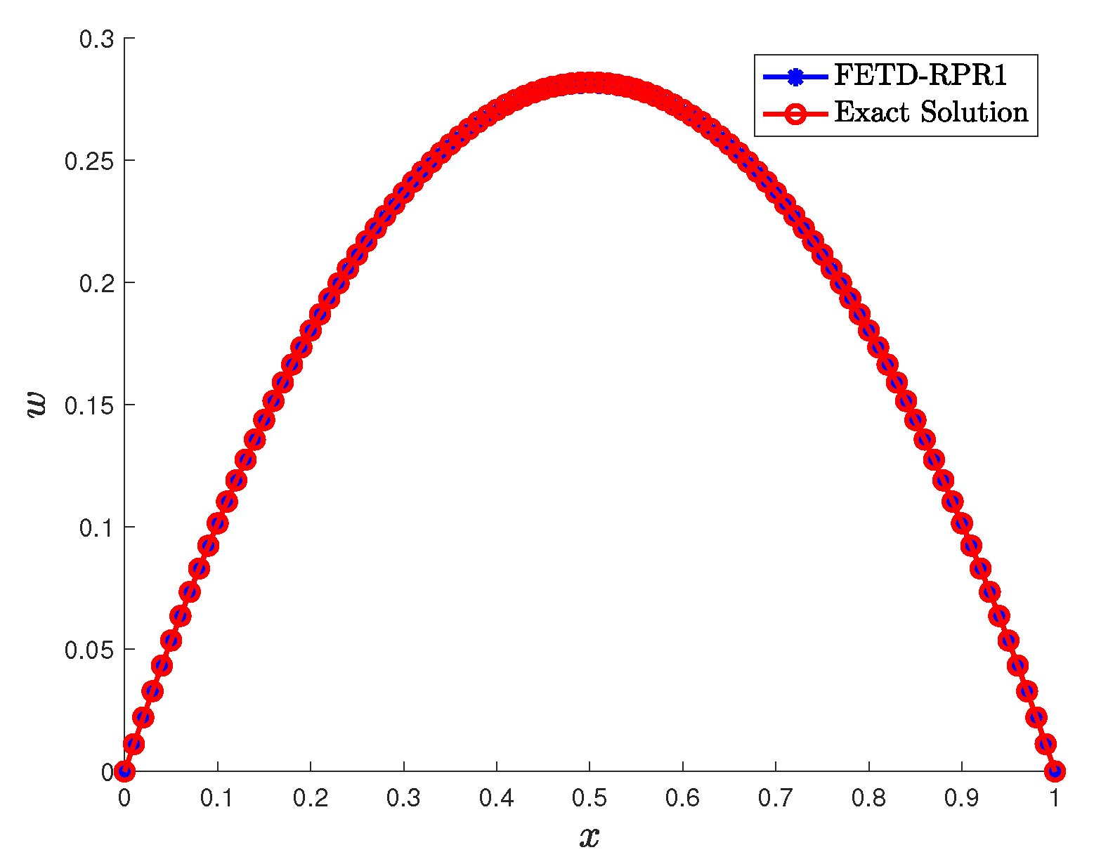
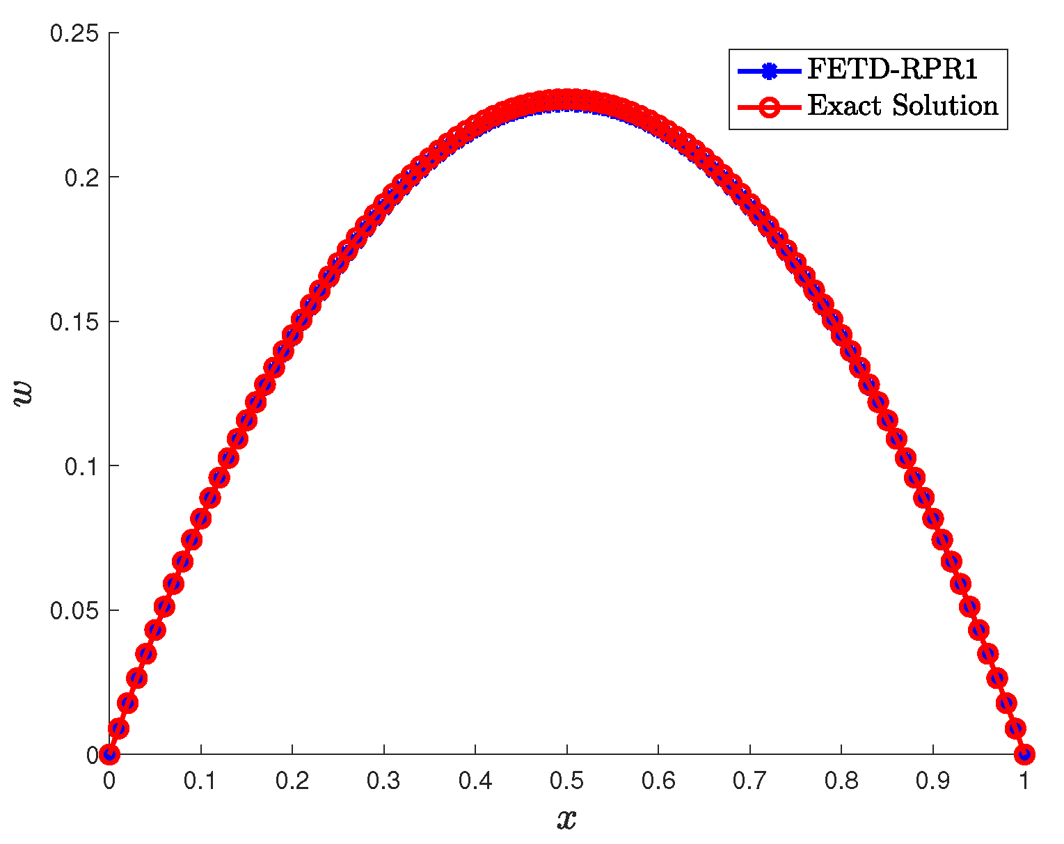
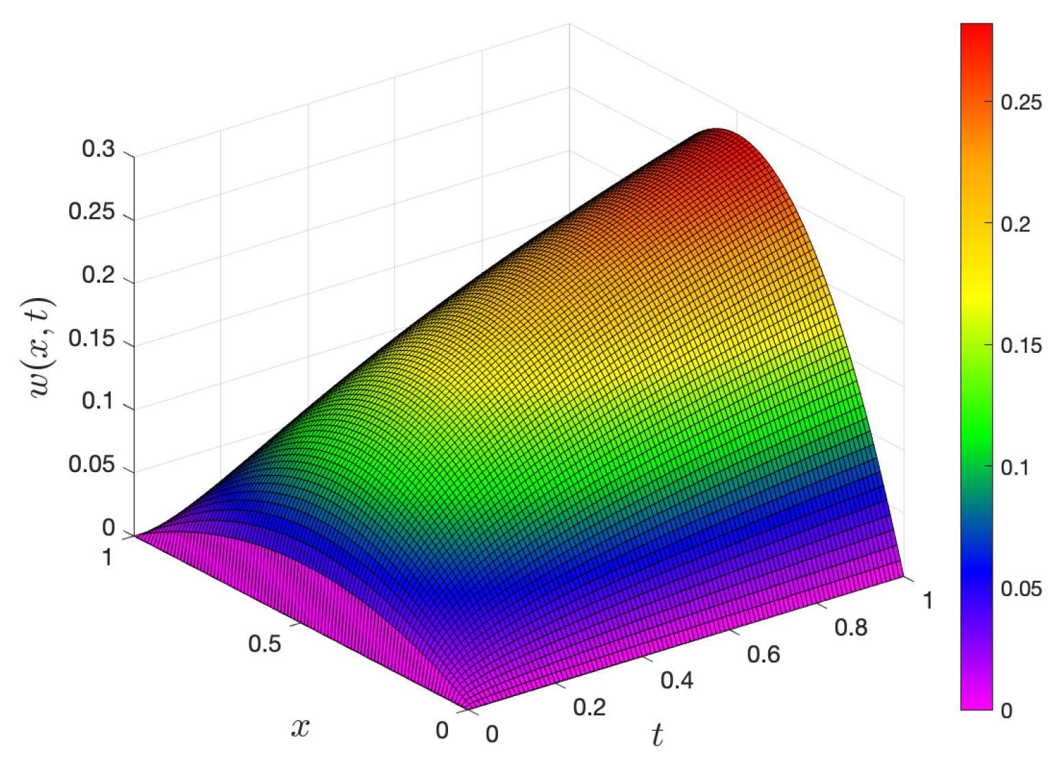
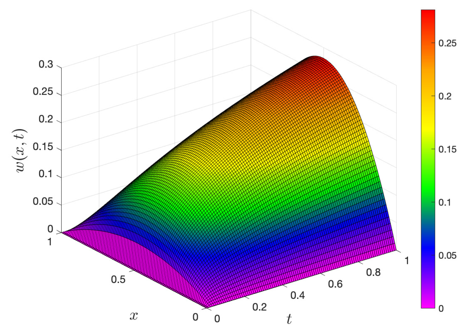
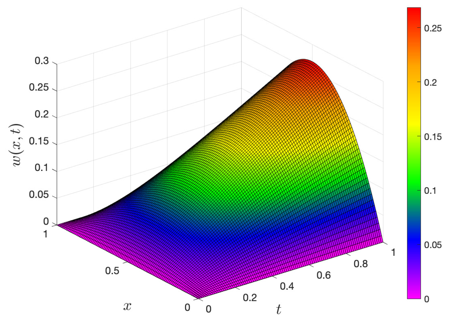
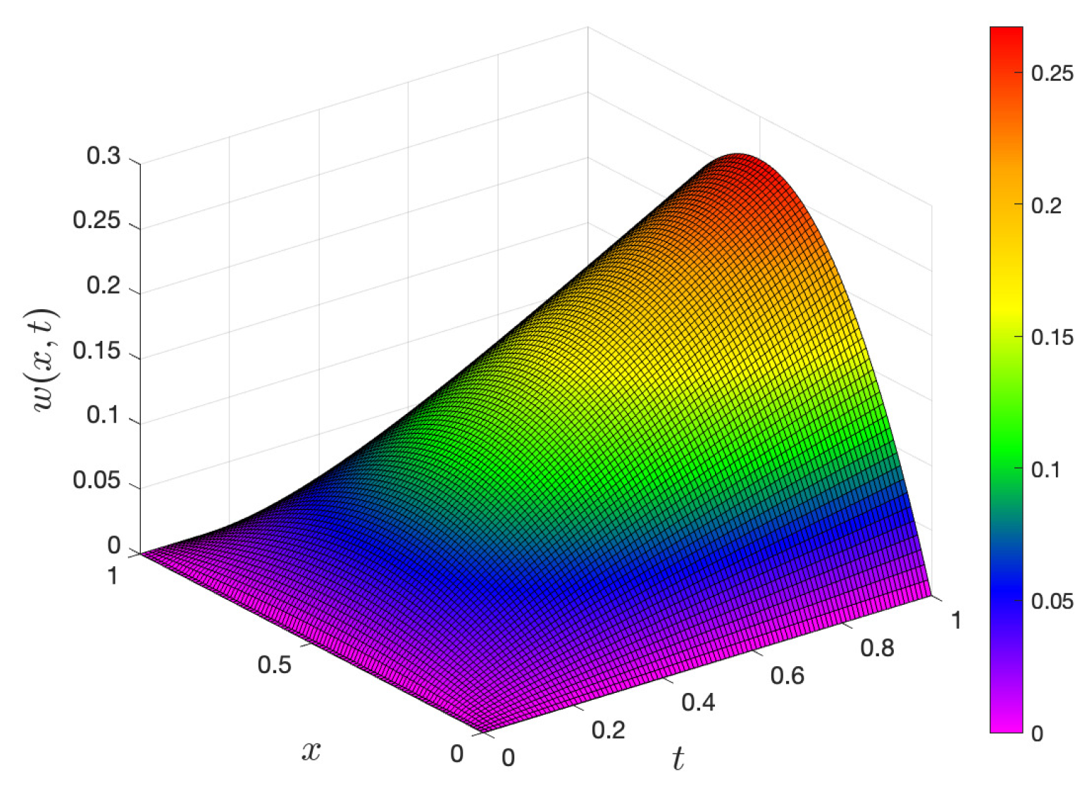
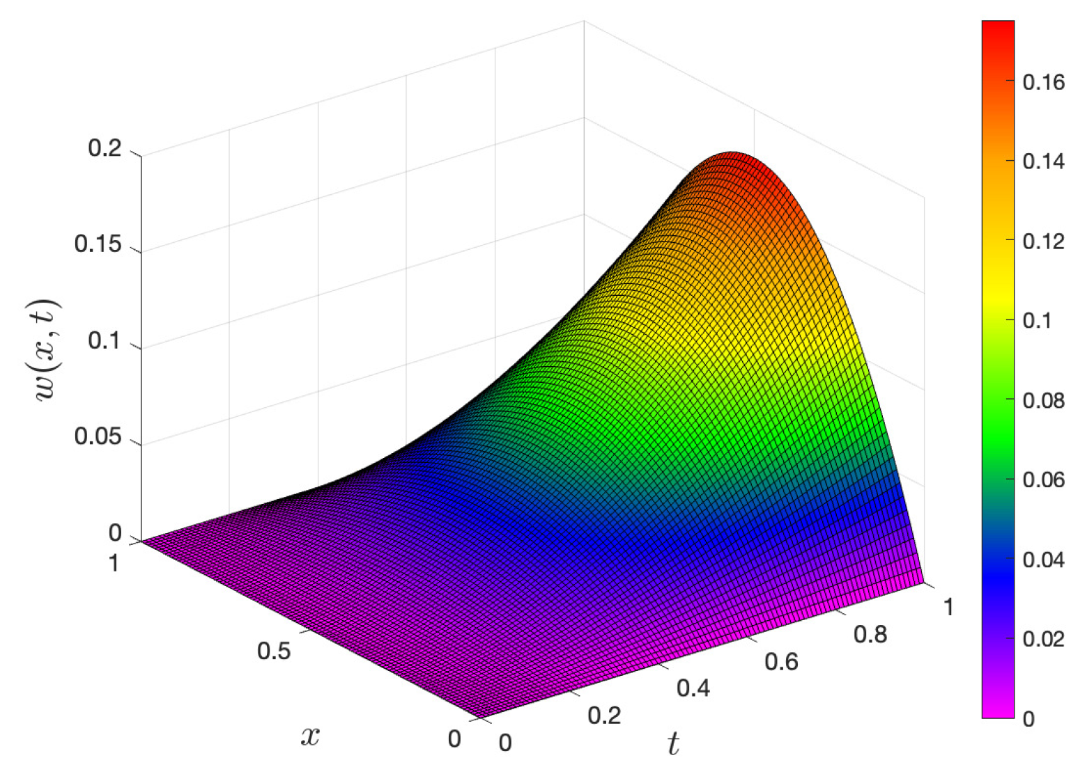
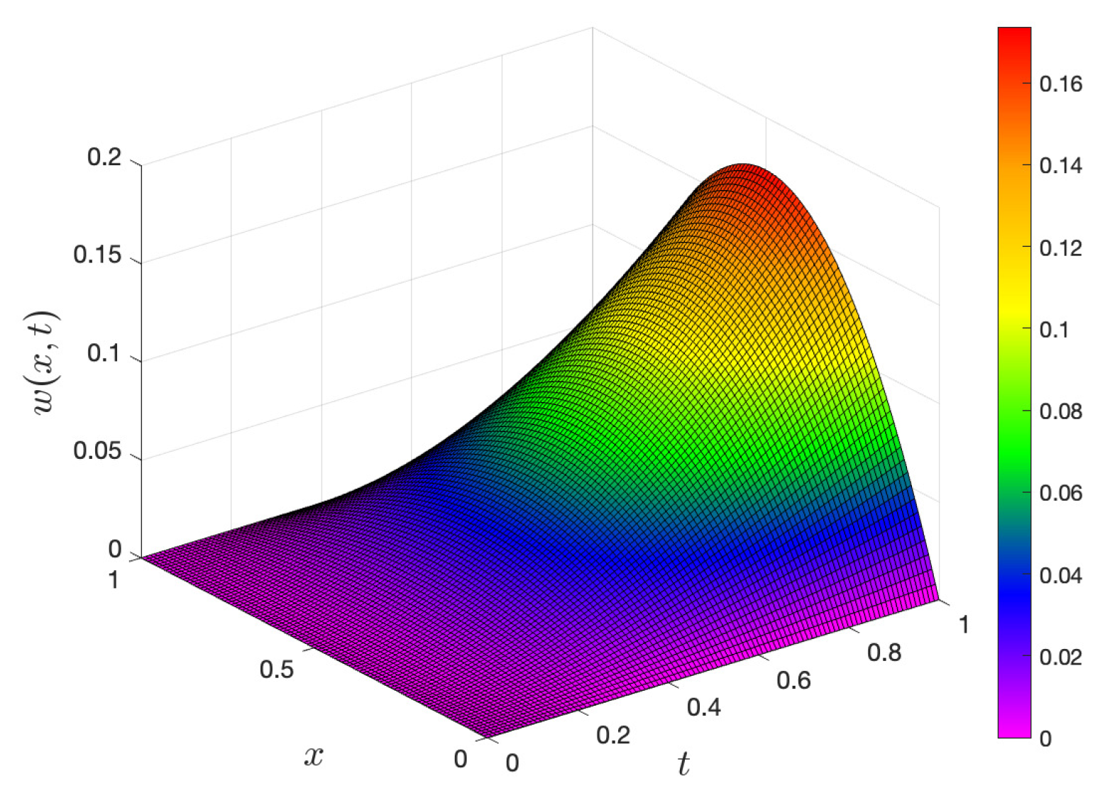
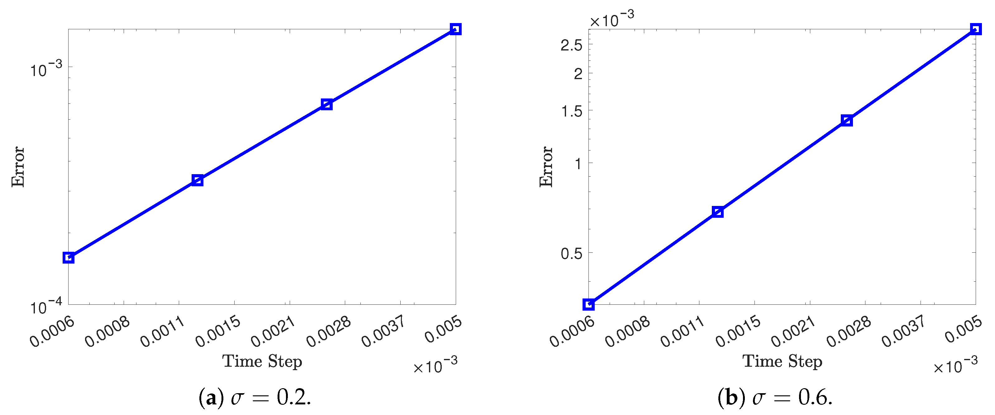
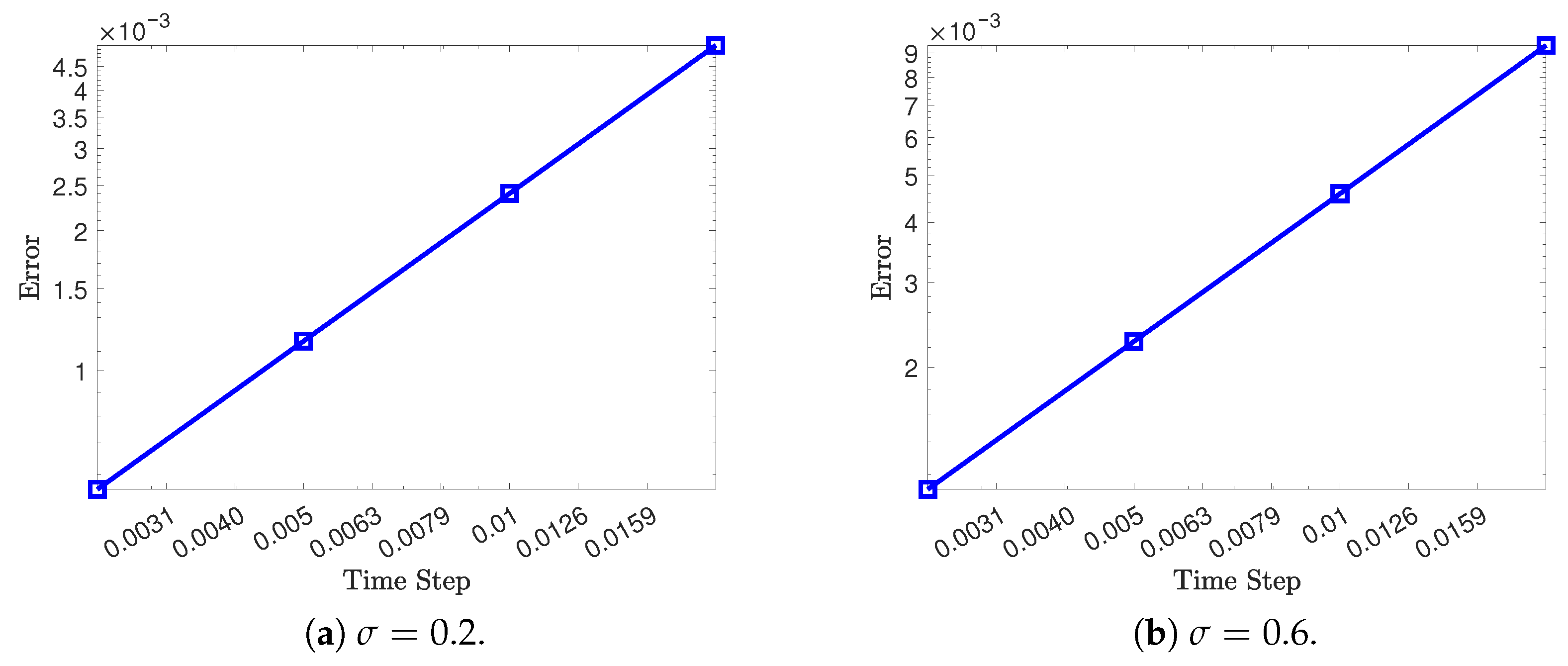
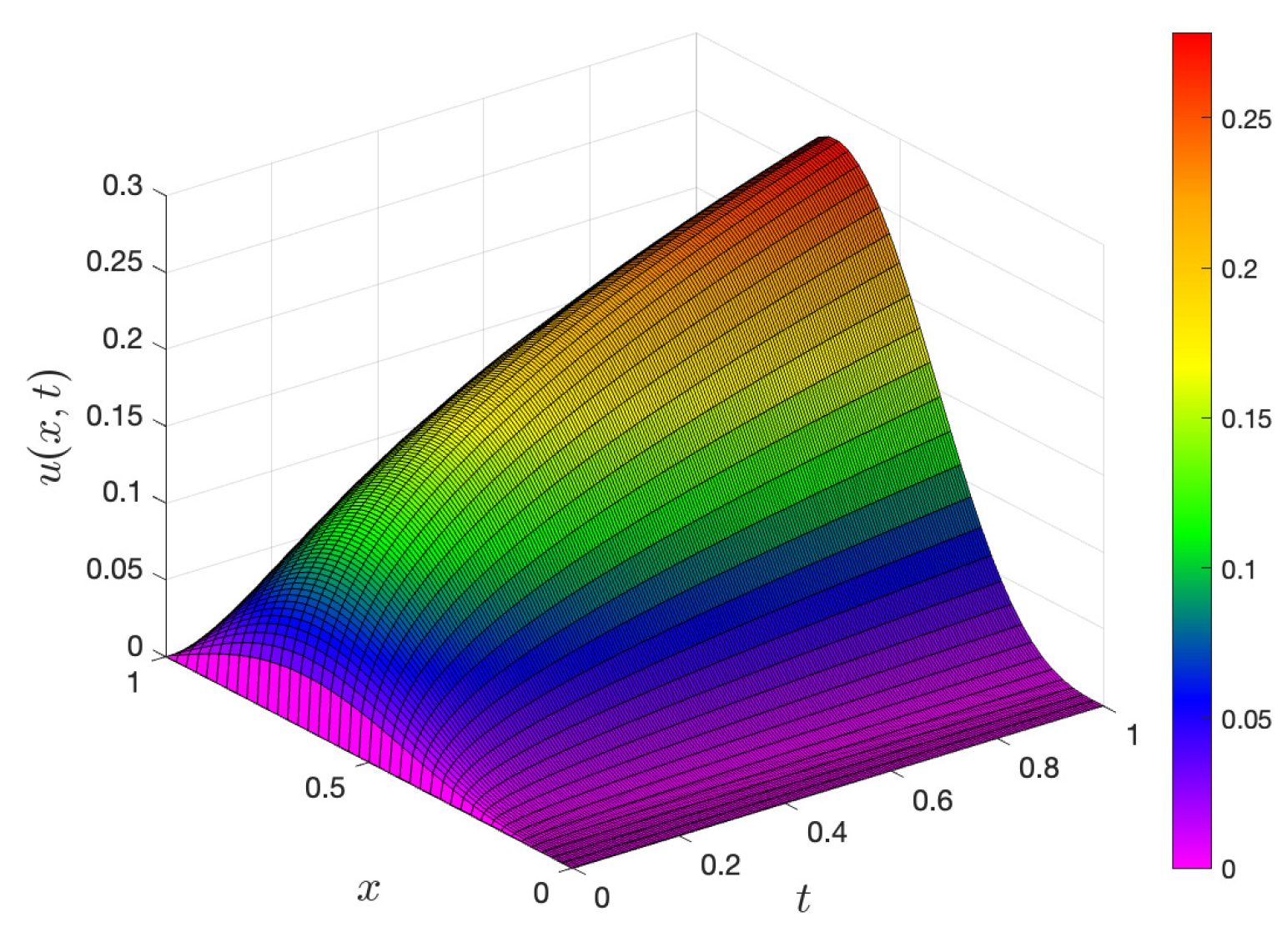
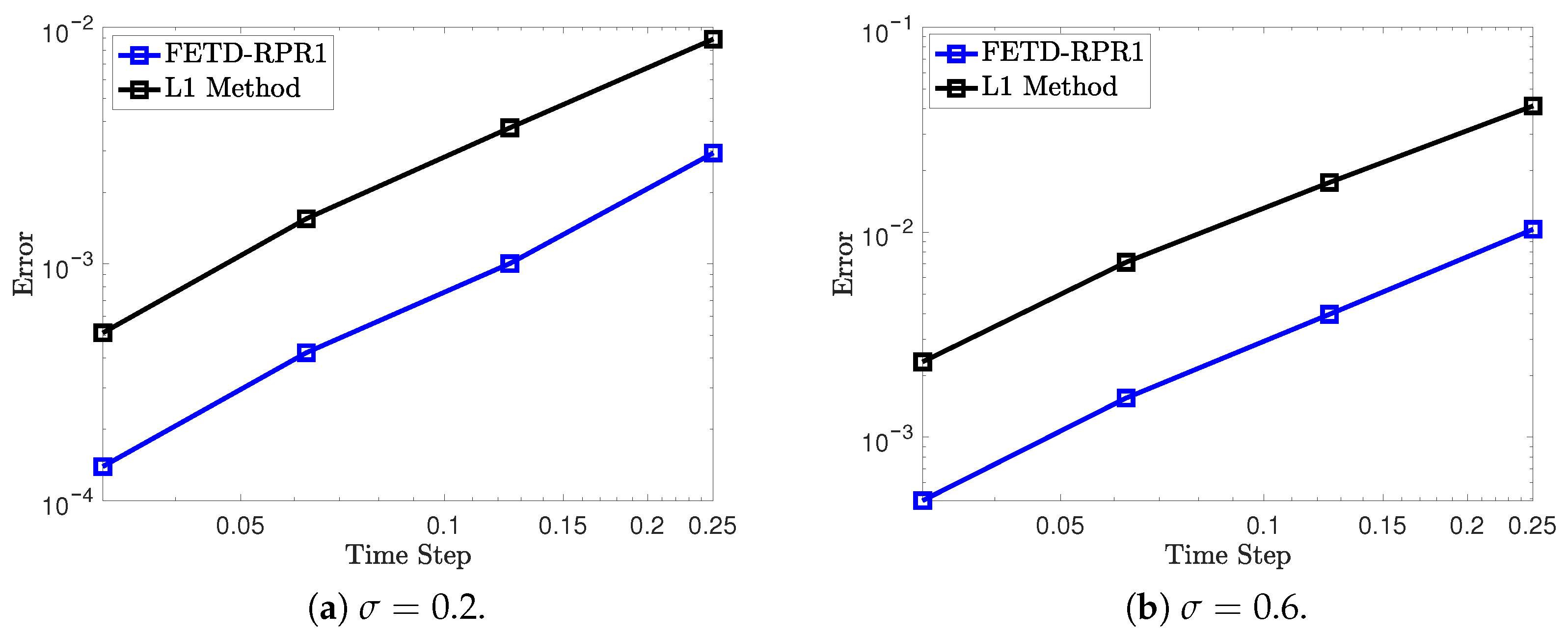
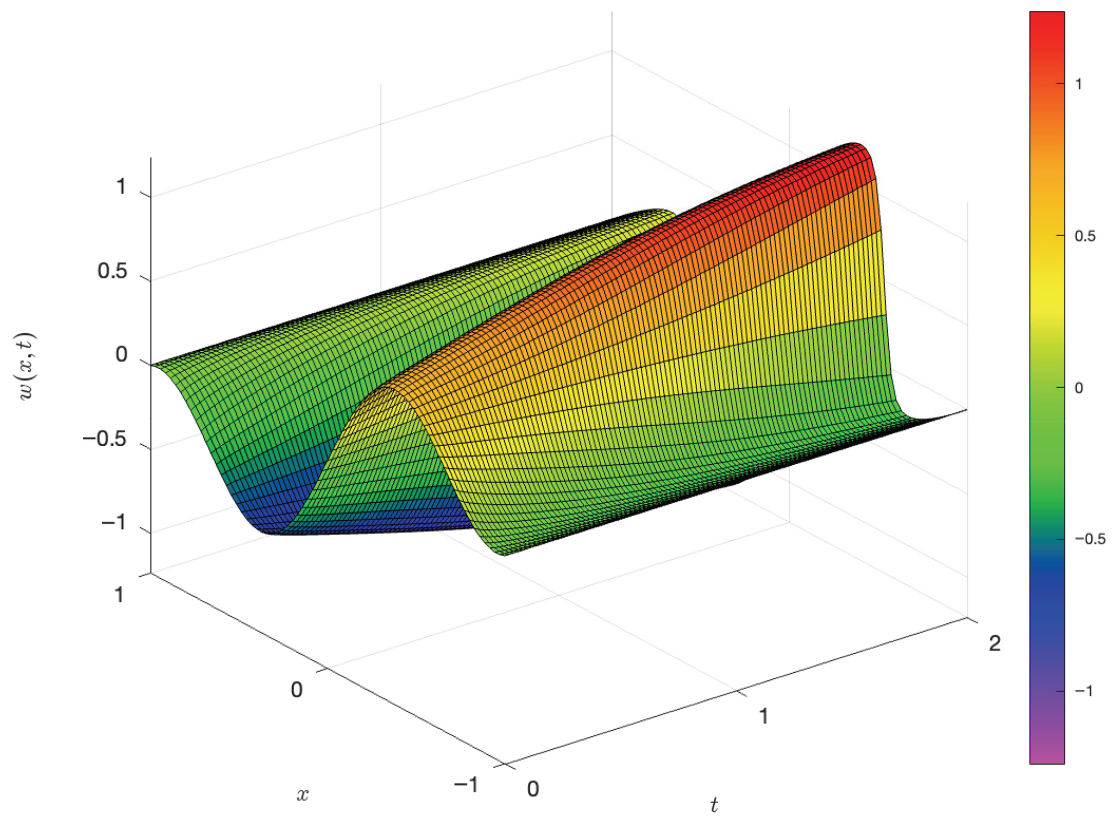
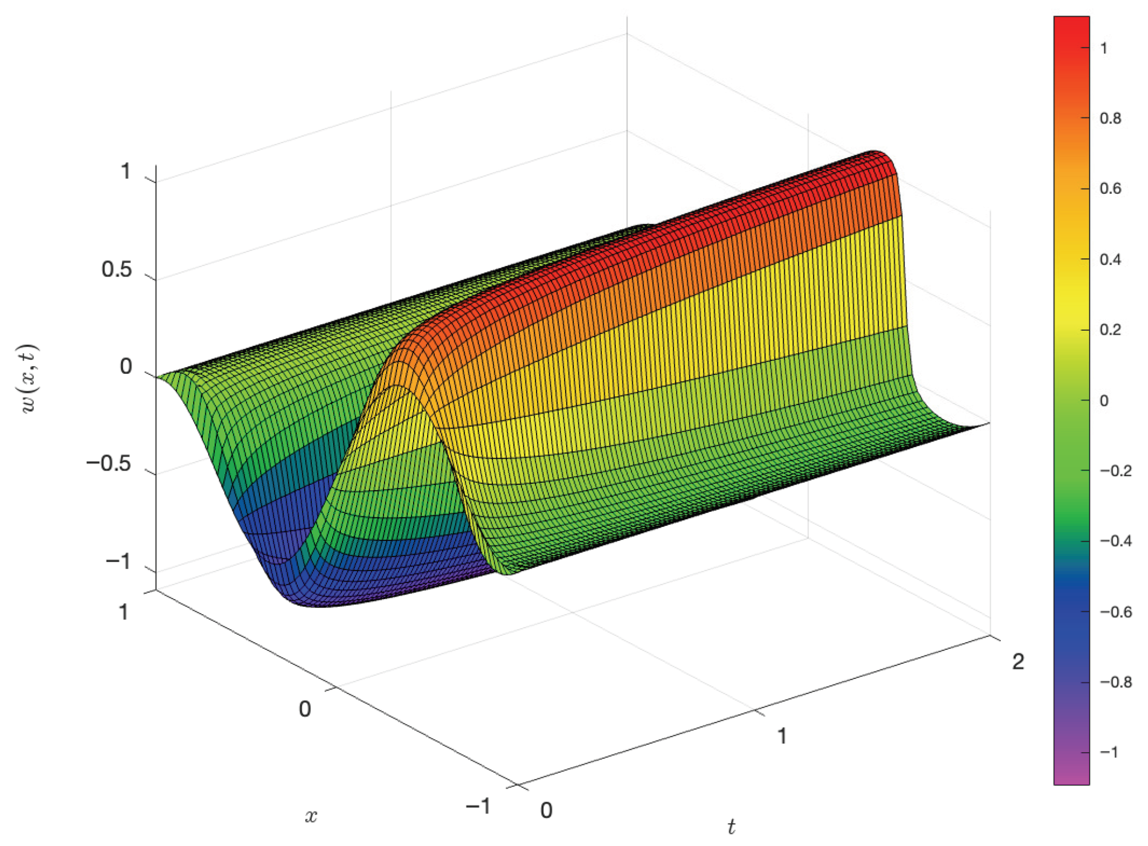
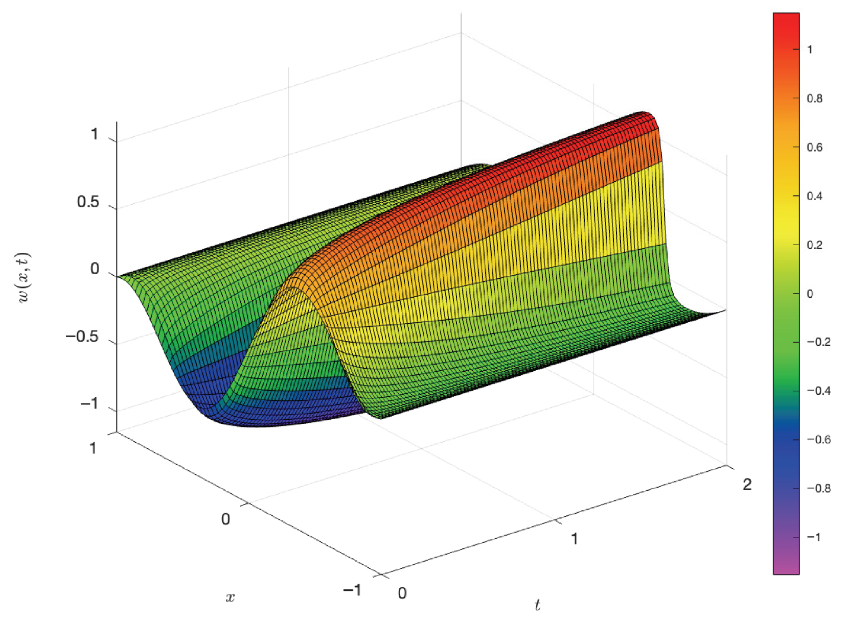
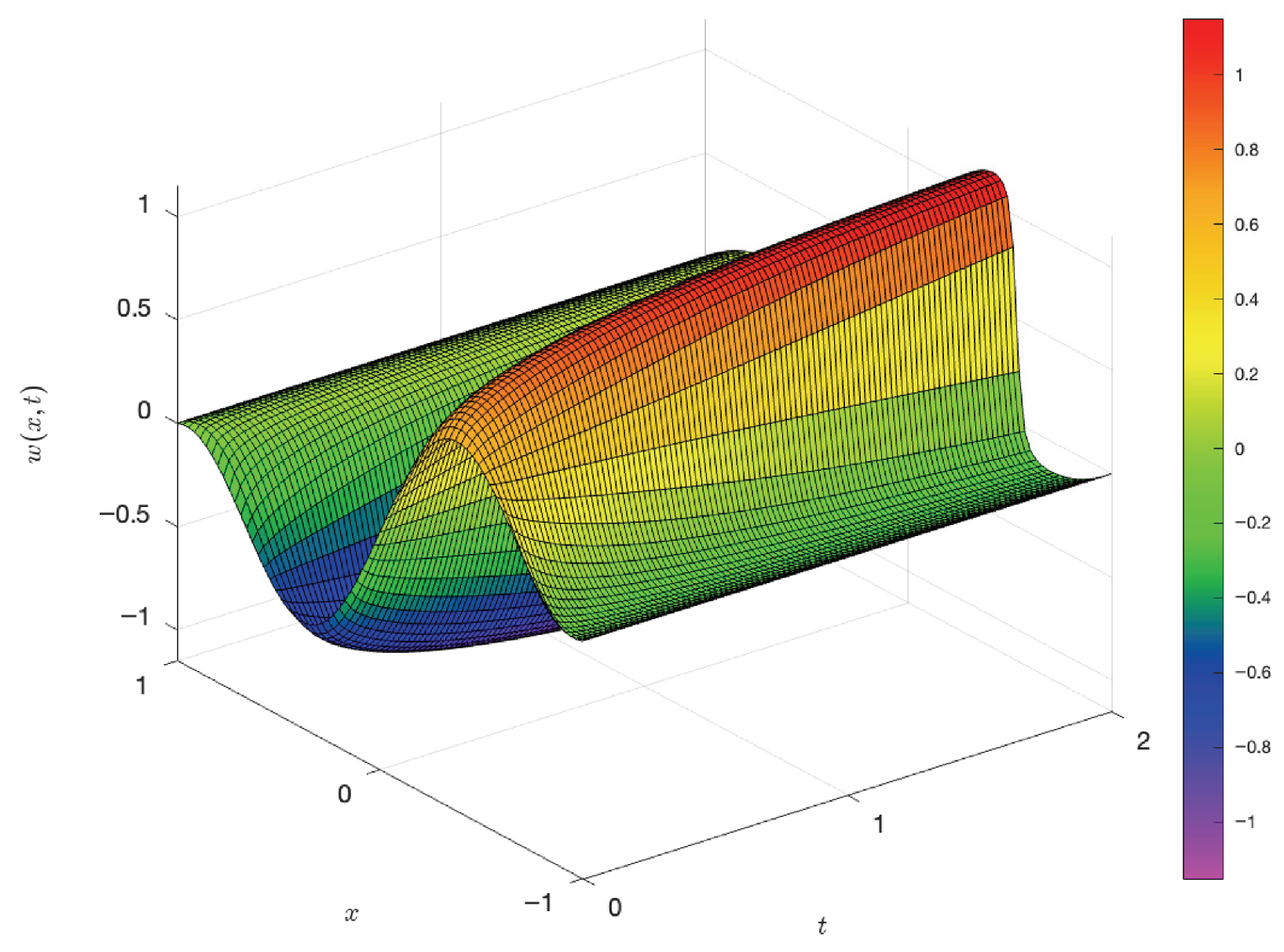
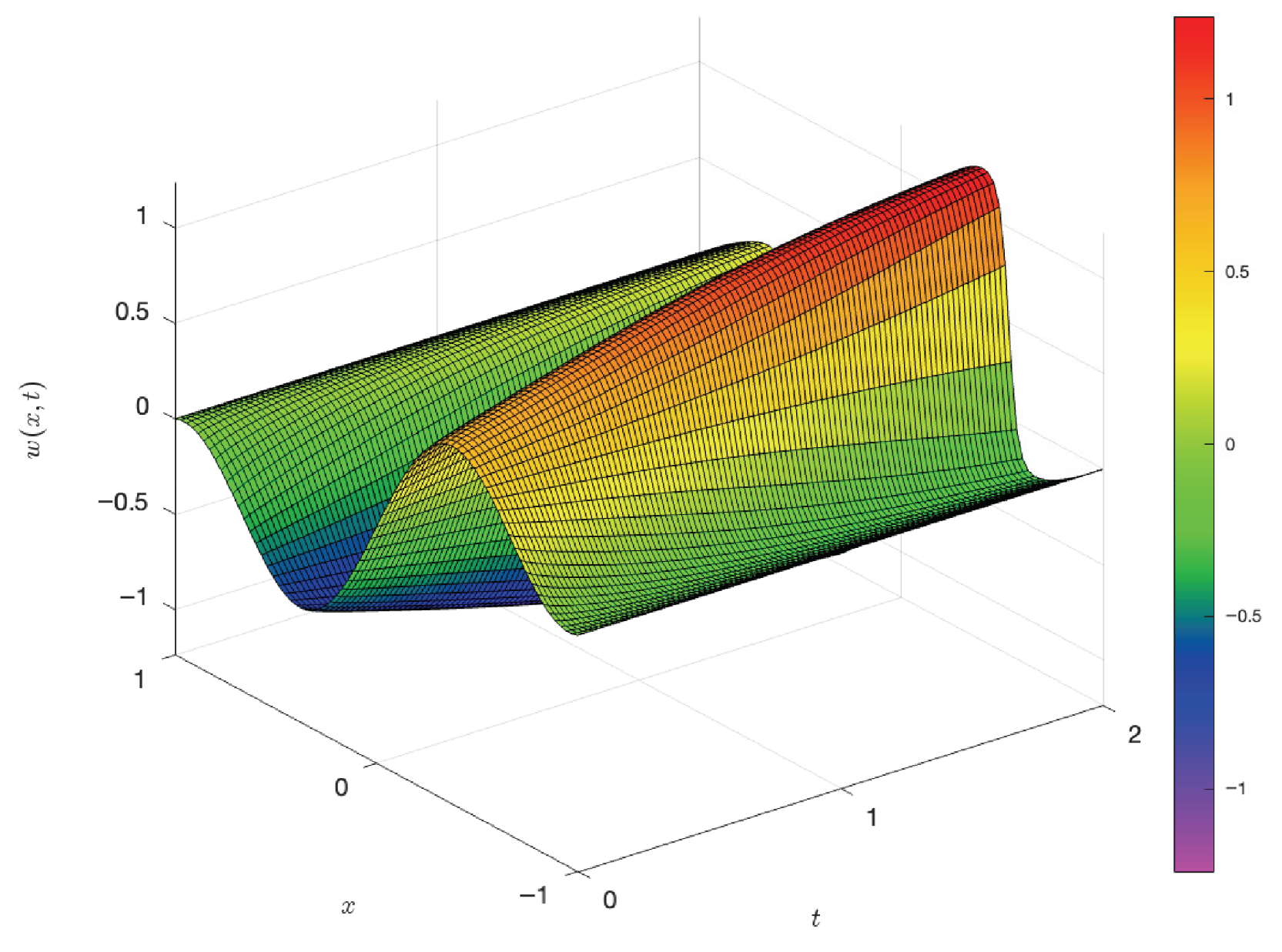
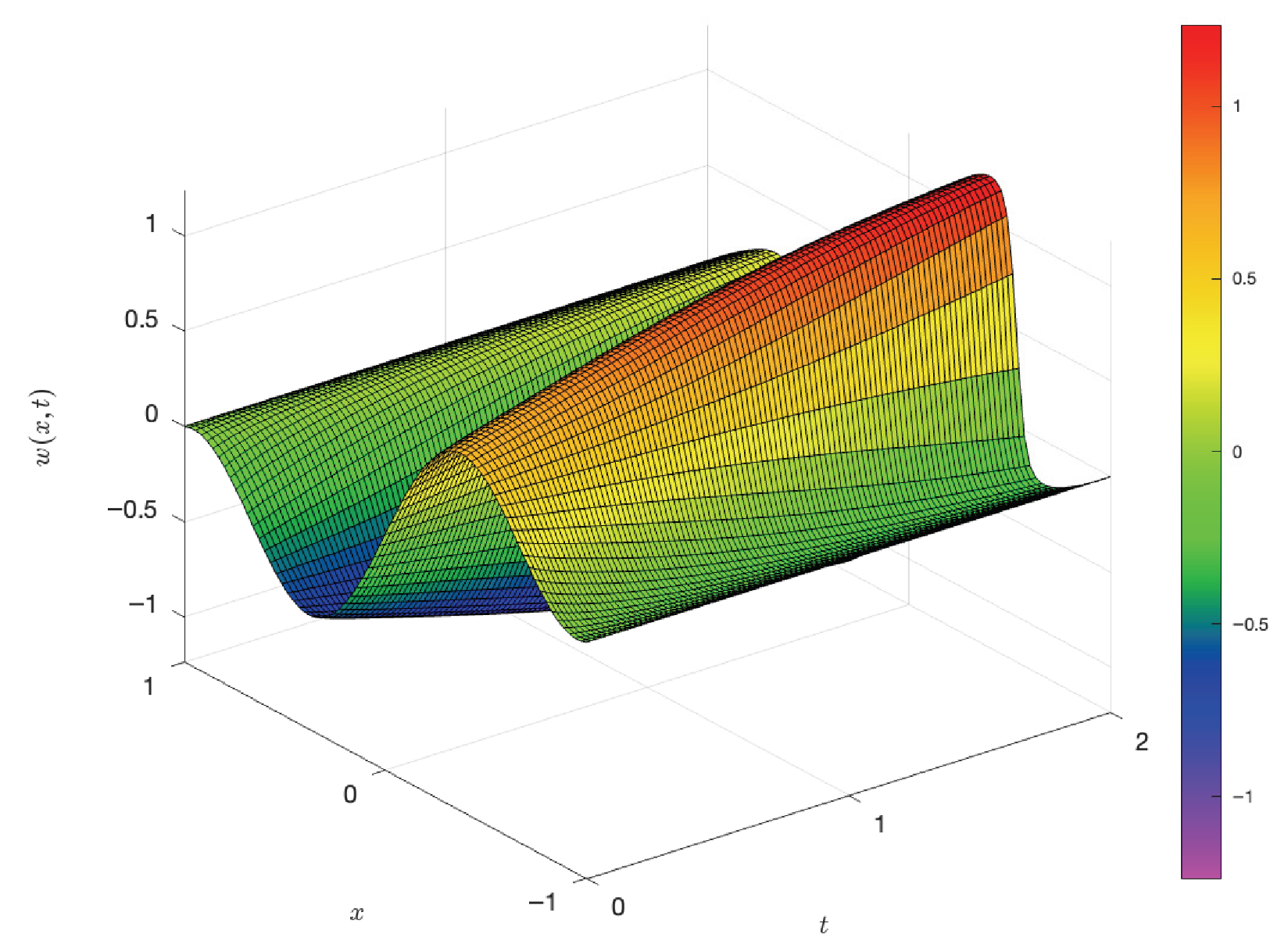
displays the numerical outcomes for Example 1, detailing the numerical errors, convergence order, and CPU time when $\epsilon =2\times {10}^{-5}$. The convergence plots in Figure 7 (also see Appendix A, Figure A1) clearly demonstrate the first-order convergence of our proposed algorithm, which is consistent with the theoretical expectations. Furthermore, Figure 8 and Figure 9 (Appendix A, Figure A2 and Figure A3) and Figure 10 and Figure 11 (Appendix A, Figure A4, Figure A5, Figure A6, Figure A7, Figure A8 and Figure A9) present the 2D and 3D matching solution plots, respectively, with parameters $k=0.05$, $T=2$, $h=0.0628$, and $\epsilon =1\times {10}^{-7}.$ It is evident from these plots that the numerical and exact solutions are in excellent agreement, indicating the high accuracy of the proposed method.

In particular, the overlap between the numerical and exact solution surfaces confirms that the error remains minimal across the computational domain. This visual agreement is further supported by the small numerical error values reported in Table 1. Additionally, the smoothness and stability of the solution profiles suggest that the method effectively handles the problem without introducing numerical oscillations or instability.

Overall, these results verify that the proposed algorithm is not only convergent but also reliable, efficient, and capable of producing highly accurate solutions even for small values of $\epsilon$. The consistency between the tabulated errors, convergence behavior, and graphical results strengthens the validity and robustness of the method for solving such problems.

Example 2.

Consider the following two-dimensional linear time-fractional reaction–diffusion equation:

$$\left\{\begin{array}{c}{}^{c}D^{\sigma }w=\kappa \left({\displaystyle \frac{{\partial }^{2}w}{\partial x^2}}+{\displaystyle \frac{{\partial }^{2}w}{\partial y^2}}\right)+2{\pi }^2\kappa w+f(x,t),t\ge 0,x,y\in [0,1]\times [0,1],\hfill \\ w(x,y,0)=\sin \left(\pi x\right)\sin \left(\pi y\right),\hfill \\ w(0,0,t)=w(1,1,t)=0,\hfill \end{array}\right.$$

where

$$f(x,t)=\sin \left(\pi x\right)\sin \left(\pi y\right){\displaystyle \frac{\mathrm{\Gamma }(\theta +1)}{\mathrm{\Gamma }(\theta -\sigma +1)}}{t}^{\theta -\sigma }.$$

In this case, the exact solution is given as follows:

$$w(x,y,t)=\left(t^{\theta }+1\right)\sin \left(\pi x\right)\sin \left(\pi y\right),\theta >\sigma .$$

In

Table 2. Numerical results for Example 2.

$\mathit{\sigma }$	k	h	Error	OC	CPU Time
0.2	0.1000	0.047619	$2.2618\times {10}^{-2}$	-	$2.3000\times {10}^{-2}$
	0.0500	0.047619	$1.0867\times {10}^{-2}$	1.06	$8.0550\times {10}^{-2}$
	0.0250	0.047619	$5.2813\times {10}^{-3}$	1.04	$2.9221\times {10}^{-1}$
	0.0125	0.047619	$2.5816\times {10}^{-3}$	$1.03$	$1.1377$
0.4	0.1000	0.047619	$4.0636\times {10}^{-2}$	-	$2.2280\times {10}^{-2}$
	0.0500	0.047619	$1.9668\times {10}^{-2}$	1.05	$8.0030\times {10}^{-3}$
	0.0250	0.047619	$1.4027\times {10}^{-3}$	1.03	$3.0106\times {10}^{-3}$
	0.0125	0.047619	$4.7095\times {10}^{-3}$	$1.03$	$1.1311$
0.6	0.1000	0.047619	$5.8776\times {10}^{-2}$	-	$2.3240\times {10}^{-2}$
	0.0500	0.047619	$2.8630\times {10}^{-2}$	1.04	$8.1870\times {10}^{-2}$
	0.0250	0.047619	$1.4027\times {10}^{-2}$	1.03	$3.0404\times {10}^{-1}$
	0.0125	0.047619	$6.8932\times {10}^{-3}$	1.03	$1.1286$
0.8	0.1000	0.047619	$7.6813\times {10}^{-2}$	-	$3.7300\times {10}^{-2}$
	0.0500	0.047619	$3.7628\times {10}^{-2}$	1.03	$8.3800\times {10}^{-2}$
	0.0250	0.047619	$1.8488\times {10}^{-3}$	1.03	$3.0343\times {10}^{-2}$
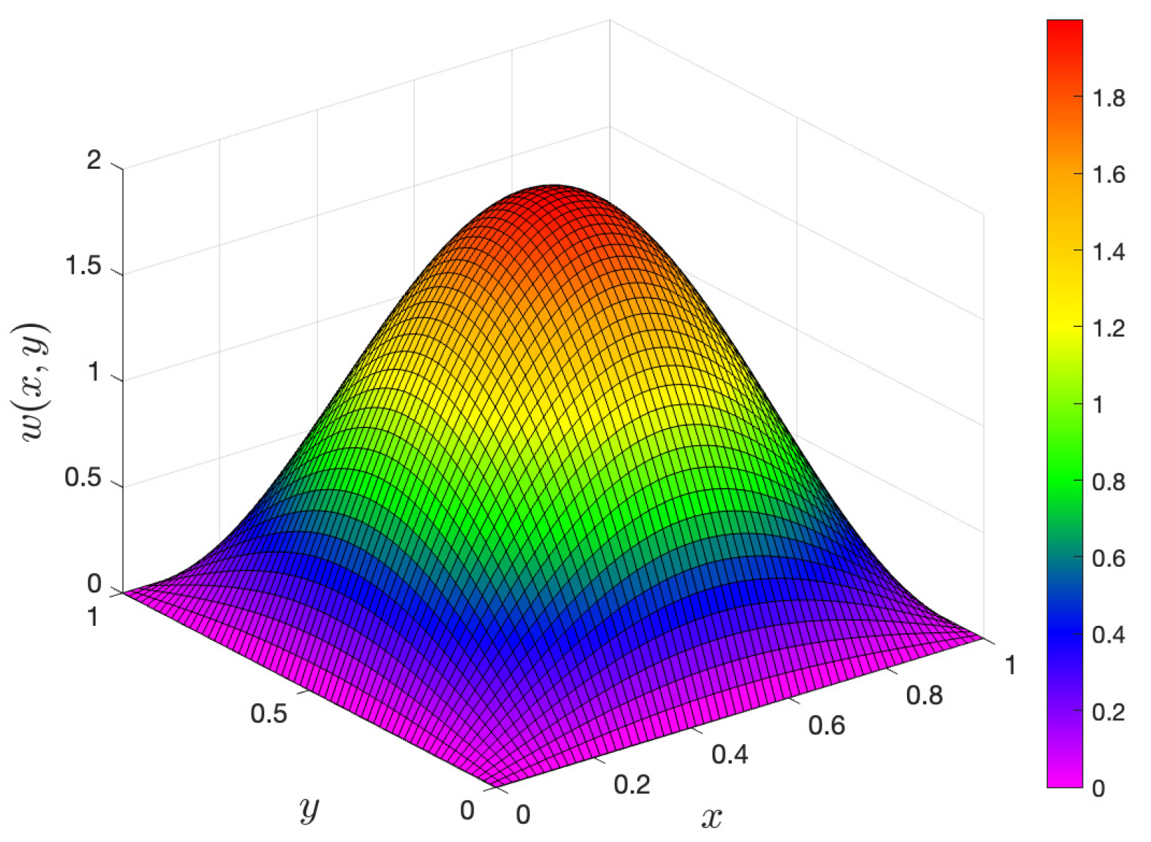
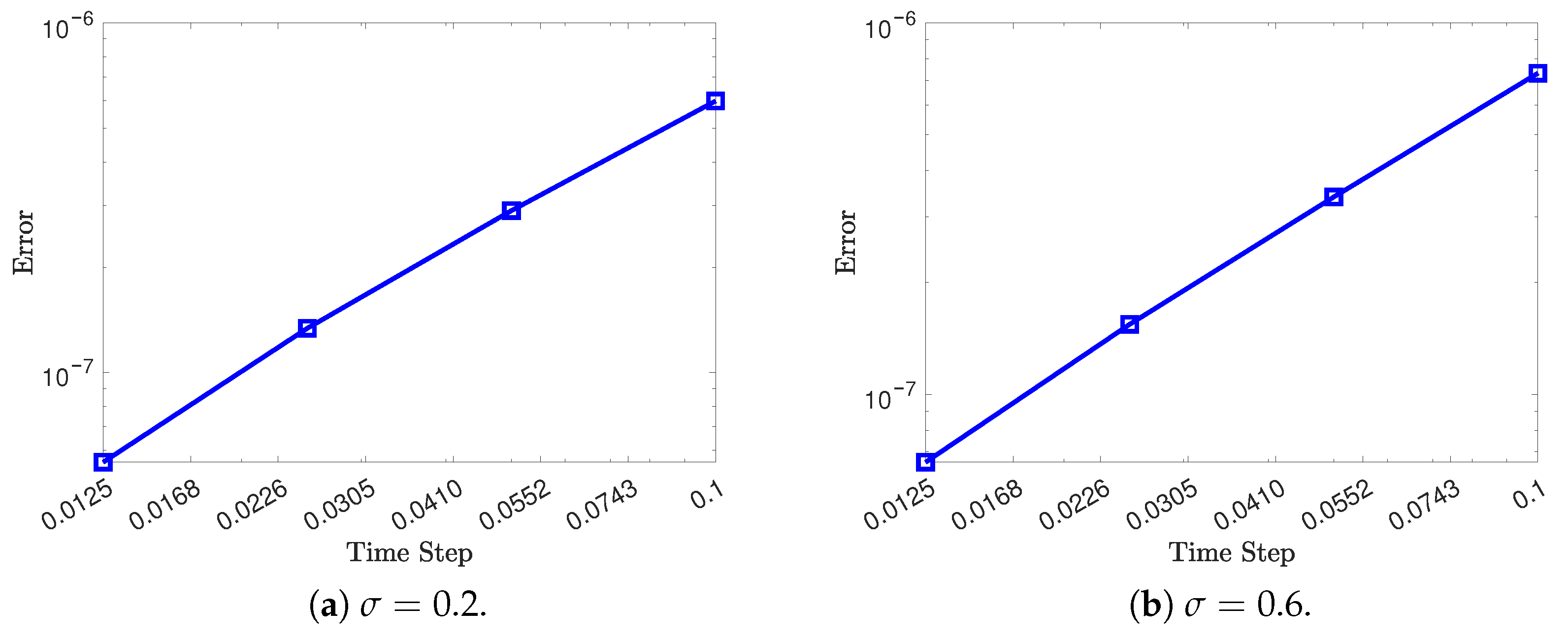
	0.0125	0.047619	$9.0975\times {10}^{-3}$	1.02	$1.1345$

, the numerical errors, convergence order, and CPU time for the 2D linear Example 2 are presented for the FETD-RPR1 scheme under successive grid refinement. The results clearly indicate a consistent reduction in error as the mesh is refined, demonstrating the stability and accuracy of the proposed method. The computed convergence order, as illustrated in Figure 12 (Appendix A, Figure A10) for the parameters $\kappa =5\times {10}^{-6}$ and $\theta =\sigma +0.05$, confirms that the scheme achieves the expected first-order convergence rate.

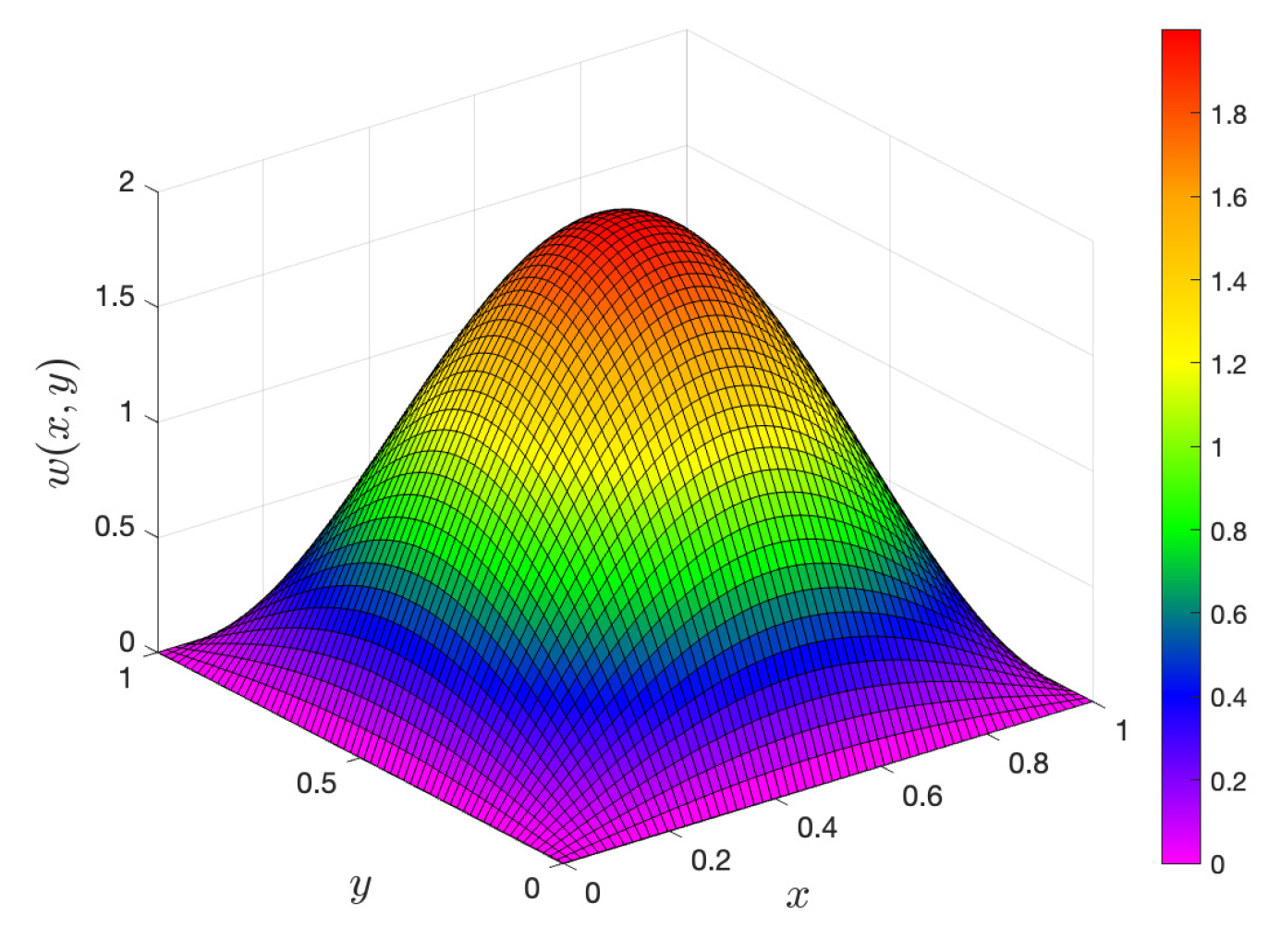
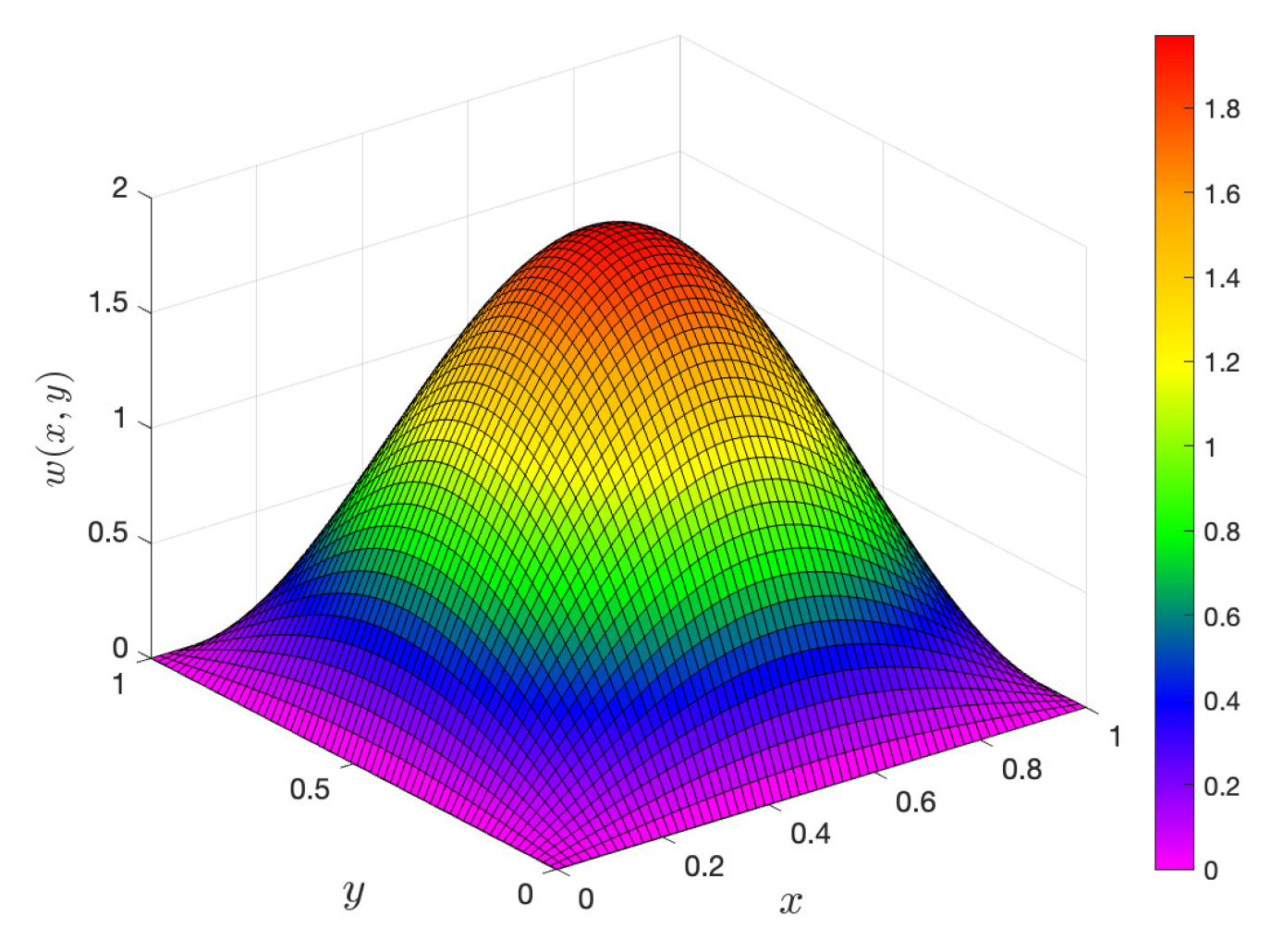
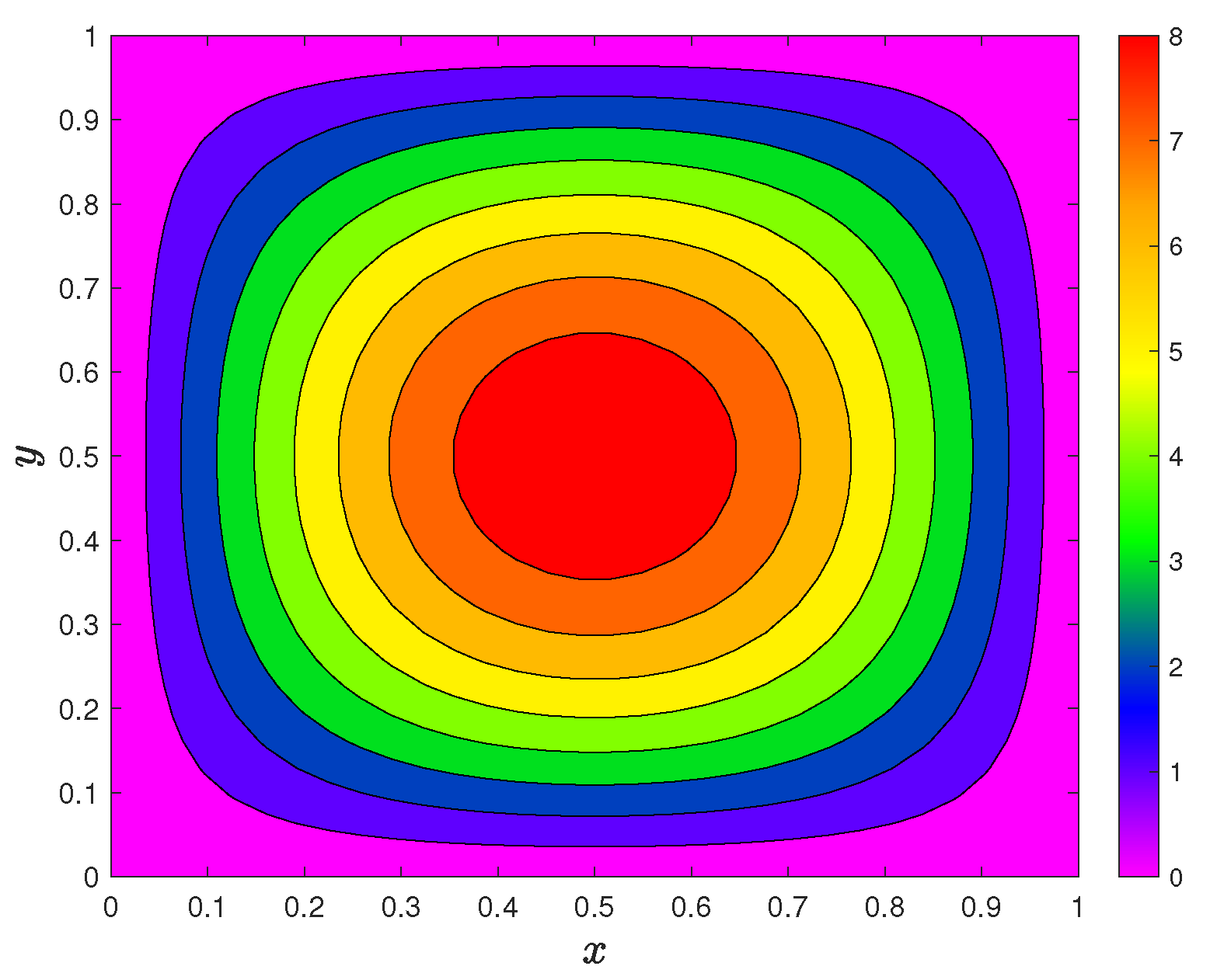
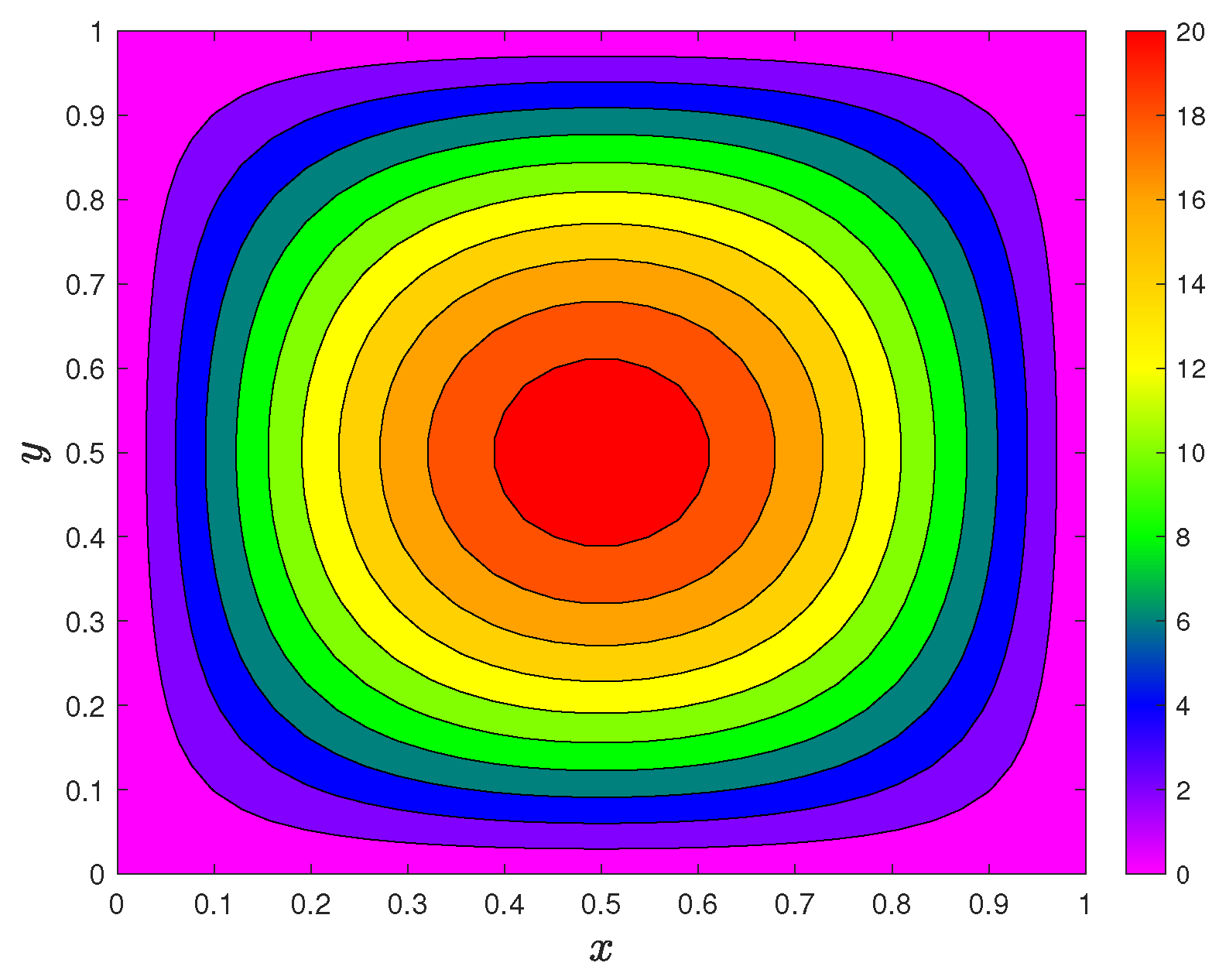
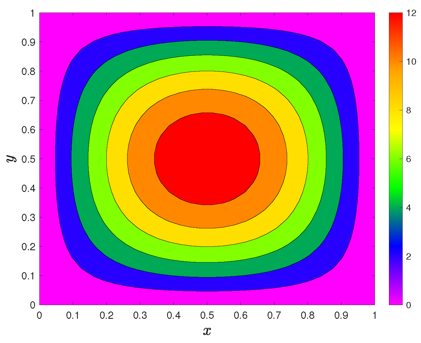
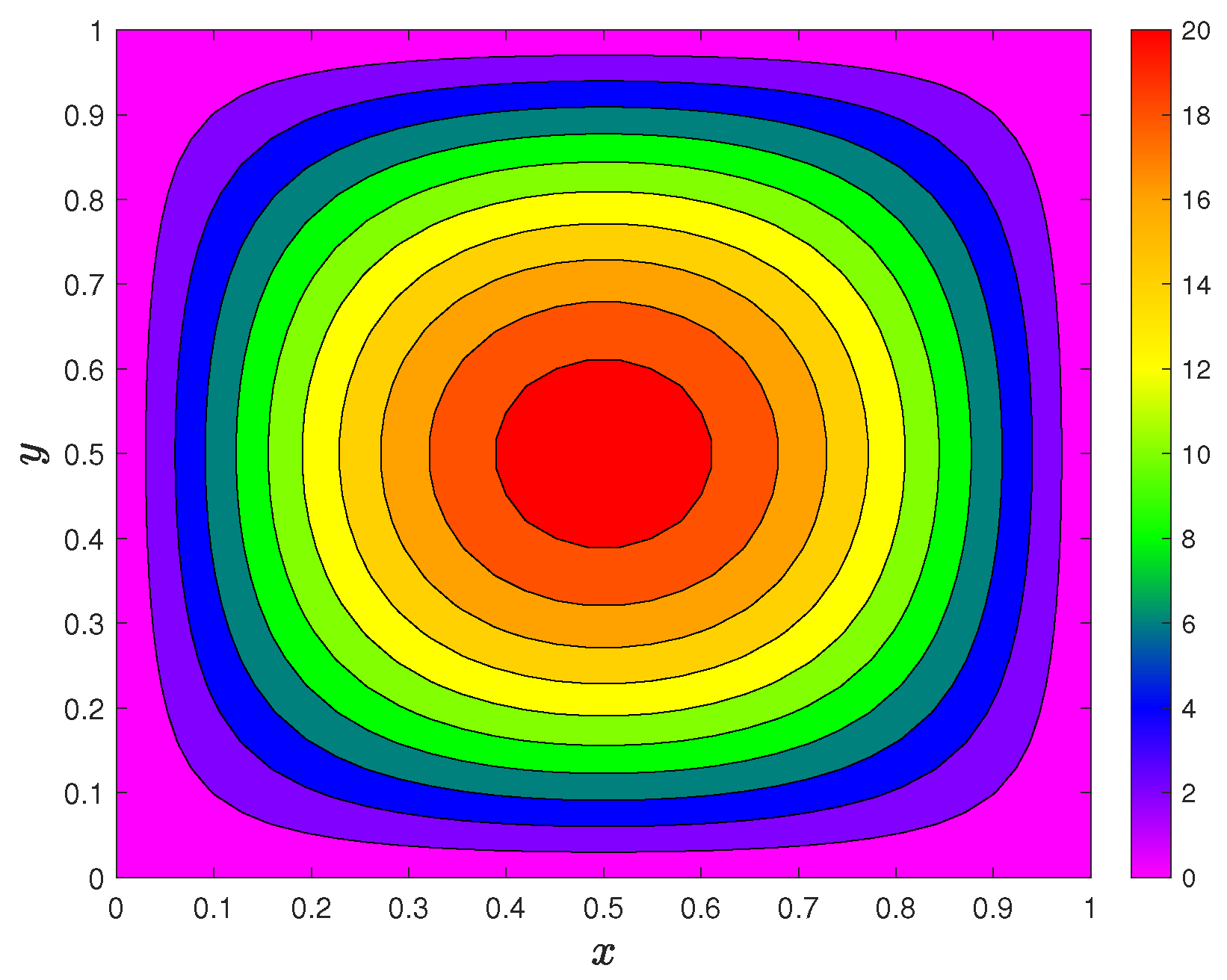
Figure 13 and Figure 14 (Appendix A, Figure A11, Figure A12, Figure A13, Figure A14, Figure A15 and Figure A16) display the 3D numerical solution surfaces alongside the corresponding exact solutions, while the contour plots in Figure 15 and Figure 16 (Appendix A, Figure A17 and Figure A18) provide further insight into the spatial behavior of the solution for $\kappa =5\times {10}^{-3}$ and $\theta =\sigma +0.5$. From these visualizations, it is evident that the numerical solutions closely match the exact solutions across the entire computational domain. The near-perfect overlap of contours and the absence of visible distortions or oscillations further suggest that the numerical errors are minimal and uniformly distributed.

Moreover, the smoothness of the solution surfaces and the consistency of contour levels highlight the robustness of the method. These observations, together with the quantitative results reported in Table 2, confirm that the FETD-RPR1 scheme is efficient, stable, and capable of producing accurate approximations for 2D linear problems.

Example 3.

Consider the following nonlinear time-fractional reaction–diffusion equation:

$$\left\{\begin{array}{c}{}^{c}D^{\sigma }w=\epsilon {\displaystyle \frac{{\partial }^{2}w}{\partial x^2}}+w(1-w)+g(x,t),t\ge 0,x\in [0,\pi ],\hfill \\ w(x,0)=0,\hfill \\ w(0,t)=w(\pi ,t)=0,\hfill \end{array}\right.$$

where

$$g(x,t)=\sin \left(x\right)-(1-\epsilon ){\displaystyle \frac{t^{\sigma }\sin \left(x\right)}{\mathrm{\Gamma }(1+\sigma )}}+{\displaystyle \frac{t^{2\sigma }{\sin }^2\left(x\right)}{\mathrm{\Gamma }{(1+\sigma )}^2}},$$

with the exact solution

$$u(x,t)=sinx{\displaystyle \frac{t^{\sigma }}{\mathrm{\Gamma }(1+\sigma )}}.$$

Choosing $\epsilon =2\times {10}^{-5}$, we observe significantly reduced numerical errors along with lower CPU time for Example 3, as reported in

Table 3. Numerical results for Example 3.

$\mathit{\sigma }$	k	h	Error	OC	CPU Time
0.2	0.1000	0.14960	$5.9780\times {10}^{-7}$	-	$3.400\times {10}^{-3}$
	0.0500	0.14960	$2.9048\times {10}^{-7}$	1.04	$5.210\times {10}^{-3}$
	0.0250	0.14960	$1.3389\times {10}^{-7}$	1.12	$7.580\times {10}^{-3}$
	0.0125	0.14960	$5.5441\times {10}^{-8}$	$1.27$	$2.793\times {10}^{-2}$
0.4	0.1000	0.14960	$6.6856\times {10}^{-7}$	-	$3.290\times {10}^{-3}$
	0.0500	0.14960	$3.1284\times {10}^{-7}$	1.04	$5.670\times {10}^{-3}$
	0.0250	0.14960	$1.4090\times {10}^{-7}$	1.15	$8.250\times {10}^{-3}$
	0.0125	0.14960	$5.7999\times {10}^{-8}$	$1.28$	$2.972\times {10}^{-2}$
0.6	0.1000	0.14960	$7.3213\times {10}^{-7}$	-	$2.980\times {10}^{-3}$
	0.0500	0.14960	$3.3991\times {10}^{-7}$	1.11	$5.390\times {10}^{-3}$
	0.0250	0.14960	$1.5434\times {10}^{-7}$	1.14	$7.260\times {10}^{-3}$
	0.0125	0.14960	$6.5657\times {10}^{-8}$	1.23	$2.986\times {10}^{-2}$
0.8	0.1000	0.14960	$8.3127\times {10}^{-7}$	-	$8.760\times {10}^{-3}$
	0.0500	0.14960	$3.8931\times {10}^{-7}$	1.09	$1.519\times {10}^{-2}$
	0.0250	0.14960	$1.8002\times {10}^{-7}$	1.11	$1.227\times {10}^{-2}$
	0.0125	0.14960	$7.8642\times {10}^{-8}$	1.19	$3.689\times {10}^{-2}$

. This indicates that the proposed scheme performs efficiently even for the nonlinear case while maintaining computational cost at a reasonable level. The reduction in error with mesh refinement further confirms the accuracy and stability of the method.

The corresponding convergence behavior is illustrated in Figure 17 (Appendix A, Figure A19) for $\sigma =0.2,0.4,0.6,$ and $0.8$, where the observed order of convergence is in strong agreement with the results presented in Table 3. This consistency between the tabulated data and graphical representation validates the theoretical convergence properties of the scheme.

Furthermore, the behavior of the numerical solution at the final time level $T=1$ is depicted through 2D and 3D solution plots in Figure 18 and Figure 19 (Appendix A, Figure A20 and Figure A21) and Figure 20 and Figure 21 (Appendix A, Figure A22 and Figure A27), respectively, for $k=0.01$, $h=0.0628$, and $\epsilon =2\times {10}^{-5}$. These figures demonstrate an excellent agreement between the numerical and exact solutions. In particular, the close alignment of the solution curves and surfaces indicates that the numerical scheme accurately captures the nonlinear dynamics of the problem.

Example 4.

Consider the following nonlinear time-fractional reaction–diffusion equation:

$$\left\{\begin{array}{c}{}^{c}D^{\sigma }w=\epsilon {\displaystyle \frac{{\partial }^{2}w}{\partial x^2}}+w^3+f(x,t),t\ge 0,x\in [0,1],\hfill \\ w(x,0)=0,\hfill \\ w(0,t)=w(1,t)=0,\hfill \end{array}\right.$$

where $f(x,t)=t^{\sigma }\left[{\displaystyle \frac{x-x^2}{\mathrm{\Gamma }(\sigma +1)}}+{\displaystyle \frac{t^{\sigma }}{\mathrm{\Gamma }(2\sigma +1)}}\left(2ϵ-{\displaystyle \frac{t^{4\sigma }{x}^3{(1-x)}^3}{\mathrm{\Gamma }{(2\sigma +1)}^2}}\right)\right],$ with the exact solution

$$w(x,t)={\displaystyle \frac{t^{2\sigma }}{\mathrm{\Gamma }(2\sigma +1)}}x(1-x).$$

Table 4. Numerical results for Example 4.

$\mathit{\sigma }$	k	h	Error	OC	CPU Time
0.2	0.1000	0.14960	$1.0936\times {10}^{-2}$	-	$3.041\times {10}^{-2}$
	0.0500	0.14960	$5.2209\times {10}^{-3}$	1.07	$1.711\times {10}^{-2}$
	0.0250	0.14960	$2.5084\times {10}^{-3}$	1.06	$1.510\times {10}^{-2}$
	0.0125	0.14960	$1.2107\times {10}^{-3}$	$1.05$	$5.239\times {10}^{-2}$
0.4	0.1000	0.14960	$1.0936\times {10}^{-2}$	-	$3.041\times {10}^{-2}$
	0.0500	0.14960	$5.2209\times {10}^{-3}$	1.07	$1.711\times {10}^{-2}$
	0.0250	0.14960	$2.5084\times {10}^{-3}$	1.06	$1.510\times {10}^{-2}$
	0.0125	0.14960	$1.2107\times {10}^{-3}$	$1.05$	$5.239\times {10}^{-2}$
0.6	0.1000	0.14960	$1.6100\times {10}^{-2}$	-	$2.420\times {10}^{-3}$
	0.0500	0.14960	$7.8344\times {10}^{-3}$	1.04	$3.280\times {10}^{-3}$
	0.0250	0.14960	$3.8400\times {10}^{-3}$	1.03	$1.210\times {10}^{-2}$
	0.0125	0.14960	$1.8928\times {10}^{-3}$	1.02	$4.320\times {10}^{-2}$
0.8	0.1000	0.14960	$1.4882\times {10}^{-2}$	-	$2.140\times {10}^{-3}$
	0.0500	0.14960	$7.3449\times {10}^{-3}$	1.02	$3.120\times {10}^{-3}$
	0.0250	0.14960	$3.6418\times {10}^{-3}$	1.01	$1.121\times {10}^{-2}$
	0.0125	0.14960	$1.8112\times {10}^{-3}$	1.01	$4.820\times {10}^{-2}$

presents the efficiency, accuracy, and convergence behavior of the proposed FETD-RPR1 method in comparison with the RPR1 approximation for $ϵ=2\times {10}^{-3}$. From the tabulated results, it is evident that the proposed method achieves lower numerical errors while maintaining competitive CPU time, thereby demonstrating its computational efficiency. Moreover, the steady reduction in error with mesh refinement confirms the stability and reliability of the scheme.

The convergence characteristics are further illustrated in Figure 22 (Appendix A, Figure A28), where the numerical results clearly exhibit the expected order of convergence. The close agreement between the observed convergence rates in the figure and those reported in Table 4 provides strong validation of the theoretical findings.

In addition, the qualitative behavior of the numerical solution is examined through the 2D and 3D solution plots presented in Figure 23 and Figure 24 (Appendix A, Figure A29 and Figure A30) and Figure 25 and Figure 26 (Appendix A, Figure A31, Figure A32, Figure A33, Figure A34, Figure A35 and Figure A36), respectively, for $k=0.01$, $T=1$, $h=0.01$, and $ϵ=2\times {10}^{-3}$. These plots show an excellent agreement between the numerical and exact solutions, with the solution profiles nearly overlapping throughout the computational domain.

Example 5.

Consider the following 1D linear system of time-fractional reaction–diffusion equations:

$$\begin{array}{ccc}\hfill {}^{c}D^{\sigma }u& =& {ϵ}_1{\displaystyle \frac{{\partial }^{2}u}{\partial x^2}}+v+d_{1}u,t\ge 0,x\in [0,1],\hfill \\ \hfill {}^{c}D^{\sigma }v& =& {ϵ}_2{\displaystyle \frac{{\partial }^{2}v}{\partial x^2}}+\sin \left(\pi x\right)+d_{2}v,\hfill \end{array}$$

where $d_1={\pi }^2{ϵ}_1$ and $d_2={\pi }^2{ϵ}_2$ with the exact solution

$$\begin{array}{ccc}\hfill u(x,t)& =& {\displaystyle \frac{t^{2\sigma }}{\mathrm{\Gamma }(2\sigma +1)}}\sin \left(\pi x\right),\hfill \\ \hfill v(x,t)& =& {\displaystyle \frac{t^{\sigma }}{\mathrm{\Gamma }(\sigma +1)}}\sin \left(\pi x\right).\hfill \end{array}$$

The solution of the system in Example 5 exhibits significantly smaller numerical errors, as reported in

Table 5. Numerical results for Example 5.

$\mathit{\sigma }$	k	h	Error	OC	CPU Time
0.2	0.005000	0.019608	$1.4388\times {10}^{-3}$	-	$1.6448$
	0.002500	0.019608	$6.9431\times {10}^{-4}$	1.05	$6.38899$
	0.001250	0.019608	$3.3325\times {10}^{-4}$	1.06	$23.7518$
	0.000625	0.019608	$1.5752\times {10}^{-4}$	$1.08$	$97.34500$
0.4	0.005000	0.019608	$2.3286\times {10}^{-3}$	-	$1.5741$
	0.002500	0.019608	$1.1377\times {10}^{-3}$	1.03	$6.04512$
	0.001250	0.019608	$5.5410\times {10}^{-4}$	1.04	$24.92348$
	0.000625	0.019608	$2.6677\times {10}^{-3}$	$1.05$	$99.7850$
0.6	0.005000	0.019608	$2.8052\times {10}^{-3}$	-	$1.5108$
	0.002500	0.019608	$1.3871\times {10}^{-3}$	1.02	$5.4258$
	0.001250	0.019608	$6.8428\times {10}^{-3}$	1.02	$23.8196$
	0.000625	0.019608	$3.3492\times {10}^{-3}$	1.03	$99.3891$
0.8	0.005000	0.019608	$2.8341\times {10}^{-3}$	-	$1.4627$
	0.002500	0.019608	$1.4107\times {10}^{-3}$	1.01	$6.1839$
	0.001250	0.019608	$7.0089\times {10}^{-3}$	1.01	$23.0628$
	0.000625	0.019608	$3.4659\times {10}^{-3}$	1.02	$92.7847$

, although with a comparatively higher CPU time than the previous examples (Examples 1–4). This increase in computational cost was expected due to the added complexity of solving a coupled system of nonlinear time-fractional reaction–diffusion equations, which typically require more intensive computations and iterative procedures.

The results presented in Table 5, together with the convergence plots in Figure 27 (Appendix A, Figure A37), were obtained by choosing ${ϵ}_1=1\times {10}^{-3}$ and ${ϵ}_2=5\times {10}^{-4}$ under appropriate grid refinement. The gradual reduction in numerical error as the mesh is refined confirms the stability and consistency of the proposed method. Moreover, the convergence plots clearly demonstrate that the scheme preserves the expected order of convergence even for a coupled nonlinear system, which highlights its robustness.

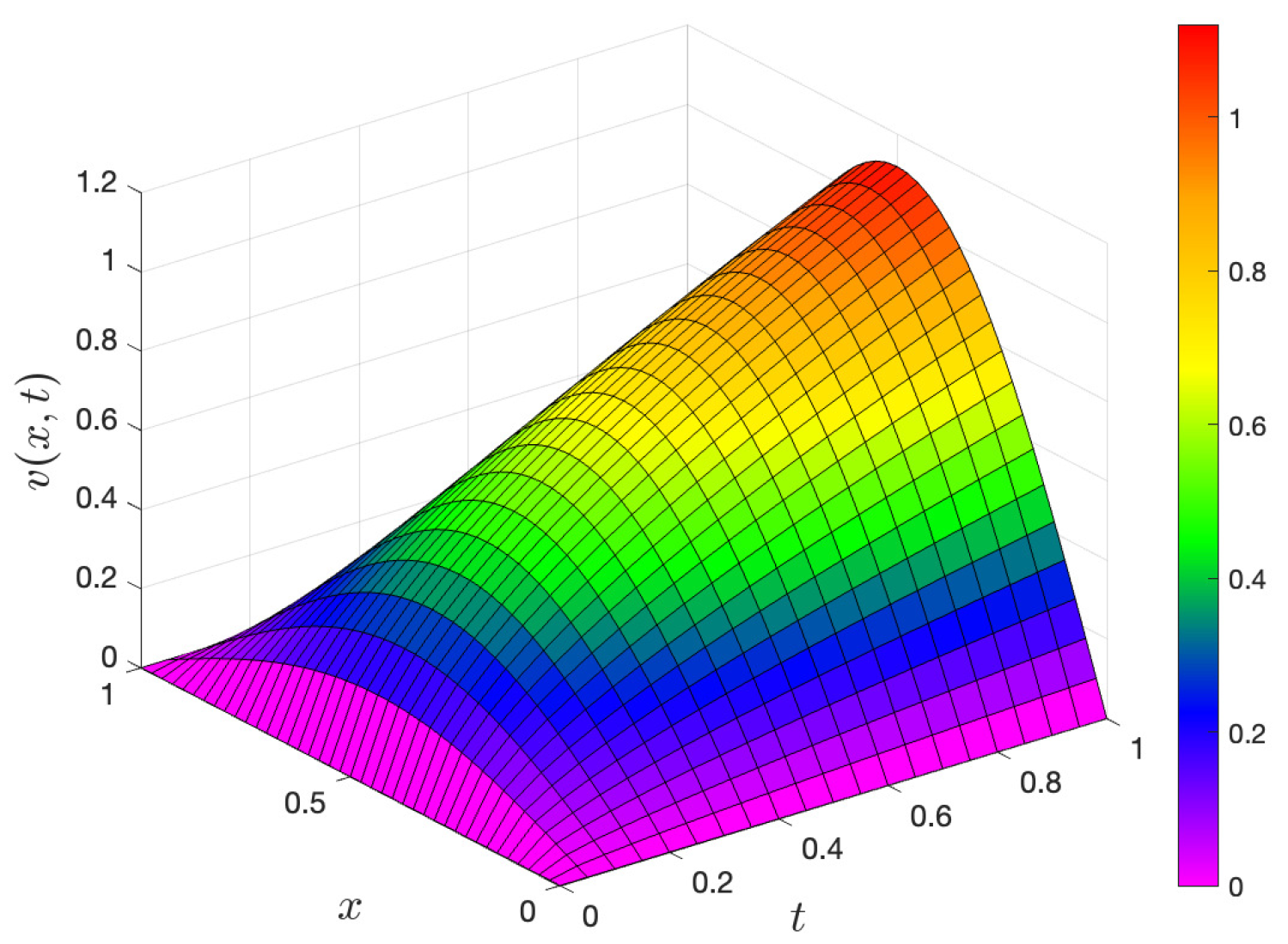
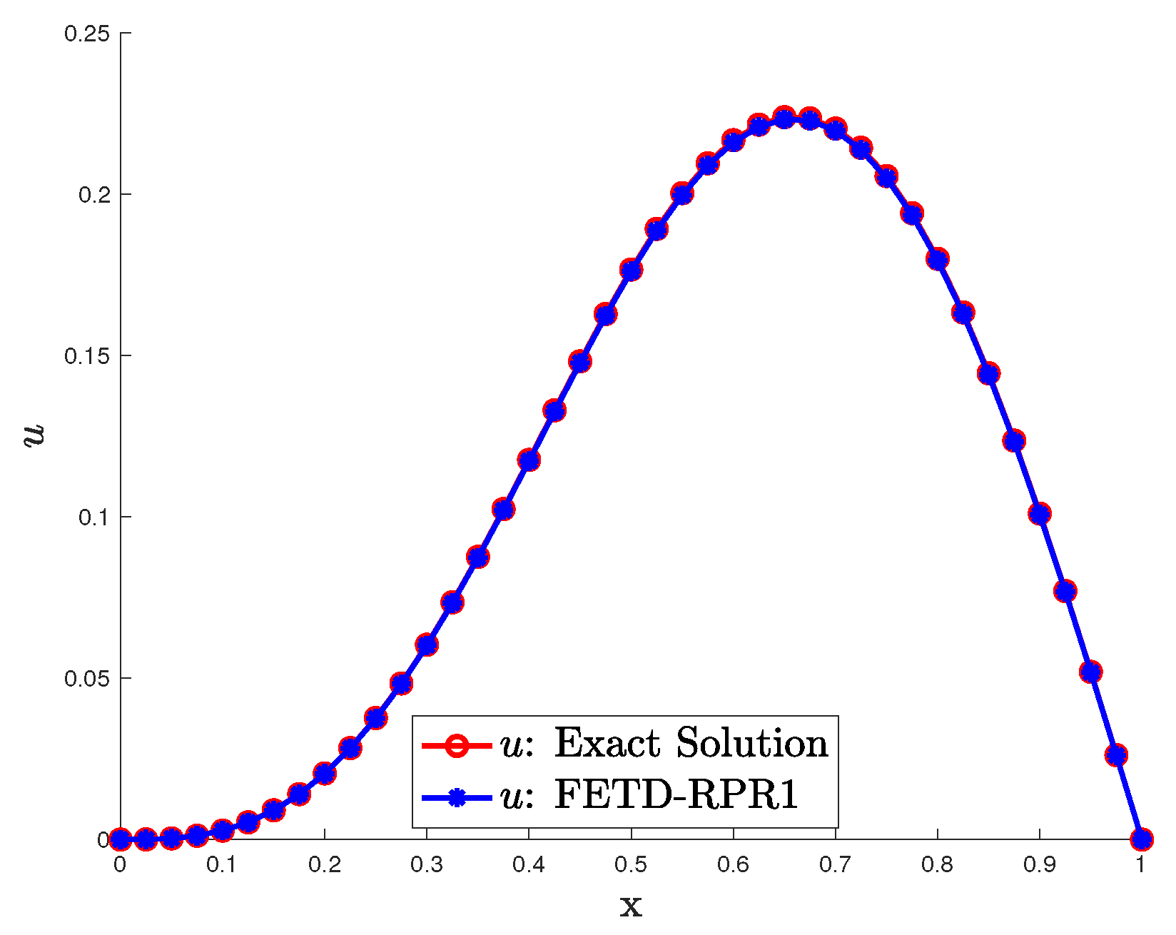
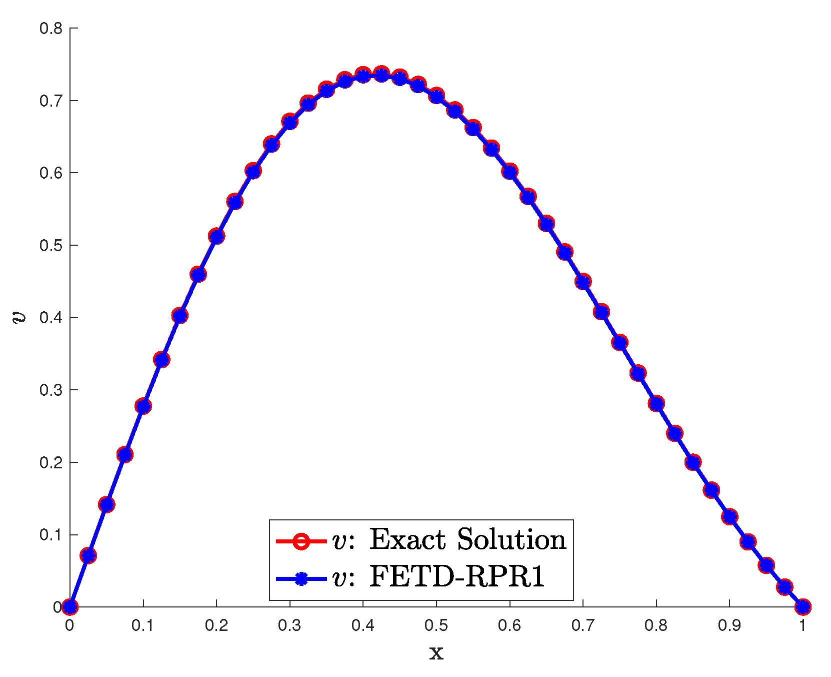
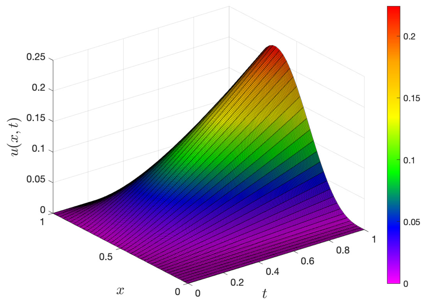
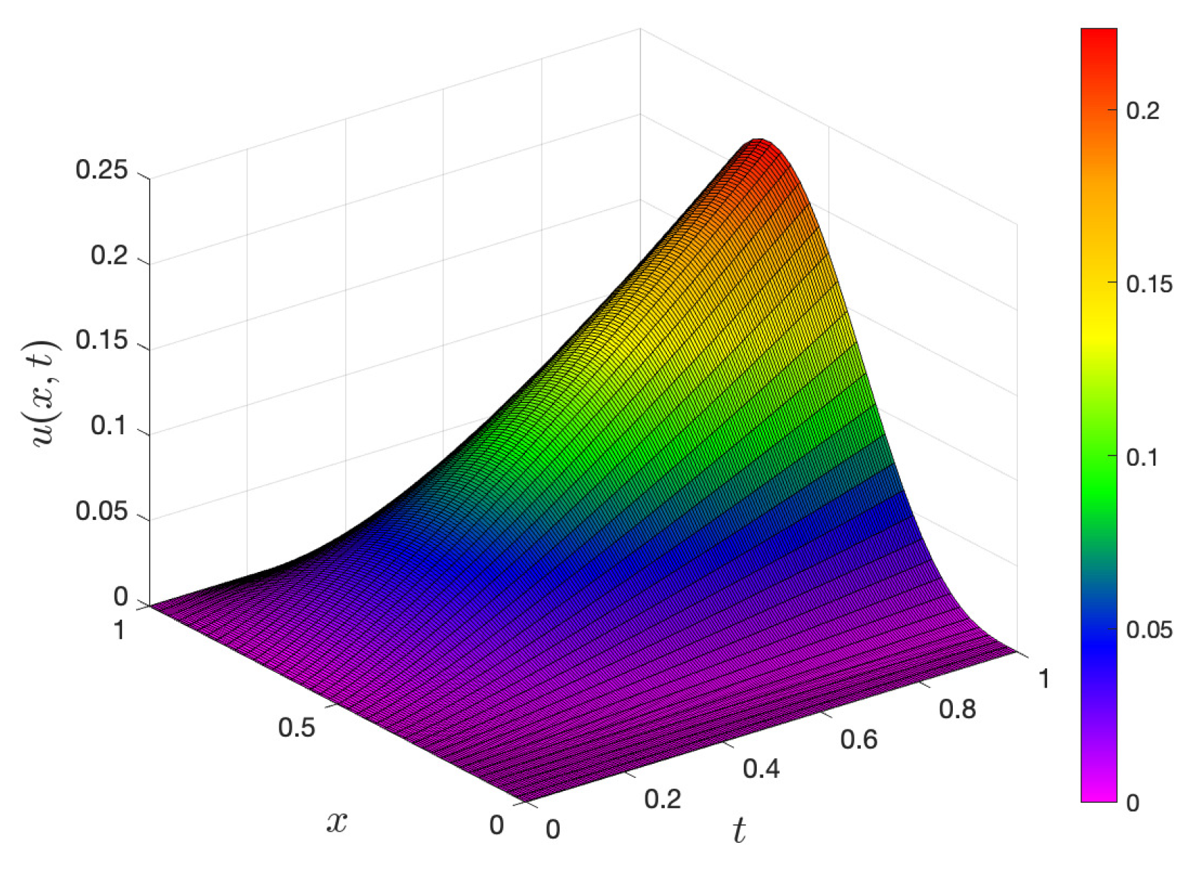
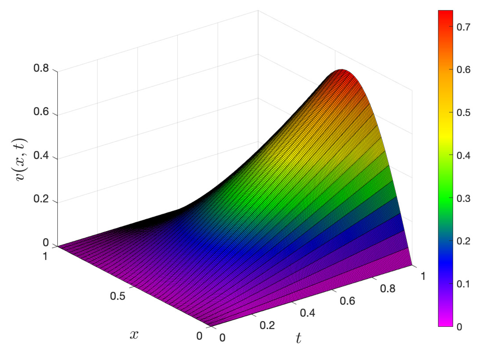
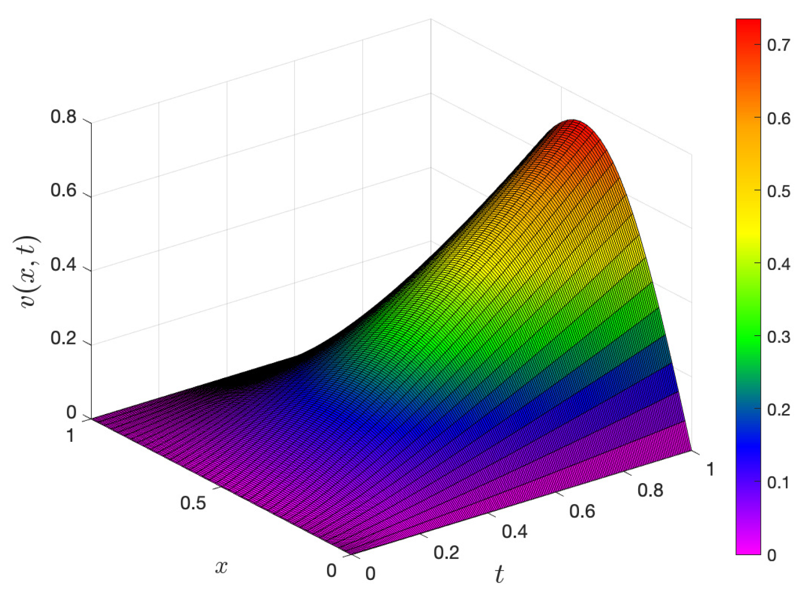
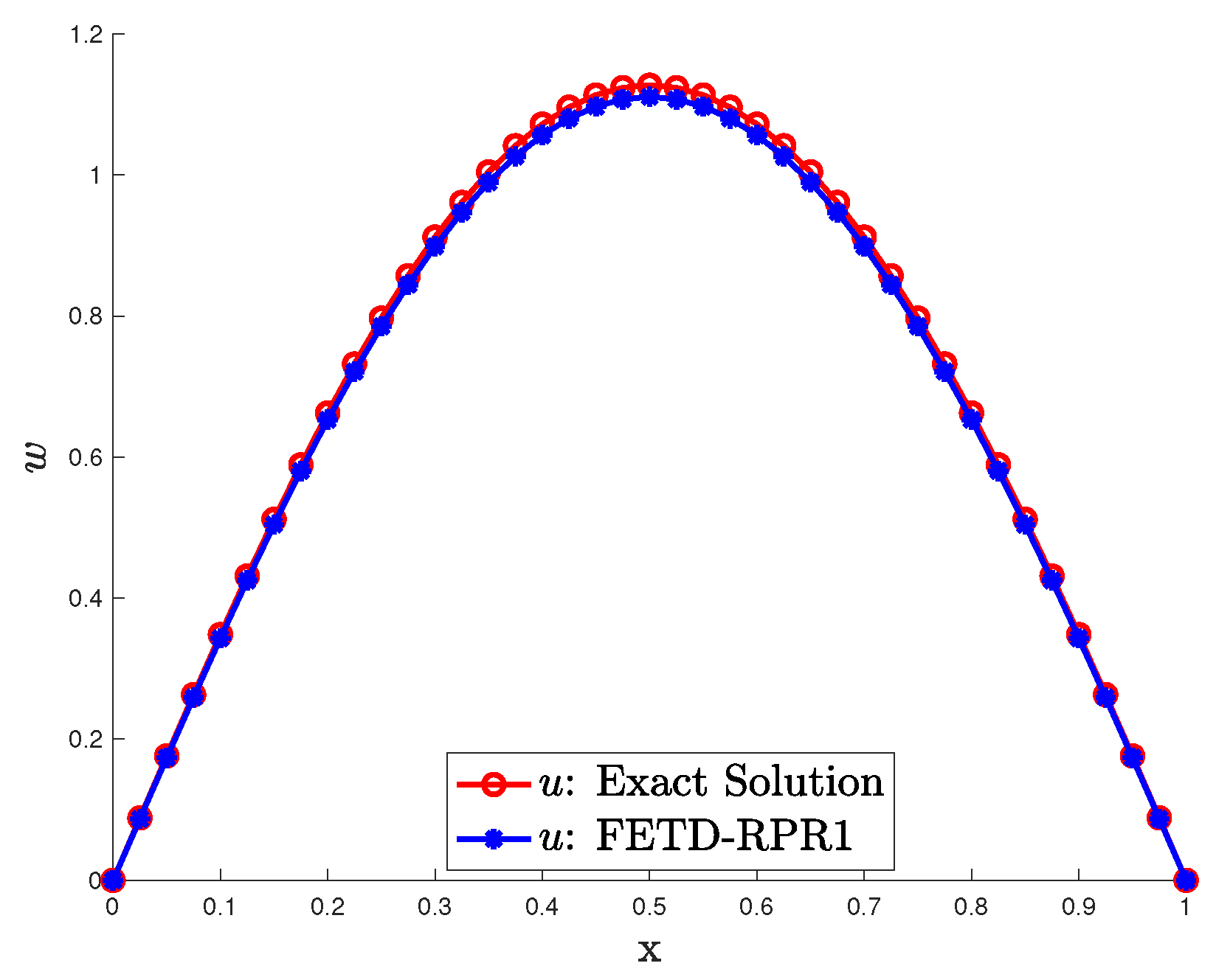
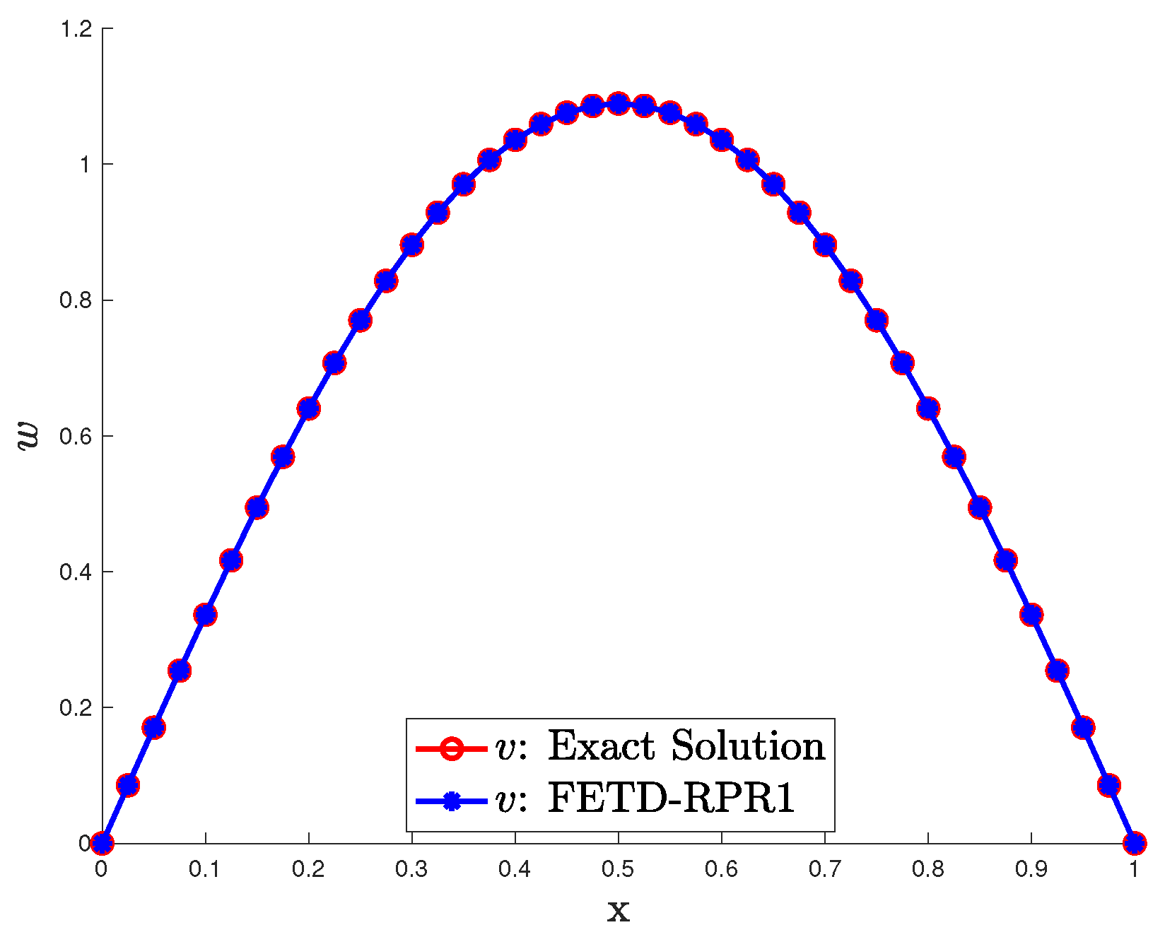
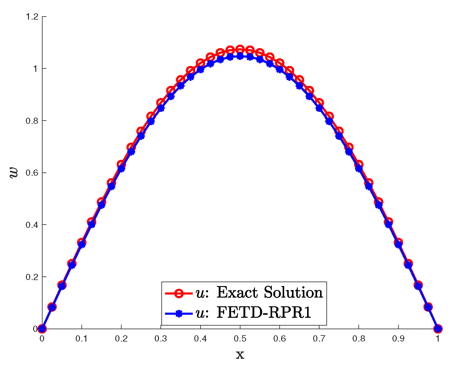
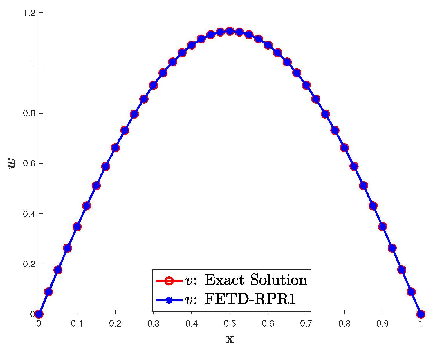
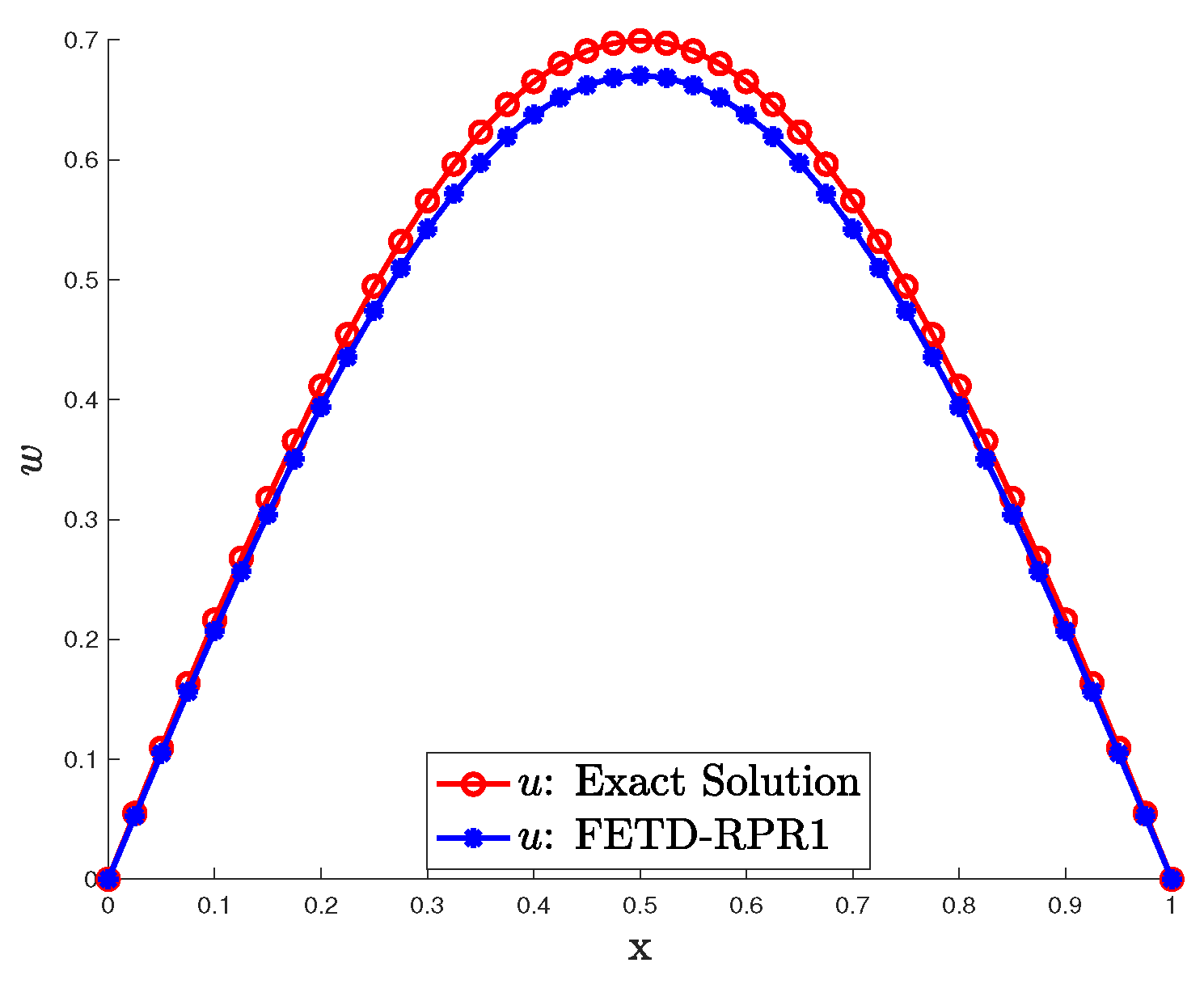
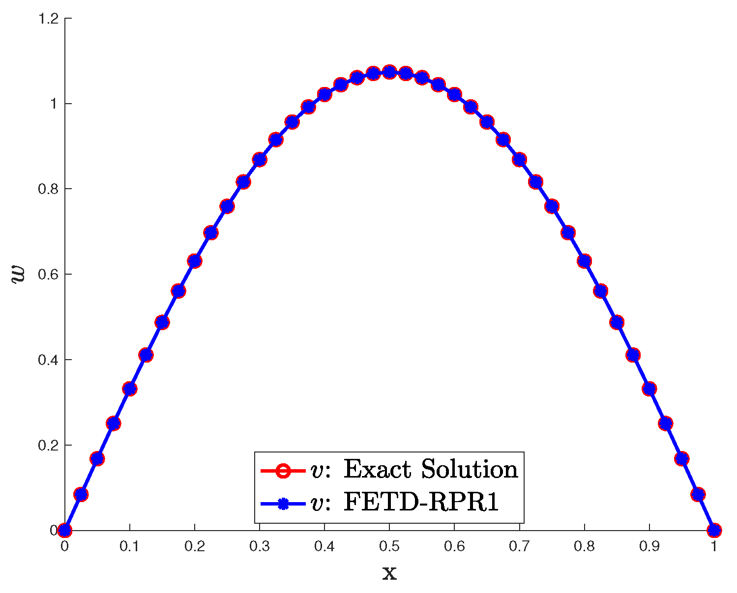
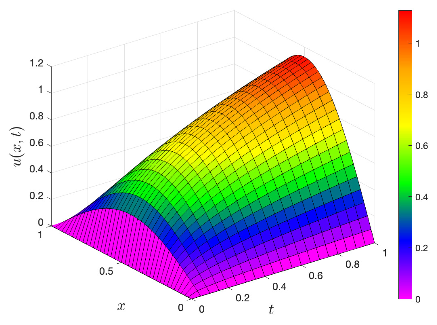
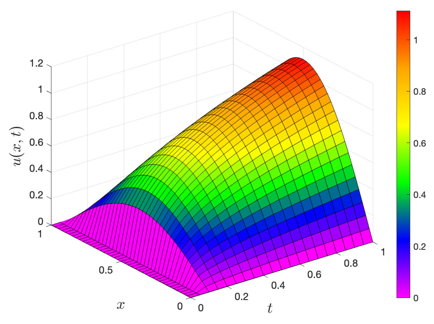
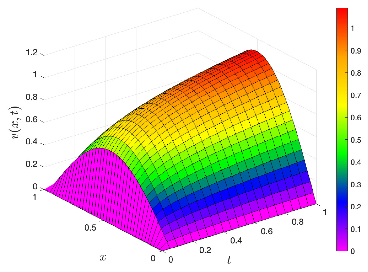
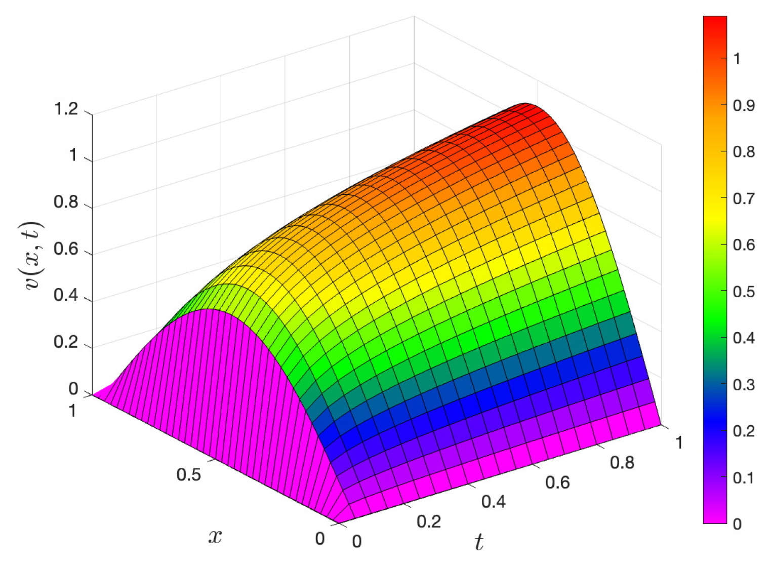
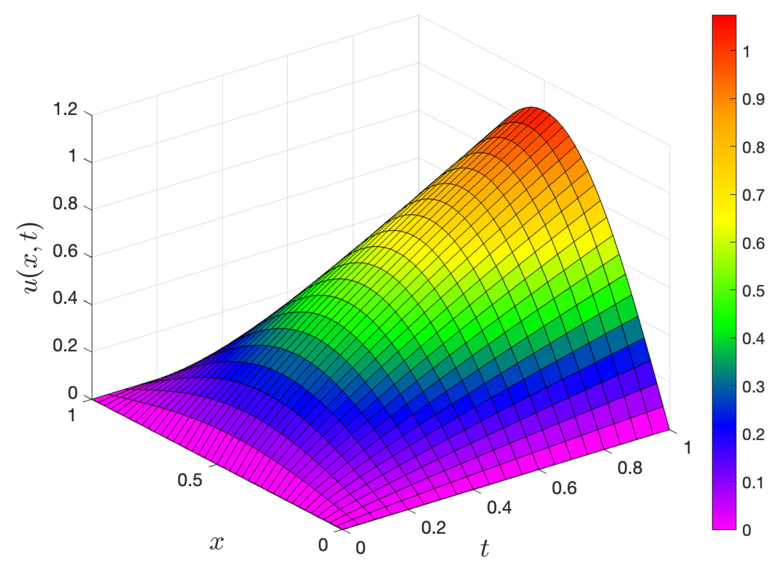
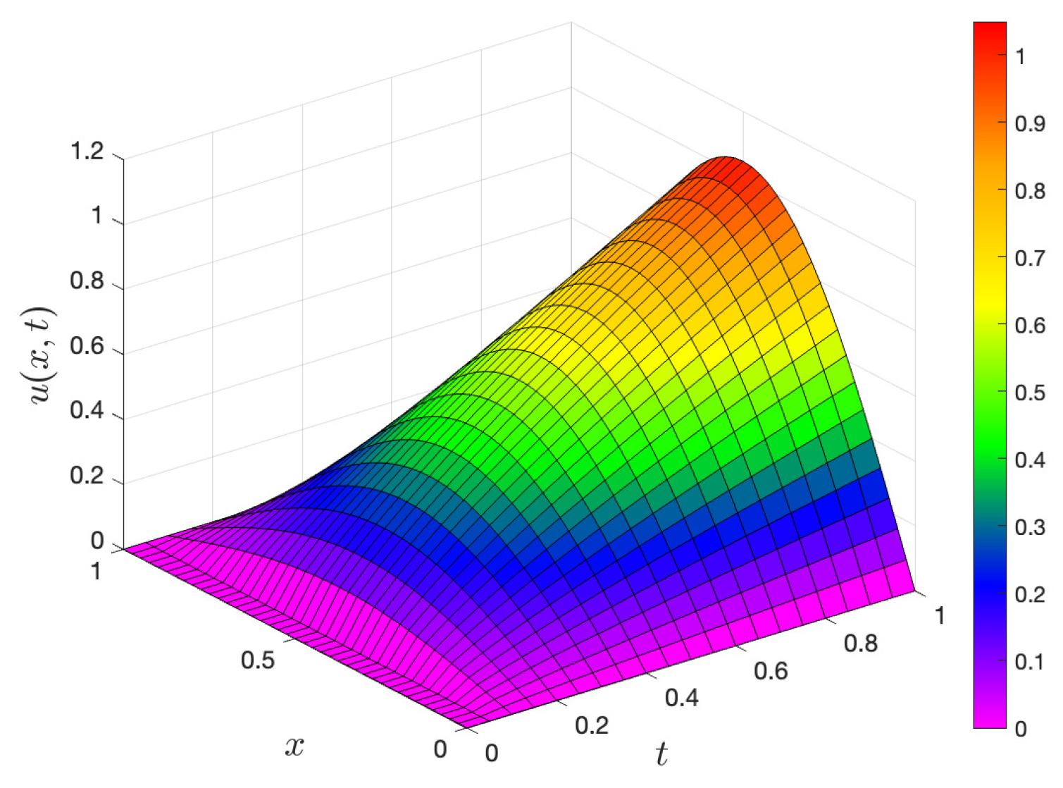
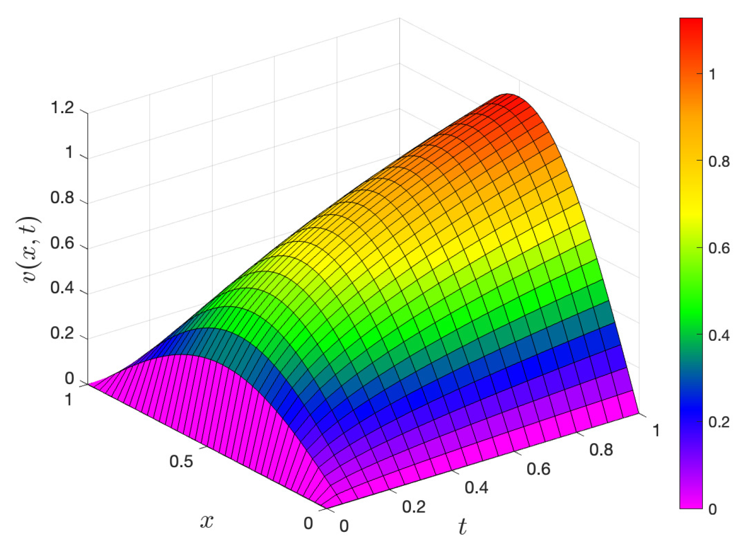
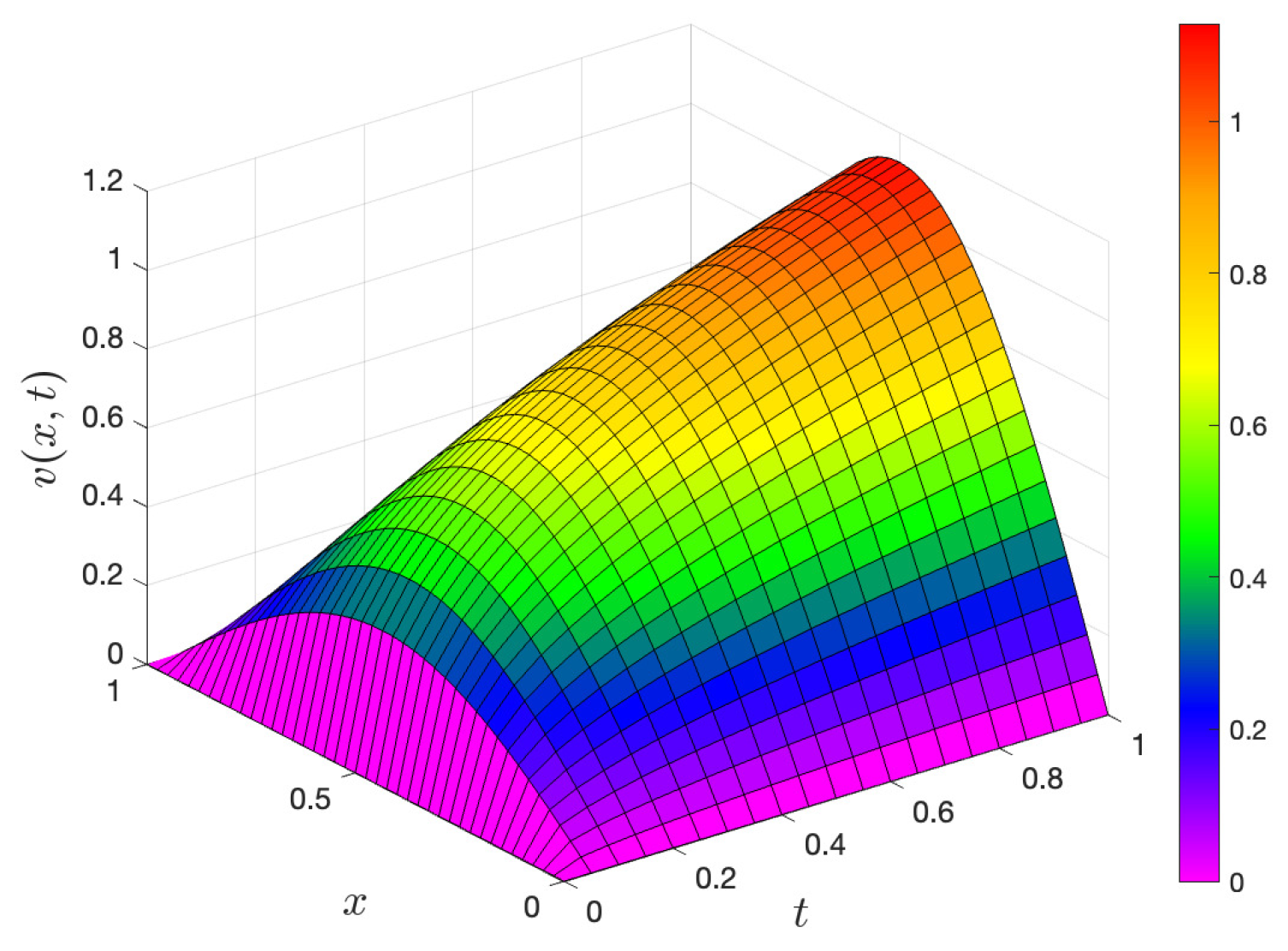
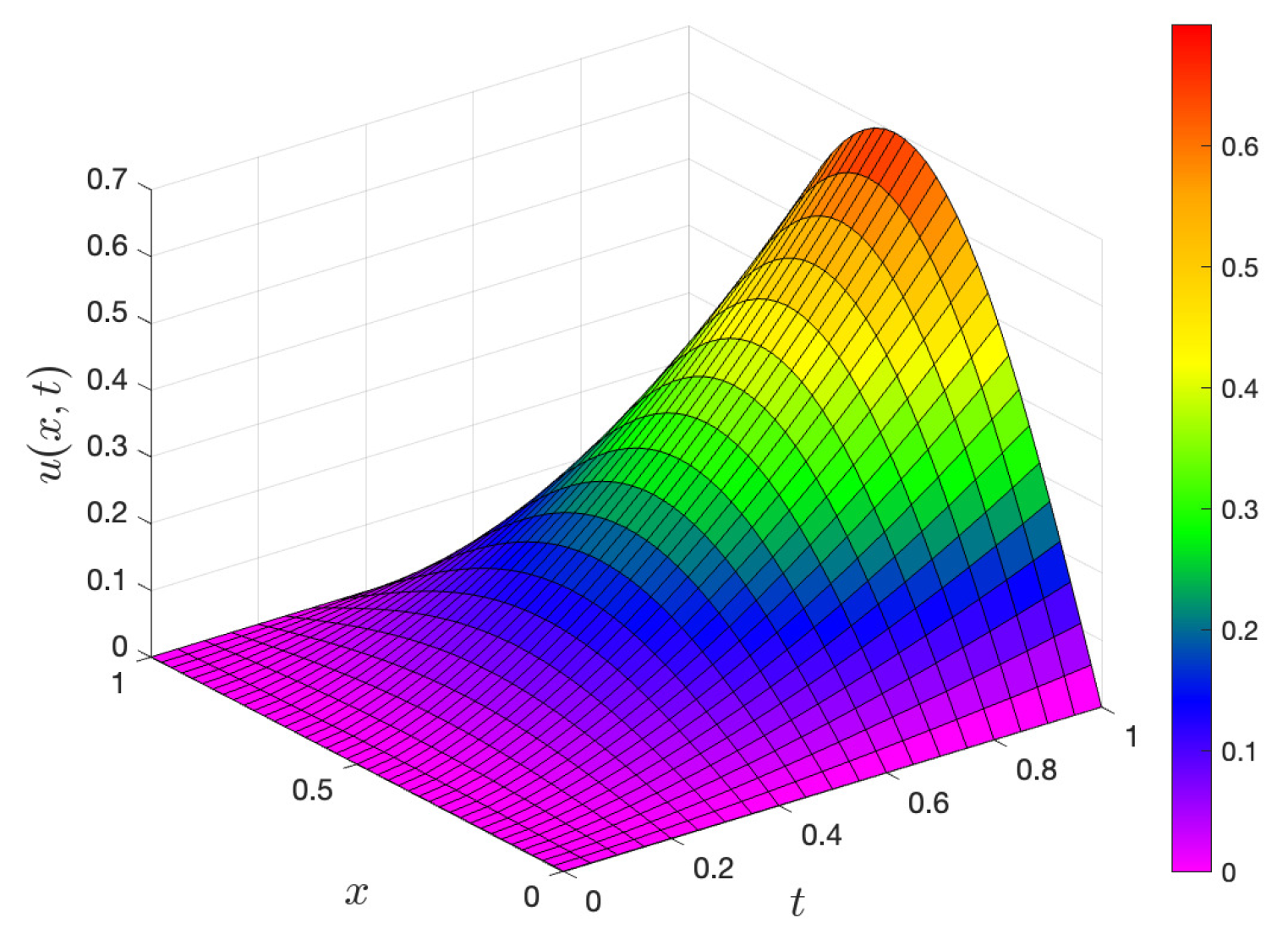
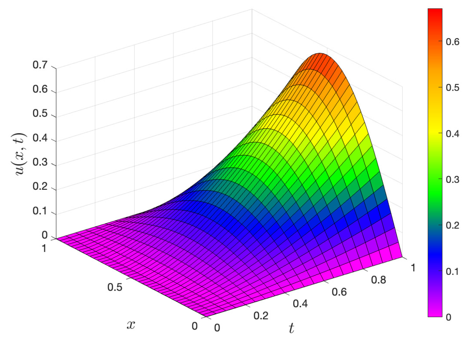
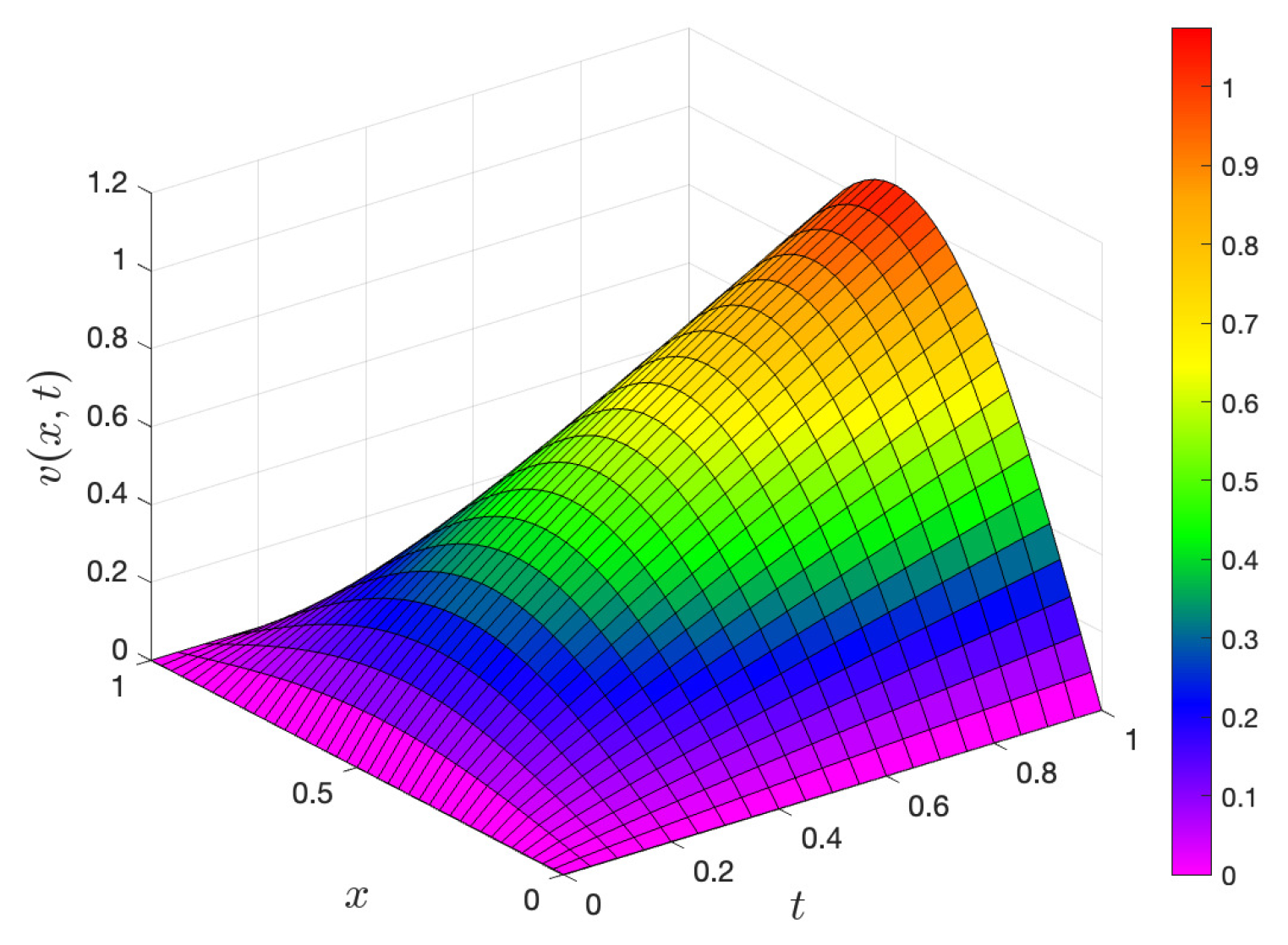
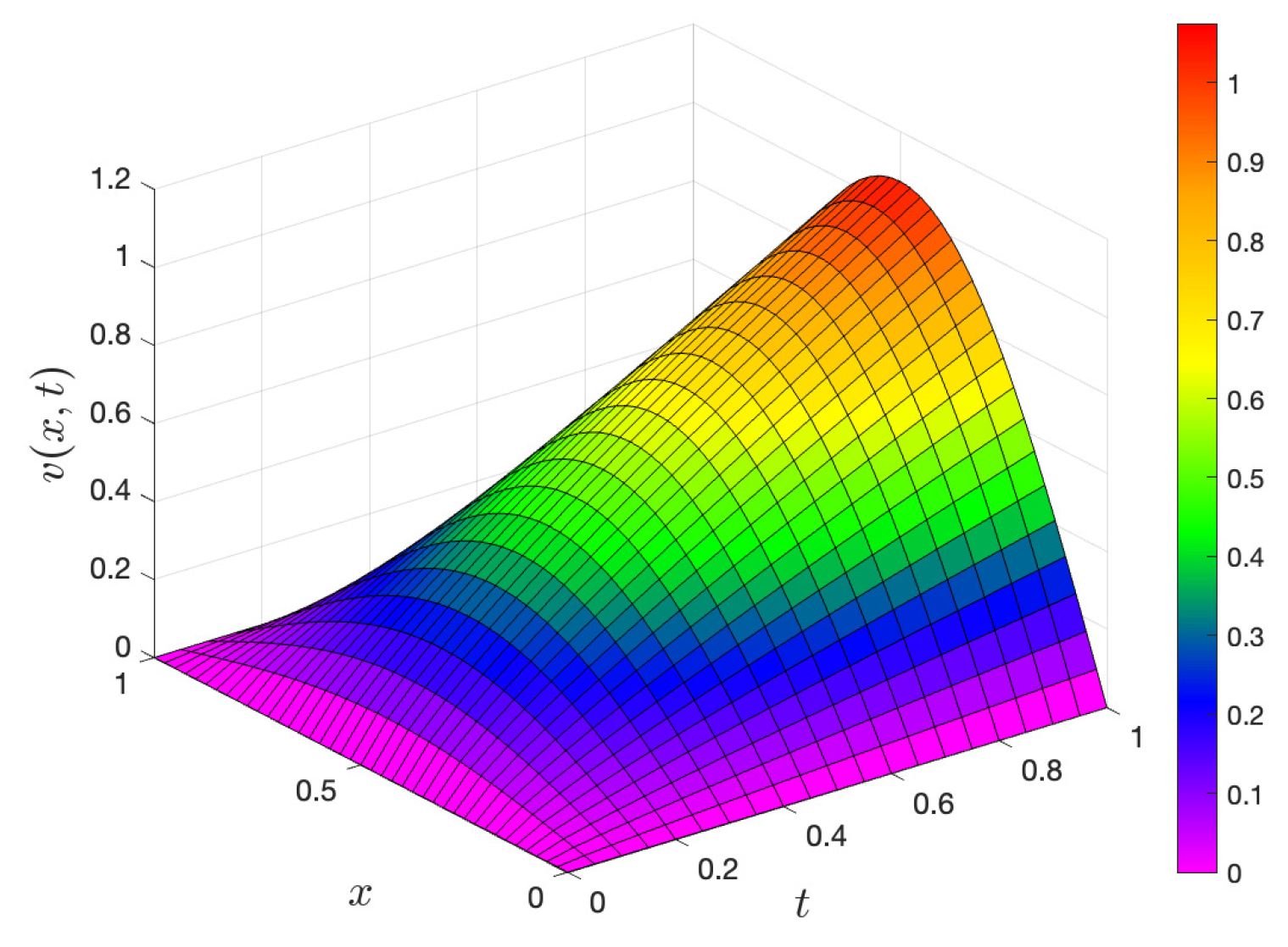
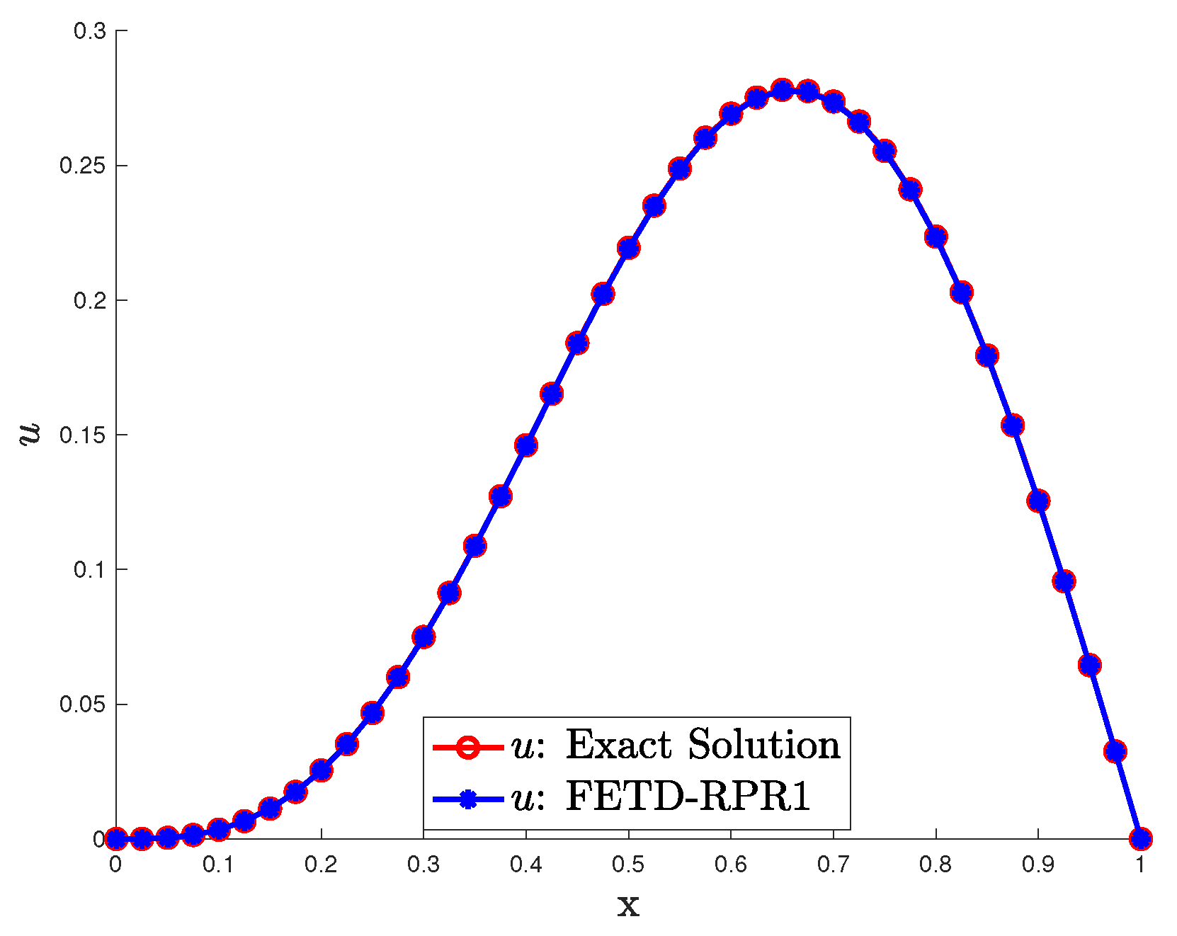
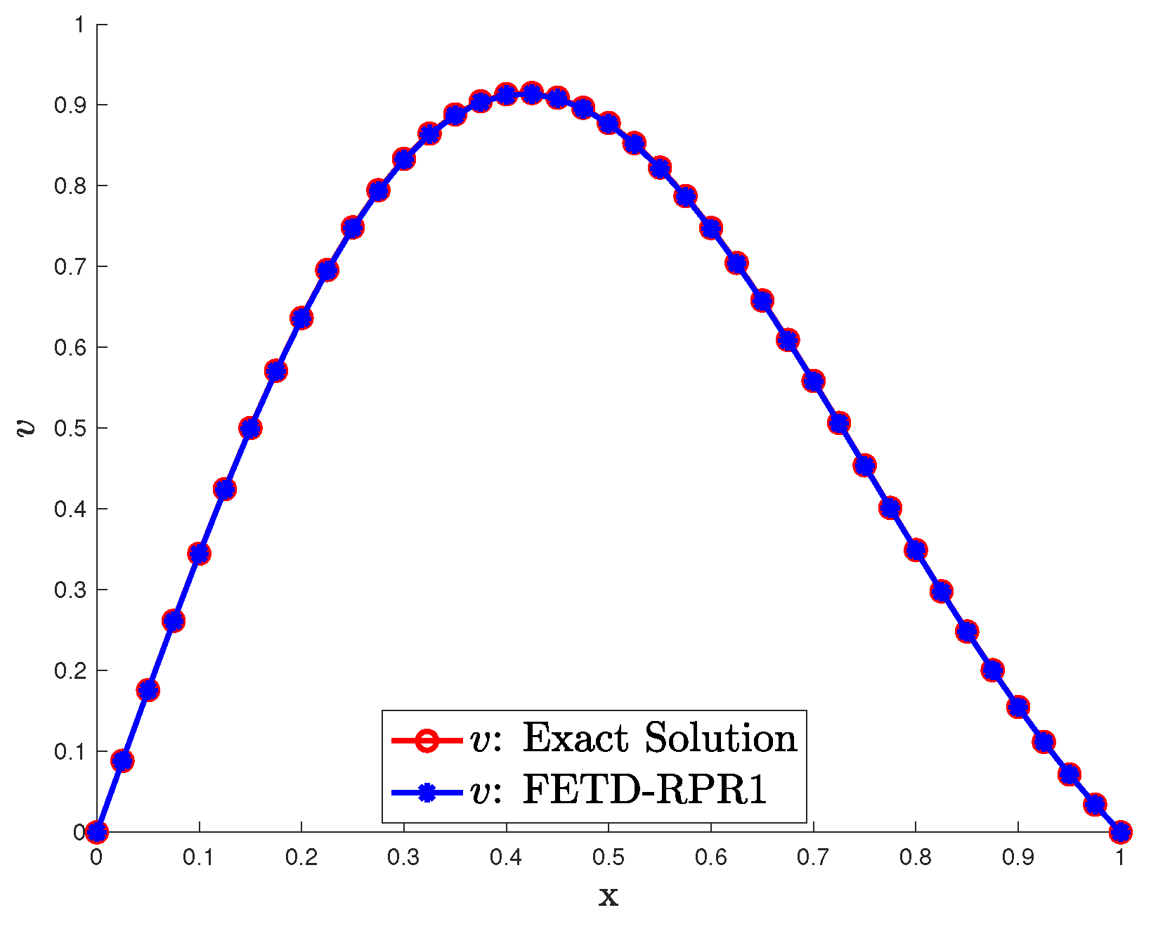
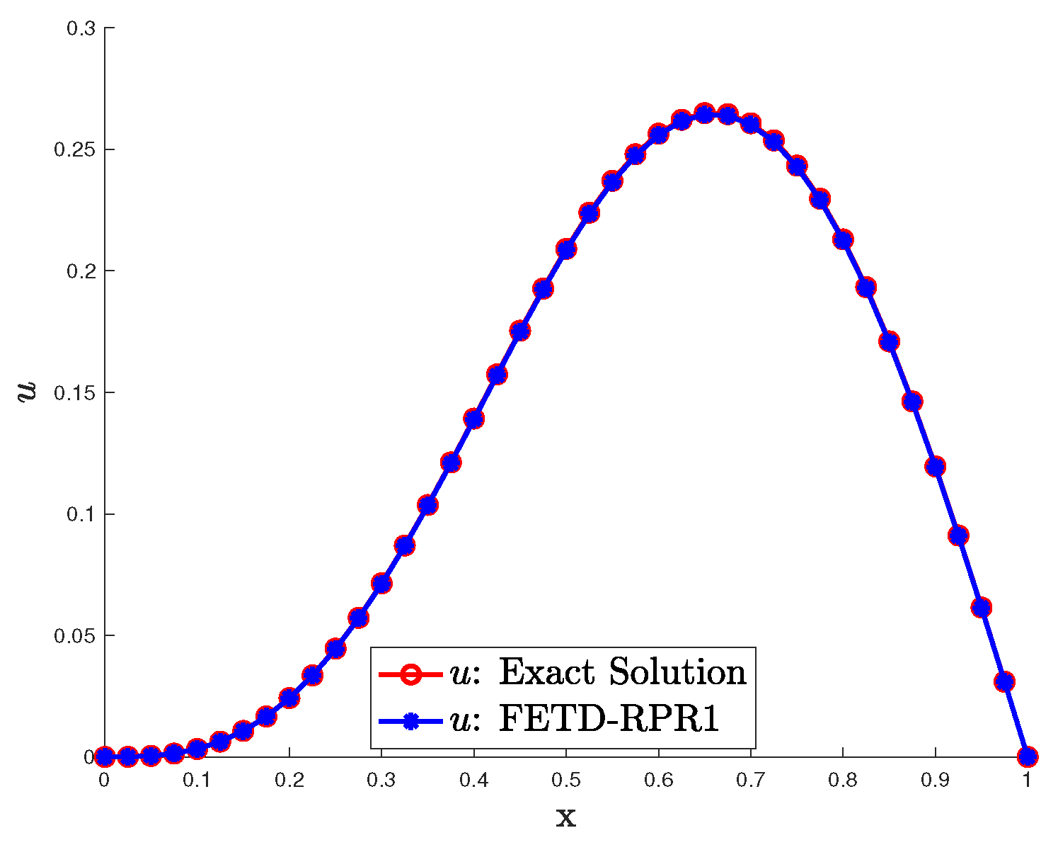
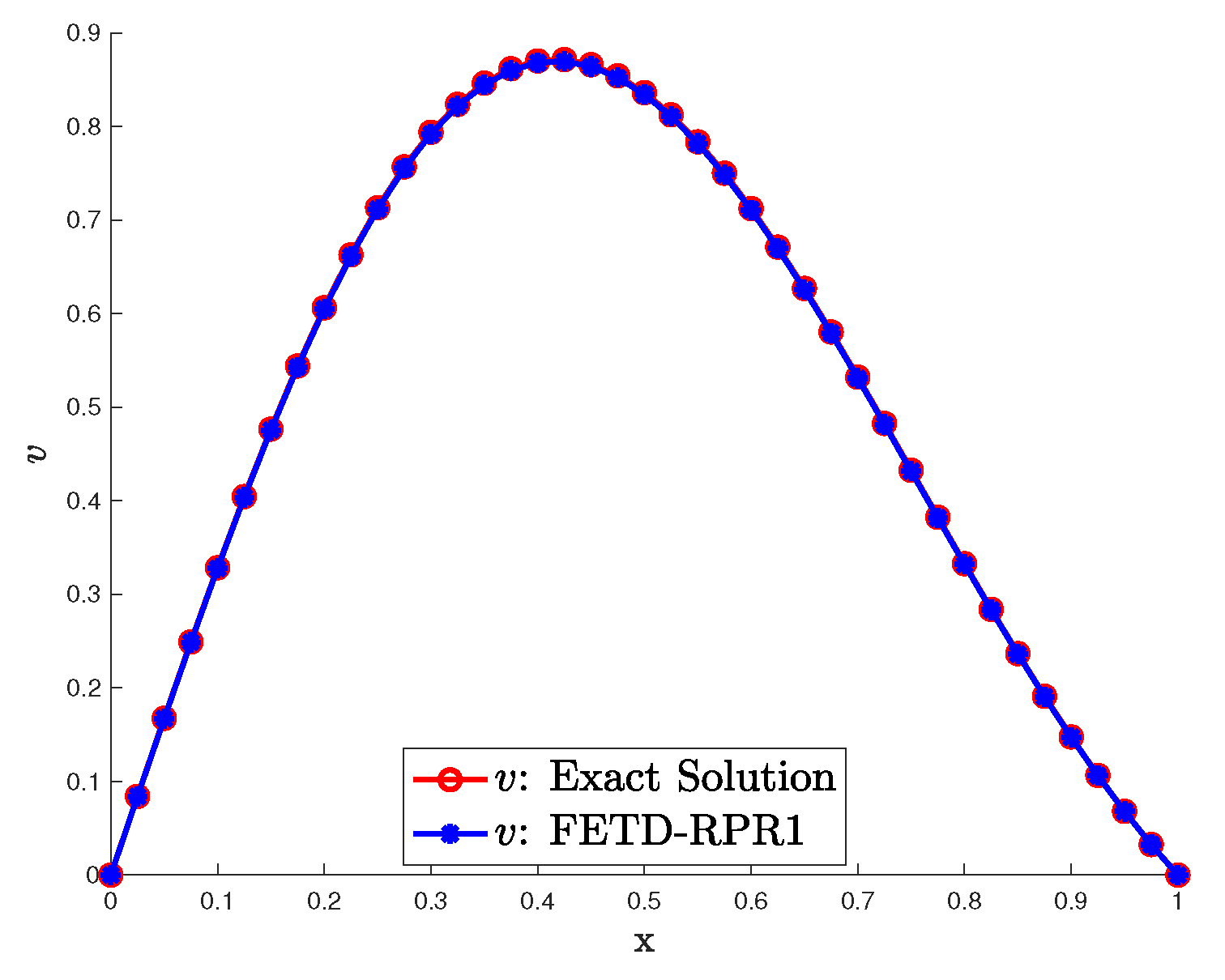
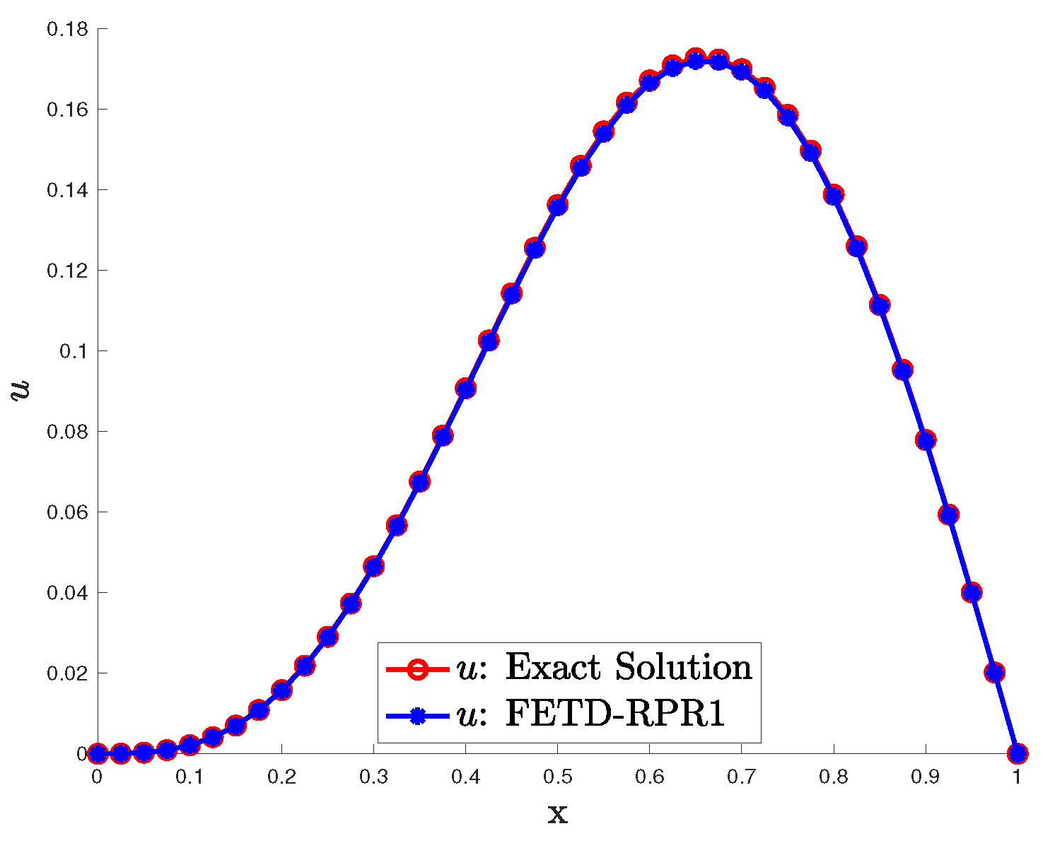
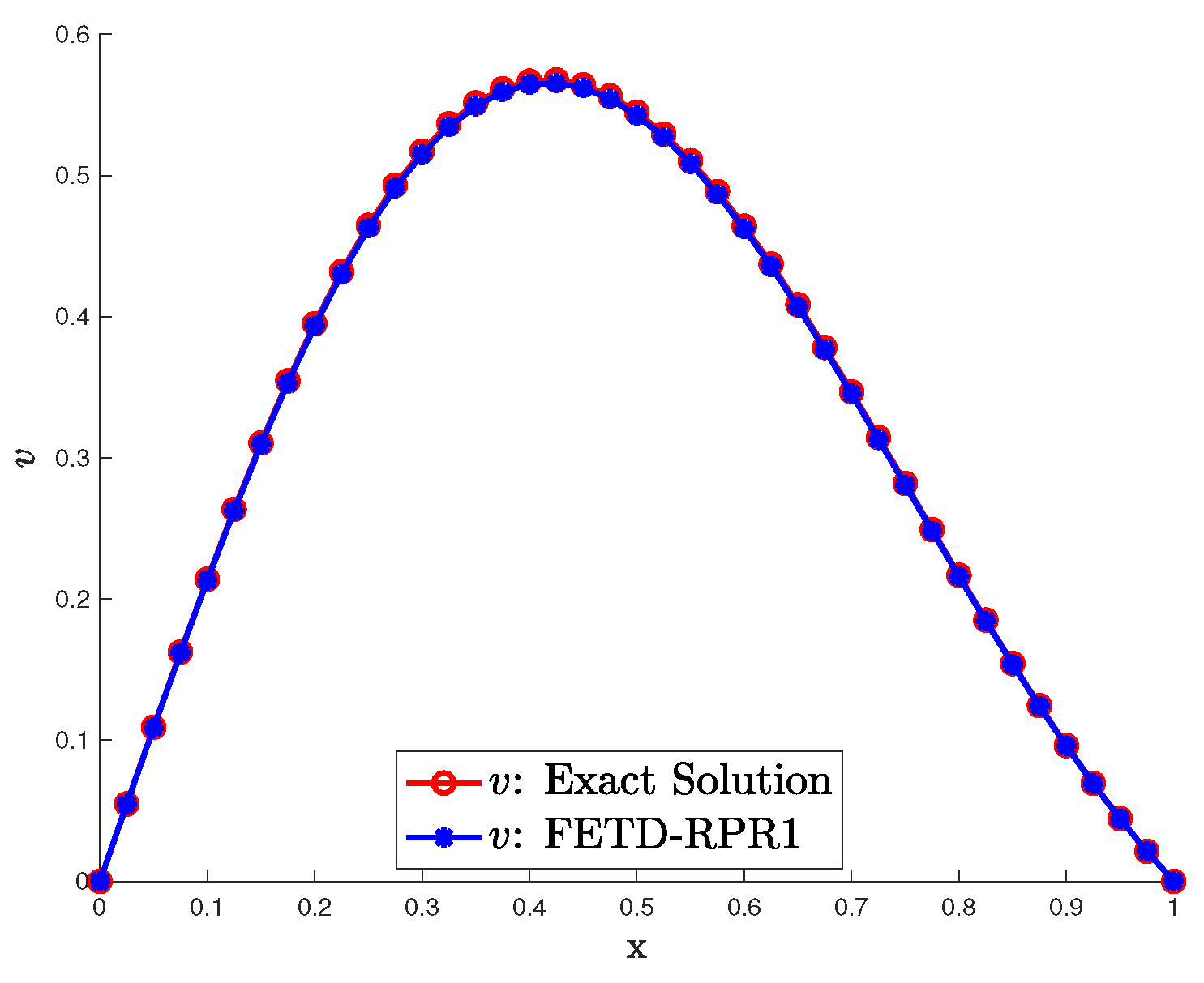
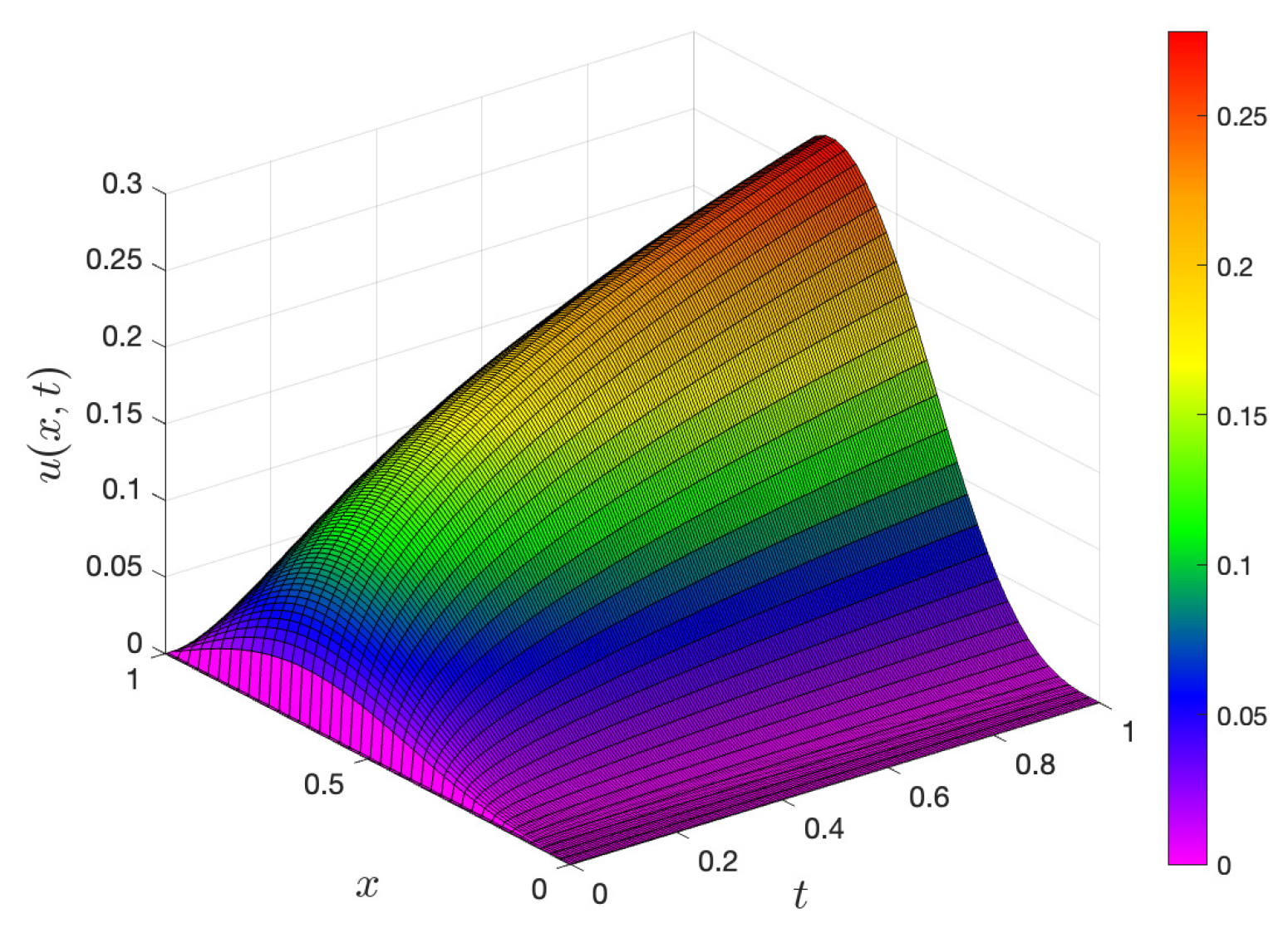
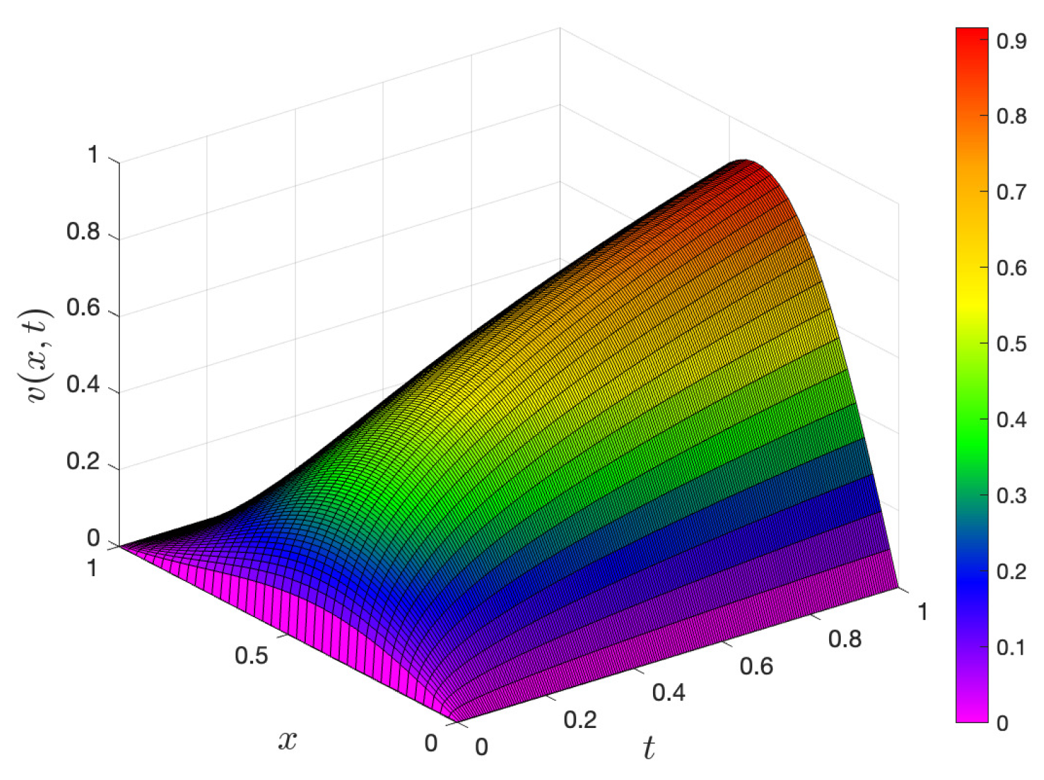
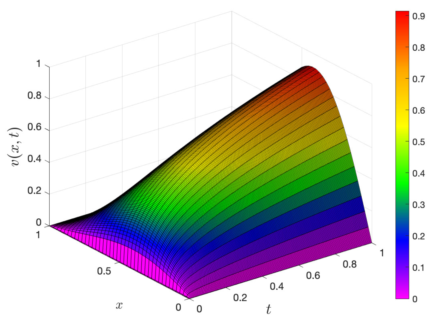
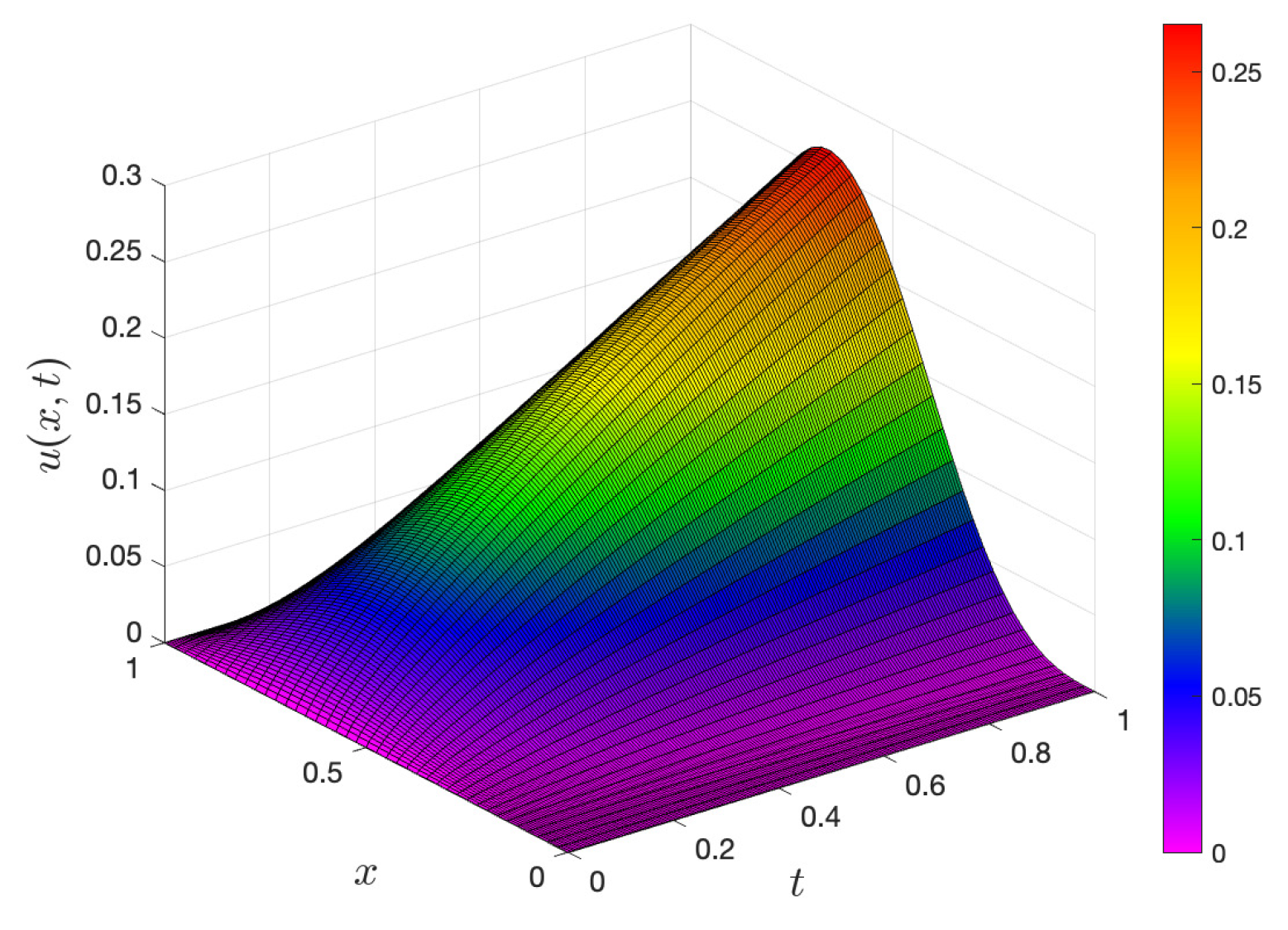
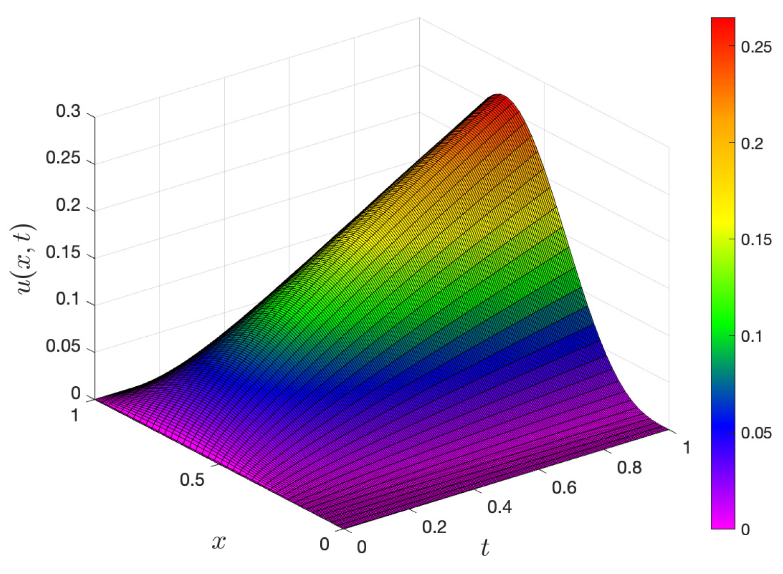
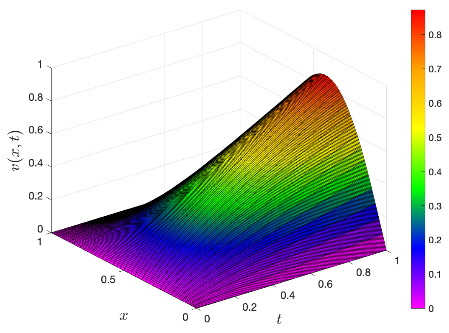
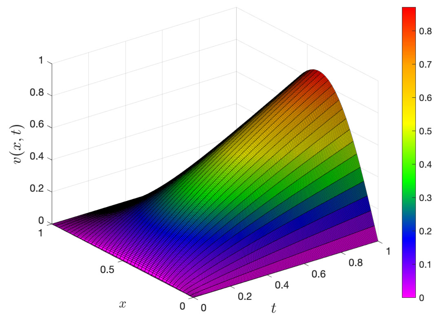
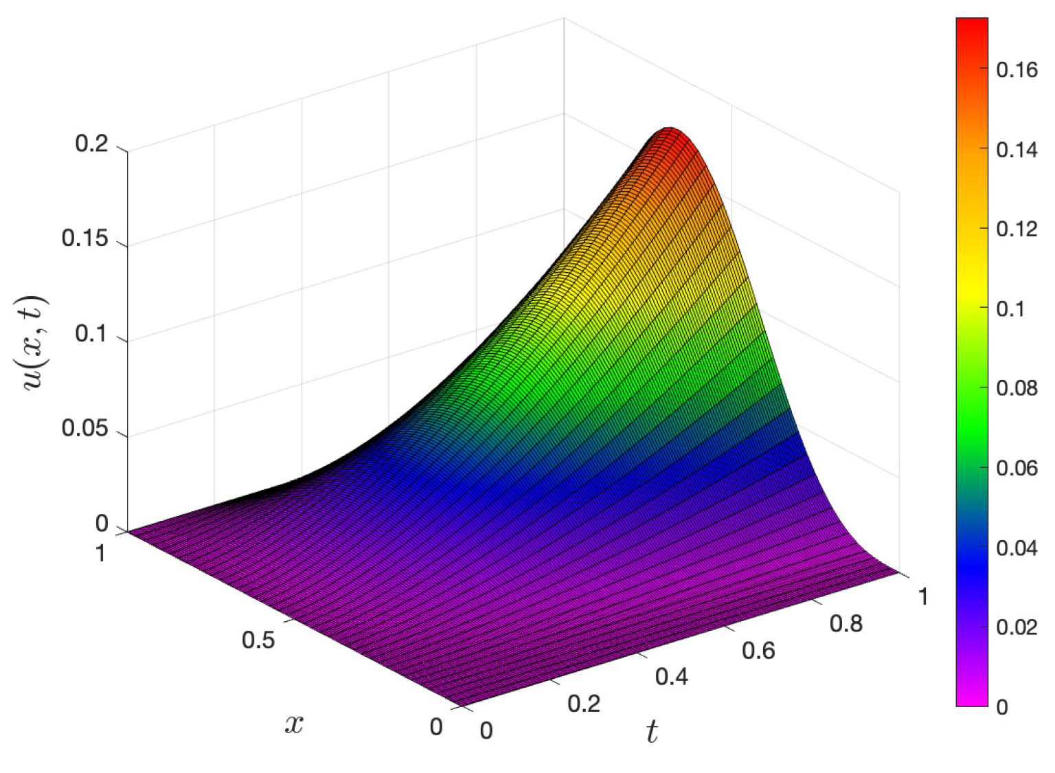
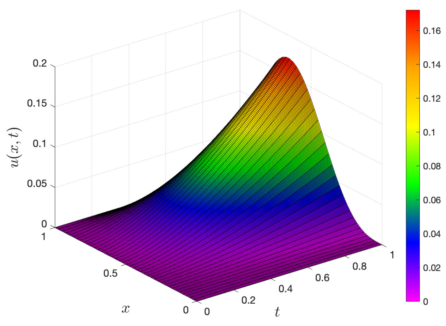
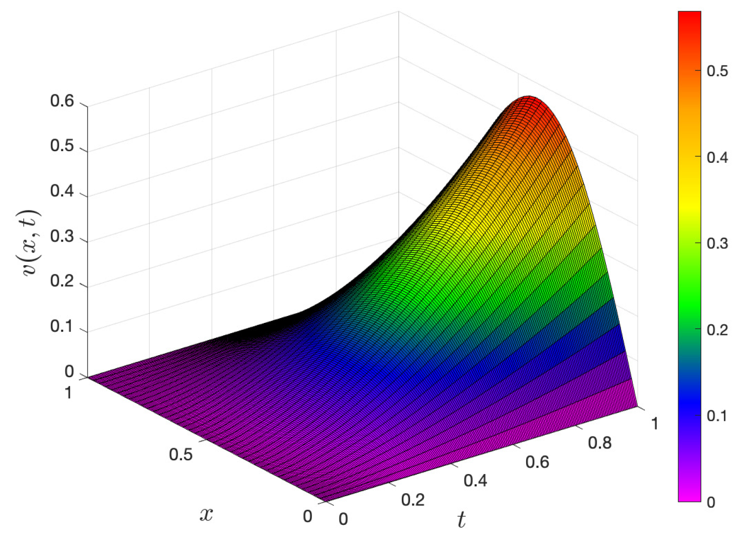
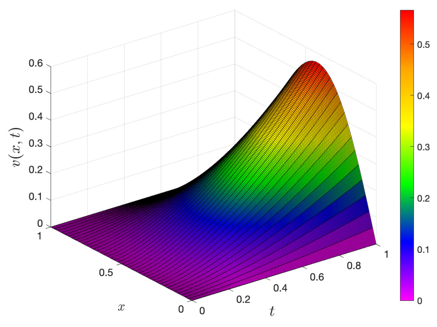
The qualitative behavior of the solutions for both components u and v is illustrated through the 2D and 3D plots in Figure 28 and Figure 29 (Appendix A, Figure A38, Figure A39, Figure A40, Figure A41, Figure A42 and Figure A43) and Figure 30, Figure 31, Figure 32 and Figure 33 (Appendix A, Figure A44, Figure A45, Figure A46, Figure A47, Figure A48, Figure A49, Figure A50, Figure A51, Figure A52, Figure A53, Figure A54 and Figure A55), respectively, for the time step $k=0.05$, spatial step size $h=0.025$, and final time $T=1$, with ${ϵ}_1=1\times {10}^{-3}$ and ${ϵ}_2=5\times {10}^{-4}$. These figures demonstrate a strong agreement between the numerical and exact solutions for both variables. In particular, the close overlap of the numerical and exact solution surfaces indicates that the proposed method accurately captures the coupled dynamics of the system.

Example 6.

Consider the following 1D linear system of time-fractional reaction–diffusion equations:

$$\begin{array}{ccc}\hfill {}^{c}D^{\sigma }u& =& {ϵ}_1{\displaystyle \frac{{\partial }^{2}u}{\partial x^2}}+f_1,t\ge 0,x\in [0,1],\hfill \\ \hfill {}^{c}D^{\sigma }v& =& {ϵ}_2{\displaystyle \frac{{\partial }^{2}v}{\partial x^2}}+f_2,\hfill \end{array}$$

where

$$\begin{array}{ccc}\hfill f_1& =& {ϵ}_1({\pi }^2-4x^2+10)u-2{ϵ}_{1}v-4\pi {ϵ}_1{\displaystyle \frac{t^{2\sigma }}{\mathrm{\Gamma }(2\sigma +1)}}x(1-x^2)\cos \left(\pi x\right)e^{-x^2}\hfill \\ & & +{\displaystyle \frac{t^{\sigma }}{\mathrm{\Gamma }(\sigma +1)}}{x}^2\sin \left(\pi x\right)e^{-x^2},\hfill \\ \hfill f_2& =& -4{ϵ}_{2}u+(2+{\pi }^2){ϵ}_{2}v+4\pi {ϵ}_2{\displaystyle \frac{t^{2\sigma }}{\mathrm{\Gamma }(2\sigma +1)}}x\cos \left(\pi x\right)e^{-x^2}+{\displaystyle \frac{t^{\sigma }}{\mathrm{\Gamma }(\sigma +1)}}\sin \left(\pi x\right)e^{-x^2},\hfill \end{array}$$

with the exact solution

$$\begin{array}{ccc}\hfill u(x,t)& =& {\displaystyle \frac{t^{2\sigma }}{\mathrm{\Gamma }(2\sigma +1)}}{x}^2\sin \left(\pi x\right)e^{-x^2},\hfill \\ \hfill v(x,t)& =& {\displaystyle \frac{t^{2\sigma }}{\mathrm{\Gamma }(2\sigma +1)}}\sin \left(\pi x\right)e^{-x^2}.\hfill \end{array}$$

The numerical results for Example 6, including the computed errors, order of convergence, and CPU time, are presented in

Table 6. Numerical results for Example 6.

$\mathit{\sigma }$	k	h	Error	OC	CPU Time
0.2	0.0200	0.016393	$4.9952\times {10}^{-3}$	-	$2.3139\times {10}^{-1}$
	0.0100	0.016393	$2.4022\times {10}^{-3}$	1.06	$5.9512\times {10}^{-1}$
	0.0050	0.016393	$1.1574\times {10}^{-3}$	1.05	$2.2081$
	0.0025	0.016393	$5.5641\times {10}^{-3}$	$1.06$	$8.5063$
0.4	0.0200	0.016393	$7.9393\times {10}^{-3}$	-	$1.4894\times {10}^{-1}$
	0.0100	0.016393	$3.8499\times {10}^{-3}$	1.04	$5.7570\times {10}^{-1}$
	0.0050	0.016393	$1.8741\times {10}^{-3}$	1.04	$2.1284$
	0.0025	0.016393	$9.1167\times {10}^{-3}$	$1.04$	$9.0951$
0.6	0.0200	0.016393	$9.3278\times {10}^{-3}$	-	$1.4789\times {10}^{-1}$
	0.0100	0.016393	$4.5876\times {10}^{-3}$	1.02	$5.6805\times {10}^{-1}$
	0.0050	0.016393	$2.2628\times {10}^{-3}$	1.02	$2.1987$
	0.0025	0.016393	$1.1155\times {10}^{-3}$	1.02	$8.8114$
0.8	0.1000	0.016393	$9.2752\times {10}^{-3}$	-	$1.5688\times {10}^{-1}$
	0.0500	0.016393	$4.6076\times {10}^{-3}$	1.01	$5.6680\times {10}^{-1}$
	0.0250	0.016393	$2.2914\times {10}^{-3}$	1.01	$2.3220$
	0.0125	0.016393	$1.1385\times {10}^{-3}$	1.01	$8.9686$

for the selected parameters ${ϵ}_1=1\times {10}^{-2}$ and ${ϵ}_2=1\times {10}^{-3}$. The tabulated results demonstrate a consistent decrease in numerical error with grid refinement, indicating the accuracy and stability of the proposed scheme. Despite the complexity of the coupled nonlinear system, the method maintains reliable performance in terms of both precision and computational efficiency.

The convergence behavior is further illustrated in Figure 34 (Appendix A, Figure A56), where the numerical results clearly exhibit first-order convergence. The agreement between the observed convergence rates in the plots and those reported in Table 6 confirms the theoretical expectations and validates the effectiveness of the method for solving such systems.

Moreover, the qualitative behavior of the solutions for the variables u and v is demonstrated through the 2D and 3D solution plots shown in Figure 35 and Figure 36 (Appendix A, Figure A57, Figure A58, Figure A59, Figure A60, Figure A61 and Figure A62) and Figure 37, Figure 38, Figure 39 and Figure 40 (Appendix A, Figure A63, Figure A64, Figure A65, Figure A66, Figure A67, Figure A68, Figure A69, Figure A70, Figure A71, Figure A72, Figure A73 and Figure A74), respectively. These results are obtained for ${ϵ}_1=1\times {10}^{-3}$, ${ϵ}_2=5\times {10}^{-4}$, $T=1$, $k=5\times {10}^{-3}$, and $h=0.025$. The graphical comparisons reveal an excellent agreement between the numerical and exact solutions for both components.

Comparison Tests

In this subsection, we concentrate on comparing the efficiency of our proposed algorithm with the first-order L1 scheme [55]. The L1 scheme is formulated using the L1 discretization of the Caputo fractional derivative and employs a second-order central difference for the spatial discretization of the Laplacian operator. The L1 discretization of the Caputo fractional derivative [54] is defined as

$$\begin{array}{ccc}\hfill {}^{c}D^{\sigma }W\left(t_n\right)& =& {\displaystyle \frac{1}{\mathrm{\Gamma }(2-\sigma )}}{\displaystyle \sum _{j=0}^{n-1}}{\displaystyle \frac{W_{j+1}-W_j}{k}}[{(t_n-t_j)}^{1-\sigma }-{(t_n-t_{j+1})}^{1-\sigma }].\hfill \end{array}$$

Equivalently, we have

$$\begin{array}{cc}{}^{c}D^{\sigma }W\left(t_n\right)\hfill & ={\displaystyle \frac{k^{-\sigma }}{\mathrm{\Gamma }(2-\sigma )}}{\displaystyle \sum _{j=0}^{n-1}}[{(n-j)}^{1-\sigma }-{(n-j-1)}^{1-\sigma }]\left(W_{j+1}-W_j\right)\hfill \\ & =k^{-\sigma }{\displaystyle \sum _{k=0}^{n-1}}{w}_k^{\sigma }(W_{n-k}-W_{n-k-1}),\hfill \end{array}$$

(37)

where

$${\displaystyle w_k^{\sigma }=\frac{{(k+1)}^{1-\sigma }-k^{1-\sigma }}{\mathrm{\Gamma }(2-\sigma )}.}$$

Using Equation (37) and Laplacian discretization over the spatial domain $\mathrm{\Omega }=[a,b]$ with mesh $x_i=a+ih,i=0,1,\dots ,M$, we observe the explicit variant of the L1 scheme as

$$\begin{array}{c}{W}_i^n={\displaystyle \frac{k^{\sigma }}{w_0}}\left({\displaystyle \frac{W_{i-1}^{n-1}-2W_i^{n-1}+W_{i+1}^{n-1}}{h^2}}+\mathcal{H}(W_i^{n-1},t_{n-1})\right)+W_i^{n-1}\hfill \\ \hfill \\ -{\displaystyle \frac{1}{w_0}}{\displaystyle \sum _{k=0}^{n-1}}{w}_k^{\sigma }(W_i^{n-k}-W_i^{n-k-1}),i=1,2,\dots ,M-1,\hfill \end{array}$$

(38)

where

$${\displaystyle w_0=\frac{1}{\mathrm{\Gamma }(2-\sigma )},w_k^{\sigma }=\frac{{(k+1)}^{1-\sigma }-k^{1-\sigma }}{\mathrm{\Gamma }(2-\sigma )}}$$

and $W_i^n$ approximates $W(x_i,t_n).$ The algorithm for the L1 method is represented below.

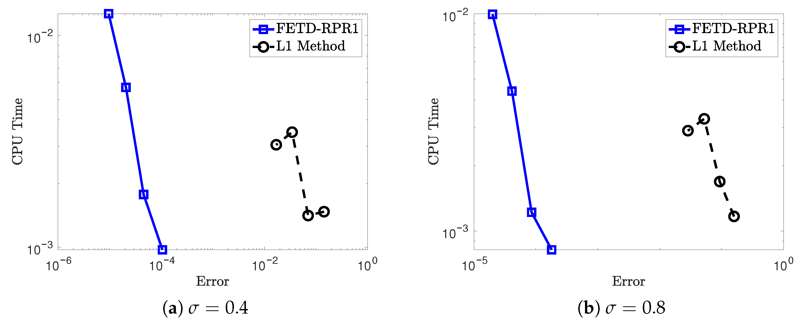
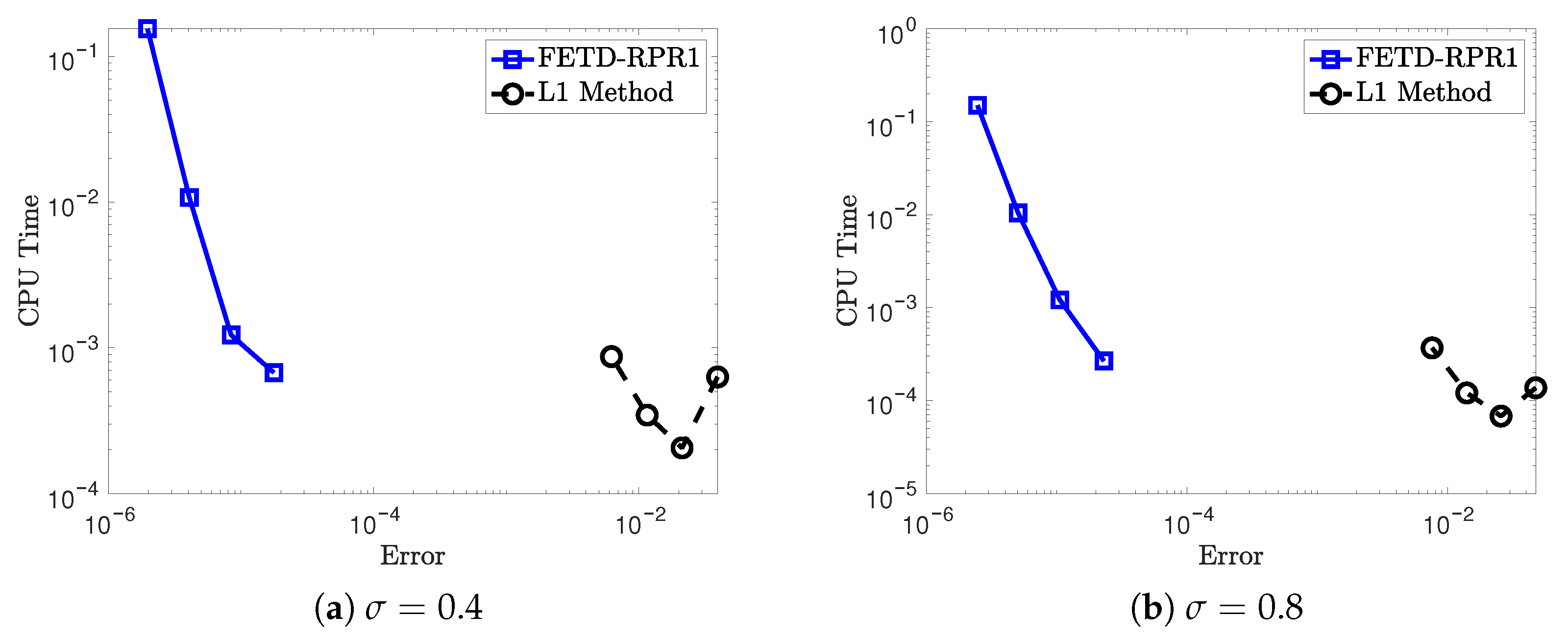
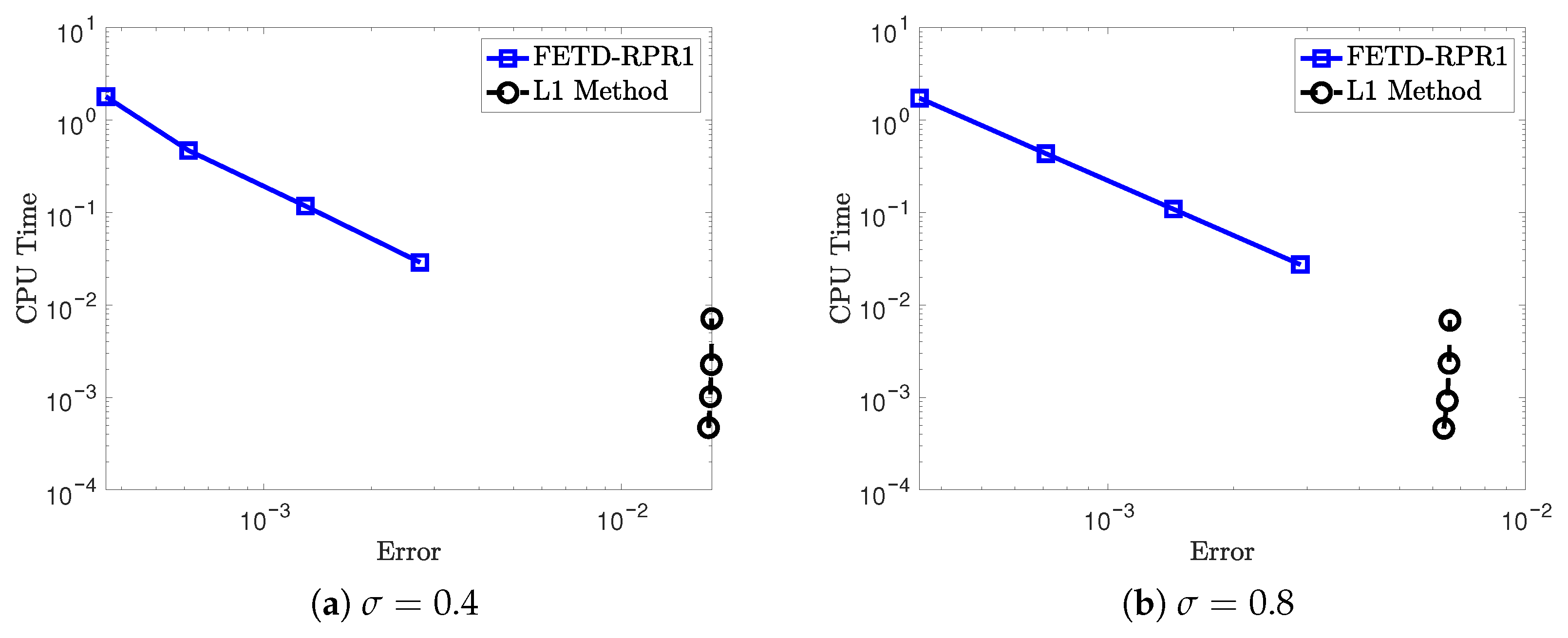
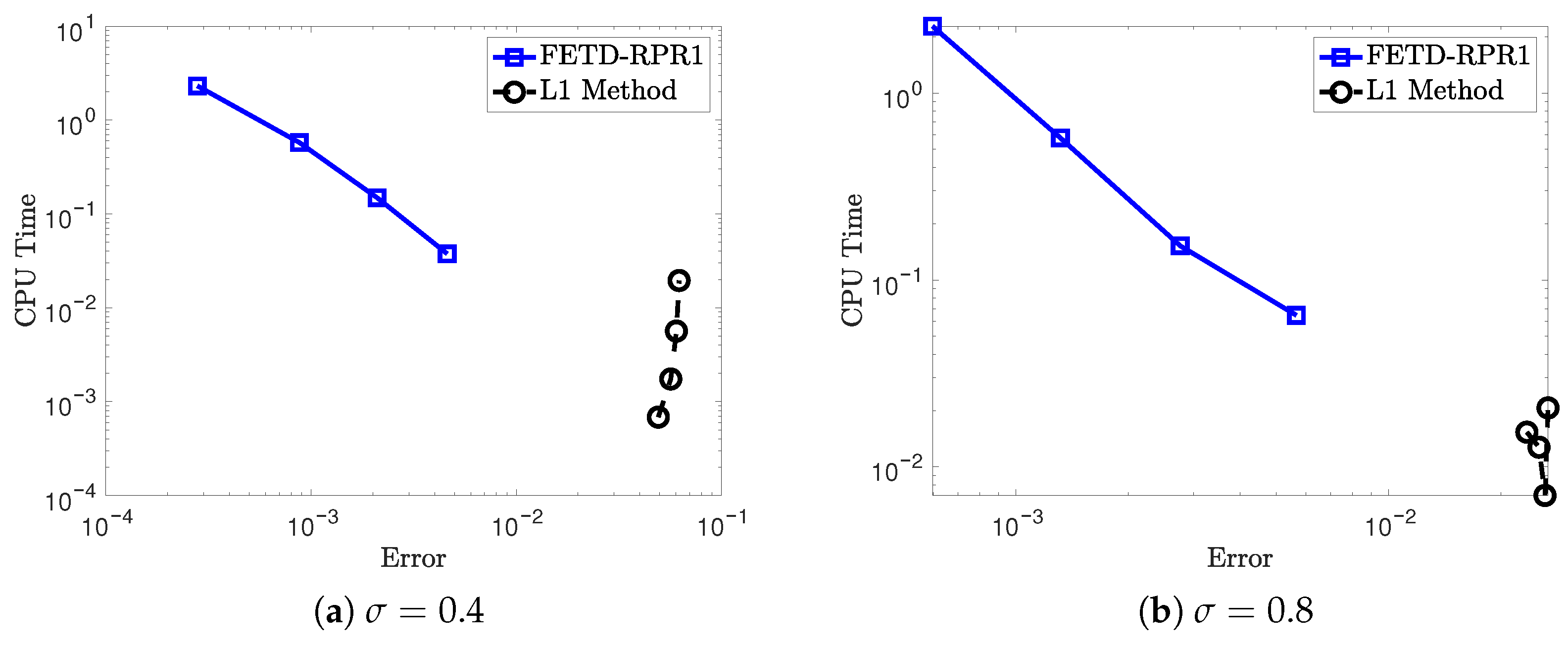
Using the same examples as presented in the previous subsection, we compare the L1 scheme in Algorithm 2 and the proposed FETD-RPR1 scheme. The comparison is made using the following parameters:

• Example 1: $\epsilon =2\times {10}^{-5}$, $k=0.1$, $M=40$.
• Example 3: $\epsilon =1.95\times {10}^{-5}$, $k=0.25$, $M=35$.
• Example 4: $\epsilon =9.89\times {10}^{-3}$, $k=0.02$, $M=35$.
• Example 5: ${\epsilon }_1=1.5\times {10}^{-5}$, ${\epsilon }_2=1.95\times {10}^{-3}$, $k=0.01$, $M=10$.
• Example 6: ${\epsilon }_1=3\times {10}^{-4}$, ${\epsilon }_2=9.1\times {10}^{-4}$, $k=0.01$, $M=20$.

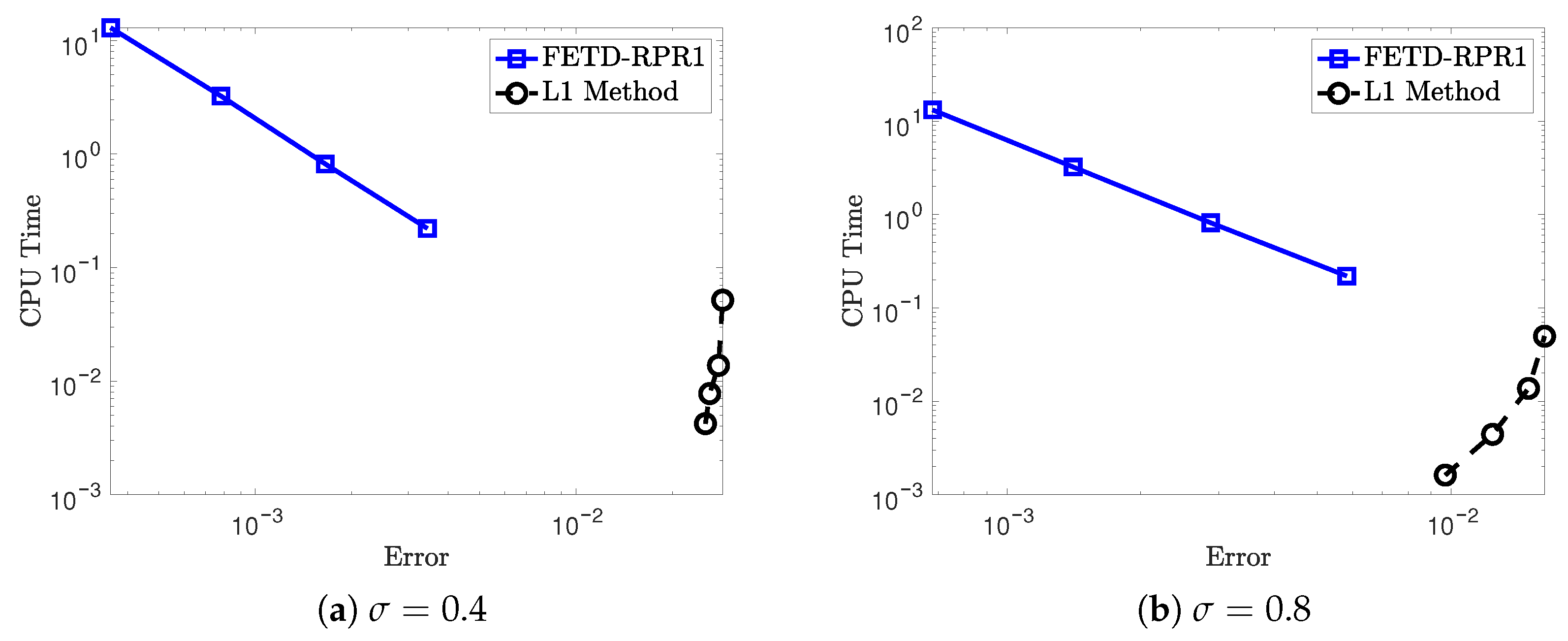
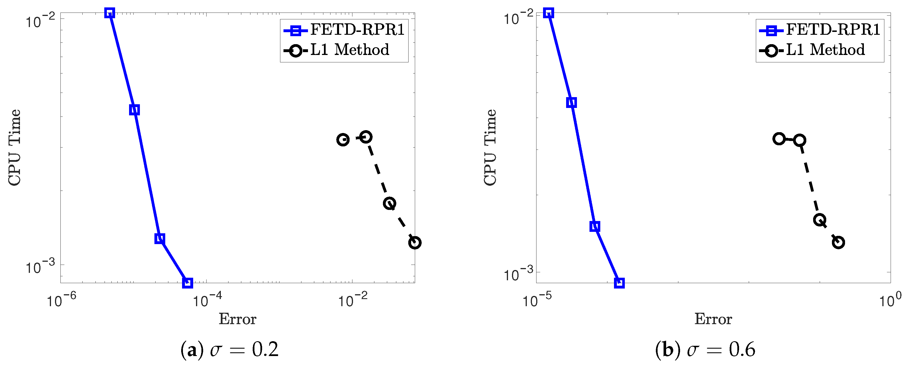
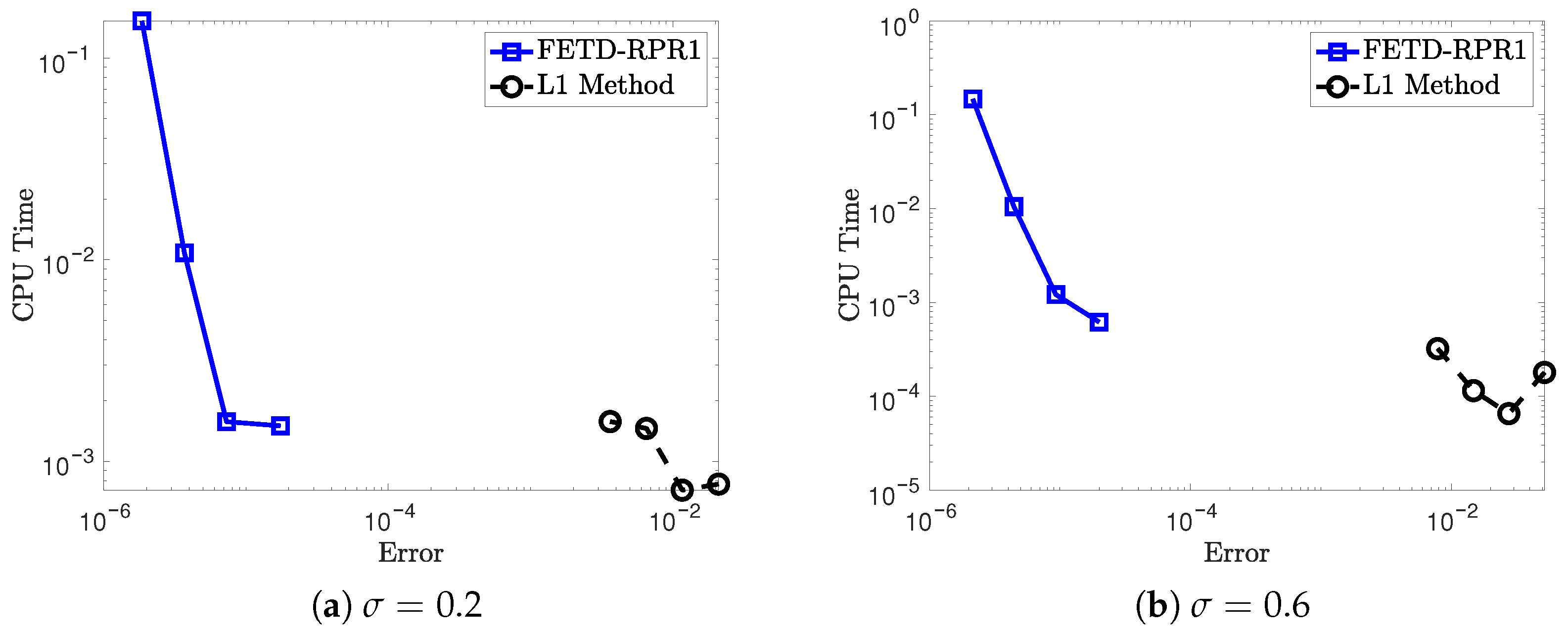
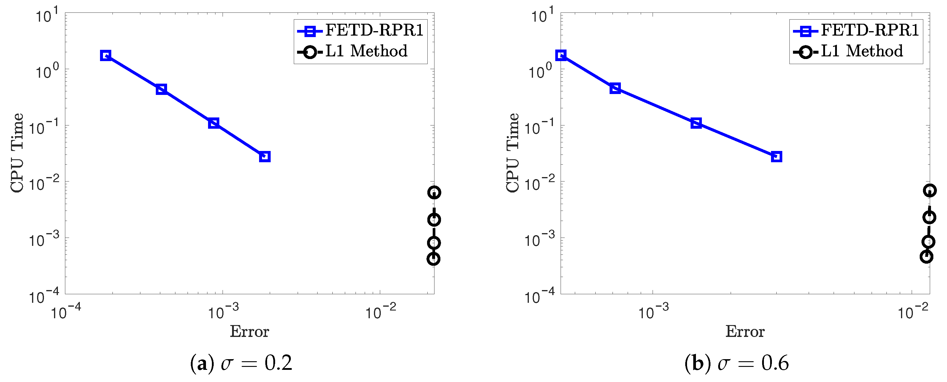
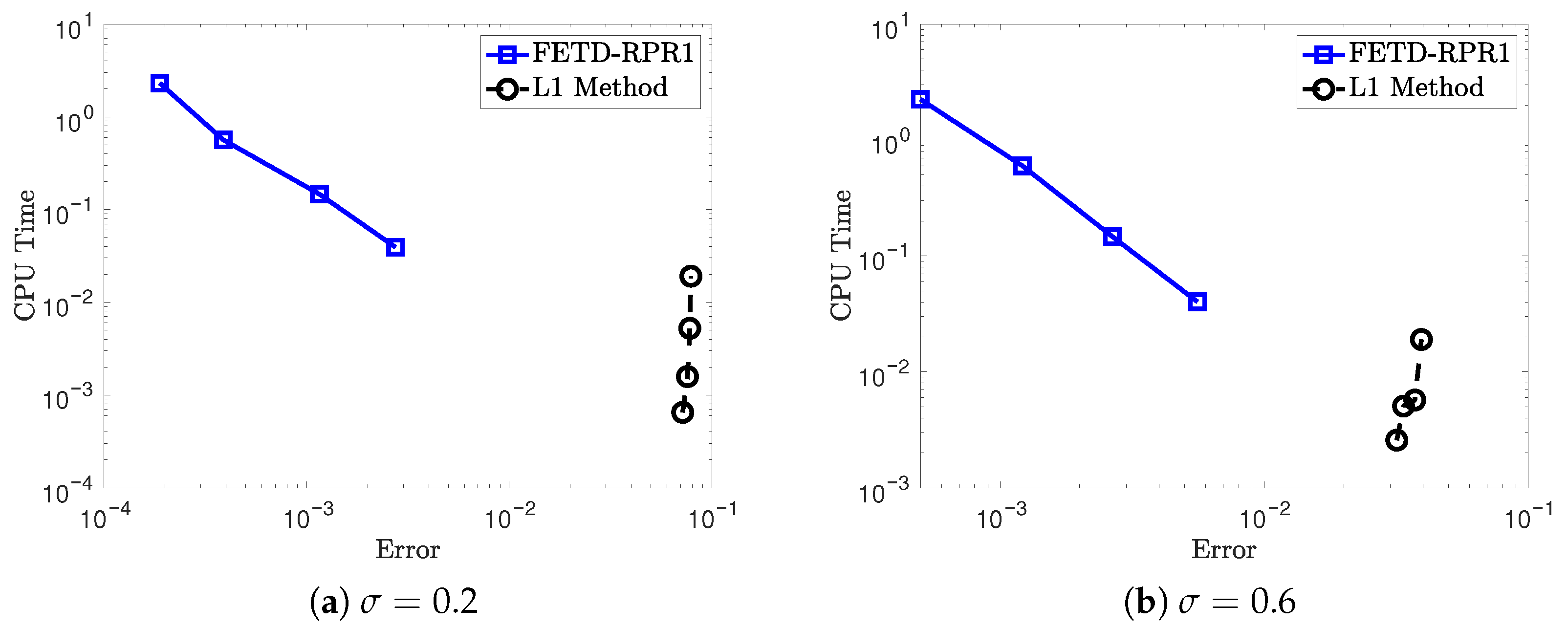
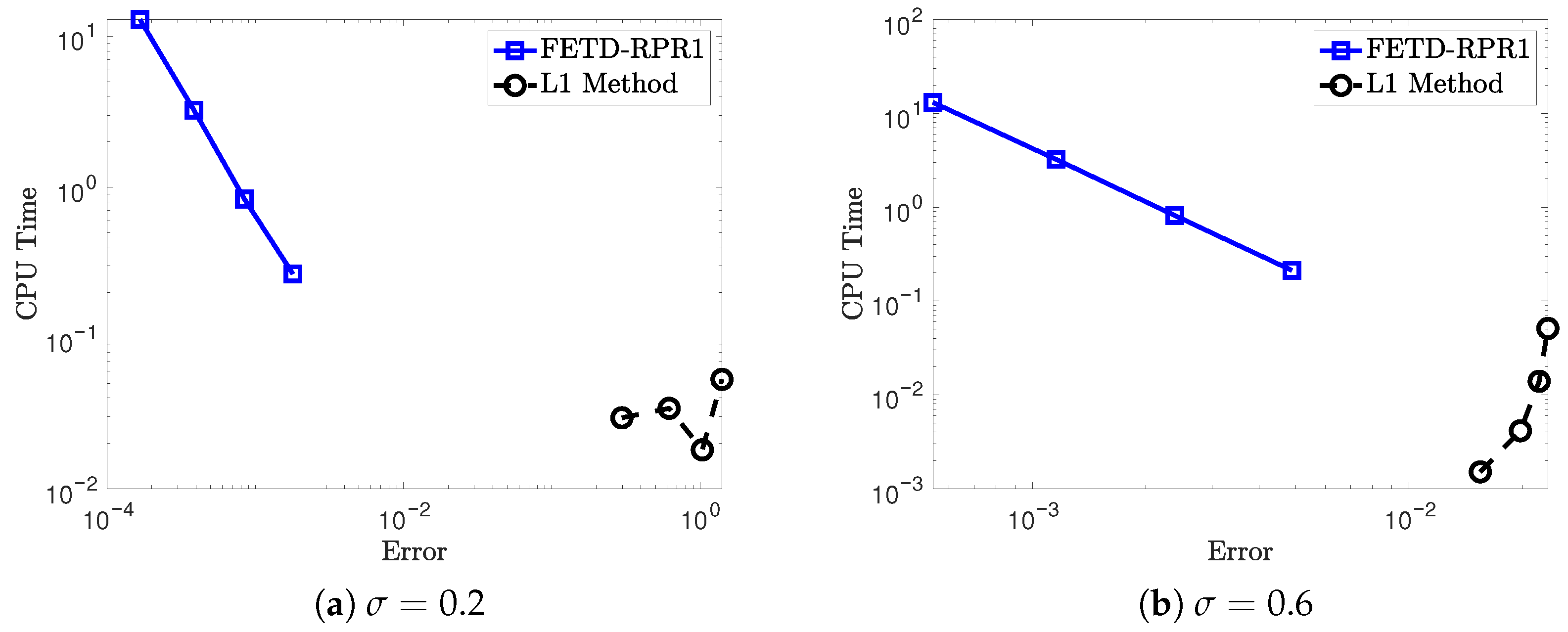
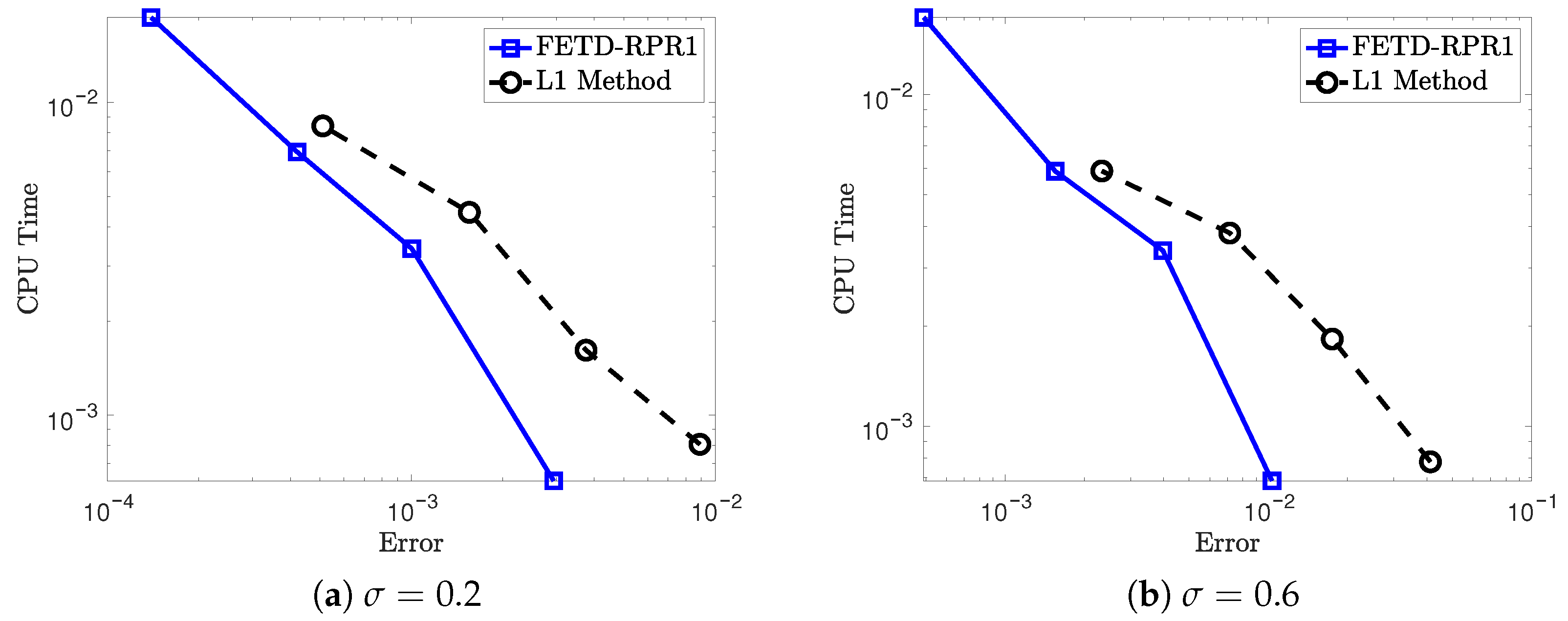
The results of the efficiency plots of the two methods are reported in Figure 41, Figure 42, Figure 43, Figure 44 and Figure 45.

As an application of the proposed scheme, we further investigate its efficiency and accuracy using the following Allen–Cahn equation whose exact solution does not exist.

Algorithm 2 L1 method

1: Define $k:$ time step, $M:$ number of spatial steps.    2: Compute ${\displaystyle h=\frac{b-a}{M}}$ with spatial domain $\mathrm{\Omega }=[a,b]$. Define $\sigma \in (0,1).$    3: Compute ${\displaystyle w_0=\frac{1}{\mathrm{\Gamma }(2-\sigma )}}$ and ${\displaystyle P=\frac{k^{\sigma }}{w_0}.}$    4: Set $n=1.$    5: Compute $a_n=W_i^{n-1},i=1,2,\dots ,M-1$ (Processor 1)    6: Solve for $b_n=\mathcal{H}(W_i^{n-1},t_{n-1})$ (Processor 2)    7: Solve for $c_n$ (Processor 3) $$\begin{array}{c}\hfill c_n={\displaystyle \frac{W_{i-1}^{n-1}-2W_i^{n-1}+W_{i+1}^{n-1}}{h^2}}.\end{array}$$    8: Solve for $d_n$ (Processor 4) $$\begin{array}{c}\hfill d_n={\displaystyle \sum _{k=0}^{n-1}}{w}_k^{\sigma }(W_i^{n-k}-W_i^{n-k-1}),\end{array}$$ where ${\displaystyle w_k^{\sigma }=\frac{{(k+1)}^{1-\sigma }-k^{1-\sigma }}{\mathrm{\Gamma }(2-\sigma )}.}$    9: Obtain approximate solution $W_i^n$ $$\begin{array}{c}\hfill {\displaystyle W_i^n=P(c_n+b_n)+a_n-\frac{1}{w_0}{d}_n.}\end{array}$$  10: set $n=n+1$. Go to step 5.

Example 7.

(1D time-fractional Allen–Cahn equation) Consider the following one-dimensional nonlinear Allen–Cahn problem:

$$\left\{\begin{array}{c}{}^{c}D^{\sigma }w=\lambda {\displaystyle \frac{{\partial }^{2}w}{\partial x^2}}+(w+x)-{(w+x)}^3,t\ge 0,x\in [-1,1],\hfill \\ w(x,0)=0.47\sin (-1.5\pi x)+0.53x-x,\hfill \\ w(0,t)=w(1,t)=0,\hfill \end{array}\right.$$

In

Table 7. Numerical results for Example 7.

			FETD-RPR1			L1 Method
$\mathit{\sigma }$	$\mathit{k}$	$\mathit{h}$	Error	OC	CPU Time	Error	OC	CPU Time
0.2	0.25000	0.2857	$2.9408\times {10}^{-3}$	-	$6.2000\times {10}^{-4}$	$8.9054\times {10}^{-3}$	-	$8.1000\times {10}^{-4}$
	0.12500	0.2857	$1.0035\times {10}^{-3}$	1.55	$3.4100\times {10}^{-3}$	$3.7574\times {10}^{-3}$	1.24	$1.6100\times {10}^{-3}$
	0.06250	0.2857	$4.2154\times {10}^{-4}$	1.25	$6.9400\times {10}^{-3}$	$1.5523\times {10}^{-3}$	1.28	$4.4500\times {10}^{-3}$
	0.03125	0.2857	$1.3932\times {10}^{-4}$	1.60	$1.8720\times {10}^{-2}$	$5.1133\times {10}^{-4}$	1.60	$8.4200\times {10}^{-3}$
0.4	0.25000	0.2857	$5.0145\times {10}^{-3}$	-	$9.0000\times {10}^{-4}$	$2.4579\times {10}^{-2}$	-	$7.4000\times {10}^{-4}$
	0.12500	0.2857	$2.1049\times {10}^{-3}$	1.25	$3.9900\times {10}^{-3}$	$9.4989\times {10}^{-3}$	1.37	$1.6900\times {10}^{-3}$
	0.06250	0.2857	$8.4579\times {10}^{-4}$	1.32	$7.1100\times {10}^{-3}$	$3.7799\times {10}^{-3}$	1.33	$4.3200\times {10}^{-3}$
	0.03125	0.2857	$2.6990\times {10}^{-4}$	1.65	$1.4440\times {10}^{-2}$	$1.2219\times {10}^{-3}$	1.63	$6.3100\times {10}^{-3}$
0.6	0.25000	0.2857	$1.0332\times {10}^{-2}$	-	$6.8000\times {10}^{-4}$	$4.1310\times {10}^{-2}$	-	$7.8000\times {10}^{-4}$
	0.12500	0.2857	$3.9787\times {10}^{-3}$	1.38	$3.3800\times {10}^{-3}$	$1.7497\times {10}^{-2}$	1.24	$1.8300\times {10}^{-3}$
	0.06250	0.2857	$1.5523\times {10}^{-3}$	1.36	$5.8800\times {10}^{-3}$	$7.1385\times {10}^{-3}$	1.29	$3.8200\times {10}^{-3}$
	0.03125	0.2857	$4.9071\times {10}^{-4}$	1.66	$1.7110\times {10}^{-2}$	$2.3311\times {10}^{-3}$	1.61	$5.8900\times {10}^{-3}$
0.8	0.25000	0.2857	$1.6158\times {10}^{-2}$	-	$6.5000\times {10}^{-4}$	$4.2453\times {10}^{-2}$	-	$7.8000\times {10}^{-4}$
	0.12500	0.2857	$6.5922\times {10}^{-3}$	1.29	$2.4400\times {10}^{-3}$	$2.0049\times {10}^{-2}$	1.08	$1.7400\times {10}^{-3}$
	0.06250	0.2857	$2.6305\times {10}^{-3}$	1.33	$7.1900\times {10}^{-3}$	$8.7630\times {10}^{-3}$	1.19	$4.1200\times {10}^{-3}$
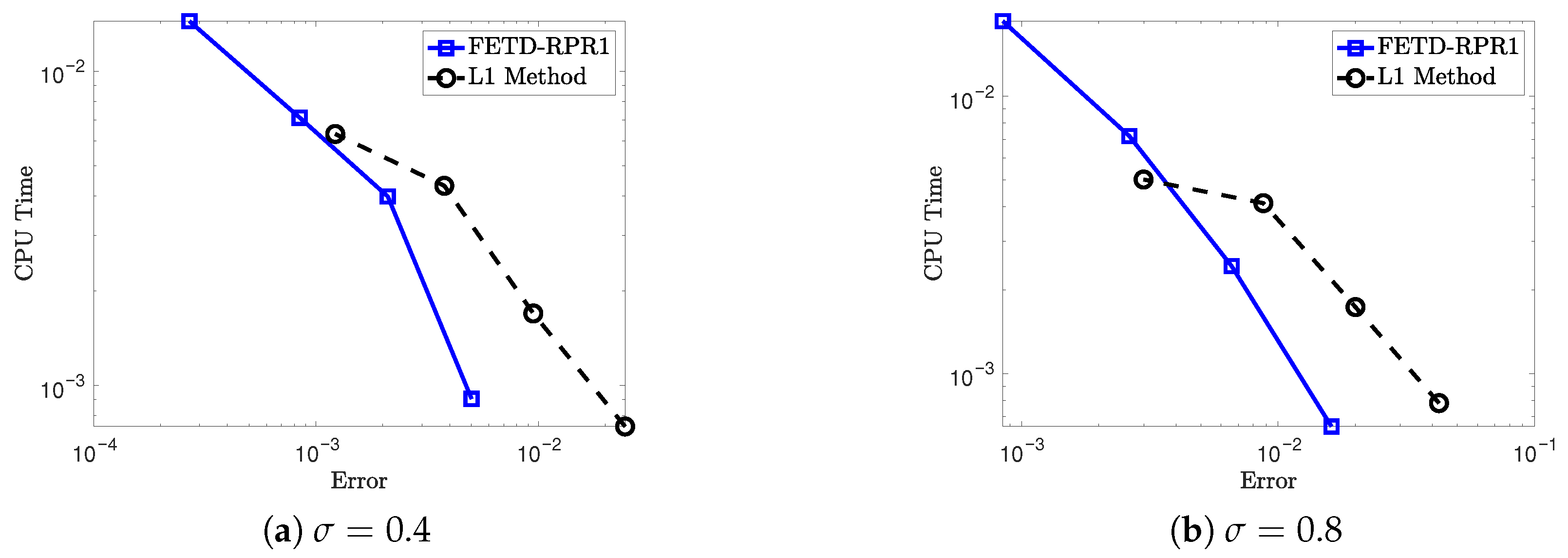
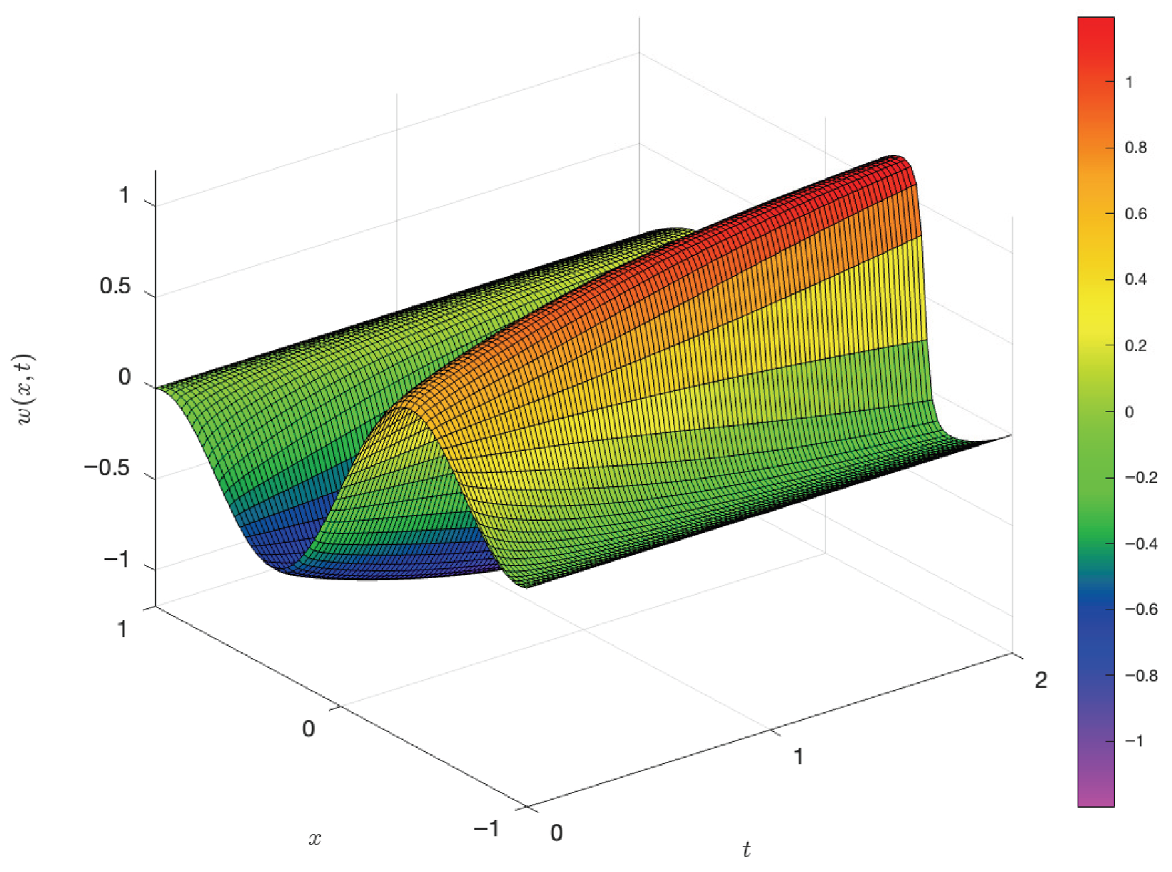
	0.03125	0.2857	$8.4401\times {10}^{-4}$	1.64	$1.8660\times {10}^{-2}$	$2.9883\times {10}^{-3}$	1.55	$5.0100\times {10}^{-3}$

, the errors, convergence order, and CPU time for the proposed scheme (FETD-RPR1) and the L1 method are detailed with grid refinement with parameters $\lambda =1\times {10}^{-3}$ for all $\sigma =0.2,0.4,0.6,0.8$. Since the exact solution does not exist for this problem, the numerical solutions using the corresponding scheme on a finer mesh are used as the reference solutions. It is clear that the proposed scheme attains a smaller norm error and shorter computational time compared to the L1 method. This efficiency and accuracy can be clearly observed in the convergence and efficiency plots in Figure 46 and Figure 47, respectively. To attain a certain significance of accuracy, the FETD-RPR1 method requires less computational time compared to the L1 method, which establishes the efficiency of the proposed method. The 3D solution plots in Figure 48 and Figure 49 were also observed when $\lambda =1\times {10}^{-4},k=0.02,h=0.02,T=2.$

Remark 3.

One of the major challenges in higher-order numerical schemes, specifically predictor–corrector-type algorithms for solving time-fractional models, is the need for more accurate and efficient lower-order predictors. Therefore, in this work, we try to address this challenge by developing a first-order numerical scheme which is robust in handling time-fractional models. However, the proposed first-order method needs the evaluation of the matrix vector product involving the Mittag-Leffler function. In numerical computation of this matrix vector product, the commonly used subroutine mlf leads to a significantly higher computational effort. To tackle this issue, we seek to have a more robust computationally effective numerical method to evaluate the Mittag-Leffler function involved in the matrix vector product in the proposed scheme. To that end, we developed a first-order rational approximation with a real pole (RPR1), which has been proven to be L-acceptable. The numerical experiment carried out in the comparison of the RPR1 approximation and the exact solution functions clearly states that RPR1 approximation is a good fit for MLF approximation, but with a limited application of asymptotic behavior for large arguments. Proving the theoretical convergence is another challenge, which motivated us to develop and prove a Grönwall-type inequality (as in Lemma 10) which we encountered in the main proof of Theorem 4. By employing the proposed RPR1 rational approximation of the matrix exponential, the method reduces the computational cost while maintaining stability. We empirically observed the accuracy and the efficiency of the proposed method (FETD-RPR1) with one-dimensional and two-dimensional (linear and nonlinear) examples and systems of time-fractional reaction–diffusion equations.

1. 

Figure 7, Figure 12, Figure 17, Figure 22, Figure 27, Figure 34 and Figure 46 establish the theoretical first-order convergence for all the examples in consideration in both linear and nonlinear time-fractional reaction–diffusion systems. Interestingly, the first-order convergence is observed for all values $\sigma =0.2,0.4,0.6,0.8$, which captures the range $\sigma \in (0,1).$

2. 

The proposed scheme is suitable for single-equation problems as well as coupled systems, making it versatile in practical applications.

3. 

Also, the proposed method demonstrates a lower error, which aligns with the exact solution in each example for all$\sigma =0.2,0.4,0.6,0.8.$ However, we noticed a significant increase in the error of variable u in solving Example 5, specifically when$\sigma =0.6,0.8.$

4. 

A comprehensive comparison of the proposed method with the L1 method consistently showed the efficiency of the FETD-RPR1 method. The better performance of the FETD-RPR1 method can be clearly seen from the efficiency plots in Figure 41, Figure 42, Figure 43, Figure 44, Figure 45 and Figure 47, which depict how the computational time behaved with respect to the error. In the efficiency plots, methods appearing further to the left demonstrated better computational efficiency.

5. 

It is clear that the FETD-RPR1 method is more computationally effective compared to the L1 method, although it requires the computation of matrix inverses.

6. 

It is interesting to notice that the proposed method (FETD-RPR1) attains almost close to a 1.6 order of convergence when it comes to solving complex problems which have no exact solution such as Example 7, which requires solving a time-fractional Allen–Cahn model.

7. 

The findings indicate that the proposed FETD-RPR1 method is a comparatively highly accurate and computationally efficient first-order method which can be employed as a predictor in second- and higher-order implicit numerical methods.

8. 

Although the proposed method is first-order in time and therefore offers lower temporal accuracy compared to higher-order schemes, this limitation is offset by its computational efficiency, accuracy, stability, and effectiveness as a reliable predictor in the development of higher-order methods.

7. Conclusions

In this study, we introduced a new L-acceptable, highly efficient numerical approximation for the Mittag-Leffler function (MLF) designed to mitigate spurious oscillations caused by non-smooth and mismatched initial and boundary conditions. This approach employs a rational function with a real pole to effectively evaluate the Mittag-Leffler function with matrix arguments. The Mittag-Leffler function is widely utilized and naturally emerges in numerical schemes for fractional models. Consequently, we propose a first-order explicit numerical method called the fractional exponential time differencing method with real pole rational approximation (FETD-RPR1) that leverages an efficient approximation of the Mittag-Leffler function using our proposed first-order real pole rational approximation (RPR1) to the Mittag-Leffler function. The performance of the scheme was evaluated for various fractional orders, namely, $\sigma =0.2,0.4,0.6,$ and $0.8$, using one-dimensional, two-dimensional, and systems of time-fractional reaction–diffusion problems, including both linear and nonlinear cases. The numerical results consistently demonstrate that the proposed method achieves good accuracy, with errors closely matching the exact solutions. In addition, its computational efficiency was assessed by comparing CPU time with that of the classical L1 method, showing a clear improvement. Furthermore, the strong performance of this explicit first-order scheme highlights its potential as a reliable predictor in the development of second- and higher-order implicit numerical methods, where an efficient and accurate initial approximation is essential.

References

1. Zubair, S.; Chaudhary, N.I.; Khan, Z.A.; Wang, W. Momentum fractional LMS for power signal parameter estimation. Signal Process. 2018, 142, 441–449. [Google Scholar] [CrossRef] [Scilit]
2. Albadarneh, R.B.; Batiha, I.; Alomari, A.K.; Tahat, N. Numerical approach for approximating the Caputo fractional-order derivative operator. AIMS Math. 2021, 6, 12743–12756. [Google Scholar] [CrossRef] [Scilit]
3. Tchier, F.; Inc, M.; Korpinar, Z.S.; Baleanu, D. Solutions of the time fractional reaction–diffusion equations with residual power series method. Adv. Mech. Eng. 2016, 8, 1687814016670867. [Google Scholar] [CrossRef] [Scilit]
4. Burrage, K.; Cardone, A.; D’Ambrosio, R.; Paternoster, B. Numerical solution of time fractional diffusion systems. Appl. Numer. Math. 2017, 116, 82–94. [Google Scholar] [CrossRef] [Scilit]
5. Iyiola, O.S.; Oduro, B.; Zabilowicz, T.; Iyiola, B.; Kenes, D. System of time fractional models for COVID-19: Modeling, analysis and solutions. Symmetry 2021, 13, 787. [Google Scholar] [CrossRef] [Scilit]
6. Iyiola, O.S.; Oduro, B.; Akinyemi, L. Analysis and solutions of generalized Chagas vectors re-infestation model of fractional order type. Chaos Solitons Fractals 2021, 145, 110797. [Google Scholar] [CrossRef] [Scilit]
7. Dwivedi, K.D.; Rajeev; Das, S.; Baleanu, D. Numerical solution of nonlinear space–time fractional-order advection–reaction–diffusion equation. J. Comput. Nonlinear Dynam. 2020, 15, 061005. [Google Scholar] [CrossRef] [Scilit]
8. Permyakova, E.V.; Goldobin, D.S. High-order schemes of exponential time differencing for stiff systems with nondiagonal linear part. J. Comput. Phys. 2025, 520, 113493. [Google Scholar] [CrossRef] [Scilit]
9. Wang, H.; Wang, K.; Sircar, T. A direct O(Nlog2N) finite difference method for fractional diffusion equations. J. Comput. Phys. 2010, 229, 8095–8104. [Google Scholar] [CrossRef] [Scilit]
10. Iyiola, O.S.; Wade, B.A. Exponential integrator methods for systems of non-linear space-fractional models with super-diffusion processes in pattern formation. Comput. Math. Appl. 2018, 75, 3719–3736. [Google Scholar]
11. Murio, D.A. Implicit finite difference approximation for time fractional diffusion equations. Comput. Math. Appl. 2008, 56, 1138–1145. [Google Scholar] [CrossRef] [Scilit]
12. Meerschaert, M.M.; Tadjeran, C. Finite difference approximations for two-sided space-fractional partial differential equations. Appl. Numer. Math. 2006, 56, 80–90. [Google Scholar] [CrossRef] [Scilit]
13. Meerschaert, M.M.; Tadjeran, C. Finite difference approximations for fractional advection–dispersion flow equations. J. Comput. Appl. Math. 2004, 172, 65–77. [Google Scholar] [CrossRef] [Scilit]
14. Deng, W. Finite element method for the space and time fractional Fokker–Planck equation. SIAM J. Numer. Anal. 2009, 47, 204–226. [Google Scholar] [CrossRef] [Scilit]
15. Liu, F.; Anh, V.; Turner, I. Numerical solution of the space fractional Fokker–Planck equation. J. Comput. Appl. Math. 2004, 166, 209–219. [Google Scholar] [CrossRef] [Scilit]
16. Baeumer, B.; Kovács, M.; Meerschaert, M.M. Numerical solutions for fractional reaction–diffusion equations. Comput. Math. Appl. 2008, 55, 2212–2226. [Google Scholar] [CrossRef] [Scilit]
17. Jafari, H.; Yousefi, S.A.; Firoozjaee, M.A.; Momani, S.; Khalique, C.M. Application of Legendre wavelets for solving fractional differential equations. Comput. Math. Appl. 2011, 62, 1038–1045. [Google Scholar] [CrossRef] [Scilit]
18. Yuanlu, L.I. Solving a nonlinear fractional differential equation using Chebyshev wavelets. Commun. Nonlinear Sci. Numer. Simul. 2010, 15, 2284–2292. [Google Scholar] [CrossRef] [Scilit]
19. Sweilam, N.H.; Nagy, A.M.; El-Sayed, A.A. On the numerical solution of space fractional order diffusion equation via shifted Chebyshev polynomials of the third kind. J. King Saud Univ. Sci. 2016, 28, 41–47. [Google Scholar] [CrossRef] [Scilit]
20. Iyiola, O.S.; Asante-Asamani, E.O.; Furati, K.M.; Khaliq, A.Q.M.; Wade, B.A. Efficient time discretization scheme for nonlinear space fractional reaction-diffusion equations. Int. J. Comput. Math. 2018, 95, 1274–1291. [Google Scholar] [CrossRef] [Scilit]
21. Chen, J.; Liu, F. Stability and convergence of an implicit difference approximation for the space Riesz fractional reaction-dispersion equation. Numer. Math. Engl. Ser. 2007, 16, 253. [Google Scholar]
22. Partohaghighi, M.; Asante-Asamani, E.; Iyiola, O.S. A robust numerical scheme for solving Riesz-tempered fractional reaction–diffusion equations. J. Comput. Appl. Math. 2024, 450, 115992. [Google Scholar] [CrossRef] [Scilit]
23. Li, H.L.; Hu, C.; Zhang, L.; Jiang, H.; Cao, J. Complete and finite-time synchronization of fractional-order fuzzy neural networks via nonlinear feedback control. Fuzzy Sets Syst. 2022, 443, 50–69. [Google Scholar] [CrossRef] [Scilit]
24. Li, H.L.; Hu, C.; Zhang, L.; Jiang, H.; Cao, J. Non-separation method-based robust finite-time synchronization of uncertain fractional-order quaternion-valued neural networks. Appl. Math. Comput. 2021, 409, 126377. [Google Scholar] [CrossRef] [Scilit]
25. Li, H.; Cao, J.; Hu, C.; Jiang, H.; Alsaadi, F.E. Synchronization Analysis of Discrete-Time Fractional-Order Quaternion-Valued Uncertain Neural Networks. IEEE Trans. Neural Netw. Learn. Syst. 2024, 35, 14178–14189. [Google Scholar] [CrossRef] [Scilit]
26. Pandey, P.; Kumar, S.; Gómez-Aguilar, J.F. Numerical solution of the time fractional reaction-advection-diffusion equation in porous media. J. Appl. Comput. Mech. 2022, 8, 84–96. [Google Scholar]
27. Afolabi, Y.O.; Biala, T.A.; Iyiola, O.S.; Khaliq, A.Q.; Wade, B.A. A Second-Order Crank-Nicolson-Type Scheme for Nonlinear Space–Time Reaction–Diffusion Equations on Time-Graded Meshes. Fract. Fractional. 2022, 7, 40. [Google Scholar] [CrossRef] [Scilit]
28. Sweilam, N.H.; Khader, M.M.; Mahdy, A.M.S. Crank-Nicolson finite difference method for solving time-fractional diffusion equation. J. Fract. Calc. Appl. 2012, 2, 1–9. [Google Scholar]
29. Garrappa, R. Exponential integrators for time–fractional partial differential equations. Eur. Phys. J. Spec. Top. 2013, 222, 1915–1927. [Google Scholar] [CrossRef] [Scilit]
30. Garrappa, R.; Popolizio, M. On accurate product integration rules for linear fractional differential equations. J. Comput. Appl. Math. 2011, 235, 1085–1097. [Google Scholar] [CrossRef] [Scilit]
31. Asante-Asamani, E.O.; Khaliq, A.Q.M.; Wade, B.A. A real distinct poles exponential time differencing scheme for reaction–diffusion systems. J. Comput. Appl. Math. 2016, 299, 24–34. [Google Scholar] [CrossRef] [Scilit]
32. Rasheed, S.; Iyiola, O.S.; Wade, B.A. A new second-order accurate strang splitting type exponential integrator for semilinear parabolic problems. Math. Comput. Simul. 2025, 240, 538–557. [Google Scholar] [CrossRef] [Scilit]
33. Asante-Asamani, E.O.; Kleefeld, A.; Wade, B.A. A second-order exponential time differencing scheme for non-linear reaction-diffusion systems with dimensional splitting. J. Comput. Phys. 2020, 415, 109490. [Google Scholar] [CrossRef] [Scilit]
34. Asante-Asamani, E.O. An Exponential Time Differencing Scheme with a Real Distinct Poles Rational Function for Advection-Diffusion Reaction Equations. Doctoral Dissertation, University of Wisconsin-Milwaukee, Milwaukee, WI, USA, 2016. [Google Scholar]
35. Cox, S.M.; Matthews, P.C. Exponential time differencing for stiff systems. J. Comput. Phys. 2002, 176, 430–455. [Google Scholar] [CrossRef] [Scilit]
36. Wiman, A. Über den Fundamentalsatz in der Teorie der Funktionen Eσ(x). Acta Math. 1905, 29, 191–201. [Google Scholar] [CrossRef] [Scilit]
37. Mittag-Leffler, G. Sur la nouvelle fonction Eσ(x). CR Acad. Sci. Paris 1903, 137, 554–558. [Google Scholar]
38. Garrappa, R. Numerical evaluation of two and three parameter Mittag-Leffler functions. SIAM J. Numer. Anal. 2015, 53, 1350–1369. [Google Scholar] [CrossRef] [Scilit]
39. Diethelm, K.; Ford, N.J.; Freed, A.D.; Luchko, Y. Algorithms for the fractional calculus: A selection of numerical methods. Comput. Methods Appl. Mech. Eng. 2005, 194, 743–773. [Google Scholar] [CrossRef] [Scilit]
40. Atkinson, C.; Osseiran, A. Rational solutions for the time-fractional diffusion equation. SIAM J. Appl. Math. 2011, 7, 92–106. [Google Scholar] [CrossRef] [Scilit]
41. Zeng, C.; Chen, Y.Q. Global Padé approximations of the generalized Mittag-Leffler function and its inverse. Fract. Calc. Appl. Anal. 2015, 18, 1492–1506. [Google Scholar] [CrossRef] [Scilit]
42. Iyiola, O.S.; Asante-Asamani, E.O.; Wade, B.A. A real distinct poles rational approximation of generalized Mittag–Leffler functions and their inverses: Applications to fractional calculus. J. Comput. Appl. Math. 2018, 330, 307–317. [Google Scholar] [CrossRef] [Scilit]
43. Sarumi, I.O.; Furati, K.M.; Khaliq, A.Q.M. Highly accurate global Padé approximations of generalized Mittag–Leffler function and its inverse. J. Sci. Comput. 2018, 82, 46. [Google Scholar] [CrossRef] [Scilit]
44. Garra, R.; Gorenflo, R.; Polito, F.; Tomovski, Ž. Hilfer–Prabhakar derivatives and some applications. Appl. Math. Comput. 2014, 242, 576–589. [Google Scholar] [CrossRef] [Scilit]
45. Ray, S.S. Exact solutions for time-fractional diffusion-wave equations by decomposition method. Phys. Scr. 2006, 75, 53. [Google Scholar] [CrossRef] [Scilit]
46. Karbalaie, A.; Montazeri, M.M.; Muhammed, H.H. New approach to find the exact solution of fractional partial differential equation. WSEAS Trans. Math. 2012, 11, 908–917. [Google Scholar]
47. Sharma, U.P.; Agarwal, R.; Nisar, K.S. Bicomplex two-parameter Mittag-Leffler function and properties with application to the fractional time wave equation. Palest. J. Math. 2023, 12, 456. [Google Scholar]
48. Podlubny, I. Fractional Differential Equations: Mathematics in Science and Engineering; Academic Press Inc.: San Diego, CA, USA, 1998; Volume 198. [Google Scholar]
49. Garrappa, R.; Popolizio, M. Generalized exponential time differencing methods for fractional order problems. Comput. Math. Appl. 2011, 62, 876–890. [Google Scholar] [CrossRef] [Scilit]
50. Haubold, H.J.; Mathai, A.M.; Saxena, R.K. Mittag-Leffler functions and their applications. J. Appl. Math. 2011, 2011, 298628. [Google Scholar] [CrossRef] [Scilit]
51. Pang, D.; Jiang, W.; Niazi, A.U. Fractional derivatives of the generalized Mittag-Leffler functions. Adv. Differ. Equ. 2018, 2018, 415. [Google Scholar] [CrossRef] [Scilit]
52. Apelblat, A. Differentiation of the Mittag-Leffler functions with respect to parameters in the Laplace transform approach. Mathematics 2020, 85, 657. [Google Scholar] [CrossRef] [Scilit]
53. Dixon, J. On the order of the error in discretization methods for weakly singular second kind non-smooth solutions. BIT Numer. Math. 1985, 25, 623–634. [Google Scholar] [CrossRef] [Scilit]
54. Stynes, M. A survey of the L1 scheme in the discretisation of time-fractional problem. Numer. Math. Theory Methods Appl. 2022, 15, 1173–1192. [Google Scholar] [CrossRef] [Scilit]
55. Yang, Z.; Zeng, F. A corrected L1 method for a time-fractional subdiffusion equation. J. Sci. Comput. 2023, 95, 85. [Google Scholar] [CrossRef] [Scilit]
Figure 1. RPR1 approx. for f 1 ( w ) .
Axioms 15 00288 g001
Figure 2. RPR1 approx. for f 2 ( w ) .
Axioms 15 00288 g002
Figure 3. RPR1 approx. for f 3 ( w ) .
Axioms 15 00288 g003
Figure 4. RPR1 approx. for f 4 ( w ) .
Axioms 15 00288 g004
Figure 5. RPR1 approx. for f 5 ( w ) .
Axioms 15 00288 g005
Figure 6. RPR1 approx. for f 6 ( w ) .
Axioms 15 00288 g006
Figure 7. Convergence plots for Example 1.
Axioms 15 00288 g007
Figure 8. Example 1 solution at T = 2 : σ = 0.4 .
Axioms 15 00288 g008
Figure 9. Example 1 solution at T = 2 : σ = 0.8 .
Axioms 15 00288 g009
Figure 10. Example 1 exact solution: σ = 0.6 .
Axioms 15 00288 g010
Figure 11. Example 1 FETD-RPR1: σ = 0.6 .
Axioms 15 00288 g011
Figure 12. Convergence plots for Example 2.
Axioms 15 00288 g012
Figure 13. Example 2 exact solution: σ = 0.6 .
Axioms 15 00288 g013
Figure 14. Example 2 FETD-RPR1: σ = 0.6 .
Axioms 15 00288 g014
Figure 15. Example 2 solution profile: σ = 0.4 .
Axioms 15 00288 g015
Figure 16. Example 2 solution profile: σ = 0.8 .
Axioms 15 00288 g016
Figure 17. Convergence plots for Example 3.
Axioms 15 00288 g017
Figure 18. Example 3 solution at T = 1 : σ = 0.4 .
Axioms 15 00288 g018
Figure 19. Example 3 solution at T = 1 : σ = 0.8 .
Axioms 15 00288 g019
Figure 20. Example 3 exact solution: σ = 0.6 .
Axioms 15 00288 g020
Figure 21. Example 3 FETD-RPR1: σ = 0.6 .
Axioms 15 00288 g021
Figure 22. Convergence plots for Example 4.
Axioms 15 00288 g022
Figure 23. Example 4 solution at T = 1 : σ = 0.4 .
Axioms 15 00288 g023
Figure 24. Example 4 solution at T = 1 : σ = 0.8 .
Axioms 15 00288 g024
Figure 25. Example 4 exact solution: σ = 0.6 .
Axioms 15 00288 g025
Figure 26. Example 4 FETD-RPR1: σ = 0.6 .
Axioms 15 00288 g026
Figure 27. Convergence plots for Example 5.
Axioms 15 00288 g027
Figure 28. Example 5 solution u: T = 1 , σ = 0.6 .
Axioms 15 00288 g028
Figure 29. Example 5 solution v: T = 1 , σ = 0.6 .
Axioms 15 00288 g029
Figure 30. Example 5 exact solution u: σ = 0.6 .
Axioms 15 00288 g030
Figure 31. Example 5 FETD-RPR1 solution u: σ = 0.6 .
Axioms 15 00288 g031
Figure 32. Example 5 exact solution v: σ = 0.6 .
Axioms 15 00288 g032
Figure 33. Example 5 FETD-RPR1 solution v: σ = 0.6 .
Axioms 15 00288 g033
Figure 34. Convergence plots for Example 6.
Axioms 15 00288 g034
Figure 35. Example 6 solution u: T = 1 , σ = 0.6 .
Axioms 15 00288 g035
Figure 36. Example 6 solution v: T = 1 , σ = 0.6 .
Axioms 15 00288 g036
Figure 37. Example 6 exact solution u: σ = 0.6 .
Axioms 15 00288 g037
Figure 38. Example 6 FETD-RPR1 solution u: σ = 0.6 .
Axioms 15 00288 g038
Figure 39. Example 6 exact solution v: σ = 0.6 .
Axioms 15 00288 g039
Figure 40. Example 6 FETD-RPR1 solution of v: σ = 0.6 .
Axioms 15 00288 g040
Figure 41. Efficiency plots for Example 1: FETD-RPR1 vs. L1 method.
Axioms 15 00288 g041
Figure 42. Efficiency plots for Example 3: FETD-RPR1 vs. L1 method.
Axioms 15 00288 g042
Figure 43. Efficiency plots for Example 4: FETD-RPR1 vs. L1 method.
Axioms 15 00288 g043
Figure 44. Efficiency plots for Example 5: FETD-RPR1 vs. L1 method.
Axioms 15 00288 g044
Figure 45. Efficiency plots for Example 6: FETD-RPR1 vs. L1 method.
Axioms 15 00288 g045
Figure 46. Convergence plots for Example 7: FETD-RPR1 vs. L1 method.
Axioms 15 00288 g046
Figure 47. Efficiency plots for Example 7: FETD-RPR1 vs. L1 method.
Axioms 15 00288 g047
Figure 48. Example 7 FETD-RPR1 solution: σ = 0.6 .
Axioms 15 00288 g048
Figure 49. Example 7 L1 method solution: σ = 0.6 .
Axioms 15 00288 g049