Abstract
In this paper, we initiate the study of the asymptotic and oscillatory properties of solutions to third-order functional differential equations. Using the Riccati transformation to eliminate the existence of non-oscillatory solutions, we derive various oscillation criteria that address different models of the studied equation. Our primary focus is on reducing the constraints imposed on oscillation criteria, thereby broadening their applicability. Our results improve, refine, and extend some of the known findings in previous studies. Several examples are presented to illustrate the significance of the main results.
MSC:
34C10; 22E70; 34K11
1. Introduction
This paper deals with the oscillatory behavior of solutions to a third-order neutral delay differential equation of the form
for where is a quotient of two odd positive integers and We assume the following assumptions:
- (I1)
- and
- (I2)
- ,and
- (I3)
- , and Furthermore, does not vanish eventually.
Definition 1.
A solution of (1) is defined as for a certain with the corresponding function
where and y satisfies (1) on and
Furthermore, if a solution y of (1) has arbitrarily large zeros, it is considered oscillatory; otherwise, it is called a non-oscillatory solution.
Definition 2.
Oscillation theory and computing are closely linked, especially in solving complex differential equations and dynamic systems. Computational methods inspired by oscillation theory help to analyze the stability and behavior of solutions, particularly in periodic or aperiodic systems. With advances in computing, oscillatory patterns in high-dimensional or nonlinear systems can be efficiently modelled. This connection broadens the practical applications of oscillation theory in areas such as signal processing and control systems [1].
The study of oscillatory behavior in differential equations represents a fundamental area of mathematical research, owing to its wide-ranging applications in physics, engineering, and biology. Oscillation theory focuses on identifying the conditions under which solutions to differential equations exhibit oscillatory behavior, thereby providing valuable insights into their qualitative characteristics. Within this framework, third-order differential equations have received considerable attention, as they serve as effective models for complex dynamical systems, including beam vibrations in mechanics, electrical circuits, and control processes. These equations commonly arise in higher-order systems, where second-order descriptions fall short of capturing the intricate dynamics. A general third-order linear differential equation can be expressed as
where and are real-valued coefficient functions. Oscillation theory focuses on understanding the zeros of , the points at which , and determining the nature and frequency of these zeros.
Numerical methods are essential for solving complex differential equations, particularly when analytical solutions are unavailable. These methods approximate solutions by discretising and solving systems of linear and nonlinear equations iteratively, using techniques like finite differences, finite elements, Runge-Kutta methods, and spectral methods plus (preconditioned) Krylov solvers. For oscillatory differential equations, specialized algorithms, such as time-stepping approaches and Fourier transforms, are used to capture periodic behavior and identify frequency components. These methods are crucial in systems where oscillations are central, including mechanical vibrations, electrical circuits, and population dynamics. We refer the reader to [2,3,4,5,6] and references therein for concrete algorithms and the related computational costs also from the perspective of associated numerical linear algebra issues.
Oscillatory solutions are those with infinitely many zeros as , while non-oscillatory solutions have at most a finite number of zeros. The study of oscillation for third-order differential equations is particularly challenging due to the interplay between the coefficients and higher derivative terms. Unlike second-order equations, where Sturm’s comparison and separation theorems provide a robust framework, third-order equations often require the development of new methodologies and criteria. Various techniques, including comparison principles, integral averaging, Riccati equations, and Lyapunov functional approaches, have been adapted and extended for the analysis of these equations [7,8,9,10,11,12,13].
In the literature, oscillation criteria have been established for both linear and nonlinear third-order differential equations. Significant progress has been made in studying equations with variable coefficients, delay terms, and forced oscillations. Researchers have developed sufficient conditions for oscillation based on integral inequalities, properties of associated functions, and the asymptotic behavior of coefficients. The motivation for studying the oscillation of third-order differential equations comes from their practical applications and theoretical implications, see [14,15,16,17,18,19,20]. In engineering, they describe stability and resonance phenomena in mechanical and electrical systems. In physics, they model the propagation of waves and the stability of structures. Moreover, in pure mathematics, they contribute to the broader understanding of dynamical systems and spectral theory.
The study of oscillatory behavior in differential equations benefits from the structural insights of Lie algebra. Lie symmetries provide a systematic method for analyzing differential systems. They reveal invariant transformations under which the equations preserve their form. By doing so, these symmetries can simplify complex systems, reduce their dimensionality, or even yield exact solutions. In oscillatory dynamics, the underlying Lie algebraic structures play a key role. They can describe conserved quantities, periodic orbits, and integrability conditions. Identifying the Lie algebra associated with a system also enables classification of its oscillatory regimes. It further provides a deeper geometric understanding of the phase space. This interplay between oscillatory analysis and Lie theory forms a powerful framework. It uncovers hidden patterns and supports the analytical treatment of dynamical systems that would otherwise be intractable [21,22].
In the past decade, significant progress has been achieved in the development of oscillation theory for third-order delay differential equations (see, e.g., [23,24,25,26]). Specifically, the authors in [15,27,28] developed oscillation criteria for nonlinear differential equation of the form
by comparing it to first-order oscillatory differential equations.
Elabbasy et al. in [13] extended the oscillation criteria established by [15,27] to a more general third-order delay differential equation of the form
which applies to both cases:
Wang, Meng, and Gu [29] investigated the following third-order neutral differential equations with damping and distributed deviating arguments:
where they established new oscillation criteria using a refined generalized Riccati transformation and integral averaging techniques. Their results extend previous results.
Tian, Cai, Fu, and Li [30] explored third-order neutral differential equations with distributed deviating arguments:
where and . Using a generalized Riccati transformation and integral averaging techniques, they obtained Philos-type criteria that ensuring every solution is either oscillatory or converges to zero.
Sun and Zhao [31] examined third-order neutral delay differential equations with distributed deviating arguments:
where
for and and established new oscillatory criteria.
Baculikova and Dzurina [8], Candan in [19,32] established different oscillation criteria for the equation
under the condition
In [33], the authors studied the oscillation of solutions to equation
under the condition (5). On the other hand, Han et al. [34] considered the oscillation for third-order neutral differential equation
where
Karpuz et al. [35] investigated the oscillation of odd-order delay differential equations of the form
under the condition
This work presents new insights into the oscillatory behavior of third-order differential equation solutions. It extends classical results and employs advanced techniques to establish refined oscillation criteria for a broader class of equations. These results enrich the theoretical framework of oscillation theory and provide valuable tools for applications across diverse scientific fields.
Lemma 1
([35]). Let , , and satisfies and for all further, assume that there is a function where such that
for all Suppose that exists and Then leads to
Lemma 2
([36]). Let . Then
where
2. Main Results
Here, we suppose the following conditions:
or
The following lemma will play a useful role in the subsequent results:
Lemma 3.
Proof.
Let be a solution of (1). We can prove the case for , as follows a similar approach. According to (2), we note that and
That is, and has one sign. Moreover, is a positive and has one sign. Also, either or for . We claim that . If not, then there is a constant such that
Integrating (15) from to ⊤, we have
Thus,
Then, using and , we see that , that is, . Now, suppose that . From (1), we have
From (2) and by using Lemma 2, we obtain
Using (12) and (17) in (16), we have
Integrating (18) from ⊤ to ∞, we get
Using and (14), we have
That is
According Lemma 1, we note that
and in view of (10), and since , we get
In (19), we see that
Integrating from ⊤ to ∞, we obtain
Integrating (20) from to ∞, we get
this contradicts (11). Thus is positive. Hence, the proof is established. □
Lemma 4.
Proof.
According the fact that is nonincreasing. Then we have
Also,
This completes the proof. □
In the following subsections, we will suppose that there exists a function for
2.1. Oscillation Criteria When (8) Holds
Proof.
Let be a solution of (1). As in the proof of Lemma 3, we get (13) and (18). Thus, by using Lemma 4, we obtain (21). Now, define the following function:
That is, according to Lemma 3, , and
In view of (13), (21) and we find
Using (24) and (25), we get
Define another function as follows:
That is, according to Lemma 3, , and
Taking (13) and (21) with the fact that into account, we have
which from (27) and (28) implies that
Using (26) and (29), we obtain
By (18) and (30), we obtain
By applying the inequality stated in [37], namely,
we see that
and
Substituting (33) and (34) into (31), we are led to
Integrating above inequality from to ⊤, we see that
Hence, the proof is established. □
By Lemma 2, and using a similar approach to the proof of Theorem 1, we derive the subsequent result.
Theorem 2.
Theorem 3.
Proof.
Let be a solution of (1), which does not asymptotically approach zero. As in the proof of Lemma 3, we get (13) and (18). By using Lemma 4, we have (21) and (22).
Using the definition of both functions and v by (24) and (27), respectively. Similarly as in the proof of Theorem 1, we get (25) and (28), which from (25) yields
According to (13), (21), (22) and , we have
Using (39) in (38), and in view (25), we get
Now, from (28), we see that
Using (13), (21), (22) and , we are led to
Combining (42) and (41), and applying (28), we obtain
By (40) and (43), we get
By applying the inequality stated in [37], namely,
we see that
and
Substituting (45) and (46) into (44), we obtain
Integrating (47) from to ⊤, we have
and contradicts (37). The proof is complete. □
From Lemma 2, and following a similar approach to the proof of Theorem 3, we obtain the following result.
2.2. Oscillation Criteria When (9) Holds
Proof.
Let be a solution of (1), which does not asymptotically approach zero. As proof of Lemma 3, we get (13) and (18). That is, by Lemma 4, we obtain (21). Define the positive function
It follows that
Using (13), (21) and we have
With the use of (50) and (51), we deduce
Now, define the following positive function
That is,
From (13) and (21), we have
which from (53) and (54) implies
Using (52) and (55), we have
By (13), (18), (56) and we obtain
Using (57) and (32), we get
Integrating (58) from to ⊤, we have
which is a contradiction (49). With the latter the proof is complete. □
Using Lemma 2 and proceeding as in the proof of Theorem 5, we obtain the following theorem.
Theorem 6.
Using (51), (54), and applying a similar approach to the proof of Theorem 3, we obtain the following theorem.
In view of Lemma 2 and Theorem 7, similar to the proof of Theorem 3, we get the following result.
Remark 1.
Based on Theorems 1–8, we can derive oscillation criteria of (1) for various choices of ℏ.
2.3. Philos-Type Oscillation Criteria
In this section, we will derive Philos-type oscillation results for (1). Suppose that and Let be an element of we say that the function has property P if it satisfies the following assumptions:
- (I)
- (II)
- has a continuous partial derivative with respect to the second variable in , which is non-positive.
2.3.1. Philos-Type Criteria When (8) Holds
Theorem 9.
Proof.
According to Theorem 2, similar to the proof of Theorem 9, we obtain the following theorem.
Theorem 10.
Theorem 11.
From Theorem 4, as in the proof of Theorem 9, we obtain the following result.
Theorem 12.
By (57) in Theorem 5, as in the proof of Theorem 9, we conclude the following result.
2.3.2. Philos-Type Criteria When (9) Holds
Theorem 13.
By Theorem 6, as in the proof of Theorem 9, we conclude the following theorem.
Theorem 14.
By Theorem 7, as in the proof of Theorem 9, we get the following result.
Theorem 15.
By Theorem 8, as in the proof of that of Theorem 9, we obtain the following theorem.
Theorem 16.
Remark 2.
Using Theorems 9–16, we can derive oscillation criteria of (1) for various choices of ℏ and Γ.
3. Examples
Example 1.
Consider the equation
where Here, and . Set
Remark 3.
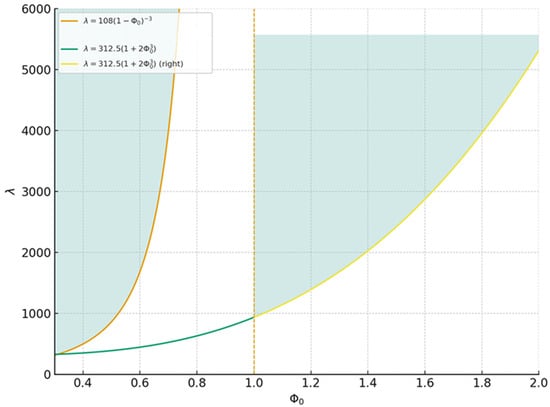
In Figure 1, Example 1 demonstrates a clear superiority over the results of the study in [8], and this can be discussed as follows:
Figure 1.
Test of the strength of criteria for Equation (74).
- 1.
- 2.
- The results in [8] were restricted to the interval . Consequently, this results fails to provide any oscillation results once reaches or exceeds unity. In contrast, our formulation remains valid up to (green area enclosed during in Figure 1), where the cubic condition dominates and ensures the existence of feasible solutions. This extended validity represents a clear improvement and demonstrates the robustness of our approach.
Example 2.
Remark 4.
For Example 2, we note that:
- 1.
- At we (78) impliesIn view of ([8], Example 1), it is found that the result is obtained as a necessary condition for (77) to has property N was as followsBy comparing results (80) and (81), we find thatThus, our results improve results of [8].
- 2.
- Figure 2 illustrates a direct comparison between Theorem 1 (solid yellow curve) and Theorem 3 (dashed blue curve). It is evident that Theorem 1 consistently provides smaller values of λ across the examined range of , reflecting a tighter and more efficient bound. In contrast, Theorem 3 grows significantly faster. That is Theorem 1 offers a stronger and more reliable characterization of the oscillatory condition.
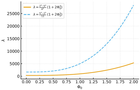 Figure 2. Test of the strength of criteria for Equation (77).

Example 3.
Remark 5.
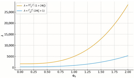
In Figure 3, the results clearly indicate that Theorem 5 (blue curve) yields consistently smaller values of λ across the entire range of . This reflects a tighter and more efficient bound compared to Theorem 7 (yellow curve), whose rapid growth demonstrates weaker control. Thus, for Example 3, we see that Theorem 5 is better than Theorem 7.
Figure 3.
Test of the strength of criteria for Equation (82).
4. Conclusions
In this work, we examine the oscillatory behavior of solutions to Equation (1). Our results extend and refine previous research by relaxing the conditions placed on the functions involved in the equation. Specifically, we introduce the condition , in contrast to the more restrictive conditions (5)–(7) that were commonly applied in earlier studies, such as those in [8,19,32,33,34,35]. These previous conditions fail in models where the function falls outside the range Our proofs rely on various forms of Riccati assumptions, which allow us to derive results applicable to a broad spectrum of models. Furthermore, we investigate the oscillatory behavior of Equation (1) when the condition (9) holds (see Theorems 9–16).
This work presents a novel analysis of the general Equation (1), which, to the best of our knowledge, has not been addressed in previous studies. The approach we take enables the inclusion of a wider range of models, setting our work apart from earlier research and offering new directions for further investigation.
Future studies could extend this work by examining the oscillatory behavior of (1) in the case where the function is oscillatory. Additionally, the methodology developed in this paper can be adapted to analyze more generalized equations in the form
where
In addition to the sufficient conditions established in this work and the detailed analysis we have provided, a natural extension of the present study would be to investigate whether these conditions are close to being necessary. Such an extension would further strengthen the theoretical framework and provide a sharper characterization of the parameter space.
Finally, based on the oscillation criteria examined in this study, it is evident that under Riccati’s assumptions, the solutions maintain a crucial property of boundedness. This ensures that they neither diverge nor exhibit instability over time. By linking oscillatory behavior with stability, we confirm that the solutions remain well-behaved within finite bounds, further supporting the notion of stability in dynamic systems. Thus, the interplay between oscillation and stability offers significant insights into the long-term behavior and boundedness of the system under consideration. In this direction, we emphasize that there is a lot of work to do and we leave it for future investigations.
Author Contributions
Conceptualization, A.A.-J., E.A. and B.Q.; methodology, A.A.-J., B.Q. and E.A.; validation, A.A.-J., B.Q. and E.A.; investigation, A.A.-J. and B.Q.; resources, B.Q. and A.A.-J.; data curation, A.A.-J. and B.Q.; writing—original draft preparation, A.A.-J., E.A. and B.Q.; writing—review and editing, B.Q., A.A.-J., S.S.-C. and E.A.; visualization, A.A.-J., E.A., S.S.-C. and B.Q.; supervision, A.A.-J., S.S.-C., E.A. and B.Q.; project administration, B.Q. All authors have read and agreed to the published version of the manuscript.
Funding
This research was funded by Researchers Supporting Project number (PNURSP2025R406), Princess Nourah Bint Abdulrahman University, Riyadh, Saudi Arabia.
Data Availability Statement
Data are contained within the article.
Acknowledgments
Authors would like to thank Princess Nourah bint Abdulrahman University Researchers Supporting Project number (PNURSP2025R406), Princess Nourah bint Abdulrahman University, Riyadh, Saudi Arabia.
Conflicts of Interest
The authors declare no conflicts of interest.
References
- Krasnosel’skii, M.A.; Pokrovskii, A.V. Systems with Hysteresis; Springer Science & Business Media: New York, NY, USA, 2012. [Google Scholar]
- Al-Jaser, A.; Qaraad, B.; Ramos, H.; Serra-Capizzano, S. New Conditions for Testing the Oscillation of Solutions of Second-Order Nonlinear Differential Equations with Damped Term. Axioms 2024, 13, 105. [Google Scholar] [CrossRef]
- Linders, V.; Birken, P. Locally conservative and flux consistent iterative methods. SIAM J. Sci. Comput. 2024, 46, S424–S444. [Google Scholar] [CrossRef]
- Dravins, I.; Serra-Capizzano, S.; Neytcheva, M. Spectral Analysis of Preconditioned Matrices Arising from Stage-Parallel Implicit Runge–Kutta Methods of Arbitrarily High Order. SIAM J. Matrix Anal. Appl. 2024, 45, 1007–1034. [Google Scholar] [CrossRef]
- McDonald, E.; Pestana, J.; Wathen, A. Preconditioning and iterative solution of all-at-once systems for evolutionary partial differential equations. SIAM J. Sci. Comput. 2018, 40, A1012–A1033. [Google Scholar] [CrossRef]
- Ferrari, P.; Furci, I.; Hon, S.; Ayman-Mursaleen, M.; Serra-Capizzano, S. The eigenvalue distribution of special 2-by-2 block matrix-sequences with applications to the case of symmetrized Toeplitz structures. SIAM J. Matrix Anal. Appl. 2019, 40, 1066–1086. [Google Scholar] [CrossRef]
- Hale, J.K. Theory of Functional Differential Equations; Springer: New York, NY, USA, 1977. [Google Scholar] [CrossRef]
- Baculíková, B.; Džurina, J. Oscillation of third-order neutral differential equations. Math. Comput. Model. 2010, 52, 215–226. [Google Scholar] [CrossRef]
- Džurina, J.; Grace, S.R.; Jadlovská, I. On nonexistence of Kneser solutions of third-order neutral delay differential equations. Appl. Math. Lett. 2019, 88, 193–200. [Google Scholar] [CrossRef]
- Thandapani, E.; Tamilvanan, S.; Jambulingam, E.; Tech, V.T.M. Oscillation of third order half-linear neutral delay differential equations. Int. J. Pure Appl. Math. 2012, 77, 359–368. [Google Scholar]
- Jiang, Y.; Li, T. Asymptotic behavior of a third-order nonlinear neutral delay differential equation. J. Inequal. Appl. 2014, 2014, 512. [Google Scholar] [CrossRef]
- Tunc, E. Oscillatory and asymptotic behavior of third-order neutral differential equations with distributed deviating arguments. Electron. J. Differ. Equ. 2017, 2017, 1–12. Available online: https://ejde.math.txstate.edu/Volumes/2017/16/tunc.pdf (accessed on 10 November 2025). [CrossRef]
- Elabbasy, E.M.; Hassan, T.; Elmatary, B.M. Oscillation criteria for third order delay nonlinear differential equations. Electron. J. Qual. Theory Differ. Equ. 2012, 2012, 1–9. [Google Scholar] [CrossRef]
- Graef, J.R.; Tunc, E.; Grace, S.R. Oscillatory and asymptotic behavior of a third-order nonlinear neutral differential equation. Opusc. Math. 2017, 37, 839–852. [Google Scholar] [CrossRef]
- Grace, S.R.; Agarwal, R.P.; Pavani, R.; Thandapani, E. On the oscillation of certain third-order nonlinear functional differential equations. Appl. Math. Comput. 2008, 202, 102–112. [Google Scholar] [CrossRef]
- Džurina, J.; Thandapani, E.; Tamilvanan, S. Oscillation of solutions to third-order half-linear neutral differential equations. Electron. J. Differ. Equ. 2012, 2012, 1–9. [Google Scholar]
- Li, T.; Zhang, C.; Xing, G. Oscillation of third-order neutral delay differential equations. In Abstract and Applied Analysis; Hindawi: London, UK, 2012; Volume 2012, p. 569201. [Google Scholar] [CrossRef]
- Li, T.; Rogovchenko, Y.V. On asymptotic behavior of solutions to higher-order sublinear emden–fowler delay differential equations. Appl. Math. Lett. 2017, 67, 53–59. [Google Scholar] [CrossRef]
- Candan, T. Asymptotic properties of solutions of third-order nonlinear neutral dynamic equations. Adv. Differ. Equ. 2014, 2014, 35. [Google Scholar] [CrossRef]
- Philos, C.G. On the existence of nonoscillatory solutions tending to zero at ∞ for differential equations with positive delays. Arch. Math. 1981, 36, 168–178. [Google Scholar] [CrossRef]
- Hall, B.C. Lie Groups, Lie Algebras, and Representations. In Quantum Theory for Mathematicians. Graduate Texts in Mathematics; Springer: New York, NY, USA, 2013; Volume 267, pp. 333–366. [Google Scholar] [CrossRef]
- Knapp, A.W. Lie Groups Beyond an Introduction; Birkhäuser: Boston, MA, USA, 1996; Volume 140. [Google Scholar] [CrossRef]
- Jadlovská, I.; Chatzarakis, G.E.; Džurina, J.; Grace, S.R. On Sharp Oscillation Criteria for General Third-Order Delay Differential Equations. Mathematics 2021, 9, 1675. [Google Scholar] [CrossRef]
- Graef, J.R.; Jadlovská, I.; Tunç, E. Sharp asymptotic results for third-order linear delay differential equations. J. Appl. Anal. Comput. 2021, 11, 2459–2472. [Google Scholar] [CrossRef]
- Grace, S.R. Oscillation criteria for third order nonlinear delay differential equations with damping. Opuscula Math. 2015, 35, 485–497. [Google Scholar] [CrossRef]
- Baculíková, B.; Džurina, J. Oscillation of the third order Euler differential equation with delay. Math. Bohem. 2014, 139, 649–655. [Google Scholar] [CrossRef]
- Baculíková, B.; Džurina, J. Oscillation of third-order nonlinear differential equations. Appl. Math. Lett. 2011, 24, 466–470. [Google Scholar] [CrossRef]
- Saker, S.H.; Džurina, J. On the oscillation of certain class of third-order nonlinear delay differential equations. Math. Bohem. 2010, 135, 225–237. [Google Scholar] [CrossRef]
- Wang, Y.; Meng, F.; Gu, J. Oscillation criteria of third-order neutral differential equations with damping and distributed deviating arguments. Adv. Differ. Equ. 2021, 2021, 515. [Google Scholar] [CrossRef]
- Tian, Y.; Cai, Y.; Fu, Y.; Li, T. Oscillation and asymptotic behavior of third-order neutral differential equations with distributed deviating arguments. Adv. Differ. Equ. 2015, 2015, 267. Available online: https://advancesincontinuousanddiscretemodels.springeropen.com/articles/10.1186/s13662-015-0604-6 (accessed on 10 November 2025). [CrossRef]
- Sun, Y.; Zhao, Y. Oscillatory behavior of third-order neutral delay differential equations with distributed deviating arguments. J. Inequal. Appl. 2019, 2019, 207. [Google Scholar] [CrossRef]
- Candan, T. Oscillation criteria and asymptotic properties of solutions of third-order nonlinear neutral differential equations. Math. Methods Appl. Sci. 2014, 38, 1379–1392. [Google Scholar] [CrossRef]
- Zhong, J.; Ouyang, Z.; Zou, S. Oscillation criteria for a class of third-order nonlinear neutral differential equations. J. Appl. Anal. 2011, 17, 155–163. [Google Scholar] [CrossRef]
- Han, Z.; Li, T.; Zhang, C.; Sun, S. An oscillation criterion for third-order neutral delay differential equations. J. Appl. Anal. 2010, 16, 295–303. [Google Scholar] [CrossRef]
- Karpuz, B.; Öcalan, Ö.; Öztürk, S. Comparison theorems on the oscillation and asymptotic behavior of higher-order neutral differential equations. Glasgow Math. J. 2010, 52, 107–114. [Google Scholar] [CrossRef]
- Thandapani, E.; Li, T. On the oscillation of third-order quasi-linear neutral functional differential equations. Arch. Math. 2011, 47, 181–199. [Google Scholar]
- Zhang, S.; Wang, Q. Oscillation of second-order nonlinear neutral dynamic equations on times cales. Appl. Math. Comput. 2010, 216, 2837–2848. [Google Scholar] [CrossRef]
Disclaimer/Publisher’s Note: The statements, opinions and data contained in all publications are solely those of the individual author(s) and contributor(s) and not of MDPI and/or the editor(s). MDPI and/or the editor(s) disclaim responsibility for any injury to people or property resulting from any ideas, methods, instructions or products referred to in the content. |
© 2025 by the authors. Licensee MDPI, Basel, Switzerland. This article is an open access article distributed under the terms and conditions of the Creative Commons Attribution (CC BY) license (https://creativecommons.org/licenses/by/4.0/).