Deferred Cesàro Summability and Korovkin-Type Approximation Theorems for Double Sequences on Time Scales

Abstract

This paper investigates fundamental concepts of statistical convergence for double sequences of time-scale functions via the deferred Cesàro summability mean. Several limit properties and inclusion relations between the newly-introduced convergence notions are established. Based on these concepts, a number of Korovkin-type approximation theorems are proved for time-scale functions of two variables by using suitable algebraic test functions. Illustrative examples involving a positive linear operator associated with bivariate Bernstein polynomials are presented to demonstrate the applicability of the theoretical results. In addition, the rate of statistical convergence with respect to the deferred Cesàro summability method is studied and estimated.

1. Introduction

The concept of statistical convergence was first introduced by Zygmund [1] in 1935. Later, Fast [2] and Steinhaus [3] independently developed this notion in the framework of sequence space theory. In the year 1980, Salát [4] systematically studied the fundamental properties of statistically convergent sequences of real numbers. Subsequently, Fridy [5,6] further investigated the basic notions and limit properties of statistical convergence for real-valued sequences.

In the context of approximation theory, Mohiuddine et al. [7] introduced the concept of statistical summability $(C,1)$ and established a Korovkin-type approximation theorem. In recent years, statistical convergence and summability methods have attracted significant attention due to their wide applicability in approximation theory and integration theory. Srivastava et al. [8] introduced a class of weighted statistical convergence and proved Korovkin-type approximation theorems using trigonometric test functions. Subsequently, Srivastava et al. [9] developed the notion of statistical integrability for sequences of functions and established Korovkin-type approximation results for statistically Riemann- and Lebesgue-integrable sequences.

The study of double sequences was initiated in this context by Srivastava et al. [10], who established new classes of Korovkin-type approximation theorems. More recently, statistical gauge integrability and its applications to approximation theory have been investigated in [11], including results for functions of two variables. Furthermore, fuzzy approximation theorems based on statistical deferred Nörlund summability were obtained in [12], highlighting the versatility and wide applicability of statistical summability methods in diverse functional settings. Some other recent contributions to approximation theory employing statistical convergence can be found in [11,12].

A time scale is defined as any nonempty closed subset of the real line and is commonly denoted by $\mathbb{T}$. In this work, we endow $\mathbb{T}$ with the topology induced from the usual topology on $\mathbb{R}$. The theory of time-scale calculus was originally developed by Stefan Hilger in his doctoral dissertation in 1988 under the supervision of B. Aulbach (see [13,14]). This framework was designed to provide a unified treatment of continuous and discrete analysis within a single mathematical setting. By allowing functions to be defined on an arbitrary time scale, one may study dynamical phenomena that exhibit both continuous and discrete behavior in a systematic way. Time-scale calculus has found numerous applications, particularly in the study of dynamic equations and their qualitative properties [15]. The notion of statistical convergence in the continuous setting was first examined by Mòricz [16]. Later, Guseinov [17] introduced the concepts of Riemann $\Delta$- and ∇-integrals on time scales and explored their fundamental properties. Since then, a substantial body of literature has emerged devoted to the development and applications of time-scale calculus; see, for example, refs. [14,18,19,20,21,22] and the references cited therein.

Motivated by the above-mentioned investigations, we first introduce the basic concepts of statistical convergence for double sequences of time-scale functions via the deferred Cesàro summability mean. Several important limit properties and inclusion relations among these newly introduced types of convergence are discussed. Based on these notions, Korovkin-type approximation theorems are established for time-scale functions of two variables using suitable algebraic test functions. To illustrate the theoretical results, an example involving a positive linear operator associated with Bernstein polynomials in two variables is presented. Furthermore, the rate of statistical convergence with respect to the deferred Cesàro summability method is studied and estimated.

2. A Set of Preliminaries

Let ${\sigma }_1:{\mathbb{T}}_1\to {\mathbb{T}}_1$ and ${\sigma }_2:{\mathbb{T}}_2\to {\mathbb{T}}_2$ be the forward jump operators defined by

$$\begin{array}{c}\hfill {\sigma }_1\left(t_1\right)=inf\{r_1\in {\mathbb{T}}_1:r_1>t_1\}\end{array}$$

and

$$\begin{array}{c}\hfill {\sigma }_2\left(t_2\right)=inf\{r_2\in {\mathbb{T}}_2:r_2>t_2\}\end{array}$$

for all $t_1\in {\mathbb{T}}_1$ and $t_2\in {\mathbb{T}}_2$.

Similarly, let ${\rho }_1:{\mathbb{T}}_1\to {\mathbb{T}}_1$ and ${\rho }_2:{\mathbb{T}}_2\to {\mathbb{T}}_2$ be the backward jump operators defined by

$$\begin{array}{c}\hfill {\rho }_1\left(t_1\right)=sup\{r_1\in {\mathbb{T}}_1:r_1<t_1\}\end{array}$$

and

$$\begin{array}{c}\hfill {\rho }_2\left(t_2\right)=sup\{r_2\in {\mathbb{T}}_2:r_2<t_2\}\end{array}$$

for all $t_1\in {\mathbb{T}}_1$ and $t_2\in {\mathbb{T}}_2$.

The graininess functions ${\mu }_1:{\mathbb{T}}_1\to [0,\infty )$ and ${\mu }_2:{\mathbb{T}}_2\to [0,\infty )$ are defined by

$$\begin{array}{c}\hfill {\mu }_1\left(t_1\right)={\sigma }_1\left(t_1\right)-t_1\end{array}$$

and

$$\begin{array}{c}\hfill {\mu }_2\left(t_2\right)={\sigma }_2\left(t_2\right)-t_2\end{array}$$

for all $(t_1,t_2)\in {\mathbb{T}}_1\times {\mathbb{T}}_2.$

Here we set $inf⌀=sup{\mathbb{T}}_i$ (that is, ${\sigma }_i\left(t_i\right)=t_i$ if ${\mathbb{T}}_i$ has a maximum $t_i$) and $sup⌀=inf{\mathbb{T}}_i$ (that is, ${\rho }_i\left(t_i\right)=t_i$ if ${\mathbb{T}}_i$ has a minimum $t_i$) for $i=1,2$, where ⌀ denotes the empty set.

A closed interval, open interval, and semi-closed (or semi-open) interval on the time-scale product ${\mathbb{T}}^2={\mathbb{T}}_1\times {\mathbb{T}}_2$ are defined, respectively, by

$$\begin{array}{c}\hfill {[a_1,b_1]}_{{\mathbb{T}}_1}\times {[a_2,b_2]}_{{\mathbb{T}}_2}=\{(t_1,t_2)\in {\mathbb{T}}_1\times {\mathbb{T}}_2:a_1\leqq t_1\leqq b_1,a_2\leqq t_2\leqq b_2\},\end{array}$$

$$\begin{array}{c}\hfill {(a_1,b_1)}_{{\mathbb{T}}_1}\times {(a_2,b_2)}_{{\mathbb{T}}_2}=\{(t_1,t_2)\in {\mathbb{T}}_1\times {\mathbb{T}}_2:a_1<t_1<b_1,a_2<t_2<b_2\}\end{array}$$

and

$$\begin{array}{c}\hfill {[a_1,b_1)}_{{\mathbb{T}}_1}\times {[a_2,b_2)}_{{\mathbb{T}}_2}=\{(t_1,t_2)\in {\mathbb{T}}_1\times {\mathbb{T}}_2:a_1\leqq t_1<b_1,a_2\leqq t_2<b_2\}\end{array}$$

for all $a_i,b_i\in \mathbb{R}$$(i=1,2)$.

Now, let $\mathcal{A}$ denote the family of all left-closed and right-open rectangles on ${\mathbb{T}}^2$ of the form:

$$\begin{array}{c}\hfill {[a_1,b_1)}_{{\mathbb{T}}_1}\times {[a_2,b_2)}_{{\mathbb{T}}_2}.\end{array}$$

Also let $S:\mathcal{A}\to [0,\infty )$ be the set function on $\mathcal{A}$ defined by

$$\begin{array}{c}\hfill S\left({[a_1,b_1)}_{{\mathbb{T}}_1}\times {[a_2,b_2)}_{{\mathbb{T}}_2}\right)=(b_1-a_1)(b_2-a_2),\end{array}$$

where S is a countably additive measure on $\mathcal{A}$.

The Carathéodory extension of the set function S defined on the algebra $\mathcal{A}$ gives rise to a measure on ${\mathbb{T}}^2$, which is referred to as the Lebesgue $\Delta$-measure and is denoted by ${\mu }_{\Delta }$. This measure provides a natural framework for integrating functions defined on time-scale products ${\mathbb{T}}^2={\mathbb{T}}_1\times {\mathbb{T}}_2$.

A real-valued function $g:{\mathbb{T}}^2\to \mathbb{R}$ is said to be $\Delta$-measurable if, for every open set $A\subset \mathbb{R}$, the preimage

$$\begin{array}{c}\hfill g^{-1}\left(A\right)=\{(t_1,t_2)\in {\mathbb{T}}_1\times {\mathbb{T}}_2:g(t_1,t_2)\in A\}\end{array}$$

belongs to the $\sigma$-algebra generated by the Lebesgue $\Delta$-measure. This notion of measurability ensures that standard measure-theoretic tools can be applied to functions defined on ${\mathbb{T}}^2$ within the time-scale setting.

Definition 1.

For each $(a_1,a_2)\in {\mathbb{T}}^2\setminus max\left\{{\mathbb{T}}^2\right\},$ the singleton point set $\left\{(a_1,a_2)\right\}$ is Δ-measurable, and its Δ-measure is given by

$$\begin{array}{c}\hfill {\mu }_{\Delta }(a_1,a_2)={\mu }_{{\Delta }_1}\left(a_1\right){\mu }_{{\Delta }_2}\left(a_2\right)=\left({\sigma }_1\left(a_1\right)-a_1\right)\left({\sigma }_2\left(a_2\right)-a_2\right).\end{array}$$

Theorem 1.

Let $(a_1,a_2),(b_1,b_2)\in {\mathbb{T}}^2$ with $a_i\leqq b_i$$(i=1,2)$. Then

$$\begin{array}{c}\hfill {\mu }_{\Delta }\left({(a_1,b_1)}_{{\mathbb{T}}_1}\times {(a_2,b_2)}_{{\mathbb{T}}_2}\right)=\left(b_1-{\sigma }_1\left(a_1\right)\right)\left(b_2-{\sigma }_2\left(a_2\right)\right)\end{array}$$

and

$$\begin{array}{c}\hfill {\mu }_{\Delta }\left({[a_1,b_1)}_{{\mathbb{T}}_1}\times {[a_2,b_2)}_{{\mathbb{T}}_2}\right)=(b_1-a_1)(b_2-a_2).\end{array}$$

Moreover, if $(a_1,a_2),(b_1,b_2)\in {\mathbb{T}}^2\setminus max\left\{{\mathbb{T}}^2\right\}$ with $a_i\leqq b_i$ for $i=1,2,$ then

$$\begin{array}{c}\hfill {\mu }_{\Delta }\left({(a_1,b_1]}_{{\mathbb{T}}_1}\times {(a_2,b_2]}_{{\mathbb{T}}_2}\right)=\left({\sigma }_1\left(b_1\right)-{\sigma }_1\left(a_1\right)\right)\left({\sigma }_2\left(b_2\right)-{\sigma }_2\left(a_2\right)\right)\end{array}$$

and

$$\begin{array}{c}\hfill {\mu }_{\Delta }\left({[a_1,b_1]}_{{\mathbb{T}}_1}\times {[a_2,b_2]}_{{\mathbb{T}}_2}\right)=\left({\sigma }_1\left(b_1\right)-a_1\right)\left({\sigma }_2\left(b_2\right)-a_2\right).\end{array}$$

Proof. 

Let ${\mathbb{T}}_1$ and ${\mathbb{T}}_2$ be two time scales and let ${\mathbb{T}}^2={\mathbb{T}}_1\times {\mathbb{T}}_2$. The Lebesgue $\Delta$-measure ${\mu }_{\Delta }$ on ${\mathbb{T}}^2$ is defined as the Carathéodory extension of the set function:

$$\begin{array}{c}\hfill S\left({[a_1,b_1)}_{{\mathbb{T}}_1}\times {[a_2,b_2)}_{{\mathbb{T}}_2}\right)=(b_1-a_1)(b_2-a_2).\end{array}$$

First, let $(a_1,a_2),(b_1,b_2)\in {\mathbb{T}}^2$ with $a_i\leqq b_i$$(i=1,2)$. We consider the open rectangle:

$$\begin{array}{c}\hfill {(a_1,b_1)}_{{\mathbb{T}}_1}\times {(a_2,b_2)}_{{\mathbb{T}}_2}.\end{array}$$

Using the properties of the forward jump operators ${\sigma }_1$ and ${\sigma }_2$, we can write

$$\begin{array}{c}\hfill {(a_1,b_1)}_{{\mathbb{T}}_1}={[{\sigma }_1\left(a_1\right),b_1)}_{{\mathbb{T}}_1}\mathrm{and}{(a_2,b_2)}_{{\mathbb{T}}_2}={[{\sigma }_2\left(a_2\right),b_2)}_{{\mathbb{T}}_2}.\end{array}$$

Hence,

$$\begin{array}{cc}\hfill {\mu }_{\Delta }\left({(a_1,b_1)}_{{\mathbb{T}}_1}\times {(a_2,b_2)}_{{\mathbb{T}}_2}\right)& ={\mu }_{\Delta }\left({[{\sigma }_1\left(a_1\right),b_1)}_{{\mathbb{T}}_1}\times {[{\sigma }_2\left(a_2\right),b_2)}_{{\mathbb{T}}_2}\right)\hfill \\ \hfill & =\left(b_1-{\sigma }_1\left(a_1\right)\right)\left(b_2-{\sigma }_2\left(a_2\right)\right).\hfill \end{array}$$

Next, for the half-open rectangle:

$$\begin{array}{c}\hfill {[a_1,b_1)}_{{\mathbb{T}}_1}\times {[a_2,b_2)}_{{\mathbb{T}}_2},\end{array}$$

by the very definition of the set function S and its extension ${\mu }_{\Delta }$, we immediately obtain

$$\begin{array}{c}\hfill {\mu }_{\Delta }\left({[a_1,b_1)}_{{\mathbb{T}}_1}\times {[a_2,b_2)}_{{\mathbb{T}}_2}\right)=(b_1-a_1)(b_2-a_2).\end{array}$$

Now, let us assume that $(a_1,a_2),(b_1,b_2)\in {\mathbb{T}}^2\setminus max\left\{{\mathbb{T}}^2\right\}$ with $a_i\leqq b_i$ $(i=1,2)$. Consider the rectangle:

$$\begin{array}{c}\hfill {(a_1,b_1]}_{{\mathbb{T}}_1}\times {(a_2,b_2]}_{{\mathbb{T}}_2}.\end{array}$$

Since

$$\begin{array}{c}\hfill {(a_1,b_1]}_{{\mathbb{T}}_1}={[{\sigma }_1\left(a_1\right),{\sigma }_1\left(b_1\right))}_{{\mathbb{T}}_1}\mathrm{and}{(a_2,b_2]}_{{\mathbb{T}}_2}={[{\sigma }_2\left(a_2\right),{\sigma }_2\left(b_2\right))}_{{\mathbb{T}}_2},\end{array}$$

we obtain

$$\begin{array}{cc}\hfill {\mu }_{\Delta }\left({(a_1,b_1]}_{{\mathbb{T}}_1}\times {(a_2,b_2]}_{{\mathbb{T}}_2}\right)& ={\mu }_{\Delta }\left({[{\sigma }_1\left(a_1\right),{\sigma }_1\left(b_1\right))}_{{\mathbb{T}}_1}\times {[{\sigma }_2\left(a_2\right),{\sigma }_2\left(b_2\right))}_{{\mathbb{T}}_2}\right)\hfill \\ \hfill & =\left({\sigma }_1\left(b_1\right)-{\sigma }_1\left(a_1\right)\right)\left({\sigma }_2\left(b_2\right)-{\sigma }_2\left(a_2\right)\right).\hfill \end{array}$$

Finally, for the closed rectangle:

$$\begin{array}{c}\hfill {[a_1,b_1]}_{{\mathbb{T}}_1}\times {[a_2,b_2]}_{{\mathbb{T}}_2},\end{array}$$

we note that

$$\begin{array}{c}\hfill {[a_1,b_1]}_{{\mathbb{T}}_1}={[a_1,{\sigma }_1\left(b_1\right))}_{{\mathbb{T}}_1}\mathrm{and}{[a_2,b_2]}_{{\mathbb{T}}_2}={[a_2,{\sigma }_2\left(b_2\right))}_{{\mathbb{T}}_2}.\end{array}$$

Therefore, we find that

$$\begin{array}{cc}\hfill {\mu }_{\Delta }\left({[a_1,b_1]}_{{\mathbb{T}}_1}\times {[a_2,b_2]}_{{\mathbb{T}}_2}\right)& ={\mu }_{\Delta }\left({[a_1,{\sigma }_1\left(b_1\right))}_{{\mathbb{T}}_1}\times {[a_2,{\sigma }_2\left(b_2\right))}_{{\mathbb{T}}_2}\right)\hfill \\ \hfill & =\left({\sigma }_1\left(b_1\right)-a_1\right)\left({\sigma }_2\left(b_2\right)-a_2\right).\hfill \end{array}$$

This completes the proof of Theorem 1. □

Definition 2.

Let E be a Δ-measurable subset of ${\mathbb{T}}^2$. Then, for $(t_1,t_2)\in {\mathbb{T}}^2,$ we define the set $E_{\epsilon }$ by

$$\begin{array}{c}\hfill E_{\epsilon }=\{(m,n)\in {[t_{01},t_1]}_{{\mathbb{T}}_1}\times {[t_{02},t_2]}_{{\mathbb{T}}_2}:(m,n)\in E\}.\end{array}$$

The natural density of E on ${\mathbb{T}}^2$ is defined by

$$\begin{array}{c}\hfill d_{{\mathbb{T}}^2}\left(E\right)=\underset{t_1,t_2\to \infty }{lim}{\displaystyle \frac{{\mu }_{\Delta }\left(E_{\epsilon }\right)}{{\mu }_{\Delta }\left({[t_{01},t_1]}_{{\mathbb{T}}_1}\times {[t_{02},t_2]}_{{\mathbb{T}}_2}\right)}}=q,\end{array}$$

provided that the above limit exists and is finite.

Here, if ${\mathbb{T}}_1={\mathbb{T}}_2=\mathbb{N}$, then the above concept reduces to the asymptotic density (or natural density) of subsets of ${\mathbb{N}}^2$, and if ${\mathbb{T}}_1={\mathbb{T}}_2=[0,\infty )$, then the concept coincides with the notion of approximate density. In this paper, we mainly employ the Lebesgue $\Delta$-measure ${\mu }_{\Delta }$ on ${\mathbb{T}}^2$. Throughout the paper, ${\mathbb{T}}_1$ and ${\mathbb{T}}_2$ are assumed to be time scales satisfying

$$\begin{array}{c}\hfill inf{\mathbb{T}}_i=t_{0i}>0\mathrm{and}sup{\mathbb{T}}_i=\infty (i=1,2).\end{array}$$

In this paper, we study certain notions of sequences of $\Delta$-measurable functions of two variables on time scales and establish Korovkin-type approximation theorems within the time-scale framework.

3. Statistical Convergence of a Double Sequence of Time-Scale Functions

A double-sequence $\left(g_{m,n}\right)$ of $\Delta$-measurable functions on ${\mathbb{T}}^2$ is said to be convergent to a $\Delta$-measurable function g if, for each $\epsilon >0$, there exists a set $N_{\epsilon }\subset {\mathbb{T}}^2$ such that $d_{{\mathbb{T}}^2}\left(N_{\epsilon }\right)=1$ and

$$\begin{array}{c}\hfill |g_{m,n}(r_1,r_2)-g(r_1,r_2)|<\epsilon \end{array}$$

for all $(r_1,r_2)\in N_{\epsilon }$. In this case, we write

$$\begin{array}{c}\hfill {\mathrm{M}}_{\Delta }\underset{m,n\to \infty }{lim}{g}_{m,n}=g.\end{array}$$

Next, we present the notion of statistical convergence of a sequence of $\Delta$-measurable functions on ${\mathbb{T}}^2$.

Definition 3.

Let ${\mathbb{T}}_1$ and ${\mathbb{T}}_2$ be time scales with $t_{01}\in {\mathbb{T}}_1$, $t_{02}\in {\mathbb{T}}_2$. Let $\left(t_m\right)\subset {\mathbb{T}}_1$ and $\left(t_n\right)\subset {\mathbb{T}}_2$ be increasing sequences such that

$$\begin{array}{c}\hfill t_m\to \infty (m\to \infty )\mathrm{and}{t}_n\to \infty (n\to \infty ),\end{array}$$

and

$$\begin{array}{c}\hfill {\mu }_{\Delta }\left({[t_{01},t_m]}_{{\mathbb{T}}_1}\times {[t_{02},t_n]}_{{\mathbb{T}}_2}\right)\to \infty .\end{array}$$

Assume further that the following limit exists and is independent of the particular choice of such sequences $(t_m,t_n)$.

A double-sequence $\left(g_{m,n}\right)$ of Δ-measurable functions on ${\mathbb{T}}^2$ is said to be statistically convergent to a Δ-measurable function g on ${\mathbb{T}}^2$ if, for each $\epsilon >0$, the set

$$\begin{array}{c}\hfill E_{\epsilon }=\left\{(m,n)\in {[t_{01},t_m]}_{{\mathbb{T}}_1}\times {[t_{02},t_n]}_{{\mathbb{T}}_2}:|g_{m,n}(r_1,r_2)-g(r_1,r_2)|\ge \epsilon \right\}\end{array}$$

has natural density zero, that is,

$$\begin{array}{c}\hfill d_{{\mathbb{T}}^2}\left(E_{\epsilon }\right)=\underset{m,n\to \infty }{lim}{\displaystyle \frac{{\mu }_{\Delta }\left(E_{\epsilon }\right)}{{\mu }_{\Delta }\left({[t_{01},t_m]}_{{\mathbb{T}}_1}\times {[t_{02},t_n]}_{{\mathbb{T}}_2}\right)}}=0.\end{array}$$

In this case, we write

$$\begin{array}{c}\hfill {\mathrm{stat}}_{\mathrm{M}\Delta }\underset{m,n\to \infty }{lim}{g}_{m,n}=g.\end{array}$$

Example 1.

Let ${\mathbb{T}}_1={\mathbb{T}}_2=\mathbb{N}$ so that ${\mathbb{T}}^2={\mathbb{N}}^2$. For $\mathbb{N},$ the forward jump operator is $\sigma \left(k\right)=k+1$ and the Lebesgue Δ-measure ${\mu }_{\Delta }$ coincides with the counting measure. Choose

$$\begin{array}{c}\hfill t_{01}=t_{02}=1,t_m=m\mathrm{and}{t}_n=n.\end{array}$$

Define the limit function $g:{\mathbb{N}}^2\to \mathbb{R}$ by

$$\begin{array}{c}\hfill g(r_1,r_2)=0\left(\forall (r_1,r_2)\in {\mathbb{N}}^2\right).\end{array}$$

Clearly, g is Δ-measurable.

We now define a double sequence of functions $\left(g_{m,n}\right)$ on ${\mathbb{N}}^2$ by

$$\begin{array}{c}\hfill g_{m,n}(r_1,r_2)=\left\{\begin{array}{cc}1,\hfill & if{r}_1=m\mathit{and}{r}_2=n,\hfill \\ 0,\hfill & \mathit{otherwise},\hfill \end{array}\right.(r_1,r_2)\in {\mathbb{N}}^2.\end{array}$$

Each $g_{m,n}$ is Δ-measurable on ${\mathbb{T}}^2$.

If we fix $\epsilon ={\displaystyle \frac{1}{2}}>0,$ then

$$\begin{array}{c}\hfill |g_{m,n}(r_1,r_2)-g(r_1,r_2)|\ge \epsilon ⟺(r_1,r_2)=(m,n).\end{array}$$

Hence, we obtain

$$\begin{array}{c}\hfill E_{\epsilon }=\left\{(m,n)\right\}\subset {[1,m]}_{\mathbb{N}}\times {[1,n]}_{\mathbb{N}}.\end{array}$$

Therefore, we have

$$\begin{array}{c}\hfill {\mu }_{\Delta }\left(E_{\epsilon }\right)=1\mathit{and}{\mu }_{\Delta }\left({[1,m]}_{\mathbb{N}}\times {[1,n]}_{\mathbb{N}}\right)=mn.\end{array}$$

Thus, clearly, we find that

$$\begin{array}{c}\hfill {\displaystyle \frac{{\mu }_{\Delta }\left(E_{\epsilon }\right)}{{\mu }_{\Delta }\left({[1,m]}_{\mathbb{N}}\times {[1,n]}_{\mathbb{N}}\right)}}=\underset{m,n\to \infty }{lim}{\displaystyle \frac{1}{mn}}=0.\end{array}$$

Consequently, we get

$$\begin{array}{c}\hfill d_{{\mathbb{T}}^2}\left(E_{\epsilon }\right)=0.\end{array}$$

Since this holds for every $\epsilon >0$, we conclude that

$$\begin{array}{c}\hfill {\mathrm{stat}}_{\mathrm{M}\Delta }\underset{m,n\to \infty }{lim}{g}_{m,n}=g\mathit{on}{\mathbb{N}}^2.\end{array}$$

Next, we present some basic fundamental limit theorems on a sequence of $\Delta$-measurable functions on ${\mathbb{T}}_1\times {\mathbb{T}}_2={\mathbb{T}}^2$.

Theorem 2.

Let $\left(g_{m,n}\right)$ be a double sequence of Δ-measurable functions on ${\mathbb{T}}^2$ and suppose that

$$\begin{array}{c}\hfill {\mathrm{stat}}_{\mathrm{M}\Delta }\underset{m,n\to \infty }{lim}{g}_{m,n}=g\mathit{and}{\mathrm{stat}}_{\mathrm{M}\Delta }\underset{m,n\to \infty }{lim}{g}_{m,n}=h.\end{array}$$

Then $g=h$ almost everywhere on ${\mathbb{T}}^2$.

Proof. 

Assume that $\left(g_{m,n}\right)$ is a double sequence of $\Delta$-measurable functions on ${\mathbb{T}}^2$ such that

$$\begin{array}{c}\hfill {\mathrm{stat}}_{\mathrm{M}\Delta }\underset{m,n\to \infty }{lim}{g}_{m,n}=g\mathrm{and}{\mathrm{stat}}_{\mathrm{M}\Delta }\underset{m,n\to \infty }{lim}{g}_{m,n}=h,\end{array}$$

where g and h are $\Delta$-measurable functions on ${\mathbb{T}}^2$.

Suppose, to the contrary, that $g\ne h$ on a set with positive $\Delta$-measure. Then the set given by

$$\begin{array}{c}\hfill A=\{(r_1,r_2)\in {\mathbb{T}}^2:g(r_1,r_2)\ne h(r_1,r_2)\}\end{array}$$

satisfies ${\mu }_{\Delta }\left(A\right)>0$. Since ${\mu }_{\Delta }$ is a measure on ${\mathbb{T}}^2$, by standard measure-theoretic arguments (using the measurability of $|g-h|$ and the continuity of measure), there exists a ${\epsilon }_0>0$ such that the following set:

$$\begin{array}{c}\hfill A_{{\epsilon }_0}=\{(r_1,r_2)\in {\mathbb{T}}^2:|g(r_1,r_2)-h(r_1,r_2)|\ge 2{\epsilon }_0\}\end{array}$$

has positive $\Delta$-measure, that is, ${\mu }_{\Delta }\left(A_{{\epsilon }_0}\right)>0$.

We fix such an ${\epsilon }_0>0$. Since

$$\begin{array}{c}\hfill {\mathrm{stat}}_{\mathrm{M}\Delta }\underset{m,n\to \infty }{lim}{g}_{m,n}=g,\end{array}$$

it follows from Definition 3 that

$$\begin{array}{c}\hfill d_{{\mathbb{T}}^2}\left(E_{{\epsilon }_0}^{\left(1\right)}\right)=0,\end{array}$$

where

$$\begin{array}{c}\hfill E_{{\epsilon }_0}^{\left(1\right)}=\left\{(m,n)\in {\mathbb{T}}^2:|g_{m,n}(r_1,r_2)-g(r_1,r_2)|\ge {\epsilon }_0\right\}.\end{array}$$

Similarly, from

$$\begin{array}{c}\hfill {\mathrm{stat}}_{\mathrm{M}\Delta }\underset{m,n\to \infty }{lim}{g}_{m,n}=h,\end{array}$$

we obtain

$$\begin{array}{c}\hfill d_{{\mathbb{T}}^2}\left(E_{{\epsilon }_0}^{\left(2\right)}\right)=0,\end{array}$$

where

$$E_{{\epsilon }_0}^{\left(2\right)}=\left\{(m,n)\in {\mathbb{T}}^2:|g_{m,n}(r_1,r_2)-h(r_1,r_2)|\ge {\epsilon }_0\right\}.$$

Let

$$E_{{\epsilon }_0}=E_{{\epsilon }_0}^{\left(1\right)}\cup E_{{\epsilon }_0}^{\left(2\right)}.$$

By the monotonicity and subadditivity of the density $d_{{\mathbb{T}}^2}$, we have

$$d_{{\mathbb{T}}^2}\left(E_{{\epsilon }_0}\right)\leqq d_{{\mathbb{T}}^2}\left(E_{{\epsilon }_0}^{\left(1\right)}\right)+d_{{\mathbb{T}}^2}\left(E_{{\epsilon }_0}^{\left(2\right)}\right)=0.$$

Hence, for $(r_1,r_2)\in {\mathbb{T}}^2\setminus E_{{\epsilon }_0}$,

$$|g_{m,n}(r_1,r_2)-g(r_1,r_2)|<{\epsilon }_0\mathrm{and}|g_{m,n}(r_1,r_2)-h(r_1,r_2)|<{\epsilon }_0.$$

Therefore, by the triangle inequality,

$$|g(r_1,r_2)-h(r_1,r_2)|\leqq |g(r_1,r_2)-g_{m,n}(r_1,r_2)|+|g_{m,n}(r_1,r_2)-h(r_1,r_2)|<2{\epsilon }_0.$$

This shows that

$${\mathbb{T}}^2\setminus E_{{\epsilon }_0}\subseteq \{(r_1,r_2)\in {\mathbb{T}}^2:|g(r_1,r_2)-h(r_1,r_2)|<2{\epsilon }_0\}.$$

Equivalently,

$$A_{{\epsilon }_0}\subseteq E_{{\epsilon }_0}.$$

By the monotonicity of $d_{{\mathbb{T}}^2}$, we obtain

$$d_{{\mathbb{T}}^2}\left(A_{{\epsilon }_0}\right)\leqq d_{{\mathbb{T}}^2}\left(E_{{\epsilon }_0}\right)=0.$$

Since $A_{{\epsilon }_0}$ has a positive $\Delta$-measure and the density is defined via normalization by sets of diverging $\Delta$-measure, this yields a contradiction.

Therefore, such a set $A_{{\epsilon }_0}$ cannot exist, and hence

$$g(r_1,r_2)=h(r_1,r_2)\mathrm{for}{\mu }_{\Delta }\text{-}\mathrm{almost}\mathrm{every}(r_1,r_2)\in {\mathbb{T}}^2.$$

This completes the proof of Theorem 2. □

Theorem 3.

If a sequence $\left(g_{m,n}\right)$ of Δ-measurable functions is convergent on ${\mathbb{T}}^2,$ then it is statistically convergent on ${\mathbb{T}}^2$. However, the converse is not true.

Proof. 

Let $\left(g_{m,n}\right)$ be a double sequence of $\Delta$-measurable functions on ${\mathbb{T}}^2$. Assume that $\left(g_{m,n}\right)$ converges to a $\Delta$-measurable function g on ${\mathbb{T}}^2$ in the usual sense, that is,

$$\begin{array}{c}\hfill \underset{m,n\to \infty }{lim}{g}_{m,n}(r_1,r_2)=g(r_1,r_2)\mathrm{for}\mathrm{all}(r_1,r_2)\in {\mathbb{T}}^2.\end{array}$$

Then, for each $\epsilon >0$, there exists $(m_0,n_0)\in {\mathbb{N}}^2$ such that

$$\begin{array}{c}\hfill |g_{m,n}(r_1,r_2)-g(r_1,r_2)|<\epsilon \end{array}$$

for all $m\geqq m_0$, $n\geqq n_0$, and for all $(r_1,r_2)\in {\mathbb{T}}^2$.

Define the exceptional set

$$\begin{array}{c}\hfill E_{\epsilon }=\left\{(m,n)\in {[t_{01},t_m]}_{{\mathbb{T}}_1}\times {[t_{02},t_n]}_{{\mathbb{T}}_2}:|g_{m,n}(r_1,r_2)-g(r_1,r_2)|\ge \epsilon \right\}.\end{array}$$

For $m\geqq m_0$ and $n\geqq n_0$, the above set is empty. Hence,

$$\begin{array}{c}\hfill {\mu }_{\Delta }\left(E_{\epsilon }\right)=0.\end{array}$$

Therefore, we have

$$\begin{array}{c}\hfill {\displaystyle \frac{{\mu }_{\Delta }\left(E_{\epsilon }\right)}{{\mu }_{\Delta }\left({[t_{01},t_m]}_{{\mathbb{T}}_1}\times {[t_{02},t_n]}_{{\mathbb{T}}_2}\right)}}=0,\end{array}$$

which implies that

$$\begin{array}{c}\hfill d_{{\mathbb{T}}^2}\left(E_{\epsilon }\right)=0.\end{array}$$

Since $\epsilon >0$ is arbitrary, it follows that

$$\begin{array}{c}\hfill {\mathrm{stat}}_{\mathrm{M}\Delta }\underset{m,n\to \infty }{lim}{g}_{m,n}=g.\end{array}$$

Thus, ordinary convergence implies statistical convergence on ${\mathbb{T}}^2$.

We now show that the converse is not true in general. Let ${\mathbb{T}}_1={\mathbb{T}}_2=\mathbb{N}$ so that ${\mathbb{T}}^2={\mathbb{N}}^2$, and let the limit function be given by

$$\begin{array}{c}\hfill g(r_1,r_2)=0\mathrm{for}\mathrm{all}(r_1,r_2)\in {\mathbb{N}}^2.\end{array}$$

Define the double-sequence $\left(g_{m,n}\right)$ by

$$\begin{array}{c}\hfill g_{m,n}(r_1,r_2)=\left\{\begin{array}{cc}1,\hfill & \mathrm{if}(r_1,r_2)=(m,n),\hfill \\ 0,\hfill & \mathrm{otherwise}.\hfill \end{array}\right.\end{array}$$

If we fix $\epsilon ={\displaystyle \frac{1}{2}}$, then

$$\begin{array}{c}\hfill |g_{m,n}(r_1,r_2)-g(r_1,r_2)|\ge \epsilon ⟺(r_1,r_2)=(m,n).\end{array}$$

Hence, we get

$$\begin{array}{c}\hfill E_{\epsilon }=\left\{(m,n)\right\}.\end{array}$$

Since

$$\begin{array}{c}\hfill {\mu }_{\Delta }\left(E_{\epsilon }\right)=1\mathrm{and}{\mu }_{\Delta }\left([1,m]\times [1,n]\right)=mn,\end{array}$$

we obtain

$$\begin{array}{c}\hfill {\displaystyle \frac{{\mu }_{\Delta }\left(E_{\epsilon }\right)}{{\mu }_{\Delta }\left([1,m]\times [1,n]\right)}}=\underset{m,n\to \infty }{lim}{\displaystyle \frac{1}{mn}}=0.\end{array}$$

Thus, clearly, we have

$$\begin{array}{c}\hfill {\mathrm{stat}}_{\mathrm{M}\Delta }\underset{m,n\to \infty }{lim}{g}_{m,n}=0\mathrm{on}{\mathbb{N}}^2.\end{array}$$

However, for each $(m,n)$,

$$\begin{array}{c}\hfill g_{m,n}(m,n)=1\ne 0=g(m,n),\end{array}$$

and thus the double-sequance $\left(g_{m,n}\right)$ does not converge to g in the ordinary sense. This shows that statistical convergence does not imply ordinary convergence.

Hence, ordinary convergence implies statistical convergence on ${\mathbb{T}}^2$, but the converse is not true. □

4. Statistically Deferred Cesàro Summability on Time Scales

Following [23], we present the notion of a deferred Cesàro summability mean for a sequence of time-scale functions as follows:

Let $\left(a_m\right)$, $\left(b_m\right)$, $\left(c_n\right)$, and $\left(d_n\right)$ be four sequences of non-negative integers on ${\mathbb{T}}^2$ such that $a_m<b_m$, $c_n<d_n$ for all $m,n\in \mathbb{N}$. Also let

$$\begin{array}{c}\hfill \underset{m\to \infty }{lim}{b}_m=\infty \mathrm{and}\underset{n\to \infty }{lim}{d}_n=\infty .\end{array}$$

We now introduce the deferred Cesàro mean associated with a double-sequence $\left(g_{m,n}\right)$ of $\Delta$-measurable functions. This mean is defined by

$$\begin{array}{c}\hfill {\phi }_{m,n}={\displaystyle \frac{1}{(b_m-a_m)(d_n-c_n)}}\sum _{i=a_m+1}^{b_m}\sum _{j=c_n+1}^{d_n}{g}_{i,j}.\end{array}$$

In order to study convergence properties within this framework, we now formulate the notions of statistical convergence and statistical summability for sequences of $\Delta$-measurable functions defined on ${\mathbb{T}}^2$ by means of the deferred Cesàro mean introduced above.

Definition 4.

Let $\left(a_m\right),$$\left(b_m\right)\subset {\mathbb{T}}_1,$ and $\left(c_n\right)$, $\left(d_n\right)\subset {\mathbb{T}}_2$ be sequences such that $a_m<b_m$ and $c_n<d_n$ for all $m,n\in \mathbb{N}$. Also let

$$\underset{m\to \infty }{lim}{b}_m=\infty \mathit{and}\underset{n\to \infty }{lim}{d}_n=\infty .$$

Assume further that

$${\mu }_{\Delta }\left({[a_{m+1},b_m]}_{{\mathbb{T}}_1}\times {[c_{n+1},d_n]}_{{\mathbb{T}}_2}\right)\to \infty \mathit{as}m,n\to \infty ,$$

and that the following limit exists and is independent of the particular choice of the sequences $(a_m,b_m,c_n,d_n)$ satisfying the above conditions.

A double-sequence $\left(g_{m,n}\right)$ of Δ-measurable functions on ${\mathbb{T}}^2$ is said to be deferred Cesàro statistically convergent to a Δ-measurable function g on ${\mathbb{T}}^2$ if, for each $\epsilon >0$, the set

$$\begin{array}{c}\hfill E_{\epsilon }=\left\{(m,n)\in {[a_{m+1},b_m]}_{{\mathbb{T}}_1}\times {[c_{n+1},d_n]}_{{\mathbb{T}}_2}:|g_{m,n}(r_1,r_2)-g(r_1,r_2)|\ge \epsilon \right\}\end{array}$$

has a natural density of zero, that is,

$$\begin{array}{c}\hfill d_{{\mathbb{T}}^2}\left(E_{\epsilon }\right)=\underset{m,n\to \infty }{lim}{\displaystyle \frac{{\mu }_{\Delta }\left(E_{\epsilon }\right)}{{\mu }_{\Delta }\left({[a_{m+1},b_m]}_{{\mathbb{T}}_1}\times {[c_{n+1},d_n]}_{{\mathbb{T}}_2}\right)}}=0.\end{array}$$

In this case, we write

$$\mathrm{M}\Delta {\mathrm{D}}_{\mathrm{stat}}\underset{m,n\to \infty }{lim}{g}_{m,n}=g.$$

Definition 5.

Let $\left(a_m\right)$, $\left(b_m\right)$, $\left(c_n\right)$ and $\left(d_n\right)$ be four sequences of non-negative integers associated with the time scale ${\mathbb{T}}^2$ such that $a_m<b_m$ and $c_n<d_n$ for all $m,n\in \mathbb{N}$. Assume that

$$\underset{m\to \infty }{lim}{b}_m=\infty \mathit{and}\underset{n\to \infty }{lim}{d}_n=\infty ,$$

and

$${\mu }_{\Delta }\left({[a_{m+1},b_m]}_{{\mathbb{T}}_1}\times {[c_{n+1},d_n]}_{{\mathbb{T}}_2}\right)\to \infty \mathit{as}m,n\to \infty .$$

Assume further that the limit defining the natural density exists and is independent of the particular choice of the sequences $(a_m,b_m,c_n,d_n)$ satisfying the above conditions.

A double-sequence $\left(g_{m,n}\right)$ of Δ-measurable functions is said to be statistically deferred Cesàro summable to a Δ-measurable function g on ${\mathbb{T}}^2$ if, for each $\epsilon >0$, the set

$$\begin{array}{c}\hfill E_{\epsilon }=\left\{(m,n)\in {[a_{m+1},b_m]}_{{\mathbb{T}}_1}\times {[c_{n+1},d_n]}_{{\mathbb{T}}_2}:|{\phi }_{m,n}(r_1,r_2)-g(r_1,r_2)|\ge \epsilon \right\}\end{array}$$

has a natural density of zero, where the deferred Cesàro mean ${\phi }_{m,n}$ is defined by

$$\begin{array}{c}\hfill {\phi }_{m,n}(r_1,r_2)={\displaystyle \frac{1}{(b_m-a_m)(d_n-c_n)}}\sum _{i=a_m+1}^{b_m}\sum _{j=c_n+1}^{d_n}{g}_{i,j}(r_1,r_2).\end{array}$$

That is, for each $\epsilon >0$,

$$\begin{array}{c}\hfill d_{{\mathbb{T}}^2}\left(E_{\epsilon }\right)=\underset{m,n\to \infty }{lim}{\displaystyle \frac{{\mu }_{\Delta }\left(E_{\epsilon }\right)}{{\mu }_{\Delta }\left({[a_{m+1},b_m]}_{{\mathbb{T}}_1}\times {[c_{n+1},d_n]}_{{\mathbb{T}}_2}\right)}}=0.\end{array}$$

In this case, we write

$${\mathrm{stat}}_{\mathrm{M}\Delta \mathrm{D}}\underset{m,n\to \infty }{lim}{g}_{m,n}=g.$$

Now, we produce a theorem using these two new potentially useful notions stating that every deferred Cesàro statistical convergence of sequence of $\Delta$-measurable functions on time scales is statistically deferred Cesàro summable, but the converse is not true.

Theorem 4.

Let $\left(a_m\right),$$\left(b_m\right),$$\left(c_n\right)$ and $\left(d_n\right)$ be four sequences of non-negative integers associated with the time scale ${\mathbb{T}}^2,$ such that $a_m<b_m$ and $c_n<d_n$ for all $m,n\in \mathbb{N},$ and

$$\begin{array}{c}\hfill \underset{m\to \infty }{lim}{b}_m=\infty \mathit{and}\underset{n\to \infty }{lim}{d}_n=\infty .\end{array}$$

If a double-sequence ${\left(g_{m,n}\right)}_{m,n\in \mathbb{N}}$ of Δ-measurable functions on the time scale ${\mathbb{T}}^2$ is deferred Cesàro statistically convergent to a Δ-measurable function g on ${\mathbb{T}}^2$, then it is statistically deferred Cesàro summable to the same function g on ${\mathbb{T}}^2$. However, the converse implication does not hold true in general.

Proof. 

Suppose that ${\left(g_{m,n}\right)}_{m,n\in \mathbb{N}}$ is a double sequence of $\Delta$-measurable functions that is deferred Cesàro statistically convergent to a $\Delta$-measurable function g on ${\mathbb{T}}^2$. Then, by Definition 4, for each $\epsilon >0$, we have

$$\begin{array}{c}\hfill \underset{m,n\to \infty }{lim}{\displaystyle \frac{{\mu }_{\Delta }\left(\left\{(m,n)\in {[a_{m+1},b_m]}_{{\mathbb{T}}_1}\times {[c_{n+1},d_n]}_{{\mathbb{T}}_2}:|g_{m,n}(r_1,r_2)-g(r_1,r_2)|\ge \epsilon \right\}\right)}{{\mu }_{\Delta }\left({[a_{m+1},b_m]}_{{\mathbb{T}}_1}\times {[c_{n+1},d_n]}_{{\mathbb{T}}_2}\right)}}=0.\end{array}$$

For $\epsilon >0$, let us define

$$\begin{array}{c}\hfill E_{\epsilon }=\left\{(m,n)\in {[a_{m+1},b_m]}_{{\mathbb{T}}_1}\times {[c_{n+1},d_n]}_{{\mathbb{T}}_2}:|g_{m,n}(r_1,r_2)-g(r_1,r_2)|\ge \epsilon \right\},\end{array}$$

and let $E_{\epsilon }^c$ denote its complement.

Now consider the deferred Cesàro mean

$$\begin{array}{c}\hfill {\phi }_{m,n}={\displaystyle \frac{1}{(b_m-a_m)(d_n-c_n)}}\sum _{i=a_m+1}^{b_m}\sum _{j=c_n+1}^{d_n}{g}_{i,j}.\end{array}$$

Then

$$\begin{array}{cc}\hfill |{\phi }_{m,n}-g|& =\left|{\displaystyle \frac{1}{(b_m-a_m)(d_n-c_n)}}\sum _{i=a_m+1}^{b_m}\sum _{j=c_n+1}^{d_n}\left(g_{i,j}-g\right)\right|\hfill \\ \hfill & \leqq {\displaystyle \frac{1}{(b_m-a_m)(d_n-c_n)}}\sum _{(i,j)\in E_{\epsilon }}|g_{i,j}-g|\hfill \\ \hfill & +{\displaystyle \frac{1}{(b_m-a_m)(d_n-c_n)}}\sum _{(i,j)\in E_{\epsilon }^c}|g_{i,j}-g|.\hfill \end{array}$$

Assume that the sequence $\left(g_{m,n}\right)$ is uniformly bounded, that is, there exists a constant $M>0$ such that

$$|g_{m,n}(r_1,r_2)|\le M\mathrm{for}\mathrm{all}(m,n)\in {\mathbb{N}}^2\mathrm{and}(r_1,r_2)\in {\mathbb{T}}^2.$$

Then

$$|g_{i,j}(r_1,r_2)-g(r_1,r_2)|\leqq 2M.$$

Hence, we get

$$\begin{array}{cc}\hfill |{\phi }_{m,n}-g|& \leqq {\displaystyle \frac{2M}{(b_m-a_m)(d_n-c_n)}}\left|\{(i,j)\in E_{\epsilon }\}\right|+{\displaystyle \frac{1}{(b_m-a_m)(d_n-c_n)}}\sum _{(i,j)\in E_{\epsilon }^c}\epsilon \hfill \\ \hfill & \leqq 2M{\displaystyle \frac{{\mu }_{\Delta }\left(E_{\epsilon }\right)}{{\mu }_{\Delta }\left({[a_{m+1},b_m]}_{{\mathbb{T}}_1}\times {[c_{n+1},d_n]}_{{\mathbb{T}}_2}\right)}}+\epsilon .\hfill \end{array}$$

Taking the limit as $m,n\to \infty$ and using the deferred Cesàro statistical convergence, we obtain

$$\begin{array}{c}\hfill \underset{m,n\to \infty }{lim\; sup}|{\phi }_{m,n}-g|\leqq \epsilon .\end{array}$$

Since $\epsilon >0$ is arbitrary, it follows that

$$\begin{array}{c}\hfill \underset{m,n\to \infty }{lim}{\phi }_{m,n}=g.\end{array}$$

Hence, the double-sequence $\left(g_{m,n}\right)$ is statistically deferred Cesàro summable to the $\Delta$-measurable function g on ${\mathbb{T}}^2$. □

Next, in view of the non-validity of the converse implication, the following is an example that shows a double-sequence $\left(g_{m,n}\right)$ of $\Delta$-measurable functions on the time scale ${\mathbb{T}}^2$ that is statistically deferred Cesàro summable, but it is not statistically deferred Cesàro convergent.

Example 2.

Let ${\mathbb{T}}_1={\mathbb{T}}_2=\mathbb{N}$ so that ${\mathbb{T}}^2={\mathbb{N}}^2$ is endowed with the Δ-measure ${\mu }_{\Delta }$ given by cardinality.

Define the sequences

$$\begin{array}{c}\hfill a_m=m-1,b_m=2m-1,c_n=n-1,d_n=2n-1,\end{array}$$

for all $m,n\in \mathbb{N}$. Then

$$\begin{array}{c}\hfill a_m<b_m,c_n<d_n,\underset{m\to \infty }{lim}{b}_m=\infty ,\underset{n\to \infty }{lim}{d}_n=\infty .\end{array}$$

Define a double-sequence $\left(g_{m,n}\right)$ of Δ-measurable functions on ${\mathbb{N}}^2$ by

$$\begin{array}{c}\hfill g_{m,n}(r_1,r_2)={(-1)}^{m+n},(r_1,r_2)\in {\mathbb{N}}^2.\end{array}$$

Let $g(r_1,r_2)\equiv 0$ for all $(r_1,r_2)\in {\mathbb{N}}^2$.

The deferred Cesàro mean is

$$\begin{array}{c}\hfill {\phi }_{m,n}={\displaystyle \frac{1}{(b_m-a_m)(d_n-c_n)}}\sum _{i=a_m+1}^{b_m}\sum _{j=c_n+1}^{d_n}{(-1)}^{i+j}.\end{array}$$

Since the summation window $[a_m+1,b_m]\times [c_n+1,d_n]$ contains equal numbers of even and odd indices, the positive and negative terms cancel out. Hence, we have

$$\begin{array}{c}\hfill {\phi }_{m,n}=0\mathit{for}\mathit{all}m,n.\end{array}$$

Therefore,

$$\begin{array}{c}\hfill {\mathrm{stat}}_{\mathrm{M}\Delta D}\underset{m,n\to \infty }{lim}{g}_{m,n}=0.\end{array}$$

If we fix $\epsilon =\frac{1}{2}$, then

$$\begin{array}{c}\hfill E_{\epsilon }=\left\{(m,n)\in [a_{m+1},b_m]\times [c_{n+1},d_n]:|{(-1)}^{m+n}-0|\geqq \frac{1}{2}\right\}.\end{array}$$

Since ${|(-1)}^{m+n}|=1$ for all $(m,n)$, we obtain

$$\begin{array}{c}\hfill E_{\epsilon }=[a_{m+1},b_m]\times [c_{n+1},d_n].\end{array}$$

Hence, we find that

$$\begin{array}{c}\hfill {\displaystyle \frac{{\mu }_{\Delta }\left(E_{\epsilon }\right)}{{\mu }_{\Delta }([a_{m+1},b_m]\times [c_{n+1},d_n])}}=1\ne 0.\end{array}$$

Thus, clearly, the double-sequence $\left(g_{m,n}\right)$ is not statistically deferred Cesàro convergent to g on ${\mathbb{N}}^2$.

This example shows that a highly oscillatory double sequence is statistically deferred Cesàro summable while failing to be statistically deferred Cesàro convergent.

We now present the geometrical and computational analysis of Example 2 given below.

In the numerical computation, we consider the double-sequence $g_{m,n}={(-1)}^{m+n}$, which alternates between the values $+1$ and $-1$ depending on the parity of the sum $m+n$. As a result, the sequence exhibits rapid oscillations over the lattice ${\mathbb{N}}^2$. The deferred Cesàro mean is obtained by averaging the values of this sequence over expanding rectangular regions indexed by $(m,n)$. These regions are chosen in such a way that they always contain the same number of positive and negative terms, leading to complete cancellation when the averaging is performed.

Figure 1 depicts the three-dimensional surface associated with the function $g_{m,n}$. Geometrically, the surface resembles a checkerboard pattern with alternating peaks and troughs at heights $+1$ and $-1$. The persistence of these oscillations throughout the domain shows that the sequence does not approach a single value, which explains the failure of both the ordinary and statistical convergences.

Figure 2 illustrates the deferred Cesàro means ${\phi }_{m,n}$ as a surface over the $(m,n)$-plane. In contrast to Figure 1, this surface is completely flat and lies at height zero. Geometrically, this flatness indicates that the oscillatory behavior of the original sequence is eliminated through the averaging process, demonstrating the statistical deferred Cesàro summability of the sequence.

Figure 3 presents the deferred Cesàro means using a heatmap representation. The uniform color across the plot confirms that all the averaged values ${\phi }_{m,n}$ are equal to zero. From a geometric point of view, this visualization further emphasizes the stability of the deferred Cesàro means and the complete disappearance of the original oscillations.

Consequently, Figure 1, Figure 2 and Figure 3 clearly demonstrate the contrast between the persistent oscillatory nature of the original double sequence and the stable behavior of its deferred Cesàro means. While the original sequence fails to converge, the corresponding averaged sequence attains a well-defined limit. This confirms the effectiveness of deferred Cesàro summability as a robust tool for treating highly oscillatory double sequences.

5. Korovkin-Type Theorems on Time Scales

In recent years, considerable attention has been devoted to the generalization of Korovkin-type approximation results across various branches of pure and applied mathematics. Researchers have explored these approximation principles in diverse settings, including sequence spaces, Banach spaces, probability spaces, and measurable spaces. Such developments have significantly enriched the theory of approximation and demonstrated its flexibility in handling different analytical frameworks. Korovkin-type theorems play a fundamental role in several mathematical disciplines, particularly in real analysis, functional analysis, harmonic analysis, and many allied fields, where they provide powerful tools for studying convergence and approximation phenomena.

Consider the rectangular subset ${[a_1,b_1]}_{{\mathbb{T}}_1}\times {[a_2,b_2]}_{{\mathbb{T}}_2}$ of the product time scale ${\mathbb{T}}^2$, where ${\mathbb{T}}_1$ and ${\mathbb{T}}_2$ denote two given time scales. We denote by $\mathcal{C}\left({[a_1,b_1]}_{{\mathbb{T}}_1}\times {[a_2,b_2]}_{{\mathbb{T}}_2}\right)$ the collection of all real-valued functions defined on this set that are continuous with respect to both variables. This function space provides a natural setting for studying approximation processes and convergence properties on product time scales.

Then $\mathcal{C}\left({[a_1,b_1]}_{{\mathbb{T}}_1}\times {[a_2,b_2]}_{{\mathbb{T}}_2}\right)$ is a complete normed linear space (Banach space) with respect to the supremum norm ${\parallel ·\parallel }_{\infty }$.

For $g\in \mathcal{C}\left({[a_1,b_1]}_{{\mathbb{T}}_1}\times {[a_2,b_2]}_{{\mathbb{T}}_2}\right)$, the norm of g is defined by

$$\begin{array}{c}\hfill {\parallel g\parallel }_{\infty }=sup\left\{\left|g(\zeta ,\eta )\right|:(\zeta ,\eta )\in {[a_1,b_1]}_{{\mathbb{T}}_1}\times {[a_2,b_2]}_{{\mathbb{T}}_2}\right\}.\end{array}$$

We say that a sequence of linear operators

$$\begin{array}{c}\hfill {\mathfrak{K}}_j:\mathcal{C}\left({[a_1,b_1]}_{{\mathbb{T}}_1}\times {[a_2,b_2]}_{{\mathbb{T}}_2}\right)⟶\mathcal{C}\left({[a_1,b_1]}_{{\mathbb{T}}_1}\times {[a_2,b_2]}_{{\mathbb{T}}_2}\right)\end{array}$$

is positive if

$$\begin{array}{c}\hfill {\mathfrak{K}}_j(g;\zeta ,\eta )\ge 0\mathrm{whenever}g(\zeta ,\eta )\ge 0\end{array}$$

for all $(\zeta ,\eta )\in {[a_1,b_1]}_{{\mathbb{T}}_1}\times {[a_2,b_2]}_{{\mathbb{T}}_2}$.

Now, with the help of the proposed mean, we employ the notions of deferred Cesàro statistical convergence $(\mathrm{M}\Delta {\mathrm{D}}_{\mathrm{stat}})$ and statistically deferred Cesàro summability $\left({\mathrm{stat}}_{\mathrm{M}\Delta \mathrm{D}}\right)$ for double sequences of $\Delta$-measurable functions defined on the time scale ${\mathbb{T}}^2$ in order to state and prove Korovkin-type approximation theorems for functions of two variables. To this end, Srivastava et al. [10] established Korovkin-type approximation theorems for double sequences of real numbers via statistical deferred weighted convergence.

Theorem 5.

Let

$$\begin{array}{c}\hfill {\mathfrak{K}}_{m,n}:\mathcal{C}\left({[a_1,b_1]}_{{\mathbb{T}}_1}\times {[a_2,b_2]}_{{\mathbb{T}}_2}\right)⟶\mathcal{C}\left({[a_1,b_1]}_{{\mathbb{T}}_1}\times {[a_2,b_2]}_{{\mathbb{T}}_2}\right),(m,n\in \mathbb{N}),\end{array}$$

be a double sequence of positive linear operators. Then, for every

$$\begin{array}{c}\hfill g\in \mathcal{C}\left({[a_1,b_1]}_{{\mathbb{T}}_1}\times {[a_2,b_2]}_{{\mathbb{T}}_2}\right),\end{array}$$

it is asserted that

$$\begin{array}{c}\hfill \mathrm{M}\Delta {\mathrm{D}}_{\mathrm{stat}}\underset{m,n\to \infty }{lim}\parallel {\mathfrak{K}}_{m,n}(g;\zeta ,\eta )-g(\zeta ,\eta ){\parallel }_{\infty }=0\end{array}$$

(1)

if and only if

$$\begin{array}{c}\hfill \mathrm{M}\Delta {\mathrm{D}}_{\mathrm{stat}}\underset{m,n\to \infty }{lim}\parallel {\mathfrak{K}}_{m,n}(1;\zeta ,\eta )-1{\parallel }_{\infty }=0,\end{array}$$

(2)

$$\begin{array}{c}\hfill \mathrm{M}\Delta {\mathrm{D}}_{\mathrm{stat}}\underset{m,n\to \infty }{lim}\parallel {\mathfrak{K}}_{m,n}(\zeta ;\zeta ,\eta )-\zeta {\parallel }_{\infty }=0,\end{array}$$

(3)

$$\begin{array}{c}\hfill \mathrm{M}\Delta {\mathrm{D}}_{\mathrm{stat}}\underset{m,n\to \infty }{lim}\parallel {\mathfrak{K}}_{m,n}(\eta ;\zeta ,\eta )-\eta {\parallel }_{\infty }=0\end{array}$$

(4)

and

$$\begin{array}{c}\hfill \mathrm{M}\Delta {\mathrm{D}}_{\mathrm{stat}}\underset{m,n\to \infty }{lim}\parallel {\mathfrak{K}}_{m,n}({\zeta }^2+{\eta }^2;\zeta ,\eta )-({\zeta }^2+{\eta }^2){\parallel }_{\infty }=0.\end{array}$$

(5)

Proof. 

Since each of the following test functions:

$$\begin{array}{c}\hfill f_0(\zeta ,\eta )=1,f_1(\zeta ,\eta )=\zeta ,f_2(\zeta ,\eta )=\eta \mathrm{and}{f}_3(\zeta ,\eta )={\zeta }^2+{\eta }^2\end{array}$$

belongs to $\mathcal{C}\left({[a_1,b_1]}_{{\mathbb{T}}_1}\times {[a_2,b_2]}_{{\mathbb{T}}_2}\right)$ and is continuous on ${[a_1,b_1]}_{{\mathbb{T}}_1}\times {[a_2,b_2]}_{{\mathbb{T}}_2}$, the implication given by (1) clearly implies the conditions (2) to (5).

In order to complete the proof of Theorem 5, we first assume that the conditions (2) to (5) are satisfied for the double sequence of positive linear operators ${\left\{{\mathfrak{K}}_{m,n}\right\}}_{m,n\in \mathbb{N}}$. Let

$$\begin{array}{c}\hfill g\in \mathcal{C}\left({[a_1,b_1]}_{{\mathbb{T}}_1}\times {[a_2,b_2]}_{{\mathbb{T}}_2}\right).\end{array}$$

Since g is continuous on the compact set ${[a_1,b_1]}_{{\mathbb{T}}_1}\times {[a_2,b_2]}_{{\mathbb{T}}_2}$, there exists a constant $\mathcal{J}>0$ such that

$$\begin{array}{c}\hfill \left|g(\zeta ,\eta )\right|\leqq \mathcal{J}\left(\forall (\zeta ,\eta )\in {\mathbb{T}}^2\right).\end{array}$$

Consequently, for all $(\mu ,\nu ),(\zeta ,\eta )\in {\mathbb{T}}^2$, we have

$$\begin{array}{c}\hfill \left|g\right(\mu ,\nu )-g(\zeta ,\eta \left)\right|\leqq 2\mathcal{J}.\end{array}$$

Moreover, since g is uniformly continuous on ${[a_1,b_1]}_{{\mathbb{T}}_1}\times {[a_2,b_2]}_{{\mathbb{T}}_2}$, for any given $\epsilon >0$ there exists a $\delta >0$ such that

$$\begin{array}{c}\hfill \left|g\right(\mu ,\nu )-g(\zeta ,\eta \left)\right|<\epsilon \end{array}$$

(6)

whenever

$$\begin{array}{c}\hfill |\mu -\zeta |<\delta \mathrm{and}|\nu -\eta |<\delta \left((\mu ,\nu ),(\zeta ,\eta )\in {\mathbb{T}}^2\right).\end{array}$$

In order to control the deviation of $g(\mu ,\nu )$ from $g(\zeta ,\eta )$ outside the $\delta$-neighborhood, we introduce the following auxiliary function:

$${\lambda }_1={\lambda }_1\left((\mu ,\nu ),(\zeta ,\eta )\right)={(2\mu -2\zeta )}^2+{(2\nu -2\eta )}^2.$$

This function represents the squared distance between the points $(\mu ,\nu )$ and $(\zeta ,\eta )$ and is a standard tool in Korovkin-type arguments to dominate deviations of continuous functions.

If either $|\mu -\zeta |\geqq \delta$ or $|\nu -\eta |\geqq \delta$, then

$${\lambda }_1\left((\mu ,\nu ),(\zeta ,\eta )\right)\geqq {\delta }^2,$$

and hence, using the boundedness of g, we obtain

$$\begin{array}{c}\hfill |g(\mu ,\nu )-g(\zeta ,\eta )|\leqq 2\mathcal{J}\leqq {\displaystyle \frac{2\mathcal{J}}{{\delta }^2}}{\lambda }_1\left((\mu ,\nu ),(\zeta ,\eta )\right).\end{array}$$

(7)

From the inequalities (6) and (7), it follows that

$$\begin{array}{c}\hfill |g(\mu ,\nu )-g(\zeta ,\eta )|<\epsilon +{\displaystyle \frac{2\mathcal{J}}{{\delta }^2}}{\lambda }_1\left((\mu ,\nu ),(\zeta ,\eta )\right),\end{array}$$

which implies

$$\begin{array}{c}\hfill -\epsilon -{\displaystyle \frac{2\mathcal{J}}{{\delta }^2}}{\lambda }_1\left((\mu ,\nu ),(\zeta ,\eta )\right)\leqq g(\mu ,\nu )-g(\zeta ,\eta )\leqq \epsilon +{\displaystyle \frac{2\mathcal{J}}{{\delta }^2}}{\lambda }_1\left((\mu ,\nu ),(\zeta ,\eta )\right).\end{array}$$

Now, since each operator ${\mathfrak{K}}_{m,n}$ is positive, linear, and monotone, by applying the operator ${\mathfrak{K}}_{m,n}(1;\zeta ,\eta )$ to the above inequality, we obtain

$$\begin{array}{cc}\hfill & {\mathfrak{K}}_{m,n}(1;\zeta ,\eta )\left(-\epsilon -{\displaystyle \frac{2\mathcal{J}}{{\delta }^2}}{\lambda }_1\left((\mu ,\nu ),(\zeta ,\eta )\right)\right)\hfill \\ \hfill & \leqq {\mathfrak{K}}_{m,n}\left(g(\mu ,\nu )-g(\zeta ,\eta );\zeta ,\eta \right)\hfill \\ \hfill & \leqq {\mathfrak{K}}_{m,n}(1;\zeta ,\eta )\left(\epsilon +{\displaystyle \frac{2\mathcal{J}}{{\delta }^2}}{\lambda }_1\left((\mu ,\nu ),(\zeta ,\eta )\right)\right).\hfill \end{array}$$

We note that $(\zeta ,\eta )$ is fixed, and hence $g(\zeta ,\eta )$ is a constant. Therefore, we obtain

$$\begin{array}{cc}\hfill & -\epsilon {\mathfrak{K}}_{m,n}(1;\zeta ,\eta )-{\displaystyle \frac{2\mathcal{J}}{{\delta }^2}}{\mathfrak{K}}_{m,n}({\lambda }_1\left((\mu ,\nu ),(\zeta ,\eta )\right);\zeta ,\eta )\hfill \\ \hfill & \leqq {\mathfrak{K}}_{m,n}(g;\zeta ,\eta )-g(\zeta ,\eta ){\mathfrak{K}}_{m,n}(1;\zeta ,\eta )\hfill \\ \hfill & \leqq \epsilon {\mathfrak{K}}_{m,n}(1;\zeta ,\eta )+{\displaystyle \frac{2\mathcal{J}}{{\delta }^2}}{\mathfrak{K}}_{m,n}({\lambda }_1\left((\mu ,\nu ),(\zeta ,\eta )\right);\zeta ,\eta ).\hfill \end{array}$$

(8)

Also, we observe that

$$\begin{array}{cc}\hfill {\mathfrak{K}}_{m,n}(g;\zeta ,\eta )-g(\zeta ,\eta )& =\left[{\mathfrak{K}}_{m,n}(g;\zeta ,\eta )-g(\zeta ,\eta ){\mathfrak{K}}_{m,n}(1;\zeta ,\eta )\right]\hfill \\ \hfill & +g(\zeta ,\eta )\left[{\mathfrak{K}}_{m,n}(1;\zeta ,\eta )-1\right].\hfill \end{array}$$

(9)

Using the inequalities (8) and (9), we obtain

$$\begin{array}{cc}\hfill {\mathfrak{K}}_{m,n}(g;\zeta ,\eta )-g(\zeta ,\eta )& <\epsilon {\mathfrak{K}}_{m,n}(1;\zeta ,\eta )+{\displaystyle \frac{2\mathcal{J}}{{\delta }^2}}{\mathfrak{K}}_{m,n}\left({\lambda }_1\left((\mu ,\nu ),(\zeta ,\eta )\right);\zeta ,\eta \right)\hfill \\ \hfill & +g(\zeta ,\eta )\left[{\mathfrak{K}}_{m,n}(1;\zeta ,\eta )-1\right].\hfill \end{array}$$

(10)

We now estimate ${\mathfrak{K}}_{m,n}\left({\lambda }_1;\zeta ,\eta \right)$ as follows:

$$\begin{array}{cc}\hfill {\mathfrak{K}}_{m,n}\left({\lambda }_1;\zeta ,\eta \right)& ={\mathfrak{K}}_{m,n}\left({(2\mu -2\zeta )}^2+{(2\nu -2\eta )}^2;\zeta ,\eta \right)\hfill \\ \hfill & ={\mathfrak{K}}_{m,n}\left(4{\mu }^2-8\zeta \mu +4{\zeta }^2+4{\nu }^2-8\eta \nu +4{\eta }^2;\zeta ,\eta \right)\hfill \\ \hfill & =4{\mathfrak{K}}_{m,n}({\mu }^2;\zeta ,\eta )-8\zeta {\mathfrak{K}}_{m,n}(\mu ;\zeta ,\eta )+4{\zeta }^2{\mathfrak{K}}_{m,n}(1;\zeta ,\eta )\hfill \\ \hfill & +4{\mathfrak{K}}_{m,n}({\nu }^2;\zeta ,\eta )-8\eta {\mathfrak{K}}_{m,n}(\nu ;\zeta ,\eta )+4{\eta }^2{\mathfrak{K}}_{m,n}(1;\zeta ,\eta )\hfill \\ \hfill & =4\left[{\mathfrak{K}}_{m,n}({\mu }^2;\zeta ,\eta )-{\zeta }^2\right]-8\zeta \left[{\mathfrak{K}}_{m,n}(\mu ;\zeta ,\eta )-\zeta \right]\hfill \\ \hfill & +4\left[{\mathfrak{K}}_{m,n}({\nu }^2;\zeta ,\eta )-{\eta }^2\right]-8\eta \left[{\mathfrak{K}}_{m,n}(\nu ;\zeta ,\eta )-\eta \right]\hfill \\ \hfill & +4({\zeta }^2+{\eta }^2)\left[{\mathfrak{K}}_{m,n}(1;\zeta ,\eta )-1\right].\hfill \end{array}$$

Using (10), we obtain

$$\begin{array}{cc}\hfill {\mathfrak{K}}_{m,n}(g;\zeta ,\eta )-g(\zeta ,\eta )& <\epsilon {\mathfrak{K}}_{m,n}(1;\zeta ,\eta )+{\displaystyle \frac{2\mathcal{J}}{{\delta }^2}}(4\left[{\mathfrak{K}}_{m,n}({\mu }^2;\zeta ,\eta )-{\zeta }^2\right]\hfill \\ \hfill & -8\zeta \left[{\mathfrak{K}}_{m,n}(\mu ;\zeta ,\eta )-\zeta \right]+4{\zeta }^2\left[{\mathfrak{K}}_{m,n}(1;\zeta ,\eta )-1\right]\hfill \\ \hfill & +4\left[{\mathfrak{K}}_{m,n}({\nu }^2;\zeta ,\eta )-{\eta }^2\right]-8\eta \left[{\mathfrak{K}}_{m,n}(\nu ;\zeta ,\eta )-\eta \right]\hfill \\ \hfill & +4{\eta }^2\left[{\mathfrak{K}}_{m,n}(1;\zeta ,\eta )-1\right])\hfill \\ \hfill & +g(\zeta ,\eta )\left[{\mathfrak{K}}_{m,n}(1;\zeta ,\eta )-1\right]\hfill \\ \hfill & =\epsilon \left[{\mathfrak{K}}_{m,n}(1;\zeta ,\eta )-1\right]+\epsilon \hfill \\ \hfill & +{\displaystyle \frac{2\mathcal{J}}{{\delta }^2}}(4\left[{\mathfrak{K}}_{m,n}({\mu }^2;\zeta ,\eta )-{\zeta }^2\right]-8\zeta \left[{\mathfrak{K}}_{m,n}(\mu ;\zeta ,\eta )-\zeta \right]\hfill \\ \hfill & +4\left[{\mathfrak{K}}_{m,n}({\nu }^2;\zeta ,\eta )-{\eta }^2\right]-8\eta \left[{\mathfrak{K}}_{m,n}(\nu ;\zeta ,\eta )-\eta \right]\hfill \\ \hfill & +4({\zeta }^2+{\eta }^2)\left[{\mathfrak{K}}_{m,n}(1;\zeta ,\eta )-1\right])\hfill \\ \hfill & +g(\zeta ,\eta )\left[{\mathfrak{K}}_{m,n}(1;\zeta ,\eta )-1\right].\hfill \end{array}$$

Since $\epsilon >0$ is arbitrary, we can write

$$\begin{array}{cc}\hfill |{\mathfrak{K}}_{m,n}(g;\zeta ,\eta )-g(\zeta ,\eta )|& \leqq \epsilon +\left(\epsilon +{\displaystyle \frac{8\mathcal{J}}{{\delta }^2}}+\mathcal{J}\right)|{\mathfrak{K}}_{m,n}(1;\zeta ,\eta )-1|\hfill \\ \hfill & +{\displaystyle \frac{16\mathcal{J}}{{\delta }^2}}|{\mathfrak{K}}_{m,n}(\mu ;\zeta ,\eta )-\zeta |+{\displaystyle \frac{16\mathcal{J}}{{\delta }^2}}|{\mathfrak{K}}_{m,n}(\nu ;\zeta ,\eta )-\eta |\hfill \\ \hfill & +{\displaystyle \frac{8\mathcal{J}}{{\delta }^2}}|{\mathfrak{K}}_{m,n}({\mu }^2+{\nu }^2;\zeta ,\eta )-({\zeta }^2+{\eta }^2)|\hfill \\ \hfill & \leqq \mathcal{V}\left(\right|{\mathfrak{K}}_{m,n}(1;\zeta ,\eta )-1|+|{\mathfrak{K}}_{m,n}(\mu ;\zeta ,\eta )-\zeta |\hfill \\ \hfill & +|{\mathfrak{K}}_{m,n}(\nu ;\zeta ,\eta )-\eta |+|{\mathfrak{K}}_{m,n}({\mu }^2+{\nu }^2;\zeta ,\eta )-({\zeta }^2+{\eta }^2)|),\hfill \end{array}$$

where

$$\begin{array}{c}\hfill \mathcal{V}=max\left\{\epsilon +{\displaystyle \frac{8\mathcal{J}}{{\delta }^2}}+\mathcal{J},{\displaystyle \frac{16\mathcal{J}}{{\delta }^2}},{\displaystyle \frac{8\mathcal{J}}{{\delta }^2}}\right\}.\end{array}$$

Now, for a given $\chi >0$, there exists $\epsilon >0$$(\epsilon <\chi )$ such that

$$\begin{array}{cc}\hfill {\mathfrak{L}}_{m,n}(\zeta ,\eta ;\chi )& ={\mu }_{\Delta }\{(m,n):(m,n)\in {[a_{k+1},b_k]}_{{\mathbb{T}}_1}\times {[c_{\ell +1},d_{\ell }]}_{{\mathbb{T}}_2}\hfill \\ \hfill & \mathrm{and}|{\mathfrak{K}}_{m,n}(g;\zeta ,\eta )-g(\zeta ,\eta )|\geqq \chi \}.\hfill \end{array}$$

Furthermore, for $j=0,1,2,3$, we define

$$\begin{array}{cc}\hfill & {\mathfrak{L}}_{j,m,n}(\zeta ,\eta ;\chi )={\mu }_{\Delta }\{(m,n):(m,n)\in {[a_{k+1},b_k]}_{{\mathbb{T}}_1}\times {[c_{\ell +1},d_{\ell }]}_{{\mathbb{T}}_2}\hfill \\ \hfill & \mathrm{and}|{\mathfrak{K}}_{m,n}(f_j;\zeta ,\eta )-f_j(\zeta ,\eta )|\geqq {\displaystyle \frac{\chi -\epsilon }{4\mathcal{V}}}\},\hfill \end{array}$$

where the Korovkin test functions are given by

$$\begin{array}{c}\hfill f_0(\zeta ,\eta )=1,f_1(\zeta ,\eta )=\zeta ,f_2(\zeta ,\eta )=\eta \mathrm{and}{f}_3(\zeta ,\eta )={\zeta }^2+{\eta }^2.\end{array}$$

Consequently, we obtain the estimate given by

$$\begin{array}{c}\hfill {\mathfrak{L}}_{m,n}(\zeta ,\eta ;\chi )\leqq \sum _{j=0}^3{\mathfrak{L}}_{j,m,n}(\zeta ,\eta ;\chi ).\end{array}$$

Clearly, we obtain

$$\begin{array}{c}\hfill {\displaystyle \frac{\parallel {\mathfrak{L}}_{m,n}{(\zeta ,\eta ;\chi )\parallel }_{\mathcal{C}\left({\mathbb{T}}^2\right)}}{{\mu }_{\Delta }\left({[a_{k+1},b_k]}_{{\mathbb{T}}_1}\times {[c_{\ell +1},d_{\ell }]}_{{\mathbb{T}}_2}\right)}}\leqq \sum _{j=0}^3{\displaystyle \frac{\parallel {\mathfrak{L}}_{j,m,n}{(\zeta ,\eta ;\chi )\parallel }_{\mathcal{C}\left({\mathbb{T}}^2\right)}}{{\mu }_{\Delta }\left({[a_{k+1},b_k]}_{{\mathbb{T}}_1}\times {[c_{\ell +1},d_{\ell }]}_{{\mathbb{T}}_2}\right)}}.\end{array}$$

(11)

Now, using the assumptions in (2) to (5) together with Definition 4, the right-hand side of (11) tends to zero as $m,n\to \infty$.

Consequently, we obtain

$$\begin{array}{c}\hfill \underset{m,n\to \infty }{lim}{\displaystyle \frac{\parallel {\mathfrak{L}}_{m,n}{(\zeta ,\eta ;\chi )\parallel }_{\mathcal{C}\left({\mathbb{T}}^2\right)}}{{\mu }_{\Delta }\left({[a_{k+1},b_k]}_{{\mathbb{T}}_1}\times {[c_{\ell +1},d_{\ell }]}_{{\mathbb{T}}_2}\right)}}=0(\delta ,\chi >0).\end{array}$$

Therefore, the implication (1) holds true. This completes the proof of Theorem 5. □

Theorem 6.

Let

$$\begin{array}{c}\hfill {\mathfrak{K}}_{m,n}:\mathcal{C}\left({[a_1,b_1]}_{{\mathbb{T}}_1}\times {[a_2,b_2]}_{{\mathbb{T}}_2}\right)⟶\mathcal{C}\left({[a_1,b_1]}_{{\mathbb{T}}_1}\times {[a_2,b_2]}_{{\mathbb{T}}_2}\right)\end{array}$$

be a double sequence of positive linear operators. Then, for all

$$\begin{array}{c}\hfill g\in \mathcal{C}\left({[a_1,b_1]}_{{\mathbb{T}}_1}\times {[a_2,b_2]}_{{\mathbb{T}}_2}\right),\end{array}$$

it is asserted that

$$\begin{array}{c}\hfill {\mathrm{stat}}_{\mathrm{M}\Delta D}\underset{m,n\to \infty }{lim}\parallel {\mathfrak{K}}_{m,n}(g;\zeta ,\eta )-g(\zeta ,\eta ){\parallel }_{\infty }=0\end{array}$$

if and only if

$$\begin{array}{cc}\hfill & {\mathrm{stat}}_{\mathrm{M}\Delta D}\underset{m,n\to \infty }{lim}\parallel {\mathfrak{K}}_{m,n}(1;\zeta ,\eta )-1{\parallel }_{\infty }=0,\hfill \end{array}$$

(12)

$$\begin{array}{c}\hfill {\mathrm{stat}}_{\mathrm{M}\Delta D}\underset{m,n\to \infty }{lim}\parallel {\mathfrak{K}}_{m,n}(\zeta ;\zeta ,\eta )-\zeta {\parallel }_{\infty }=0,\end{array}$$

(13)

$$\begin{array}{c}\hfill {\mathrm{stat}}_{\mathrm{M}\Delta D}\underset{m,n\to \infty }{lim}\parallel {\mathfrak{K}}_{m,n}(\eta ;\zeta ,\eta )-\eta {\parallel }_{\infty }=0\end{array}$$

(14)

and

$$\begin{array}{c}\hfill {\mathrm{stat}}_{\mathrm{M}\Delta D}\underset{m,n\to \infty }{lim}\parallel {\mathfrak{K}}_{m,n}({\zeta }^2+{\eta }^2;\zeta ,\eta )-({\zeta }^2+{\eta }^2){\parallel }_{\infty }=0.\end{array}$$

(15)

Proof. 

The necessity part is immediate by taking the test functions $g_i(\zeta ,\eta )=\{1,\zeta ,\eta ,{\zeta }^2+{\eta }^2\}$.

For the sufficiency, let

$$g\in \mathcal{C}\left({[a_1,b_1]}_{{\mathbb{T}}_1}\times {[a_2,b_2]}_{{\mathbb{T}}_2}\right).$$

Since g is continuous on a compact set, it is uniformly continuous and bounded. Hence, for any $\epsilon >0$, there exists $\delta >0$ such that

$$|g(r,s)-g(\zeta ,\eta )|<\epsilon \mathrm{whenever}\sqrt{{(r-\zeta )}^2+{(s-\eta )}^2}<\delta .$$

Using standard arguments, we obtain

$$\begin{array}{c}\hfill |g(r,s)-g(\zeta ,\eta )|\leqq \epsilon +C\left({(r-\zeta )}^2+{(s-\eta )}^2\right),\end{array}$$

for some constant $C>0$.

Applying the positive linear operator ${\mathfrak{K}}_{m,n}$, we get

$$\begin{array}{cc}\hfill |{\mathfrak{K}}_{m,n}(g;\zeta ,\eta )-g(\zeta ,\eta )|& \leqq \epsilon {\mathfrak{K}}_{m,n}(1;\zeta ,\eta )\hfill \\ \hfill & +C{\mathfrak{K}}_{m,n}\left({(r-\zeta )}^2+{(s-\eta )}^2;\zeta ,\eta \right).\hfill \end{array}$$

Now, we have

$$\begin{array}{c}\hfill {(r-\zeta )}^2+{(s-\eta )}^2=r^2+s^2-2\zeta r-2\eta s+({\zeta }^2+{\eta }^2).\end{array}$$

Using linearity, we find that

$$\begin{array}{cc}\hfill {\mathfrak{K}}_{m,n}\left({(r-\zeta )}^2+{(s-\eta )}^2;\zeta ,\eta \right)& ={\mathfrak{K}}_{m,n}(r^2+s^2;\zeta ,\eta )-2\zeta {\mathfrak{K}}_{m,n}(r;\zeta ,\eta )\hfill \\ \hfill & -2\eta {\mathfrak{K}}_{m,n}(s;\zeta ,\eta )+({\zeta }^2+{\eta }^2){\mathfrak{K}}_{m,n}(1;\zeta ,\eta ).\hfill \end{array}$$

Taking the supremum norm and using (12) and (15), we obtain

$$\begin{array}{c}\hfill \parallel {\mathfrak{K}}_{m,n}(g;\zeta ,\eta )-g(\zeta ,\eta ){\parallel }_{\infty }\leqq \epsilon +C\sum _{i=0}^3\parallel {\mathfrak{K}}_{m,n}\left(e_i\right)-e_i{\parallel }_{\infty },\end{array}$$

where $e_0=1$, $e_1=\zeta$, $e_2=\eta$, and $e_3={\zeta }^2+{\eta }^2$.

By the given assumptions (12) and (15), the right-hand side converges to $\epsilon$ in the sense of ${\mathrm{stat}}_{\mathrm{M}\Delta D}$ as $m,n\to \infty$. Since $\epsilon >0$ is arbitrary, we conclude that

$${\mathrm{stat}}_{\mathrm{M}\Delta D}\underset{m,n\to \infty }{lim}\parallel {\mathfrak{K}}_{m,n}(g;\zeta ,\eta )-g(\zeta ,\eta ){\parallel }_{\infty }=0.$$

This completes the proof. □

Next, we present an example of a double sequence of positive linear operators that does not satisfy the Korovkin-type approximation result via deferred Cesàro statistical convergence for double sequences of $\Delta$-measurable functions on the time scale ${\mathbb{T}}^2$, as stated in Theorem 5, but does satisfy the conditions of Theorem 6 under statistically deferred Cesàro summability. This example demonstrates that the class of operators covered by Theorem 6 is strictly larger. Consequently, Theorem 6 constitutes a non-trivial extension of the theory of deferred Cesàro statistical convergence for double sequences of $\Delta$-measurable functions on ${\mathbb{T}}^2$.

We now define the following operator for functions of two variables:

$$\begin{array}{c}\hfill \mathcal{R}={\rho }_1\left(1+{\rho }_1{D}_{{\rho }_1}\right)+{\rho }_2\left(1+{\rho }_2{D}_{{\rho }_2}\right),D_{{\rho }_i}={\displaystyle \frac{\partial }{\partial {\rho }_i}},i=1,2.\end{array}$$

This operator is a natural bivariate extension of the one-variable operator introduced earlier by Al-Salam [24] and later studied by Viskov and Srivastava [25].

Example 3.

Let $g\in \mathcal{C}\left({\mathbb{T}}^2\right),$ where

$$\begin{array}{c}\hfill {\mathbb{T}}^2=[0,1]\times [0,1].\end{array}$$

The bivariate Bernstein polynomial of degree $(m,n)$ is defined by

$$\begin{array}{c}\hfill {\mathcal{B}}_{m,n}(g;t,s)=\sum _{i=0}^m\sum _{j=0}^{n}g\left({\displaystyle \frac{i}{m}},{\displaystyle \frac{j}{n}}\right)\left({\displaystyle \genfrac{}{}{0pt}{}{m}{i}}\right)\left({\displaystyle \genfrac{}{}{0pt}{}{n}{j}}\right)t^i{(1-t)}^{m-i}{s}^j{(1-s)}^{n-j}\left((t,s)\in {\mathbb{T}}^2\right).\end{array}$$

Let

$$\begin{array}{c}\hfill D_t={\displaystyle \frac{\partial }{\partial t}}\mathit{and}{D}_s={\displaystyle \frac{\partial }{\partial s}}.\end{array}$$

The corresponding positive linear operators on $\mathcal{C}\left({\mathbb{T}}^2\right)$ are defined by

$$\begin{array}{c}\hfill {\mathfrak{K}}_{m,n}(g;t,s)=\left[1+g_{m,n}\right]ts(1+t{D}_t)(1+s{D}_s){\mathcal{B}}_{m,n}(g;t,s)\left(\forall g\in \mathcal{C}\left({\mathbb{T}}^2\right)\right),\end{array}$$

(16)

where $\left(g_{m,n}\right)$ is the same sequence as mentioned in Example 2.

We now estimate the values of each of the testing functions $1,$$t,$ s and $t^2+s^2$ by using our proposed bivariate operators ${\mathfrak{K}}_{m,n}$ defined by (16) as follows:

For the constant function, we have

$$\begin{array}{cc}\hfill {\mathfrak{K}}_{m,n}(1;t,s)& =\left[1+g_{m,n}\right]ts(1+t{D}_t)(1+s{D}_s)1\hfill \\ \hfill & =\left[1+g_{m,n}\right]ts.\hfill \end{array}$$

For the coordinate function t, we obtain

$$\begin{array}{cc}\hfill {\mathfrak{K}}_{m,n}(t;t,s)& =\left[1+g_{m,n}\right]ts(1+t{D}_t)(1+s{D}_s)t\hfill \\ \hfill & =\left[1+g_{m,n}\right]ts(1+t),\hfill \end{array}$$

and similarly, for the coordinate function s,

$$\begin{array}{cc}\hfill {\mathfrak{K}}_{m,n}(s;t,s)& =\left[1+g_{m,n}\right]ts(1+t{D}_t)(1+s{D}_s)s\hfill \\ \hfill & =\left[1+g_{m,n}\right]ts(1+s).\hfill \end{array}$$

For the quadratic test function $t^2+s^2$, using the moments of the bivariate Bernstein polynomials, we get

$$\begin{array}{cc}\hfill {\mathfrak{K}}_{m,n}(t^2+s^2;t,s)& =\left[1+g_{m,n}\right]ts(1+t{D}_t)(1+s{D}_s)\left[t^2+{\displaystyle \frac{t(1-t)}{m}}+s^2+{\displaystyle \frac{s(1-s)}{n}}\right]\hfill \\ \hfill & =\left[1+g_{m,n}\right]\left[t^2\left(2-{\displaystyle \frac{3t}{m}}\right)+s^2\left(2-{\displaystyle \frac{3s}{n}}\right)\right].\hfill \end{array}$$

Consequently, we have

$$\begin{array}{c}\hfill {\mathrm{stat}}_{\mathrm{M}\Delta \mathrm{D}}\underset{m,n\to \infty }{lim}{\parallel {\mathfrak{K}}_{m,n}(1;t,s)-1\parallel }_{\infty }=0,\end{array}$$

$$\begin{array}{c}\hfill {\mathrm{stat}}_{\mathrm{M}\Delta \mathrm{D}}\underset{m,n\to \infty }{lim}{\parallel {\mathfrak{K}}_{m,n}(t;t,s)-t\parallel }_{\infty }=0,\end{array}$$

$$\begin{array}{c}\hfill {\mathrm{stat}}_{\mathrm{M}\Delta \mathrm{D}}\underset{m,n\to \infty }{lim}{\parallel {\mathfrak{K}}_{m,n}(s;t,s)-s\parallel }_{\infty }=0\end{array}$$

and

$$\begin{array}{c}\hfill {\mathrm{stat}}_{\mathrm{M}\Delta \mathrm{D}}\underset{m,n\to \infty }{lim}{\parallel {\mathfrak{K}}_{m,n}(t^2+s^2;t,s)-(t^2+s^2)\parallel }_{\infty }=0.\end{array}$$

Thus, the double sequence of operators $\left\{{\mathfrak{K}}_{m,n}\right\}$ satisfies the test function conditions analogous to (12) and (15). Therefore, by Theorem 6, we have

$$\begin{array}{c}\hfill {\mathrm{stat}}_{\mathrm{M}\Delta \mathrm{D}}\underset{m,n\to \infty }{lim}{\parallel {\mathfrak{K}}_{m,n}(g;t,s)-g(t,s)\parallel }_{\infty }=0,\left(\forall g\in \mathcal{C}\left({\mathbb{T}}^2\right)\right).\end{array}$$

The double-sequence $\left(g_{m,n}\right)$ of Δ-measurable functions introduced in Example 2 exhibits statistical deferred Cesàro summability, even though it fails to possess deferred Cesàro statistical convergence. As a consequence, the bivariate operators defined in (16) fulfill the assumptions and conclusions of Theorem 6. On the other hand, these operators do not satisfy the requirements of the statistical form of deferred Cesàro convergence for double sequences of Δ-measurable functions described in Theorem 5. This distinction further emphasizes the broader applicability of the approximation result established in Theorem 6.

We now present the geometrical convergence and computational analysis of Example 3 given below.

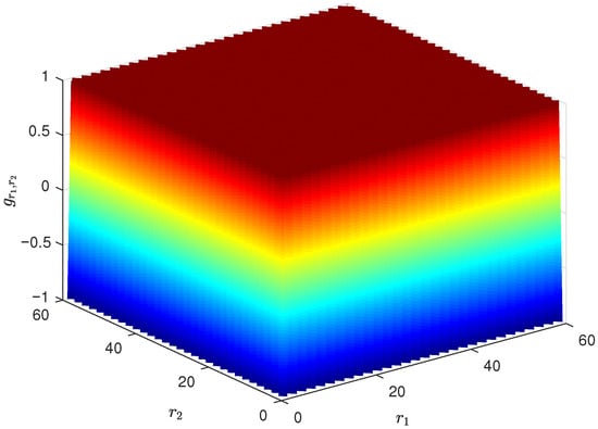
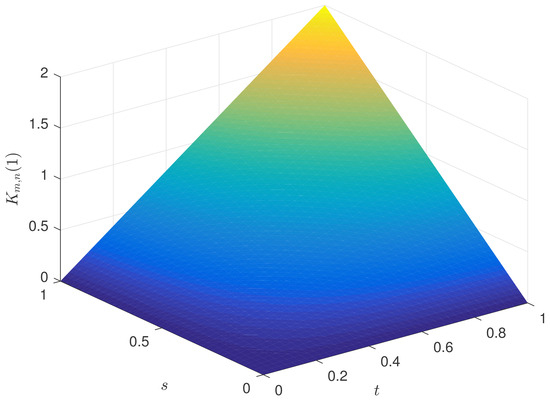
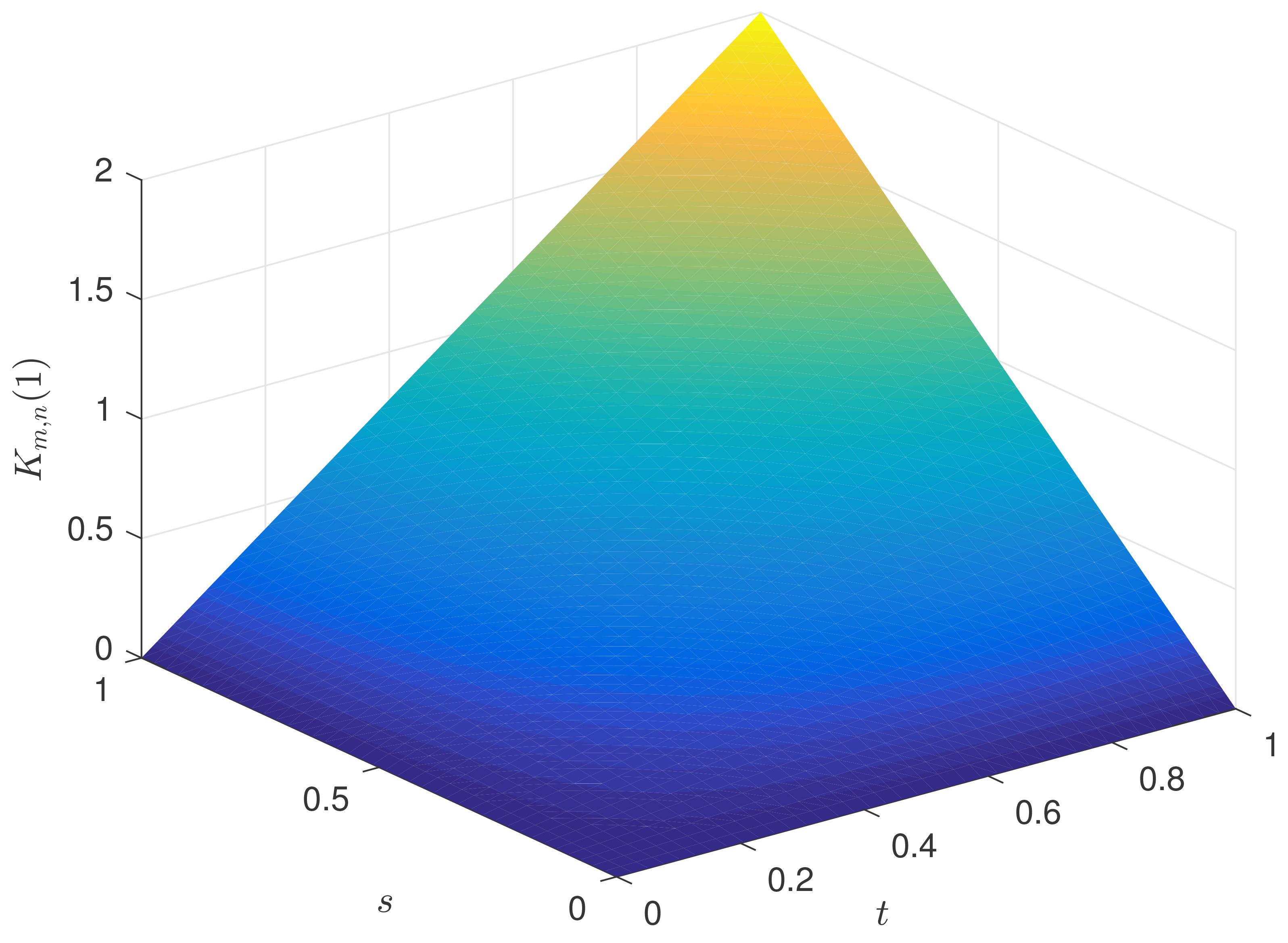
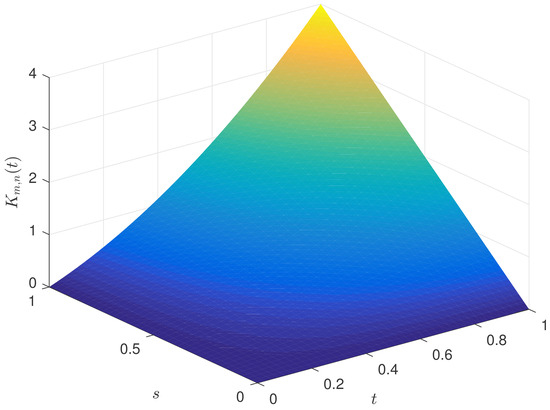
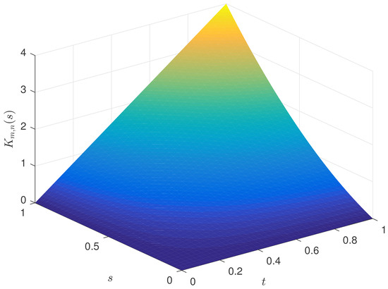
Figure 4 represents the action of the operator on the constant function 1. The resulting surface depends on the product $ts$ together with a bounded oscillatory factor. From a computational perspective, as the indices m and n increase, the influence of the oscillatory term becomes negligible in the statistical sense. Consequently, the surface appears increasingly stable, indicating that the operator preserves constant functions on average and satisfies the first Korovkin test condition.

Figure 5 illustrates the operator applied to the function t. Initially, the surface exhibits mild distortions due to the interaction between the oscillatory factor and the variable t. However, as m and n grow larger, these fluctuations gradually diminish. Computationally, the surface aligns more closely with the shape of the function t, demonstrating that the operator reproduces linear behavior in the t-direction under statistical deferred Cesàro summability.

Figure 6 shows the operator acting on the function s. Its behavior closely mirrors that observed for the function t. Although oscillations are visible for smaller values of m and n, they are averaged out as the parameters increase. As a result, the surface becomes smoother and reflects the linear growth in the s-direction, confirming convergence toward the function s in the statistical sense.

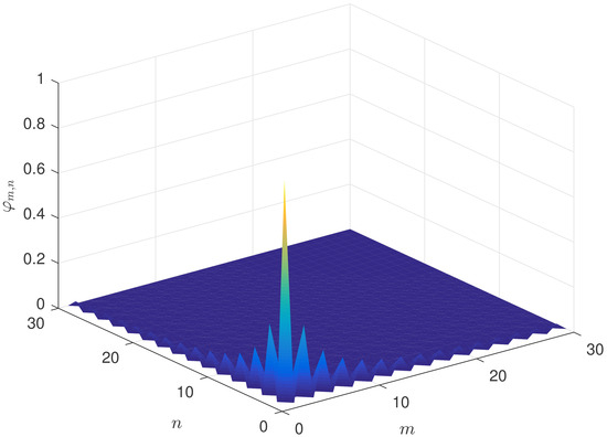
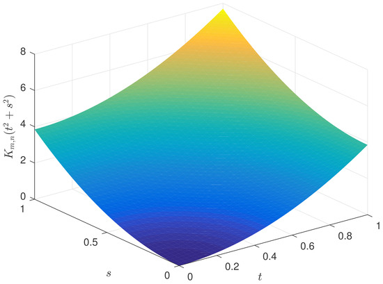
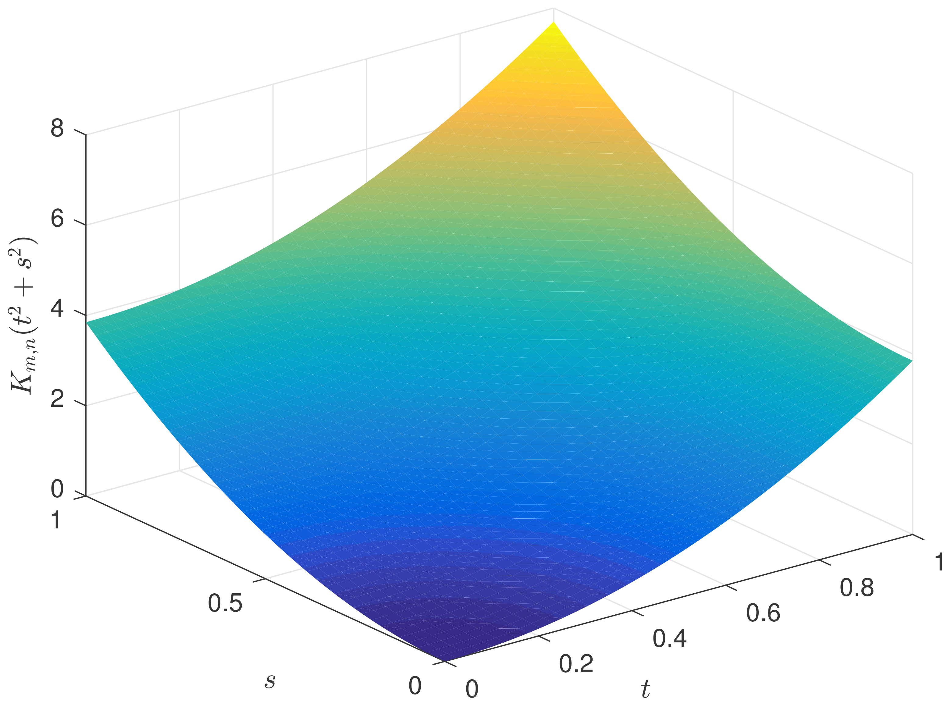
Figure 7 corresponds to the operator applied to the quadratic test function $t^2+s^2$. In this case, the surface initially shows slight deviations due to finite values of m and n. As these parameters tend to infinity, the correction terms diminish and the surface approaches the expected quadratic profile. This computational observation verifies that the operator accurately approximates second-order behavior under statistical deferred Cesàro summability.

Thus, the above numerical illustrations clearly indicate that despite the presence of oscillatory components, the averaged action of the operators converges toward the corresponding test functions. This provides strong computational support for the theoretical conclusion that the operators satisfy all Korovkin-type test conditions under statistical deferred Cesàro summability, ensuring convergence for all continuous functions on the considered time-scale domain.

6. Rate of Deferred Cesàro Summability on Time Scales

In the present section, our objective is to examine the speed of convergence associated with the statistically deferred Cesàro summability of sequences of positive linear operators acting on function spaces defined over product time scales. More precisely, we analyze operators that map the space $\mathcal{C}\left({[a_1,b_1]}_{{\mathbb{T}}_1}\times {[a_2,b_2]}_{{\mathbb{T}}_2}\right)$ onto itself, and we focus on quantifying the corresponding rates of approximation under statistical deferred Cesàro summability.

Definition 6.

Let $\left(a_m\right),$$\left(b_m\right),$$\left(c_n\right)$ and $\left(d_n\right)$ be four sequences of non-negative integers associated with the time-scale ${\mathbb{T}}^2$ such that $a_m<b_m$ and $c_n<d_n$ for all $m,n\in \mathbb{N},$ and

$$\begin{array}{c}\hfill \underset{m\to \infty }{lim}{b}_m=\infty \mathit{and}\underset{n\to \infty }{lim}{d}_n=\infty .\end{array}$$

A double-sequence $\left(g_{m,n}\right)$ of Δ-measurable functions is said to be statistically deferred Cesàro summable to a Δ-measurable function g on ${\mathbb{T}}^2$ with rate $o\left({\gamma }_{m,n}\right)$ if, for each $ϵ>0,$ we have

$$\begin{array}{c}\hfill \underset{m,n\to \infty }{lim}{\displaystyle \frac{{\mu }_{\Delta }\left(E_{\epsilon }\right)}{{\gamma }_{m,n}{\mu }_{\Delta }\left({[a_{m+1},b_m]}_{{\mathbb{T}}_1}\times {[c_{n+1},d_n]}_{{\mathbb{T}}_2}\right)}}=0\end{array}$$

uniformly with respect to $(t,s)\in {\mathbb{T}}^2,$ where

$$\begin{array}{c}\hfill E_{\epsilon }=\left\{(m,n)\in {[a_{m+1},b_m]}_{{\mathbb{T}}_1}\times {[c_{n+1},d_n]}_{{\mathbb{T}}_2}:\left|{\phi }_{m,n}(t,s)-g(t,s)\right|\geqq \epsilon \right\}.\end{array}$$

In this case, we write

$$\begin{array}{c}\hfill {\mathrm{stat}}_{\mathrm{R}\Delta \mathrm{D}}{g}_{m,n}-g=o\left({\gamma }_{m,n}\right)\mathit{on}{\mathbb{T}}^2.\end{array}$$

We now establish Lemma 1 below.

Lemma 1.

Let $\left(a_{m,n}^{\prime }\right)$ and $\left(b_{m,n}^{\prime }\right)$ be two non-increasing double sequences of positive real numbers. Also let $\left(g_{m,n}\right),$$\left(h_{m,n}\right)\in \mathcal{C}\left({[a_1,b_1]}_{{\mathbb{T}}_1}\times {[a_2,b_2]}_{{\mathbb{T}}_2}\right)$ satisfy the conditions given by

$$\begin{array}{c}\hfill {\mathrm{stat}}_{\mathrm{R}\Delta \mathrm{D}}{g}_{m,n}-g=o\left(a_{m,n}^{\prime }\right)\mathit{on}{\mathbb{T}}^2\end{array}$$

and

$$\begin{array}{c}\hfill {\mathrm{stat}}_{\mathrm{R}\Delta \mathrm{D}}{h}_{m,n}-h=o\left(b_{m,n}^{\prime }\right)\mathit{on}{\mathbb{T}}^2.\end{array}$$

Then all the following assertions are true:

(i)

${\mathrm{stat}}_{\mathrm{R}\Delta \mathrm{D}}\left(g_{m,n}+h_{m,n}\right)-(g+h)=o\left(c_{m,n}^{\prime }\right)\mathit{on}{\mathbb{T}}^2;$

(ii)

${\mathrm{stat}}_{\mathrm{R}\Delta \mathrm{D}}\left(g_{m,n}-g\right)\left(h_{m,n}-h\right)=o\left(a_{m,n}^{\prime }{b}_{m,n}^{\prime }\right)\mathit{on}{\mathbb{T}}^2;$

(iii)

${\mathrm{stat}}_{\mathrm{R}\Delta \mathrm{D}}K\left(g_{m,n}-g\right)=o\left(a_{m,n}^{\prime }\right)\mathit{on}{\mathbb{T}}^2$ for any scalar $K;$

(iv)

${\mathrm{stat}}_{\mathrm{R}\Delta \mathrm{D}}{\left(g_{m,n}-g\right)}^{{\displaystyle \frac{1}{2}}}=o\left(a_{m,n}^{\prime }\right)\mathit{on}{\mathbb{T}}^2,$

where

$$\begin{array}{c}\hfill c_{m,n}^{\prime }=max\{a_{m,n}^{\prime },b_{m,n}^{\prime }\}.\end{array}$$

Proof. 

For the assertion (i) of Lemma 1, we consider the following sets for which $\epsilon >0$ and $(t,s)\in {\mathbb{T}}^2$:

$$\begin{array}{cc}\hfill E_{\epsilon }& =\left\{(m,n)\in {[a_{m+1},b_m]}_{{\mathbb{T}}_1}\times {[c_{n+1},d_n]}_{{\mathbb{T}}_2}:\left|({\phi }_{m,n}+{\varphi }_{m,n})-(g+h)\right|\geqq \epsilon \right\},\hfill \end{array}$$

$$\begin{array}{cc}\hfill E_{0,\epsilon }& =\left\{(m,n)\in {[a_{m+1},b_m]}_{{\mathbb{T}}_1}\times {[c_{n+1},d_n]}_{{\mathbb{T}}_2}:\left|{\phi }_{m,n}-g\right|\geqq \epsilon \right\}\hfill \end{array}$$

and

$$\begin{array}{cc}\hfill E_{1,\epsilon }& =\left\{(m,n)\in {[a_{m+1},b_m]}_{{\mathbb{T}}_1}\times {[c_{n+1},d_n]}_{{\mathbb{T}}_2}:\left|{\varphi }_{m,n}-h\right|\geqq \epsilon \right\}.\hfill \end{array}$$

Clearly, we have

$$\begin{array}{c}\hfill E_{\epsilon }\subseteq E_{0,\epsilon }\cup E_{1,\epsilon }.\end{array}$$

Moreover, since

$$\begin{array}{c}\hfill c_{m,n}^{\prime }=max\{a_{m,n}^{\prime },b_{m,n}^{\prime }\},\end{array}$$

(17)

by using assertion (i) of Theorem 6, we obtain

$$\begin{array}{cc}\hfill {\displaystyle \frac{{\mu }_{\Delta }\left(E_{\epsilon }\right)}{c_{m,n}^{\prime }{\mu }_{\Delta }({[a_{m+1},b_m]}_{{\mathbb{T}}_1}\times {[c_{n+1},d_n]}_{{\mathbb{T}}_2})}}& \leqq {\displaystyle \frac{{\mu }_{\Delta }\left(E_{0,\epsilon }\right)}{a_{m,n}^{\prime }{\mu }_{\Delta }({[a_{m+1},b_m]}_{{\mathbb{T}}_1}\times {[c_{n+1},d_n]}_{{\mathbb{T}}_2})}}\hfill \\ \hfill & +{\displaystyle \frac{{\mu }_{\Delta }\left(E_{1,\epsilon }\right)}{b_{m,n}^{\prime }{\mu }_{\Delta }({[a_{m+1},b_m]}_{{\mathbb{T}}_1}\times {[c_{n+1},d_n]}_{{\mathbb{T}}_2})}}.\hfill \end{array}$$

Also, by using assertion (i) of Theorem 6, we obtain

$$\begin{array}{c}\hfill {\displaystyle \frac{{\mu }_{\Delta }\left(E_{\epsilon }\right)}{c_{m,n}^{\prime }{\mu }_{\Delta }({[a_{m+1},b_m]}_{{\mathbb{T}}_1}\times {[c_{n+1},d_n]}_{{\mathbb{T}}_2})}}=0.\end{array}$$

Thus, the assertion (i) of Lemma 1 is proved. We now apply the similar technique for the remaining assertions (ii) to (iv) of Lemma 1 to complete the proof. □

Next, for a function $g:{\mathbb{T}}^2\to \mathbb{R}$, the modulus of continuity of a $\Delta$-measurable function is defined by

$$\begin{array}{cc}\hfill & \omega (g,\delta )=\underset{\begin{array}{c}(t_1,s_1),(t_2,s_2)\in {\mathbb{T}}^2\end{array}}{sup}\{\left|g(t_1,s_1)-g(t_2,s_2)\right|\hfill \\ \hfill & \mathrm{and}\sqrt{{(t_1-t_2)}^2+{(s_1-s_2)}^2}\leqq \delta \left(0<\delta \leqq diam\left({\mathbb{T}}^2\right)\right)\}.\hfill \end{array}$$

We now establish a theorem on the rates of statistically deferred Cesàro summability for double sequences of time-scale positive linear operators with the help of the modulus of continuity defined above.

Theorem 7.

Let $\left(a_m\right),$$\left(b_m\right),$$\left(c_n\right)$ and $\left(d_n\right)$ be four sequences of non-negative integers associated with the time-scale ${\mathbb{T}}^2$. Also let

$$\begin{array}{c}\hfill {\mathfrak{K}}_{m,n}:\mathcal{C}\left({[a_1,b_1]}_{{\mathbb{T}}_1}\times {[a_2,b_2]}_{{\mathbb{T}}_2}\right)⟶\mathcal{C}\left({[a_1,b_1]}_{{\mathbb{T}}_1}\times {[a_2,b_2]}_{{\mathbb{T}}_2}\right)\end{array}$$

be a double sequence of positive linear operators such that

(i)

${\mathrm{stat}}_{\mathrm{R}\Delta \mathrm{D}}{\mathfrak{K}}_{m,n}(1;t,s)-1=o\left(a_{m,n}^{\prime }\right)\mathit{on}{\mathbb{T}}^2;$

(ii)

${\mathrm{stat}}_{\mathrm{R}\Delta \mathrm{D}}\omega \left(g,{\delta }_{m,n}\right)=o\left(b_{m,n}^{\prime }\right)\mathit{on}{\mathbb{T}}^2,$

where

$$\begin{array}{c}\hfill {\delta }_{m,n}(t,s)={\left\{{\mathfrak{K}}_{m,n}\left({\theta }^2;t,s\right)\right\}}^{{\displaystyle \frac{1}{2}}}\mathit{and}\theta (\kappa ,\rho )=\sqrt{{(\kappa -t)}^2+{(\rho -s)}^2}.\end{array}$$

Then, for each $g\in \mathcal{C}\left({[a_1,b_1]}_{{\mathbb{T}}_1}\times {[a_2,b_2]}_{{\mathbb{T}}_2}\right)$, the following assertion holds true:

$$\begin{array}{c}\hfill {\mathrm{stat}}_{\mathrm{R}\Delta \mathrm{D}}{∥{\mathfrak{K}}_{m,n}\left(g\right)-g∥}_{\infty }=o\left(c_{m,n}^{\prime }\right)\mathit{on}{\mathbb{T}}^2,\end{array}$$

(18)

where the double-sequence $\left(c_{m,n}^{\prime }\right)$ is defined analogously to (17).

Proof. 

Suppose that ${\mathbb{T}}^2\subset {\mathbb{R}}^2$ is compact and let

$$\begin{array}{c}\hfill g\in \mathcal{C}\left({[a_1,b_1]}_{{\mathbb{T}}_1}\times {[a_2,b_2]}_{{\mathbb{T}}_2}\right)\left((t,s)\in {\mathbb{T}}^2\right).\end{array}$$

Then we have

$$\begin{array}{cc}\hfill ∥{\mathfrak{K}}_{m,n}(g;t,s)-g(t,s)∥& \leqq \mathcal{Q}∥{\mathfrak{K}}_{m,n}^{*}(1;t,s)-1∥\hfill \\ \hfill & +\left({\mathfrak{K}}_{m,n}^{*}(1;t,s)+\sqrt{{\mathfrak{K}}_{m,n}^{*}(1;t,s)}\right)\omega \left(g,{\delta }_{m,n}\right),\hfill \end{array}$$

where

$$\begin{array}{c}\hfill \mathcal{Q}={\parallel g\parallel }_{\mathcal{C}\left({\mathbb{T}}^2\right)}.\end{array}$$

This yields

$$\begin{array}{cc}\hfill ∥{\mathfrak{K}}_{m,n}\left(g\right)-g∥& \leqq \mathcal{Q}∥{\mathfrak{K}}_{m,n}(1;t,s)-1∥+2\omega \left(g,{\delta }_{m,n}\right)\hfill \\ \hfill & +\omega \left(g,{\delta }_{m,n}\right)\left({\mathfrak{K}}_{m,n}(1;t,s)-1\right)\hfill \\ \hfill & +\omega \left(g,{\delta }_{m,n}\right)\sqrt{{\mathfrak{K}}_{m,n}(1;t,s)-1}.\hfill \end{array}$$

(19)

Finally, using the conditions (i) and (ii) of Theorem 7 together with Lemma 1, inequality (19) implies the desired assertion (18). □

7. Concluding Remarks and Observations

In this concluding section of our investigation, we further observe some concluding remarks of our study presented herein.

Remark 1.

Let ${\left(g_{m,n}\right)}_{m,n\in \mathbb{N}}$ be a double sequence of $\Delta$-measurable functions defined on ${\mathbb{T}}^2,$ as mentioned in Example 2. The double-sequence $\left(g_{m,n}\right)$ is statistically deferred Cesàro summable to 0 so that

$$\begin{array}{c}\hfill {\mathrm{stat}}_{\mathrm{M}\Delta \mathrm{D}}\underset{m,n\to \infty }{lim}{g}_{m,n}=0\mathrm{on}{\mathbb{T}}^2.\end{array}$$

Then we have

$$\begin{array}{c}\hfill {\mathrm{stat}}_{\mathrm{M}\Delta \mathrm{D}}\underset{m,n\to \infty }{lim}{∥{\mathfrak{K}}_{m,n}(g_j;t,s)-g_j(t,s)∥}_{\infty }=0(j=0,1,2,3).\end{array}$$

Thus, by Theorem 6, we immediately get

$$\begin{array}{c}\hfill {\mathrm{stat}}_{\mathrm{M}\Delta \mathrm{D}}\underset{m,n\to \infty }{lim}{∥{\mathfrak{K}}_{m,n}(g;t,s)-g(t,s)∥}_{\infty }=0,\end{array}$$

where

$$\begin{array}{c}\hfill f_0(t,s)=1,f_1(t,s)=t,f_2(t,s)=s\mathrm{and}{f}_3(t,s)=t^2+s^2.\end{array}$$

Since the double-sequence $\left(g_{m,n}\right)$ of time-scale functions is statistically deferred Cesàro summable on ${\mathbb{T}}^2$, while it fails to be either deferred Cesàro statistically convergent or classically convergent on ${\mathbb{T}}^2,$ the Korovkin-type approximation result stated in Theorem 6 remains valid for the operators defined in (16). In contrast, neither the classical nor the statistical convergence of double sequences via deferred Cesàro means holds true for the same operators. This observation demonstrates that Theorem 6 provides a genuine and non-trivial generalization of Theorem 5, as well as the classical Korovkin-type approximation theorem (see [26]).

Remark 2.

Let us suppose that we replace the conditions (i) and (ii) in Theorem 7 with the following condition for a double-sequence $\left\{{\mathfrak{K}}_{m,n}\right\}$ of operators:

$$\begin{array}{c}\hfill {\mathrm{stat}}_{\mathrm{R}\Delta \mathrm{D}}{∥{\mathfrak{K}}_{m,n}(g_j;t,s)-g_j(t,s)∥}_{\mathcal{C}\left({\mathbb{T}}^2\right)}=o\left(a_{m_j,n_j}^{\prime }\right)(j=0,1,2,3).\end{array}$$

(20)

Then, since

$$\begin{array}{cc}\hfill {\mathfrak{K}}_{m,n}({\theta }^2;t,s)& =[{\mathfrak{K}}_{m,n}(t^2+s^2,t,s)-t^2+s^2]-2t[{\mathfrak{K}}_{m,n}(t,t,s)-t]\hfill \\ \hfill & -2s[{\mathfrak{K}}_{m,n}(s,t,s)-s]+t^2[{\mathfrak{K}}_{m,n}(1,t,s)-1],\hfill \end{array}$$

we can write

$$\begin{array}{c}\hfill {\mathfrak{K}}_{m,n}({\theta }^2;t,s)\leqq \mathcal{P}\sum _{j=0}^3{∥{\mathfrak{K}}_{m,n}(g_j;t,s)-g_j(t,s)∥}_{\mathcal{C}\left({\mathbb{T}}^2\right)},\end{array}$$

(21)

where

$$\begin{array}{c}\hfill \mathcal{P}=1+\sum _{j=0}^3{\parallel f_j\parallel }_{\mathcal{C}\left({\mathbb{T}}^2\right)}.\end{array}$$

It now follows from (20), (21) and Lemma 1 that

$$\begin{array}{c}\hfill {\delta }_{m,n}(t,s)=\sqrt{{\mathfrak{K}}_{m,n}({\theta }^2;t,s)}={\mathrm{stat}}_{\mathrm{R}\Delta \mathrm{D}}o\left(d_{m,n}^{\prime }\right),\end{array}$$

where

$$\begin{array}{c}\hfill o\left(d_{k,l}^{\prime }\right)=max\{a_{m_0,n_0}^{\prime },a_{m_1,n_1}^{\prime },a_{m_2,n_2}^{\prime }\}.\end{array}$$

This implies that

$$\begin{array}{c}\hfill {\mathrm{stat}}_{\mathrm{R}\Delta \mathrm{D}}\omega (g,{\delta }_{m,n})=o\left(d_{m,n}^{\prime }\right).\end{array}$$

Now, by using (20) in Theorem 7, we immediately see for $g\in \mathcal{C}\left({\mathbb{T}}^2\right)$ that

$$\begin{array}{c}\hfill {\mathrm{stat}}_{\mathrm{R}\Delta \mathrm{D}}\left|{\mathfrak{K}}_{m,n}(g;t,s)-g(t,s)\right|=o\left(d_{m,n}^{\prime }\right).\end{array}$$

Hence, upon replacing assumptions (i) and (ii) in Theorem 7 with the condition (20) yields the corresponding rate of statistical deferred Cesàro summability for a double sequence of positive linear operators on time scales, as described in Theorem 6.

References

- Zygmund, A. Trigonometric Series, 3rd ed.; Cambridge Mathematical Library, Cambridge University Press: Cambridge, UK, 2002; Volume I and II. [Google Scholar]
- Fast, H. Sur la convergence statistique. Colloq. Math. 1951, 2, 241–244. [Google Scholar] [CrossRef] [Scilit]
- Steinhaus, H. Sur la convergence ordinaire et la convergence asymptotique. Colloq. Math. 1951, 2, 73–74. [Google Scholar]
- Salát, T. On statistically convergent sequences of real numbers. Math. Slovaca 1980, 2, 139–150. [Google Scholar]
- Fridy, J.A. On statistical convergence. Analysis 1985, 5, 301–313. [Google Scholar] [CrossRef] [Scilit]
- Fridy, J.A. Statistical limit points. Proc. Amer. Math. Soc. 1993, 118, 1187–1192. [Google Scholar] [CrossRef]
- Mohiuddine, S.A.; Alotaibi, A.; Mursaleen, M. Statistical summability (C, 1) and a Korovkin type approximation theorem. J. Inequal. Appl. 2012, 2012, 172. [Google Scholar] [CrossRef] [Scilit]
- Srivastava, H.M.; Jena, B.B.; Paikray, S.K.; Misra, U.K. A certain class of weighted statistical convergence and associated Korovkin type approximation theorems involving trigonometric functions. Math. Methods Appl. Sci. 2018, 41, 671–683. [Google Scholar] [CrossRef] [Scilit]
- Srivastava, H.M.; Jena, B.B.; Paikray, S.K. Statistical Riemann and Lebesgue integrable sequence of functions with Korovkin-type approximation theorems. Axioms 2021, 10, 229. [Google Scholar] [CrossRef] [Scilit]
- Srivastava, H.M.; Jena, B.B.; Paikray, S.K. A new class of Korovkin-type theorems on double sequences. Iran. J. Sci. 2025, 49, 1103–1114. [Google Scholar] [CrossRef] [Scilit]
- Jena, B.B.; Paikray, S.K.; Mursaleen, M. Statistical gauge integrable functions and Korovkin-type approximation theorems. Bull. Iran. Math. Soc. 2025, 51, 47. [Google Scholar] [CrossRef] [Scilit]
- Mahapatra, S.C.; Jena, B.B.; Paikray, S.K.; Mursaleen, M. Fuzzy approximation theorems via statistical deferred Nörlund Riemann integrability. Filomat 2025, 39, 9609–9625. [Google Scholar]
- Hilger, S. Ein Maßkettenkalkül mit Anwendung auf Zentrumsmanningfaltigkeiten. Ph.D. Thesis, Universität Würzburg, Würzburg, Germany, 1988. [Google Scholar]
- Hilger, S. Analysis on measure chains: A unified approach to continuous and discrete calculus. Results Math. 1990, 18, 18–56. [Google Scholar] [CrossRef] [Scilit]
- Bohner, M.; Peterson, A. Dynamic Equations on Time Scales: An Introduction with Applications; Birkhaüser Boston, Inc.: Boston, MA, USA, 2001. [Google Scholar]
- Moricz, F. Statistical limits of measurable functions. Analysis 2004, 24, 207–219. [Google Scholar] [CrossRef]
- Guseinov, G.S. Integration on Time Scales. J. Math. Anal. Appl. 2003, 285, 107–127. [Google Scholar] [CrossRef] [Scilit]
- Agarwal, R.P.; Bohner, M. Basic calculus on time scales and some of its applications. Results Math. 1999, 35, 107–127. [Google Scholar] [CrossRef] [Scilit]
- Hilger, S. Laplace and Fourier transform on measure chains. Dyn. Syst. Appl. 1999, 18, 471–488. [Google Scholar]
- Rzezuchowski, T. A note on measures on time scales. Demonstr. Math. 2005, 38, 79–84. [Google Scholar] [CrossRef] [Scilit]
- Seyyidoglu, M.S.; Tan, N.O. A note on statistical convergence on time scale. J. Inequal. Appl. 2012, 2012, 219. [Google Scholar] [CrossRef] [Scilit]
- Turan, C.; Duman, O. Statistical convergence on time scales and its characterization. In Advances in Applied Mathematics and Approximation Theory; Springer: New York, NY, USA, 2013; Volume 41, pp. 57–71. [Google Scholar]
- Agnew, R.P. On deferred Cesàro means. Ann. Math. 1932, 33, 413–421. [Google Scholar] [CrossRef] [Scilit]
- Al-Salam, W.A. Operational representations for the Laguerre and other polynomials. Duke Math. J. 1964, 31, 127–142. [Google Scholar] [CrossRef] [Scilit]
- Viskov, O.V.; Srivastava, H.M. New approaches to certain identities involving differential operators. J. Math. Anal. Appl. 1994, 186, 1–10. [Google Scholar] [CrossRef] [Scilit]
- Korovkin, P.P. Convergence of linear positive operators in the spaces of continuous functions. Doklady Akad. Nauk. SSSR (New Ser.) 1953, 90, 961–964. (In Russian) [Google Scholar]
Disclaimer/Publisher’s Note: The statements, opinions and data contained in all publications are solely those of the individual author(s) and contributor(s) and not of MDPI and/or the editor(s). MDPI and/or the editor(s) disclaim responsibility for any injury to people or property resulting from any ideas, methods, instructions or products referred to in the content. |
© 2026 by the authors. Licensee MDPI, Basel, Switzerland. This article is an open access article distributed under the terms and conditions of the Creative Commons Attribution (CC BY) license.